An efficient GPU-Parallel Coordinate Descent Algorithm for Sparse Precision Matrix Estimation via Scaled Lasso

Abstract

The sparse precision matrix plays an essential role in the Gaussian graphical model since a zero off-diagonal element indicates conditional independence of the corresponding two variables given others. In the Gaussian graphical model, many methods have been proposed and their theoretical properties are given as well. Among these, the sparse precision matrix estimation via scaled lasso (SPMESL) has an attractive feature to which the penalty level is automatically set to achieve the optimal convergence rate under the sparsity and invertibility conditions. Conversely, other methods need to be used in searching for the optimal tuning parameter. Despite such an advantage, the SPMESL has not been widely used due to its expensive computational cost. In this paper, we develop a GPU-parallel coordinate descent (CD) algorithm for the SPMESL and numerically show that the the proposed algorithm is much faster than the least angle regression (LARS) tailored to the SPMESL. Several comprehensive numerical studies are conducted to investigate the scalability of the proposed algorithm and the estimation performance of the SPMESL. The results show that the SPMESL has the lowest false discovery rate for all cases and the best performance in the case where the level of the sparsity of the columns is high.

.

1 Introduction

The covariance matrix and its inverse are of main interest in multivariate analysis to model dependencies between variables. Traditionally, these two parameters have been estimated by the sample covariance matrix and its inverse based on the maximum likelihood (ML) estimation. Although these ML estimators are often asymptotically unbiased and simple to calculate, there are some weaknesses when the number of variables is greater than that of samples. This circumstance is also known as high-dimensional low-sample size (HDLSS) data. For HDLSS data, it is known that the sample covariance matrix becomes inefficient (Yao et al., 2015). In addition, the inverse of the sample covariance matrix is undefined since the sample covariance matrix is singular for HDLSS data. For the covariance matrix, many methods have been proposed under some structural conditions such as bandable structure and sparse structure to improve the estimation efficiency (Bickel and Levina, 2008a, b; Rothman et al., 2009; Wu et al., 2009; Cai et al., 2010; Cai and Liu, 2011a; Cai and Zhou, 2012).

To obtain an estimator of the precision matrix (i.e., inverse covariance matrix) for HDLSS data, various approaches have been developed by adopting the sparsity assumption that there are many zero elements in the matrix. The existing methods can be categorized into four approaches: covariance estimation-induced approach, ML-based approach, regression approach, and constrained $\ell_{1}$-minimization approach. The covariance estimation-induced approach considers an indirect estimation using the inversion of the well-conditioned shrinkage covariance matrix estimators and applies multiple testing procedures to identify nonzero elements of the precision matrix (GeneNet, Schäfer and Strimmer (2005)). The ML-based approach directly estimates the precision matrix by maximizing the penalized likelihood function (Yuan and Lin, 2007; Friedman et al., 2008; Witten et al., 2011; Mazumder et al., 2012). The regression approach considers the linear regression model and uses the fact that the nonzero regression coefficients correspond to the nonzero off-diagonal elements of the precision matrix (Meinshausen and Bühlmann, 2006; Peng et al., 2009; Yuan, 2010; Sun and Zhang, 2013; Ren et al., 2015; Khare et al., 2015; Ali et al., 2017). The constrained $\ell_{1}$-minimization (CLIME) approach (Cai et al., 2011b) obtains the sparse precision matrix by solving the linear programming problem with the constraints on the proximity to the precision matrix where the objective function is the sum of absolute values of the design variables. The adaptive CLIME (Cai et al., 2016) improves the CLIME and attains the optimal rate of convergence.

Among the existing methods, sparse precision matrix estimation via the scaled Lasso (SPMESL) proposed by Sun and Zhang (2013) is a tuning-free procedure. Conversely, other existing methods require searching the optimal tuning parameter, GeneNet (Schäfer and Strimmer, 2005) and the neighborhood selection (Meinshausen and Bühlmann, 2006) require choosing the level of the false discovery rate; other penalized methods require choosing the optimal penalty level. In addition, SPMESL supports the consistency of the precision matrix estimation under the sparsity and invertibility conditions that are weaker than the irrepresentable condition (van de Geer and Bühlmann, 2009; Sun and Zhang, 2013). However, it has not been widely used for the sparse precision matrix estimation due to the inefficiency of the implemented algorithm of the SPMESL using the least angle regression (LARS) algorithm (Efron et al., 2004). Even though the LARS algorithm efficiently provides a whole solution path of the Lasso problem (Tibshirani, 1996), its computational cost is expensive and the SPMESL needs to solve $p$ independent Lasso problems as the subproblems of the SPMESL. Thus, the scalability of the SPMESL is still challenging.

In this paper, we found the possibility to improve the computational efficiency of the SPMESL with the empirical observation that the SPMESL does not need a whole solution path of the Lasso problem based on the tuning-free characteristic of the SPMESL (see details in Section 3). Motivated by this empirical observation, we propose a more efficient algorithm based on the coordinate descent (CD) algorithm and the warm start strategy for the scaled Lasso and the SPMESL as applied to the standard lasso problem in Wu and Lange (2008). Moreover, we develop the row-wise updating parallel CD algorithm using graphics processing units (GPUs) adequate for the SPMESL. To efficiently implement the proposed parallel CD algorithm, we consider the active response matrix that consists of columns of active response variables that corresponds to the error variance estimate not converged at the current iteration. We will show the efficiency of the proposed algorithms using comprehensive numerical studies. In this paper, we also provide the numerical comparisons of the estimation performance of the SPMESL with three different penalty levels, which are theoretically suggested in previous literature (Sun and Zhang, 2012, 2013) but there is no comparison result of them in terms of the estimation performance.

The remainder of the paper is organized as follows. Section 2 introduces the SPMESL and its original algorithm. We explain the proposed CD algorithm and GPU-parallel CD algorithm in Section 3. Section 4 provides a comprehensive numerical study, including the comparisons of computation times and estimation performances with other existing methods. We provide a summary of the paper and discussion in Section 5.

2 Sparse Precision Matrix Estimation via Scaled Lasso

In this section, we briefly introduce the scaled Lasso, the SPMESL, and their algorithms.

2.1 Scaled Lasso

The scaled Lasso proposed by Sun and Zhang (2012) is a variant of a penalized regression model with the Lasso penalty. To be specific, let ${\bf y}\in\mathbb{R}^{n}$, ${\bf X}\in\mathbb{R}^{n\times p}$, $\boldsymbol{\beta}\in\mathbb{R}^{p}$, and $\sigma>0$. Consider a linear regression model ${\bf y}={\bf X}\boldsymbol{\beta}+\epsilon$, where $\epsilon\sim N(0,\sigma^{2}{\bf I}_{n})$ and ${\bf I}_{n}$ is the $n$-dimensional identity matrix. The scaled Lasso considers the minimization of the following objective function $L_{\lambda_{0}}(\boldsymbol{\beta},\sigma)$:

$$L_{\lambda_{0}}(\boldsymbol{\beta},\sigma)=\frac{\|{\bf y}-{\bf X}\boldsymbol{\beta}\|_{2}^{2}}{2n\sigma}+\frac{\sigma}{2}+\lambda_{0}\|\boldsymbol{\beta}\|_{1},$$ (1)

where $\lambda_{0}$ is a given tuning parameter and $\|{\bf x}\|_{1}=\sum_{j=1}^{p}|x_{j}|$ for ${\bf x}\in\mathbb{R}^{p}$. Thus, the scaled Lasso simultaneously obtains the estimate $\hat{\boldsymbol{\beta}}$ of the regression coefficient $\boldsymbol{\beta}$ and the estimate $\hat{\sigma}$ of the error standard deviation $\sigma$. It is proved that the objective function $L_{\lambda_{0}}$ is jointly convex in $(\boldsymbol{\beta},\sigma)$ and is strictly convex for $\sigma$ in Sun and Zhang (2012). From the convexity of the objective function, the solution $(\hat{\boldsymbol{\beta}},\hat{\sigma})$ of the scaled Lasso problem can be obtained by the block CD algorithm as follows:

• (Step 1) With a fixed $\hat{\sigma}$, consider the minimization of $\hat{\sigma}L_{\lambda_{0}}(\boldsymbol{\beta},\hat{\sigma})$:

  $$\hat{\sigma}L_{\lambda_{0}}(\boldsymbol{\beta},\hat{\sigma})=\frac{\|{\bf y}-{\bf X}\boldsymbol{\beta}\|_{2}^{2}}{2n}+\hat{\sigma}\lambda_{0}\|\boldsymbol{\beta}\|_{1}+\frac{\hat{\sigma}^{2}}{2}.$$

  The minimizer $\hat{\boldsymbol{\beta}}$ of $\hat{\sigma}L_{\lambda_{0}}(\boldsymbol{\beta},\hat{\sigma})$ can be obtained by solving the following standard lasso problem with $\lambda=\hat{\sigma}\lambda_{0}$:

  $$\min_{\boldsymbol{\beta}}\frac{\|{\bf y}-{\bf X}\boldsymbol{\beta}\|_{2}^{2}}{2n}+\lambda\|\boldsymbol{\beta}\|_{1}.$$ (2)

• (Step 2) With a fixed $\hat{\boldsymbol{\beta}}$, the minimizer $\hat{\sigma}$ of $L_{\lambda_{0}}(\hat{\boldsymbol{\beta}},\sigma)$ is easily obtained by

  $$\hat{\sigma}=\frac{\|{\bf y}-{\bf X}\hat{\boldsymbol{\beta}}\|_{2}}{\sqrt{n}}.$$

• (Step 3) Repeat Steps 1 and 2 until convergence occurs.

In the original paper of the scaled Lasso, the standard lasso problem is solved by the LARS algorithm (Efron et al., 2004), which provides a whole solution path of the standard Lasso problem. During the block CD algorithm, the minimizer $\hat{\boldsymbol{\beta}}(\hat{\sigma}^{(r)})$ of $\hat{\sigma}^{(r)}L_{\lambda_{0}}(\boldsymbol{\beta},\hat{\sigma}^{(r)})$ in Step 1 at the $r$-th iteration is obtained from the solution path of the standard Lasso problem with $\lambda=\hat{\sigma}^{(r)}\lambda_{0}$.

In addition to the joint estimation of $\boldsymbol{\beta}$ and $\sigma$, the scaled Lasso has attractive features as described in Sun and Zhang (2012). First, the scaled Lasso guarantees the consistency of $\hat{\boldsymbol{\beta}}$ and $\hat{\sigma}$ under two conditions: the penalty level condition $\lambda_{0}>A\sqrt{2n^{-1}\log p}$ for $A>1$ and the compatibility condition, which implies the oracle inequalities for the prediction and estimation (van de Geer and Bühlmann, 2009). Second, the scaled Lasso estimates are scale-equivariant in ${\bf y}$ in the sense that $\hat{\boldsymbol{\beta}}({\bf X},\alpha{\bf y})=\alpha\hat{\boldsymbol{\beta}}({\bf X},{\bf y})$ and $\hat{\sigma}({\bf X},\alpha{\bf y})=|\alpha|\hat{\sigma}({\bf X},{\bf y})$. Finally, the authors suggest using the universal penalty level $\lambda_{0}^{U}=\sqrt{2n^{-1}\log p}$ for $\lambda_{0}$ based on their numerical and real-data examples. We can consider the scaled Lasso with the universal penalty level as a tuning-free procedure. Note that the universal penalty level does not satisfy the theoretical requirement $\lambda_{0}>A\sqrt{2n^{-1}\log p}$ for the consistency of $\hat{\sigma}$. The authors of the scaled Lasso provide several conditions that can weaken the required condition for $\lambda_{0}$, in order to justify using a penalty level smaller than $A\sqrt{2n^{-1}\log p}$ for $A>1$ (Sun and Zhang, 2012).

2.2 Sparse precision matrix estimation via scaled Lasso

Let $\boldsymbol{\Sigma}=(\sigma_{jk})_{1\leq j,k\leq p}$ and $\boldsymbol{\Omega}=\boldsymbol{\Sigma}^{-1}=(\omega_{jk})_{1\leq j,k\leq p}$ be a covariance matrix and a corresponding precision matrix, respectively. Suppose that ${\bf x}^{(i)}=(X_{i1},\ldots,X_{ip})$ for $i=1,2,\ldots,n$ are independently drawn from the multivariate normal distribution with mean ${\bf 0}$ and covariance matrix $\boldsymbol{\Sigma}$. Let ${\bf X}\in\mathbb{R}^{n\times p}$ be a data matrix and ${\bf x}_{k}=(X_{1k},\ldots,X_{nk})^{T}$ be the $k$th column of ${\bf X}$. Consider following linear regression models for $k=1,\ldots,p$:

$$X_{ik}=\sum_{l\neq k}\beta_{lk}X_{il}+\epsilon_{ik},~{}$$ (3)

where $\epsilon_{ik}$s are independent and identically distributed random variables drawn from the normal distribution with mean 0 and variance $\sigma_{k}^{2}$. As applied in the regression approach for the sparse precision matrix estimation, the elements of the precision matrix can be represented into the regression coefficient and the error variance by using the following relationships:

$$\omega_{jk}=-\frac{\beta_{jk}}{\sigma_{k}^{2}},~{}\omega_{kk}=\frac{1}{\sigma_{k}^{2}}~{}\mbox{ for }1\leq j\neq k\leq p.$$ (4)

As the scaled Lasso simultaneously estimates the regression coefficients $(\beta_{jk})$ and the error standard deviation $\sigma_{k}$ as described in Section 2.1, we can use the scaled Lasso to estimate the precision matrix. Thus, the SPMESL considers solving the scaled Lasso problems column-wise and defines the SPMESL estimator that combines the estimates from the $p$ scaled Lasso problems.

To be specific, let $\textbf{B}=(b_{jk})_{1\leq j,k\leq p}$ be a matrix of the regression coefficients such that $b_{jk}=\beta_{jk}$ for $j\neq k$ and $b_{jj}=-1$ for $j=1,\ldots,p$. Denote ${\bf b}^{(j)}=(b_{j1},\ldots,b_{jp})$ and ${\bf b}_{k}=(b_{1k},\ldots,b_{pk})^{T}$ as the $j$th row and the $k$th column of a matrix ${\bf B}$, respectively. We further let ${\bf S}=(s_{jk})$ be the sample covariance matrix. Subsequently, the precision matrix can be represented with ${\bf B}$ and ${\bf D}={\rm diag}(\sigma_{1}^{-2},\ldots,\sigma_{p}^{-2})$ as follows:

$$\boldsymbol{\Omega}=-{\bf B}{\bf D}=(-\sigma_{1}^{-2}{\bf b}_{1},\ldots,-\sigma_{p}^{-2}{\bf b}_{p}).$$

To obtain the estimate of $\boldsymbol{\Omega}$, the SPMESL solves the following $p$ independent scaled Lasso problems first: for $k=1,\ldots,p$,

$$(\hat{\bf b}_{k},\hat{\sigma}_{k})=\operatornamewithlimits{argmin}_{\boldsymbol{\beta}_{k}\in\mathbb{R}^{p}:\beta_{kk}=-1,\sigma_{k}>0}~{}\frac{\|{\bf X}_{k}-\sum_{j\neq k}\beta_{jk}{\bf X}_{j}\|_{2}^{2}}{2n\sigma_{k}}+\frac{\sigma_{k}}{2}+\lambda_{0}\sum_{j\neq k}|\beta_{jk}|.$$ (5)

Note that the SPMESL in Sun and Zhang (2013) originally considers $\lambda_{0}\sum_{j\neq k}\sqrt{s_{jj}}|\beta_{jk}|$ instead of $\lambda_{0}\sum_{j\neq k}|\beta_{jk}|$ to penalize the coefficients on the same scale. In this paper, we assume that the columns of the data matrix ${\bf X}$ are centered and scaled to ${\bf X}_{k}^{T}{\bf X}_{k}=n$ for $k=1,\ldots,p$. Thus, $s_{jj}=1$ for $j=1,\ldots,p$. This assumption does not affect the estimation performance of the precision matrix as the scaled Lasso has the scale-equivariant property in the response variable as explained in the previous section. We can easily recover the estimate $\hat{\boldsymbol{\Omega}}^{o}=(\hat{\omega}_{jk}^{o})_{1\leq j,k\leq p}$ from the data in the original scale by the following Proposition 1:

Proposition 1

Let ${\bf X}\in\mathbb{R}^{n\times p}$ and $\tilde{{\bf X}}={\bf X}{\bf C}$ be a data matrix and the scaled data matrix with ${\bf C}={\rm diag}(s_{11}^{-1/2},\ldots,s_{pp}^{-1/2})$, where $s_{jj}>0$ for $j=1,\ldots,p$. Denote $\hat{\boldsymbol{\Omega}}^{o}$ as the estimate of the precision matrix by applying the scaled Lasso in (5) with the penalty term $\lambda_{0}\sum_{j\neq k}\sqrt{s_{jj}}|\beta_{jk}|$ column by column with ${\bf X}$. Similarly, denote $\hat{\boldsymbol{\Omega}}^{C}=(\hat{\omega}_{jk}^{C})_{1\leq j,k\leq p}$ as the estimate by the scaled Lasso in (5) with $\tilde{{\bf X}}$. Then, $\hat{\boldsymbol{\Omega}}^{o}={\bf C}\hat{\boldsymbol{\Omega}}^{C}{\bf C}$.

Proof

By the definition of $\tilde{{\bf X}}$, the $k$th column of $\tilde{{\bf X}}$ is $\tilde{{\bf X}}_{k}={\bf X}_{k}/\sqrt{s_{kk}}$. Let $\hat{\bf B}^{C}=(\hat{b}_{jk}^{C})_{1\leq j,k\leq p}$ and $(\hat{\sigma}_{k,C})_{1\leq k\leq p}$ be the solutions of the $p$ scaled Lasso problem in (5) with $\tilde{{\bf X}}$. We further let $\hat{\bf B}^{o}=(\hat{b}_{jk}^{o})_{1\leq j,k\leq p}$ and $(\hat{\sigma}_{k,o})_{1\leq k\leq p}$ be the solutions of the following scaled Lasso problems: for $k=1,\ldots,p$,

$$(\hat{\bf b}_{k}^{o},\hat{\sigma}_{k,o})=\operatornamewithlimits{argmin}_{\boldsymbol{\beta}_{k}\in\mathbb{R}^{p}:\beta_{kk}=-1,\sigma_{k}>0}~{}\frac{\|{\bf X}_{k}-\sum_{j\neq k}\beta_{jk}{\bf X}_{j}\|_{2}^{2}}{2n\sigma_{k}}+\frac{\sigma_{k}}{2}+\lambda_{0}\sum_{j\neq k}\sqrt{s_{jj}}|\beta_{jk}|.$$ (6)

By substituting $\tilde{{\bf X}}$ with ${\bf X}{\bf C}$ in (5) and the reparameterization with $\tilde{\beta}_{jk}=\beta_{jk}/\sqrt{s_{jj}}$ for $j\neq k$, the $k$th scaled Lasso problem becomes

$$(\hat{\bf b}_{k}^{C},\hat{\sigma}_{k,C})=\operatornamewithlimits{argmin}_{\tilde{\boldsymbol{\beta}}_{k}\in\mathbb{R}^{p}:\tilde{\beta}_{kk}=-1,\sigma_{k}>0}~{}\frac{\|{\bf X}_{k}/\sqrt{s_{kk}}-\sum_{j\neq k}\tilde{\beta}_{jk}{\bf X}_{j}\|_{2}^{2}}{2n\sigma_{k}}+\frac{\sigma_{k}}{2}+\lambda_{0}\sum_{j\neq k}\sqrt{s_{jj}}|\tilde{\beta}_{jk}|.$$ (7)

From the forms of the problems (6) and (7), the relationship $\hat{\bf b}^{o}_{k}=\sqrt{s_{kk}}\hat{\bf b}^{C}_{k}$ and $\hat{\sigma}_{k,o}=\sqrt{s_{kk}}\hat{\sigma}_{k,C}$ hold by the scale equivariant property of the scaled Lasso. In addition, by the reparameterization, $\hat{b}^{o}_{jk}=\sqrt{s_{kk}/s_{jj}}\hat{b}^{C}_{jk}$ for $1\leq j,k\leq p$. Combining the above relationships, the $(j,k)$th element $\hat{\omega}_{jk}^{o}$ of the precision matrix estimate $\hat{\boldsymbol{\Omega}}^{o}$ is represented as

$$\hat{\omega}_{jk}^{o}=-\hat{b}_{jk}^{o}\hat{\sigma}_{k,o}^{-2}=-(s_{jj}s_{kk})^{-1/2}\hat{b}_{jk}^{C}\hat{\sigma}_{k,C}^{-2}=(s_{jj}s_{kk})^{-1/2}\hat{\omega}_{jk}^{C}.$$

Hence, $\hat{\boldsymbol{\Omega}}^{o}={\bf C}\hat{\boldsymbol{\Omega}}^{C}{\bf C}$.

Note that the result $\hat{\boldsymbol{\Omega}}^{o}={\bf C}\hat{\boldsymbol{\Omega}}^{C}{\bf C}$ in Proposition 1 is consistent with the property of $({\rm Var}({\bf A}{\bf z}))^{-1}={\bf A}^{-T}{\rm Var}({\bf z})^{-1}{\bf A}^{-1}$ for a $p$-dimensional random vector ${\bf z}$ and a nonsingular matrix ${\bf A}\in\mathbb{R}^{p\times p}$.

After solving $p$ independent scaled Lasso problems, the estimate $\hat{\boldsymbol{\Omega}}_{1}=-\hat{\bf B}\hat{\bf D}=(\hat{\omega}_{jk,1})_{1\leq j,k\leq p}$ of the precision matrix is obtained. However, the estimate $\hat{\boldsymbol{\Omega}}_{1}$ is not symmetric in general. To find the symmetric estimate of the precision matrix using the current estimate $\hat{\boldsymbol{\Omega}}_{1}$, the SPMESL considers solving the following linear programming problem as in Yuan (2010):

$$\hat{\boldsymbol{\Omega}}=\operatornamewithlimits{argmin}_{{\bf M}:{\bf M}^{T}={\bf M}}\|{\bf M}-\hat{\boldsymbol{\Omega}}_{1}\|_{1}.$$ (8)

Remark that the authors of the SPMESL consider the above linear programming problem for the symmetrization step in Sun and Zhang (2013), but they applied the following symmetrization step in the implemented R package scalreg:

$$\hat{\omega}_{jk}=\hat{\omega}_{kj}=\hat{\omega}_{jk,1}I(|\hat{\omega}_{jk,1}|\leq|\hat{\omega}_{kj,1}|)+\hat{\omega}_{kj,1}I(|\hat{\omega}_{jk,1}|>|\hat{\omega}_{kj,1}|),$$ (9)

which is applied in the CLIME and the theoretical properties are developed on this symmetrization (Cai et al., 2011b). In addition, for the high-dimensional data, the symmetrization applied in the CLIME is favorable as its computational cost is cheap and it is easily parallelizable. For these reasons, we apply the symmetrization step (9) in the proposed algorithm.

As stated in the previous section, the scaled Lasso guarantees the consistency of the regression coefficients and the error variance under the compatibility condition. Thus, the SPMESL also guarantees column-wise consistency of $\hat{\boldsymbol{\Omega}}_{1}$ under the compatibility conditions, which is independently defined in each column of $\hat{\boldsymbol{\Omega}}_{1}$, as the SPMESL applies the scaled Lasso column wise. To derive the overall consistency of $\hat{\boldsymbol{\Omega}}$, the authors of the SPMESL considers the capped $\ell_{1}$ sparsity and the invertibility conditions as follows.

1. Capped $\ell_{1}$ sparsity condition: For a certain $\epsilon_{0}$, $\lambda_{0}^{*}$ not depending on $j$ and an index set $T_{j}\subset\{1,2,\ldots,p\}\setminus\{j\}$, the capped $\ell_{1}$ sparsity of the $j$th column with $t_{j}>0$ is defined as

   $$|T_{j}|+\sum_{k\neq j,k\notin S_{j}}\frac{|\omega_{kj}|\sqrt{\sigma_{kk}}}{(1-\epsilon_{0})\sqrt{\omega_{jj}}\lambda_{0}^{*}}\leq a_{j}.$$

2. Invertibility condition: Let ${\bf W}={\rm diag}(\sigma_{11},\ldots,\sigma_{pp})$ and ${\bf R}={\bf W}^{-1/2}\boldsymbol{\Sigma}{\bf W}^{-1/2}$. Further, let $T_{j}\subseteq Q_{j}\subseteq\{1,2,\ldots,p\}\setminus\{j\}$. The invertibility condition is defined as

   $$\inf_{j}\left\{\frac{{\bf u}^{T}{\bf R}_{-j,-j}{\bf u}}{\|{\bf u}_{Q_{j}}\|_{2}^{2}}~{}:~{}{\bf u}\in\mathbb{R}^{p},{\bf u}_{Q_{j}}\neq 0,1\leq j\leq p\right\}\geq c_{*}$$

   with a fixed constant $c_{*}>0$. Note that the invertibility condition holds if the spectral norm of ${\bf R}^{-1}={\bf D}^{1/2}\boldsymbol{\Omega}{\bf D}^{1/2}$ is bounded (i.e., $\|{\bf R}^{-1}\|_{2}\leq c_{*}^{-1}$).

With some modifications on the capped $\ell_{1}$ sparsity and the invertibility conditions, the authors of the SPMESL derive several conditions on $\lambda_{0}^{*}$ that guarantees the estimation consistency of the precision matrix under the spectral norm. Among them, for practical usage, we consider two conditions on a penalty level $\lambda_{0}\geq\lambda_{0}^{*}$ as follows:

• Union bound for $p$ applications of the scaled Lasso (Theorem 2 in Sun and Zhang (2013)):

  $$\lambda_{0}=A\sqrt{4n^{-1}\log p}\mbox{ for }A>1.$$ (10)

• Probabilistic error bound (Theorem 13 in Sun and Zhang (2013)):

  $$\lambda_{0}=AL_{n}(k/p)\mbox{ for }1<A\leq\sqrt{2},$$ (11)

  where $k$ is a real solution of $k=L_{1}^{4}(k/p)+2L_{1}^{2}(k/p)$, $L_{n}(t)=n^{-1/2}\Phi^{-1}(1-t)$, and $\Phi^{-1}(t)$ is the standard normal quantile function.

Note that a real solution of the equation $k-L_{1}^{4}(k/p)+2L_{1}^{2}(k/p)=0$ can easily be found by applying the bisection method. For instance, we demonstrate two real solutions for $p=100,1000$ in Figure 1 with the values of $k-L_{1}^{4}(k/p)+2L_{1}^{2}(k/p)$. For $p=1000$ and $n=100$, $\lambda_{ub}=\sqrt{4n^{-1}\log p}\approx 0.5257$ and $\lambda_{pb}=\sqrt{2}L_{n}(k/p)\approx 0.2810$ with $k=23.4748$ while $\lambda_{univ}=\sqrt{2n^{-1}\log(p-1)}\approx 0.3717$, where $\lambda_{ub}$ is the penalty level derived by the union bound, $\lambda_{pb}$ is the penalty level derived by the probabilistic error bound, and $\lambda_{univ}$ is the universal penalty level used in the scaled lasso. In the paper of Sun and Zhang (2013), the penalty level derived by the probabilistic error bound is suggested for the SPMESL. However, there are no comparison results for the three penalty levels $\lambda_{univ}$, $\lambda_{ub}$, and $\lambda_{pb}$. We conduct a comparison of performances for identifying the nonzero elements of $\boldsymbol{\Omega}$ by the three penalty levels above in Section 4 to provide a guideline for the penalty level $\lambda_{0}$.

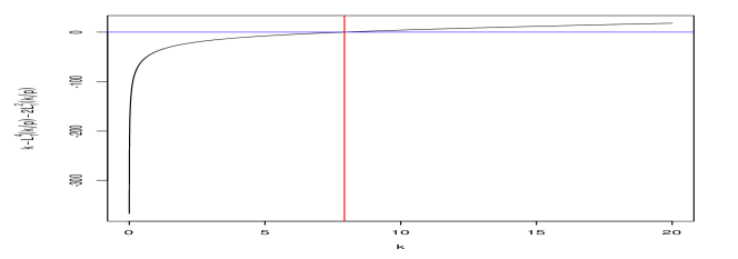
(1) $p=100$

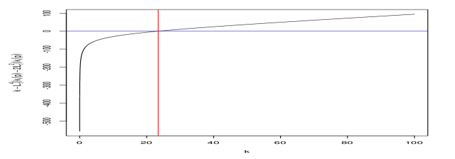
(2) $p=1000$

Figure 1: Plots of $k-L_{1}^{4}(k/p)+2L_{1}^{2}(k/p)$ for $p=100,1000$. Vertical red lines denote the solutions of $k-L_{1}^{4}(k/p)+2L_{1}^{2}(k/p)=0$ obtained by the bisection method.

3 Efficient Coordinate Descent Algorithm for SPMESL and its GPU-parallelization

The original algorithm for the scaled Lasso and the SPMESL adopt the LARS algorithm, which provides the whole solution path of the Lasso regression problem, and its implemented R package scalreg is available in the Comprehensive R Archive Network (CRAN) repository. As mentioned in the Introduction, we empirically observed that the block CD algorithms for the scaled Lasso and the SPMESL do not need a whole solution path of the standard Lasso problem in their sub-problems, where the sub-problem denotes the minimization problem in Step 1 of the scaled Lasso problem. To describe our empirical observation, we consider an example with a linear regression model $y_{i}={\bf x}_{i}^{T}\boldsymbol{\beta}+\epsilon_{i}$ and $\epsilon_{i}\sim N(0,\sigma^{2})$ for $i=1,2,\ldots,250$, where the true parameter $\boldsymbol{\beta}=(\boldsymbol{\beta}_{2}^{T},\boldsymbol{\beta}_{-1}^{T},\boldsymbol{\beta}_{0}^{T})^{T}\in\mathbb{R}^{500}$, $\boldsymbol{\beta}_{2}=(2,\ldots,2)^{T}\in\mathbb{R}^{5}$, $\boldsymbol{\beta}_{-1}=(-1,\ldots,-1)^{T}\in\mathbb{R}^{5}$, $\boldsymbol{\beta}_{0}=(0,\ldots,0)^{T}\in\mathbb{R}^{490}$, and $\sigma=3,5$. We set the initial value of $(\boldsymbol{\beta},\sigma)$ as $({\bf 0}_{500\times 1},1)$. As shown in Figure 2, the numbers of iterations for the convergence of $\hat{\sigma}$ are less than 10 when the true parameter $\sigma=3,5$ and $\lambda_{0}=\sqrt{2n^{-1}\log p}$. This implies that we do not need to obtain the whole solution paths of $p$ lasso problems with respect to all $\lambda$ values.

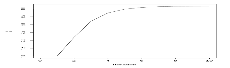
(1) $p=500,n=250,\sigma=3$

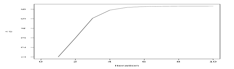
(2) $p=500,n=250,\sigma=5$

Figure 2: Plots of the estimates of $\hat{\sigma}$ for $\sigma=3,5$ along with the number of iterations.

Thus, the calculation of the whole solution path by the LARS algorithm is inefficient for the scaled Lasso and the SPMESL. In addition, the scaled Lasso and the SPMESL iteratively solve the lasso problem with the penalty $\lambda_{r}=\hat{\sigma}^{(r)}\lambda_{0}$ in their inner iteration, where $\lambda_{r}$ denotes the penalty level at the $r$th iteration. As $\hat{\sigma}^{(r)}$ converges to the minimizer of (1), the difference between $\lambda_{r}$ and $\lambda_{r-1}$ decreases as the iteration proceeds. This denotes that the Lasso estimate in the current iteration is not far from that in the next iteration. From this observation, the warm start strategy, which denotes that the solution in the previous iteration is used as an initial value of the next iteration, is favorable and can efficiently accelerate the algorithm for the Lasso regression problem in the inner iteration.

To fully utilize the warm start strategy, we consider the coordinate descent (CD) algorithm for the Lasso regression problem in the inner iteration. This is because it is known that the CD algorithm with the warm start strategy is efficient for the Lasso regression problem and has an advantage for memory consumption (Wu and Lange, 2008). In addition, the SPMESL needs solving $p$ independent scaled Lasso problems to obtain the estimate of the precision matrix. We develop the GPU-parallel CD algorithm for the SPMESL, which updates $p$ coordinates simultaneously with GPUs. In the following subsections, we introduce the CD algorithm for the subproblem of the scaled Lasso and GPU-parallel CD algorithm for the SPMESL in detail.

3.1 CD Algorithm for subproblem of the scaled Lasso

In this subsection, we focus on the following subproblem of the scaled Lasso with a given $\lambda_{0}$:

$$\hat{\boldsymbol{\beta}}^{(r)}=\operatornamewithlimits{argmin}_{\boldsymbol{\beta}}\frac{1}{2n}\|{\bf y}-{\bf X}\boldsymbol{\beta}\|_{2}^{2}+\lambda^{(r-1)}\|\boldsymbol{\beta}\|_{1},$$ (12)

where ${\bf y}\in\mathbb{R}^{n}$ is a response vector, ${\bf X}\in\mathbb{R}^{n\times p}$ is a design matrix, $\lambda^{(r-1)}=\hat{\sigma}^{(r-1)}\lambda_{0}$, and $\hat{\sigma}^{(r-1)}=\|{\bf y}-{\bf X}\hat{\beta}^{(r-1)}\|_{2}/\sqrt{n}$ is the iterative solution for $\sigma$ at the $(r-1)$th iteration. For the notational simplicity, we use $\hat{\boldsymbol{\beta}}$ to denote the $r$th iterative solution $\hat{\boldsymbol{\beta}}^{(r)}$, and $\hat{\boldsymbol{\beta}}^{[cur]}$ and $\hat{\boldsymbol{\beta}}^{[next]}$ denote the current and the next iterative solution in the CD algorithm, respectively. To apply the warm start strategy, we set the initial value $\hat{\boldsymbol{\beta}}^{[cur]}$ for $\hat{\boldsymbol{\beta}}$ to $\hat{\boldsymbol{\beta}}^{(r-1)}$. In this paper, we consider the cyclic CD algorithm with an ascending order (i.e., coordinate-wise update from the smallest index to the largest index). Subsequently, for $j=1,\ldots,p$, the CD algorithm updates $\hat{\beta}_{j}^{[next]}$ by following equations:

$${\bf e}_{j}={\bf y}-\sum_{l<j}{\bf X}_{l}\hat{{\beta}}_{l}^{[next]}-\sum_{l>j}{\bf X}_{l}\hat{{\beta}}_{l}^{[cur]},\quad a_{j}={\bf x}_{j}^{T}{\bf e}_{j}/n+\hat{\beta}_{j}^{[cur]},\quad\hat{\beta}_{j}^{[next]}=\mbox{Soft}_{\lambda}(a_{j}),$$

where $\mbox{Soft}_{\lambda}(a_{j})=\mbox{sign}(a_{j})(|a_{j}|-\lambda)_{+}$ is the soft-thresholding operator and $(x)_{+}=\max(x,0)$. The CD algorithm repeats the cyclic updates until the convergence occurs, where the common convergence criterion is the $L_{\infty}$-norm of the difference between $\hat{\boldsymbol{\beta}}^{[cur]}$ and $\hat{\boldsymbol{\beta}}^{[next]}$ (i.e., $\|\hat{\boldsymbol{\beta}}^{[next]}-\hat{\boldsymbol{\beta}}^{[cur]}\|_{\infty}$). The whole CD algorithm with warm start strategy for the scaled Lasso is summarized in Algorithm 1.

Algorithm 1 CD algorithm with warm start strategy for the scaled Lasso

1:${\bf y}$, ${\bf X}$, $\lambda_{0}$, $\hat{\sigma}^{(0)}=1$, $\hat{\boldsymbol{\beta}}^{(0)}={\bf 0}$, convergence tolerance $\delta$.

2:repeat  $r=0,1,2\ldots$

3:     $\lambda\leftarrow\hat{\sigma}^{(r)}\lambda_{0}$ $\triangleright$ Initialization of lasso subproblem

4:     $\hat{\boldsymbol{\beta}}^{[cur]}\leftarrow\hat{\boldsymbol{\beta}}^{(r)},\hat{\boldsymbol{\beta}}^{[next]}\leftarrow\hat{\boldsymbol{\beta}}^{[cur]}$ $\triangleright$ Warm start strategy

5:     repeat  $m=0,1,2,\ldots$

6:         $\hat{\boldsymbol{\beta}}^{[cur]}\leftarrow\hat{\boldsymbol{\beta}}^{[next]}$

7:         for $j=1,\cdots,p$ do

8:              ${\bf e}_{j}={\bf y}-\sum_{l<j}{\bf X}_{l}\hat{\boldsymbol{\beta}}^{[next]}-\sum_{l>j}{\bf X}_{l}\hat{\boldsymbol{\beta}}^{[cur]}$

9:              $a_{j}={\bf X}_{j}^{T}{\bf e}_{j}/n+\hat{\beta}_{j}^{[cur]}$

10:              $\hat{\beta}_{j}^{[next]}=\mbox{Soft}_{\lambda}(a_{j})$

11:         end for

12:     until  $\|\hat{\boldsymbol{\beta}}^{[next]}-\hat{\boldsymbol{\beta}}^{[cur]}\|_{\infty},<\delta$ $\triangleright$ End of lasso subproblem

13:     $\hat{\boldsymbol{\beta}}^{(r+1)}\leftarrow\hat{\boldsymbol{\beta}}^{[next]}$

14:     $\displaystyle\hat{\sigma}^{(r+1)}=\frac{\|{\bf y}-{\bf X}\hat{\boldsymbol{\beta}}^{(r+1)}\|_{2}}{\sqrt{n}}$

15:until  $|\hat{\sigma}^{(r+1)}-\hat{\sigma}^{(r)}|<\delta$

16:$\hat{\boldsymbol{\beta}}\leftarrow\hat{\boldsymbol{\beta}}^{(r+1)}$, $\hat{\sigma}\leftarrow\hat{\sigma}^{(r+1)}$

3.2 CD Algorithm for SPMESL

As described in Section 2.2, the SPMESL estimates the precision matrix by solving the $p$ scaled Lasso problems, where each column of the observed data matrix is considered as the response variable and the other columns are considered as the exploratory variables. To be specific, let $({\bf x}^{(i)})^{T}=(X_{i1},X_{i2},\ldots,X_{ip})^{T}\sim N(0,\boldsymbol{\Omega}^{-1})$ be the $i$th random sample and $\boldsymbol{\Omega}=\boldsymbol{\Sigma}^{-1}$ be the precision matrix. Furthermore, let ${\bf x}_{k}=(X_{1k},\ldots,X_{nk})^{T}$ be the $k$th column vector of the observed data matrix ${\bf X}=({\bf x}_{1},\ldots,{\bf x}_{p})\in\mathbb{R}^{n\times p}$. The CD algorithm with the warm start strategy for the SPMESL independently applies the CD algorithm in Section 3.1 to the subproblem (5) for $k=1,2,\ldots,p$. The main procedures in the CD algorithm for the SPMESL are summarized in the following two steps:

• Updating $\hat{\boldsymbol{\beta}}_{-k}$ for $1\leq k\leq p$: Applying the CD algorithm with the warm-start strategy for the following lasso subproblem: for $k=1,2,\ldots,p$,

  $$\hat{\boldsymbol{\beta}}_{-k}=\operatornamewithlimits{argmin}_{\boldsymbol{\beta}_{-k}~{}:~{}\beta_{kk}=0}\frac{\|{\bf x}_{k}-{\bf X}~{}\boldsymbol{\beta}_{-k}\|_{2}^{2}}{2n}+\hat{\sigma}_{j}\lambda_{0}\|\boldsymbol{\beta}_{-k}\|_{1},$$ (13)

  where $\boldsymbol{\beta}_{-k}=(\beta_{1,k},\ldots,\beta_{k-1,k},0,\beta_{k+1,k},\ldots,\beta_{p,k})^{T}\in\mathbb{R}^{p}$.

• Updating $\hat{\sigma}_{k}$ for $1\leq k\leq p$: For given $\lambda_{0}$ and $\hat{\boldsymbol{\beta}}_{-k}s$, $\hat{\sigma}_{k}$s are obtained by the equation

  $$\hat{\sigma}_{k}=\frac{\|{\bf x}_{k}-{\bf X}~{}\hat{\boldsymbol{\beta}}_{-k}\|_{2}}{\sqrt{n}},$$ (14)

  where $\hat{\boldsymbol{\beta}}_{-k}=(\hat{\beta}_{1,k},\ldots,\hat{\beta}_{k-1,k},0,\hat{\beta}_{k+1,k},\ldots,\hat{\beta}_{p,k})^{T}$ is the solution to the problem (13).

The CD algorithm for the SPMESL independently repeats the updating $\hat{\boldsymbol{\beta}}_{-k}$ and $\hat{\sigma}_{k}$ until convergence occurs for $k=1,2,\ldots,p$. After solving the $p$ scaled Lasso problems, the final estimate $\hat{\boldsymbol{\Omega}}$ of the precision matrix by the SPMESL is obtained by the symmetrization (9). The whole CD algorithm with warm start strategy for the SPMESL is summarized in Algorithm 2.

Algorithm 2 CD algorithm with warm start strategy for the SPMESL

1:${\bf X}$, $\lambda_{0}$, $\hat{\sigma}^{(0)}=1$, ${\bf B}=(\hat{\beta}_{ij}^{(0)})=(\hat{\boldsymbol{\beta}}_{-1}^{(0)},\ldots,\hat{\boldsymbol{\beta}}_{-p}^{(0)})={\bf 0}$, convergence tolerance $\delta$.

2:for $k=1,\ldots,p$ do

3:     ($\hat{\boldsymbol{\beta}}_{-k},\hat{\sigma}_{k}$) $\leftarrow$ Apply Algorithm 1 with (${\bf x}_{k},{\bf X}_{-k}=({\bf x}_{1},\ldots,{\bf x}_{k-1},{\bf x}_{k+1},\ldots,{\bf x}_{p}),\lambda_{0}$)

4:end for

5:for $j=1,\ldots,p$ do $\triangleright$ Calculation of initial estimate of $\Omega$

6:     $\hat{\omega}_{jj}=\hat{\sigma}_{j}^{-2}$

7:     for $k=1,\ldots,p$ do

8:         if $k\neq j$ then

9:              $\hat{\omega}_{jk}=-\hat{\beta}_{jk}{\hat{\omega}}_{kk}$

10:         end if

11:     end for

12:end for

13:for $j=1,\ldots,p-1$ do $\triangleright$ Symmetrization of $\Omega$

14:     for $k=j+1,\ldots,p$ do

15:         if $|\hat{\omega}_{jk}|>|\hat{\omega}_{kj}|$ then

16:              $\hat{\omega}_{jk}\leftarrow\hat{\omega}_{kj}$

17:         else

18:              $\hat{\omega}_{kj}\leftarrow\hat{\omega}_{jk}$

19:         end if

20:     end for

21:end for

22:$\hat{\boldsymbol{\Omega}}=(\hat{\omega}_{jk})$

3.3 Parallel CD algorithm for SPMESL using GPU

As we described in Section 3.2, the CD algorithm for the SPMESL solves $p$ independent scaled Lasso problems. From this independence structure, $p$ elements in ${\bf B}=(\beta_{jk})$ can be updated in parallel, where $(p-1)$ elements can simultaneously be updated in practice since $\beta_{kk}=0$ is fixed. In addition, the computation of $\hat{\sigma}$ is independent as well in the sense that the update equation for $\hat{\sigma}_{k}$ only needs information of $\hat{\boldsymbol{\beta}}_{-k}$. To describe the proposed parallel CD algorithm, we consider the following joint minimization problem, which combines $p$ scaled Lasso problems:

$$(\widehat{\bf B},\hat{\boldsymbol{\sigma}})=\operatornamewithlimits{argmin}_{\{\boldsymbol{\beta}_{-k},\sigma_{k}\}_{k=1}^{p}}\sum_{k=1}^{p}\Big{\{}\frac{\|{\bf x}_{k}-{\bf X}\boldsymbol{\beta}_{-k}\|_{2}^{2}}{2n\sigma_{k}}+\frac{\sigma_{k}}{2}+\lambda_{0}\|\boldsymbol{\beta}_{-k}\|_{1}\Big{\}},$$ (15)

where ${\bf B}=(\boldsymbol{\beta}_{-1},\ldots,\boldsymbol{\beta}_{-p})$ and $\boldsymbol{\beta}_{-k}=(\beta_{1,k},\ldots,\beta_{k-1,k},0,\beta_{k+1,k},\ldots,\beta_{p,k})^{T}$. As the updating equation (14) for $\hat{\sigma}_{k}$ is simple and easily parallelizable, we focus on the update for $\hat{\bf B}$ in this subsection. For the given iterative solution $\hat{\boldsymbol{\sigma}}^{(r)}=(\hat{\sigma}_{1}^{(r)},\ldots,\hat{\sigma}_{p}^{(r)})$, the subproblem for updating $\hat{\bf B}^{(r+1)}$ can be represented as follows:

$$\begin{array}[]{rcl}\hat{\bf B}^{(r+1)}&=&\displaystyle\operatornamewithlimits{argmin}_{\boldsymbol{\beta}_{-1},\ldots,\boldsymbol{\beta}_{-p}}\sum_{k=1}^{p}g(\boldsymbol{\beta}_{-k};\hat{\sigma}_{k}^{(r)},\lambda_{0})=\sum_{k=1}^{p}\Big{\{}\frac{\|{\bf x}_{k}-{\bf X}\beta_{-k}\|_{2}^{2}}{2n}+\lambda_{k}\|\boldsymbol{\beta}_{-k}\|_{1}\Big{\}}\\ &=&\displaystyle\operatornamewithlimits{argmin}_{{\bf B}:b_{kk}=0,1\leq k\leq p}f({\bf B};\hat{\boldsymbol{\sigma}}^{(r)},\lambda_{0})=\frac{1}{2n}\big{\|}{\bf X}-{\bf X}{\bf B}\big{\|}_{F}^{2}+\sum_{k=1}^{p}\lambda_{k}\|\boldsymbol{\beta}_{-k}\|_{1},\end{array}$$ (16)

where $\|{\bf A}\|_{F}={\rm tr}({\bf A}^{T}{\bf A})=\big{(}\sum_{i,j}a_{ij}^{2}\big{)}^{1/2}$ is the Frobenius norm of a matrix ${\bf A}$ and $\lambda_{j}=\hat{\sigma}_{j}^{(k)}\lambda_{0}$. For the notational simplicity, hereafter, we denote $f({\bf B};\hat{\boldsymbol{\sigma}}^{(r)},\lambda_{0})$ and $\widehat{\bf B}^{(r+1)}$ as $f({\bf B})$ and $\widehat{\bf B}$, respectively. As $f({\bf B})$ is the sum of the smooth function of ${\bf B}$ (the square of the Frobenius norm) and non-smooth convex functions, $f({\bf B})$ satisfies the conditions of Theorem 4.1 in Tseng (2001). Thus, the iterative sequence $\{\hat{\bf B}^{(r)}\}$ in the CD algorithm with cyclic rule converges to the stationary point of $f({\bf B})$, where $\hat{\bf B}^{(r)}$ denotes the iterative solution of the CD algorithm at the $r$th iteration, and each iteration is counted when one cycle is finished (i.e., $\beta_{12},\ldots,\beta_{p-1,p}$ have been updated.).

To develop the parallel CD (PCD) algorithm, we consider a row-wise update for $\hat{\bf B}$, which is one of the possible orderings in the cyclic rule. The main idea of the parallel CD algorithm is that the $p$ Lasso subproblems are independent in the sense that $\beta_{j,k}$ does not need information $(\beta_{j,l})$ for $l\neq k$. To be specific, let $\hat{\boldsymbol{\beta}}^{(j),[cur]}=(\hat{\beta}_{j,1}^{[cur]},\ldots,\hat{\beta}_{j,j-1}^{[cur]},0,\hat{\beta}_{j,j+1}^{[cur]},\ldots,\hat{\beta}_{j,p}^{[cur]})$ and $\hat{\boldsymbol{\beta}}^{(j),[next]}$ be the $j$th row of the current and next iterative solutions of $\hat{\bf B}$, respectively. The following Proposition 2 shows that the row of $\hat{\bf B}$ can be updated in parallel.

Proposition 2

Let ${\bf E}=({\bf e}_{1},\ldots,{\bf e}_{p})$ be a current residual matrix defined with ${\bf e}_{k}={\bf x}_{k}-{\bf X}\hat{\boldsymbol{\beta}}_{-k}^{[cur]}$, and let $\hat{\bf B}^{[cur]}$ and $\widehat{\bf B}^{[next]}$ be the current and next iterative solution for the coefficient of the joint Lasso subproblem, respectively. Suppose we update the rows of $\hat{\bf B}^{[next]}$ from the first row to the last row. Then, each row $\hat{\boldsymbol{\beta}}^{(j),[next]}$ of $\hat{\bf B}^{[next]}$ for $j=1,\ldots,p$ can simultaneously be updated by following updating equations:

$${\bf a}_{j}=(a_{jk})_{k=1}^{p}={\bf x}_{j}^{T}{\bf E}/n+\hat{\boldsymbol{\beta}}^{(j),[cur]},~{}{a}_{jj}\leftarrow 0,~{}\hat{\boldsymbol{\beta}}^{(j),[next]}={\bf S}_{\lambda_{1},\ldots,\lambda_{p}}({\bf a}_{j}),~{}{\bf E}\leftarrow{\bf E}+{\bf x}_{j}(\hat{\boldsymbol{\beta}}^{(j),[cur]}-\hat{\boldsymbol{\beta}}^{(j),[next]}),$$

where ${\bf S}_{\lambda_{1},\ldots,\lambda_{p}}({\bf x})=(\mbox{\rm Soft}_{\lambda_{j}}(x_{j}))_{1\leq j\leq p}$, $\mbox{\rm Soft}_{\lambda}(x)=\mbox{\rm sign}(x)(|x|-\lambda)_{+}$, and $(x)_{+}=\max(x,0)$.

Proof

As described in Section 3.1, the CD algorithm updates each element $\hat{\beta}_{j,k}^{[next]}$ in $\hat{\boldsymbol{\beta}}^{(j),[next]}$  by

$${\bf e}_{k}={\bf x}_{k}-\sum_{l<k}{\bf x}_{l}\hat{\boldsymbol{\beta}}_{-l}^{[next]}-\sum_{l>k}{\bf x}_{l}\hat{\boldsymbol{\beta}}_{-l}^{[cur]},\quad a_{jk}={\bf x}_{j}^{T}{\bf e}_{k}/n+\hat{\beta}_{j,k}^{[cur]},\quad\hat{\beta}_{j,k}^{[next]}=\mbox{Soft}_{\lambda}(a_{jk}).$$

Consider updating the first row of $\hat{\bf B}^{(next)}$ by the CD algorithm. Then, for $k=2,\ldots,p$, the above updating equations becomes

$${\bf e}_{k}={\bf x}_{k}-\sum_{l=2}^{p}{\bf x}_{l}\hat{\beta}_{-l}^{[cur]},\quad a_{1k}={\bf x}_{1}^{T}{\bf e}_{k}/n+\hat{\beta}_{1,k}^{[cur]},\quad\hat{\beta}_{1,k}^{[next]}=\mbox{Soft}_{\lambda}(a_{1k}).$$

The update for $\hat{\beta}_{1,k}^{[next]}$ only needs information on the current residual vector ${\bf e}_{k}$ and $\hat{\beta}_{1,k}^{[cur]}$. Hence, the updates of $\hat{\beta}_{1,k}^{[next]}$ and $\hat{\beta}_{1,l}^{[next]}$ for $k\neq l$ are independent in the sense that $\hat{\beta}_{1,k}^{[next]}$ does not depend on $\hat{\beta}_{1,k}^{[next]}$, and vice versa. Combining these equations for $j=2,\ldots,p$, we can represent $(p-1)$ updating equations with the following vector form:

$$(0,\hat{\beta}_{12}^{[next]},\ldots,\hat{\beta}_{1p}^{[next]})=(0,\mbox{Soft}_{\lambda_{2}}(a_{12}),\ldots,\mbox{Soft}_{\lambda_{p}}(a_{1p})),$$

where $\lambda_{j}=\hat{\sigma}_{j}\lambda_{0}$ and ${\bf a}_{1}^{T}=(0,{\bf e}_{2}^{T}{\bf x}_{1}/n,\ldots,{\bf e}_{p}^{T}{\bf x}_{1}/n)+(0,\hat{\beta}_{1,2}^{[cur]},\ldots,\hat{\beta}_{1,p}^{[cur]})={\bf x}_{1}^{T}{\bf E}/n+\hat{\boldsymbol{\beta}}^{(1),[cur]}-({\bf x}_{1}^{T}{\bf e}_{1}/n){\bf i}_{1}$, where $\hat{\beta}_{1,1}^{[cur]}=0$ and ${\bf i}_{j}$ is the $j$th row of $p$-dimensional identity matrix. After updating $\hat{\boldsymbol{\beta}}^{(1),[next]}$, the current residual matrix is also updated by ${\bf E}\leftarrow{\bf E}+{\bf X}_{1}(\hat{\boldsymbol{\beta}}^{(1),[cur]}-\hat{\boldsymbol{\beta}}^{(1),[next]})$. Then, the updated ${\bf e}_{k}$ becomes ${\bf x}_{k}-{\bf x}_{1}\hat{\beta}_{1,k}^{[next]}-\sum_{l=2}^{p}{\bf x}_{l}\hat{\beta}_{l,k}^{[cur]}$. Using these equations, we can express a general form of updating equations as

$${\bf a}_{j}=(a_{jk})_{k=1}^{p}={\bf x}_{j}^{T}{\bf E}/n+\hat{\boldsymbol{\beta}}^{(j),[cur]},~{}{a}_{jj}\leftarrow 0,~{}\hat{\boldsymbol{\beta}}^{(j),[next]}={\bf S}_{\lambda_{1},\ldots,\lambda_{p}}({\bf a}_{j}),~{}{\bf E}\leftarrow{\bf E}+{\bf x}_{j}(\hat{\boldsymbol{\beta}}^{(j),[cur]}-\hat{\boldsymbol{\beta}}^{(j),[next]}),$$

where, for computational simplicity, we calculate ${\bf a}_{j}$ by ${\bf x}_{j}^{T}{\bf E}/n+\hat{\boldsymbol{\beta}}^{(j),[cur]}$ and then set $a_{jj}=0$. Applying this sequence of updating equations from the first row ($j=1$) to the last row ($j=p$) of $\widehat{\bf B}^{[next]}$ is equivalent to the cyclic CD algorithm for the joint Lasso subproblem.

In Proposition 2, the row-wise updating equations consist of basic linear algebra operations such as matrix-matrix multiplication and element-wise soft-thresholding, which are adequate for parallel computation using GPUs. To fully utilize the GPUs, we use the cuBLAS library for linear algebra operations and develop CUDA kernel functions for the element-wise soft-thresholding, parallel update for $\hat{\boldsymbol{\sigma}}$ , and symmetrization of $\hat{\boldsymbol{\Omega}}$. We refer this CD algorithm to the parallel CD (PCD) algorithm in the sense of that $p$ elements in each row of $\widehat{\bf B}$ are simultaneously updated if $p$ GPUs (i.e., $p$ CUDA cores) are available. Note that $\hat{\beta}_{jj}$ for $j=1,\ldots,p$ are fixed with $0$ in the PCD algorithm, which is handled explicitly in the implementation. The whole PCD algorithm with warm start strategy for the SPMESL is summarized in Algorithm 3. In Algorithm 3, we use a convergence criterion $\|{\bf B}^{(r+1)}-{\bf B}^{(r)}\|_{\infty}<\delta$ to check the convergence of ${\bf B}^{(r)}$, which is different to the convergence criterion $\|\boldsymbol{\beta}_{-j}^{(r+1)}-\boldsymbol{\beta}_{-j}^{(r)}\|_{\infty}<\delta$ in the CD algorithm. To ensure that the CD and the PCD algorithm provide the same solution, we show that the PCD algorithm obtains a solution that is sufficiently close to the solution of the CD algorithm if two algorithms use the same initial values in the following Theorem 1:

Theorem 3.1

For a given vector $(\hat{\sigma}_{1},\ldots,\hat{\sigma}_{p})$, a tuning parameter $\lambda_{0}$, and a convergence tolerance $\delta>0$, let ${\boldsymbol{\beta}}_{-k}^{(r)}$ and ${\bf b}_{k}^{(r)}$ be iterative solutions at the $r$th iteration by the CD algorithm with a convergence criterion $\|\boldsymbol{\beta}_{-k}^{(r+1)}-\boldsymbol{\beta}_{-k}^{(r)}\|_{\infty}<\delta$ and the PCD algorithm with a convergence criterion $\|{\bf B}^{(r+1)}-{\bf B}^{(r)}\|_{\infty}<\delta$, respectively. Let $\hat{\boldsymbol{\beta}}_{-j}$ and $\hat{\bf b}_{j}$ be the solutions of the CD and the PCD that satisfy the given convergence criteria. Suppose that the CD and the PCD algorithms use the same initial point ($\hat{\boldsymbol{\beta}}_{-k}^{(0)}=\hat{\bf b}_{k}^{(0)},1\leq j\leq p)$. Then, $\|\hat{\bf b}_{k}-\hat{\boldsymbol{\beta}}_{-k}\|_{\infty}$ is also bounded by $\delta$.

Proof

As the function $g(\boldsymbol{\beta}_{-k};\hat{\sigma}_{k},\lambda_{0})$ is convex with respect to $\boldsymbol{\beta}_{-k}$, it is easy to show that the coordinate-wise minimization of $g(\boldsymbol{\beta}_{-k};\hat{\sigma}_{k},\lambda_{0})$ satisfies the conditions (B1)–(B3) and (C1) in Tseng (2001). To see this, let $\eta=(\eta_{1},\ldots,\eta_{p-1})^{T}=(\beta_{1k},\ldots,\beta_{k-1,k},\beta_{k+1,k},\ldots,\beta_{pk})^{T}$, $\tau=(\tau_{1},\ldots,\tau_{p-1})^{T}$, and $\tau_{m}=\lambda_{m}$ for $1\leq m\leq k-1$ and $\tau_{m}=\lambda_{m+1}$ for $k\leq m\leq p-1$. We further let $f_{0}(\eta)=\frac{1}{2n}\|{\bf x}_{j}-{\bf X}_{-j}\eta\|_{2}^{2}$ and $f_{m}(\eta_{m})=\tau_{m}|\eta_{m}|$ for $1\leq m\leq p-1$, where ${\bf X}_{-j}=({\bf x}_{1},\ldots,{\bf x}_{j-1},{\bf x}_{j+1},\ldots,{\bf x}_{p})$. Then, we can represent $g(\boldsymbol{\beta}_{-k};\hat{\sigma}_{k},\lambda_{0})$ as $f(\eta)=f_{0}(\eta)+\sum_{m=1}^{p-1}f_{m}(\eta_{m})$. With this representation, it is trivial that $f_{0}$ is continuous on ${\rm dom}f_{0}$ (B1) and $f_{0},f_{1},\ldots,f_{p-1}$ are lower semi-continuous (B3). As $f_{0},f_{1},\ldots,f_{p-1}$ are convex functions, the function $\eta_{m}\mapsto f(\eta_{1},\ldots,\eta_{p-1})$ for each $m\in\{1,\ldots,p-1\}$ and $(\eta_{l})_{l\neq m}$ is also convex and hemivariate (B2). The function $f_{0}$ also satisfies that ${\rm dom}f_{0}$ is open and $f_{0}$ tends to $\infty$ at every boundary point of ${\rm dom}f_{0}$ because the domain of $f_{0}(\eta)$ is $\mathbb{R}^{p-1}$ and $f_{0}(\eta)$ is the sum of squares of errors. Thus, by Theorem 5.1 in Tseng (2001), the cyclic CD algorithm guarantees that $\boldsymbol{\beta}_{-k}^{(r)}$ converges to a stationary point of $g(\boldsymbol{\beta}_{-k};\hat{\sigma}_{k},\lambda_{0})$. As the same updating order $(1\to 2\to\cdots\to p)$ and equation are applied with the same initial values in the proposed CD and PCD algorithms, the sequence $\{{\bf b}_{k}^{(r)}\}$ by the PCD is equivalent to the sequence $\{\boldsymbol{\beta}_{-k}^{(r)}\}$. That is, $\boldsymbol{\beta}_{-k}^{(r)}={\bf b}_{k}^{(r)}$ for $r\geq 0$. Let $K_{CD}$ and $K_{PCD}$ be the iteration numbers that satisfies the convergence criteria of the CD and the PCD, respectively. As $\|\boldsymbol{\beta}_{-k}^{(r)}-\boldsymbol{\beta}_{-k}^{(r-1)}\|_{\infty}=\|{\bf b}_{k}^{(r)}-{\bf b}_{k}^{(r-1)}\|_{\infty}\leq\|{\bf B}^{(r)}-{\bf B}^{(r-1)}\|_{\infty}$, it is satisfied that $K_{PCD}\geq K_{CD}$. As the $p$-dimensional Euclidean space with $L_{\infty}$-norm is Banach space, the convergent sequence $\{\boldsymbol{\beta}_{-k}^{(r)}\}$ and $\{{\bf b}_{k}^{(r)}\}$ is a Cauchy sequence. Thus, from the definition of the Cauchy sequence, for a given $\delta>0$, there exists $K$ such that $\|\boldsymbol{\beta}_{-k}^{(u)}-\boldsymbol{\beta}_{-k}^{(v)}\|_{\infty}<\delta$ for $u,v\geq K$. Take $K=K_{CD}$, $u=K_{CD}$, and $v=K_{PCD}$. Then, $\boldsymbol{\beta}_{-k}^{(K_{CD})}=\hat{\boldsymbol{\beta}}_{-k}$ and $\boldsymbol{\beta}_{-k}^{(K_{PCD})}=\hat{\bf b}_{k}$. Hence, the $L_{\infty}$-norm of the difference of $\hat{\boldsymbol{\beta}}_{-k}$ and $\hat{\bf b}_{k}$ is bounded by $\delta$.

For convergence of $\sigma_{j}$, we also use the same convergence criterion $|\sigma_{j}^{(r)}-\sigma_{j}^{(r-1)}|<\delta$ as in the CD algorithm. To reduce the computational costs in the PCD algorithm, at each iteration, we remove some columns of ${\bf B}$ in the problem if the corresponding $\sigma_{j}$ satisfies the convergence criterion $|\sigma_{j}^{(r)}-\sigma_{j}^{(r-1)}|<\delta$. This additional procedure needs the rearrangement of the coefficient matrix ${\bf B}$. In the implementation, we use an index vector and a convergence flag vector to implement the additional rearrangement procedure efficiently. Thus, the PCD algorithm requires more computational costs than the CD algorithm for the SPMESL as the CD algorithm runs consequently for $j=1,\ldots,p$ and does not need the rearrangement procedure. In the next section, however, we numerically show that the PCD algorithm becomes more efficient compared to the CD algorithm when either the number of variables or the sample size increases, although the PCD has more computational costs.

Algorithm 3 Parallel CD algorithm with warm start strategy for the SPMESL

1:${\bf X}$, $\lambda_{0}$, $\hat{\sigma}^{(0)}=1$, ${\bf B}^{(0)}=(\hat{\beta}_{ij}^{(0)})=(\hat{\boldsymbol{\beta}}_{-1}^{(0)},\ldots,\hat{\boldsymbol{\beta}}_{-p}^{(0)})={\bf 0}$, convergence tolerance $\delta$.

2:Set $n_{c}=p$, $I=(1,\ldots,p)$, and $F=(1,\ldots,1)$

3:repeat  $r=0,1,2\ldots$

4:     $\lambda\leftarrow(\hat{\sigma}_{I_{1}}^{(r)}\lambda_{0},\ldots,\hat{\sigma}_{I_{n_{c}}}^{(r)}\lambda_{0})$ $\triangleright$ Initialization of joint lasso subproblem

5:     $\hat{\bf B}^{[cur]}\leftarrow\hat{\bf B}^{(r)},\hat{\bf B}^{[next]}\leftarrow\hat{\bf B}^{[cur]}$ $\triangleright$ Warm start strategy

6:     ${\bf E}=({\bf x}_{I_{1}},\ldots,{\bf x}_{I_{n_{c}}})-{\bf X}\hat{\bf B}^{[cur]}$

7:     repeat  $m=0,1,2,\ldots$

8:         $\widehat{\bf B}^{[cur]}\leftarrow\widehat{\bf B}^{[next]}$

9:         for $j=1,\cdots,p$ do

10:              ${\bf a}={\bf x}_{j}^{T}{\bf E}/n+\hat{\boldsymbol{\beta}}^{(j),[cur]}$

11:              $a_{j}\leftarrow 0$

12:              $\hat{\boldsymbol{\beta}}^{(j),[next]}={\bf S}_{\lambda_{1},\ldots,\lambda_{p}}({\bf a})$

13:              ${\bf E}={\bf E}+{\bf x}_{i}(\hat{\boldsymbol{\beta}}^{(j),[cur]}-\hat{\boldsymbol{\beta}}^{(j),[next]})$

14:         end for

15:     until  $\|\hat{\bf B}^{[next]}-\hat{\bf B}^{[cur]}\|_{\infty},<\delta$ $\triangleright$ End of joint lasso subproblem

16:     $\hat{\bf B}^{(r+1)}\leftarrow\hat{\bf B}^{[next]}$

17:     Update $\displaystyle\hat{\sigma}_{I_{j}}^{(r+1)}=\frac{\|{\bf x}_{I_{j}}-{\bf X}\hat{\boldsymbol{\beta}}_{-I_{j}}^{(r+1)}\|_{2}}{\sqrt{n}}$ in parallel

18:     Calculate $F_{j}=I(|\hat{\sigma}_{j}^{(r+1)}-\hat{\sigma}_{j}^{(r)}|\geq\delta)$ in parallel

19:     Set $l=0$

20:     for $j=1,\cdots,n_{c}$ do

21:         if  $F_{j}=1$  then
               $l\leftarrow l+1$, $I_{l}\leftarrow j$
         end if

22:     end for

23:     Set $n_{c}=l$, $\hat{\bf B}^{[next]}\leftarrow(\hat{\boldsymbol{\beta}}_{-I_{1}}^{[next]},\ldots,\hat{\boldsymbol{\beta}}_{-I_{n_{c}}}^{[next]})$

24:until  $n_{c}=0$

25:Calculate $\hat{\omega}_{jj}=\hat{\sigma}_{j}^{-2}$ and $\hat{\omega}_{jk}=-\hat{\beta}_{jk}\hat{\sigma}_{k}^{-2}$ in parallel $\triangleright$ Initial estimate for $\Omega$

26:Update $\hat{\omega}_{jk}$ in parallel $\triangleright$ Symmetrization
     if  $|\hat{\omega}_{jk}|>|\hat{\omega}_{kj}|$ then
         $\hat{\omega}_{jk}\leftarrow\hat{\omega}_{kj}$
     else
         $\hat{\omega}_{kj}\leftarrow\hat{\omega}_{jk}$
     end if

27:$\hat{\boldsymbol{\Omega}}=(\hat{\omega}_{jk})$

4 Numerical Study

4.1 Data construction and simulation settings

In this section, we numerically investigate the computational efficiency of the proposed CD and PCD algorithms and the estimation performance of the SPMESL with comparisons to other existing methods. To proceed the comparison on various circumstances, we first consider four network structures for the precision matrix defined as follows:

• AR(1): AR(1) network is also known as a chain graph. We define a precision matrix $\Omega$ for AR(1) as

  $$\Omega=(\omega_{ij})_{1\leq i,j\leq p}=\left\{\begin{array}[]{ll}1&\mbox{if }i=j\\ 0.48&\mbox{if }|i-j|=1\\ 0&\mbox{otherwise}\end{array}\right.$$

• AR(4): In AR(4) network, each node is connected to neighborhood nodes whose distance is less than or equal to 4, where the distance of two nodes $i$ and $j$ is defined as $d(i,j)=|i-j|$. The precision matrix $\Omega$ corresponding to AR(4) network is defined as

  $$\Omega=(\omega^{ij})_{1\leq i,j\leq p}=\left\{\begin{array}[]{ll}0.6^{|i-j|}&\mbox{if }|i-j|\leq 4\\ 0&\mbox{otherwise}\end{array}\right.$$

• Scale-free: Degrees of nodes follow the power-law distribution having a form $P(k)\propto k^{-\alpha}$, where $P(k)$ is a fraction of nodes having $k$ connections and $\alpha$ is a preferential attachment parameter. We set $\alpha=2.3$, which is used in Peng et al. (2009), and we generate a scale-free network structure by using the Barabási and Albert (BA) model (Barabási and Albert, 1999). With the generated network structure $G=(V,E)$, we define a precision matrix corresponding to $G=(V,E)$ by following the steps applied in (Peng et al., 2009):

  $(i)~{}\tilde{\Omega}=(\tilde{\omega}_{ij})_{1\leq i,j\leq p}=\left\{\begin{array}[]{ll}1&\mbox{if }i=j\\ U&\mbox{if }(i,j)\in E\\ 0&\mbox{otherwise}\end{array}\right.,$ $U\sim\mathcal{U}([-1,-0.5]\cup[0.5,1])$.
  $(ii)$ $\Omega=({\omega}_{ij})_{1\leq i,j\leq p}=\frac{\tilde{\omega}_{ij}}{1.5\sum_{k\neq i}|\tilde{\omega}^{ik}|}$          
  $(iii)$ $\Omega=(\Omega+\Omega^{T})\big{/}2$                      
  $(iv)$ $\omega_{ii}=1$ for $i=1,2,\ldots,p$

• Hub: Following (Peng et al., 2009), for $p=100$, a hub network consists of 10 hub nodes whose degrees are around 15 and 90 non-hub nodes whose degrees lie between 1 and 3. Edges in the hub network are randomly selected with the above conditions. With the given network structure $G=(V,E)$, we generate a precision matrix by the procedure described in the scale-free network generation.

To avoid nonzero elements having considerably small magnitudes (i.e., the absolute value of element), we generate $(p/100)$ subnetworks, each of which consists of 100 nodes, and set nonzero elements having magnitudes less than 0.1 to 0.1 (i.e., ${\rm sign}(\omega_{ij})/10$) for the scale-free and hub networks. For example, we generate five subnetworks having 100 nodes when $p=500$ for the scale-free and hub networks. We depict the generated four network structures in Figure 3 for $p=500$. Among four networks, AR(1) and AR(4) networks correspond the circumstances that the variables are measured in a specific order, and the hub and scale-free networks are frequently observed in real-world problems such as the gene regulatory networks and functional brain networks.

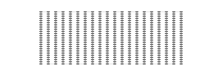
(a) AR(1)

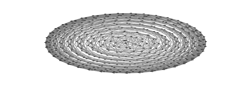
(b) AR(4)

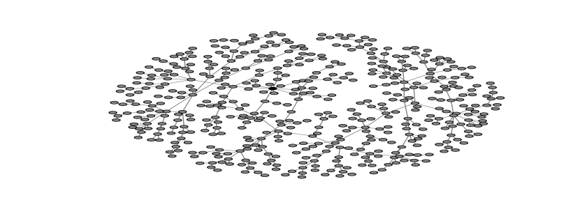
(c) SF

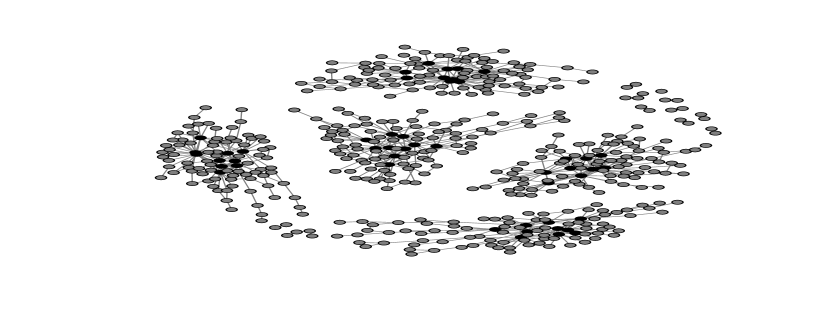
(d) Hub

Figure 3: Four network structures of precision matrix: (a) AR(1), (b) AR(4), (c) Scale-free (SF), and (d) Hub-network (Hub). Nodes in black denote nodes whose degrees are more than 9.

For comparison of the computational efficiency, we consider the number of variables $p=1000$, and sample size $n=250,500$. To provide a benchmark of the computational efficiency, we also consider the well-known existing methods such as the CLIME (Cai et al., 2011b), graphical lasso (GLASSO) (Friedman et al., 2008), and convex partial correlation estimation method (CONCORD) (Khare et al., 2015). As the computation times of the algorithms are affected by the level of sparsity on the estimate of the precision matrix, we set $\lambda_{0}=\sqrt{4n^{-1}\log p}$ for LARS-CPU (SPMESL-LARS) and CD-CPU (SPMESL-CD). Further, we search the tuning parameters for other methods to obtain the level of sparsity similar to the one obtained by the SPMESL. For example, for AR(1) and AR(4) networks with $p=1000$, the averages of the estimated edges of all methods are around 1000, which is $0.2$% of the total possible edges. With the chosen penalty levels, the computation time for each method is measured in CPU time (seconds) by using a workstation (Intel(R) Xeon(R) W-2175 CPU (base: 2.50 GHz, max-turbo: 4.30 GHz) and 128 GB RAM) with NVIDIA GeForce GTX 1080 Ti. We measure the average computation times and standard errors over 10 datasets.

For comparison of the estimation performance, we consider evaluating the estimation performance of the SPMESL with $\lambda_{pb}=\sqrt{2}L_{n}(k/p)$, $\lambda_{univ}=\sqrt{2n^{-1}\log(p-1)}$, and $\lambda_{ub}=\sqrt{4n^{-1}\log p}$ as there are three different suggestions for $\lambda_{0}$ without a comparison of the estimation performance, where $k$ is a real solution of $k=L_{1}^{4}(k/p)+2L_{1}^{2}(k/p)$, $L_{n}(t)=n^{-1/2}\Phi^{-1}(1-t)$, and $\Phi^{-1}(t)$ is the standard normal quantile function. Here, we denote the SPMESL with $\lambda_{pb}$, $\lambda_{univ}$, $\lambda_{ub}$ as SPMESL-P, SPMESL-2, SPMESL-4, respectively. As described in the computational efficiency comparison, we apply the three existing methods (CLIME, GLASSO, CONCORD) to provide a benchmark of the estimation performance. Hereafter, we referred these three methods to the tuning-search methods. To measure the estimation performance, we consider five performance measures– sensitivity (SEN), specificity (SPE), false discovery rate (FDR), miss-classification error rate (MISR), and Matthew’s correlation coefficients (MCC)–for identifying the true edges and the Frobenius norm of $\boldsymbol{\Omega}^{0}-\hat{\boldsymbol{\Omega}}$ for estimation error, where $\boldsymbol{\Omega}^{0}$ and $\hat{\boldsymbol{\Omega}}$ denote the true precision matrix and the estimate of the precision matrix, respectively. The five performance measures for identification of the true edges are defined as follows:

$$\begin{array}[]{l}\vskip 6.0pt plus 2.0pt minus 2.0pt{\rm SEN}\equiv\displaystyle\frac{\rm TP}{({\rm TP}+{\rm FN})},{\rm SPE}\equiv\displaystyle\frac{{\rm TN}}{({\rm TN}+{\rm FP})},{\rm FDR}\equiv\displaystyle\frac{{\rm FP}}{({\rm TP}+{\rm FP})},\\ \vskip 6.0pt plus 2.0pt minus 2.0pt{\rm MISR}\equiv\displaystyle\frac{({\rm FP}+{\rm FN})}{p(p-1)/2},~{}{\rm MCC}(\hat{\Omega},\Omega^{0})\equiv\frac{{\rm TP}\times{\rm TN}-{\rm FP}\times{\rm FN}}{\sqrt{({\rm TP}+{\rm FP})({\rm TP}+{\rm FN})({\rm TN}+{\rm FP})({\rm TN}+{\rm FN})}},\end{array}$$

where ${\rm TP}=\sum_{j<k}I(\hat{\omega}_{jk}\neq 0,\omega^{0}_{jk}\neq 0)$, ${\rm FP}=\sum_{j<k}I(\hat{\omega}_{jk}\neq 0,\omega^{0}_{jk}=0)$, ${\rm TN}=\sum_{j<k}I(\hat{\omega}_{jk}=0,\omega^{0}_{jk}=0)$, and ${\rm FN}=\sum_{j<k}I(\hat{\omega}_{jk}=0,\omega^{0}_{jk}\neq 0)$,

In the comparison of the estimation performance, we set the number of variables and sample size as 500 and 250, respectively. We generate samples ${\bf X}^{1},{\bf X}^{2},\ldots,{\bf X}^{n}\sim N({\bf 0},\boldsymbol{\Sigma})$, where $\boldsymbol{\Sigma}=\boldsymbol{\Omega}^{-1}$ and $\boldsymbol{\Omega}$ is from a given network structure. Unlike the comparison of computational efficiency, we need to choose criteria for the selection of the optimal tuning parameter of the CLIME, GLASSO, and CONCORD. For a fair comparison, we adopt the Bayesian information criterion (BIC), which is widely used in model selection, and search the optimal tuning parameter over an equally spaced grid $(0.10,0.12,\ldots,0.88,0.90)$. We generate 50 datasets, each of which we search the optimal tuning parameters for the CLIME, GLASSO, and CONCORD and apply $\lambda_{pb}$, $\lambda_{univ}$, $\lambda_{ub}$ for the SPMESL.

In this numerical study, we implement R package cdscalreg for the CD algorithm with a warm start strategy for the scaled Lasso and SPMESL, which is available at https://sites.google.com/view/seunghwan-lee/software. For the other methods in this study, we use R packages fastclime for FASTCLIME, glasso for GLASSO, gconcord for CONCORD, scalreg for the original algorithm for SPMESL. Note that consider FASTCLIME (Pang et al., 2014) for the CLIME, which obtains the CLIME estimator efficiently and provides a solution path of the CLIME applying the parametric simplex method. It is also worth noting that the GPUs we used are more efficient for conducting operations with single-precision values than double-precision values, but the R programming language only supports the double-precision that makes the efficiency of the GPU-parallel computation decrease. Although this PCD implementation could decrease its computational efficiency, we develop an R function for the PCD algorithm to provide an efficient and convenient tool for R users. If readers want to utilize GPU-parallel computation maximally, PyCUDA (Klöckner et al., 2012) is one of the convenient and favorable ways to implement CUDA GPU-parallel computation.

4.2 Comparison results for computational efficiency

Table 1 reports the average computation times and standard errors over 10 datasets. From Table 1, we numerically verify that the proposed algorithm based on the CD with warm-start strategy is more efficient than the original algorithm based on the LARS, where the proposed algorithm (CD-CPU) is 110.2 and 466.3 times faster than LARS-CPU for the worst case (AR(1), $n=250$) and the best case (AR(4), $n=500$), respectively. For comparison of efficiency with other methods, overall, the CD-CPU is faster than FASTCLIME and slower than GLASSO and CONCORD. GLASSO is the most efficient algorithm in our numerical study. Its efficiency is from the sub-procedure that reduces the computational cost by the pre-identification procedure for nonzero block diagonals of the estimate that rearranges the order of variables for a given tuning parameter described in Witten et al. (2011). The CONCORD is faster than the CD-CPU in general because the CD algorithm for the CONCORD is applied to minimize its objective function directly. However, the CD algorithm in the CD-CPU is repeatedly applied to solve the lasso subproblems. Even though the GLASSO and CONCORD are faster than the CD-CPU, the GLASSO and CONCORD are tuning-search methods while the CD-CPU is not. Thus, the CD-CPU becomes the most efficient when the GLASSO and CONCORD need to evaluate more than five tuning parameters. For the efficiency of the PCD-GPU, we can see that the PCD-GPU is faster than CD-CPU for all cases except for the case of (Hub, $n=250$). In addition, Table 1 also shows that the efficiency of the PCD-GPU increases as the sample size increases. For example, all computation times of CD-CPU significantly increase when the sample size increases from 250 to 500. However, there is no significant difference on the computation times of PCD-GPU between the sample sizes 250 and 500. This might show that the GPU device has idle processing units when $n=250$. Note that the estimator of the SPMESL can be obtained by solving $p$ scaled Lasso problems independently on multi CPU cores instead of on GPUs. However, the cost per core of CPU is more expensive than that of GPU. Moreover, the average computation times of the parallel computation of the CD-CPU with 16 CPU cores with the R package doParallel (PCD-MPI in Table 1) are around 20 seconds, which are worse than CD-CPU. This inefficiency might be from the communication cost and the number of CPU cores not enough for large $p$.

To verify the efficiency of PCD-GPU compared to CD-CPU, we conduct additional numerical studies for CD-CPU and PCD-GPU with $p=500,1000,2000,5000$ and $n=250,500,1000$. Table 2 reports the average computation times and standard errors measured in CPU time (seconds) for CD-CPU and PCD-GPU. As shown in Table 2, PCD-GPU becomes more efficient than CD-CPU when either the number of variables or the sample size increases. For example, CD-CPU is 1.05$\sim$1.94 times faster than PCD-GPU only for the Hub-network cases of $(p,n)=(500,250),(500,500),(1000,250)$; however, PCD-GPU outperforms CD-CPU for all the other cases and 4.71$\sim$11.65 times faster than CD-CPU when $p=5000$. In Table 2, we also find an advantage of the GPU-parallel computation. Originally, the parallel computation in PCD-GPU applied to reduce the computational cost depends on the number of variables. However, the additional numerical studies support that the parallel computation in PCD-GPU also reduces the computation times when the number of samples increases for a fixed $p$. This advantage is from the efficiency of the GPU-parallel computation for the matrix-matrix and matrix-vector multiplications. Thus, the additional numerical studies show that PCD-GPU is favorable for the cases where either $p$ or $n$ is sufficiently large.

Table 1: The averages of the computation times (sec.) over 10 datasets. Numbers in the parentheses denote the standard errors.

Network	$p$	$n$	scalreg	CD-CPU	PCD-GPU	PCD-MPI	FASTCLIME	GLASSO	CONCORD
AR(1)	1000	250	937.7358	8.5027	4.4356	18.8599	241.0991	0.7091	6.4348
			(4.4662)	(0.0519)	(0.0749)	(0.7913)	(4.0303)	(0.0081)	(0.1541)
		500	4345.7155	13.9459	4.2743	21.4523	227.3807	1.2521	12.4249
			(3.9313)	(0.0335)	(0.0397)	(0.8523)	(2.2561)	(0.1210)	(0.0830)
AR(4)	1000	250	803.3684	5.9992	1.7896	19.2027	233.5897	0.8030	3.4643
			(0.9841)	(0.0158)	(0.0274)	(1.0094)	(1.9512)	(0.0460)	(0.0410)
		500	4043.0187	8.6698	2.2892	20.0631	259.5524	8.9721	7.5435
			(4.4534)	(0.0220)	(0.0317)	(0.8708)	(2.0104)	(0.2280)	(0.2210)
Scale-Free	1000	250	790.8713	5.1367	3.0949	18.8765	238.7474	0.6852	3.5295
			(0.6122)	(0.0376)	(0.0545)	(1.3815)	(1.7989)	(0.0010)	(0.0481)
		500	3819.9712	9.1574	3.0781	19.2749	246.0107	0.7945	7.0473
			(8.2088)	(0.0190)	(0.0255)	(0.7189)	(1.2268)	(0.0014)	(0.0775)
Hub	1000	250	787.6731	4.7785	7.3326	18.8566	245.2853	0.7512	6.1875
			(0.8286)	(0.0247)	(0.1355)	(1.3197)	(1.6676)	(0.0099)	(0.1024)
		500	3769.7531	9.2215	7.7584	18.7167	250.2303	2.2454	12.7924
			(23.6487)	(0.0458)	(0.1942)	(0.5727)	(2.0064)	(0.1917)	(0.2707)

Table 2: The averages of the computation times (sec.) over 10 datasets. Numbers in the parentheses denote the standard errors.

Network	$n$	$p=500$		$p=1000$		$p=2000$		$p=5000$
		CD	PCD	CD	PCD	CD	PCD	CD	PCD
AR(1)	250	2.2800	1.9528	8.7067	4.4149	38.1056	12.0651	297.7769	60.1581
		(0.0224)	(0.0414)	(0.0268)	(0.0765)	(0.0841)	(0.1121)	(0.2836)	(0.9851)
	500	3.4519	1.7117	13.8964	4.2744	59.2341	12.8309	436.7230	64.4670
		(0.0134)	(0.0330)	(0.0419)	(0.0445)	(0.0736)	(0.1152)	(2.7395)	(0.7545)
	1000	5.8935	1.7364	23.5556	4.9784	99.7887	15.8946	700.8538	85.5756
		(0.0265)	(0.0217)	(0.0636)	(0.0561)	(0.1460)	(0.1447)	(1.0246)	(0.6645)
AR(4)	250	1.4538	0.8794	6.1486	1.7679	27.9208	4.9945	232.7940	20.9527
		(0.0077)	(0.0258)	(0.0265)	(0.0271)	(0.0666)	(0.2905)	(0.2484)	(0.3062)
	500	2.1363	0.9950	8.5920	2.2517	37.8047	6.2053	305.4613	26.2313
		(0.0116)	(0.0177)	(0.0254)	(0.0372)	(0.0777)	(0.2523)	(0.3319)	(0.6105)
	1000	6.1868	1.5552	21.5172	4.1366	80.3323	12.1282	499.1462	57.1606
		(0.0312)	(0.0155)	(0.1308)	(0.0284)	(0.3212)	(0.0558)	(2.8728)	(0.7015)
Scale-Free	250	1.2493	1.1620	4.9605	2.9021	22.1757	6.8921	186.5103	35.0760
		(0.0067)	(0.0328)	(0.0227)	(0.0426)	(0.0362)	(0.0762)	(0.2680)	(0.6203)
	500	2.1820	1.1572	8.7524	2.9931	38.4489	8.3851	300.9288	44.9643
		(0.0094)	(0.0109)	(0.0196)	(0.0276)	(0.0646)	(0.1162)	(0.6319)	(0.5134)
	1000	3.7781	1.2210	15.0969	3.6376	65.1003	11.1231	479.8427	63.4638
		(0.0074)	(0.0122)	(0.0141)	(0.0298)	(0.1194)	(0.0762)	(1.4722)	(0.9511)
Hub	250	1.2021	2.3266	4.5724	6.9508	19.9179	11.6372	168.9348	35.8963
		(0.0075)	(0.0434)	(0.0207)	(0.1257)	(0.0456)	(0.2135)	(0.2214)	(0.6634)
	500	2.2632	2.3915	8.9738	7.6092	38.4337	15.7290	300.2697	53.2606
		(0.0078)	(0.0335)	(0.0220)	(0.1866)	(0.0630)	(0.3070)	(0.4684)	(0.4222)
	1000	3.9263	2.6366	15.6040	9.6065	66.8115	21.4761	492.7247	77.6366
		(0.0108)	(0.0342)	(0.0279)	(0.1127)	(0.1204)	(0.1523)	(1.1698)	(0.4552)

4.3 Comparison results for estimation performance

Tables 3 and 4 report the averages of the number of estimated edges ($|\hat{E}|$) and the six performance measures over 50 data sets for AR(1), AR(4), Scale-free, and Hub networks. From the results in Tables 3 and 4, we can find several interesting features. First, focusing on comparing SPMESL-P, SPMESL-2, and SPMESL-4, the SPMESL-P obtains the smallest estimation error in Frobenius norm, and the SPMESL-4 has the largest estimation error for all network structures. The estimation error of SPMESL-2 is located near the middle of an interval defined by the estimation errors of the SPMESL-P and SPMESL-4. However, for the performance in the identification of the true edges, the SPMESL-4 has the smallest SEN and FDR for all network structures, and the SPMESL-2 obtains the lowest MISR and the highest MCC for Scale-free and Hub networks while the SPMESL-P has the highest MISR and the lowest MCC for all network structures. For AR(1) and AR(4) network structures, the MISR and the MCC of the SPMESL-2 are worse than those of the SPMESL-4, but the differences of the SPMESL-2 and the SPMESL-4 are small. For example, the difference in the MCC of the SPMESL-2 and the SPMESL-4 are 0.0195 and 0.0095 in an original scale for AR(1) and AR(4), respectively.

Second, by comparing the SPMESL and the tuning-search methods (CLIME, GLASSO, CONCORD), the SPMESL-2 and SPMESL-4 obtain considerably small FDRs compared to the tuning-search methods. For example, the FDRs by the tuning-search methods are over 27% for all cases, but the FDRs by the SPMESL-2 and the SPMESL-4 are less than 6.2%. The SPMESL-P has the lowest MCC and the highest FDR for Scale-free and Hub networks and obtains the second-lowest MCC and the second-highest FDR for AR(4) networks, where only the GLASSO is worse than the SPMESL-P in terms of the MCC and FDR. For AR(1) network, the SPMESL with all penalty levels are better than the tuning-search methods for identifying the true edges, and the estimation errors of the SPMESL-P and SPMESL-2 are less than those of the tuning-search methods.

Finally, we compare the estimation performance of the tuning-search methods. For the estimation error in the Frobenius norm, the CONCORD outperforms CLIME and GLASSO for all cases, where the CONCORD obtains similar estimation errors to the SPMESL-P for AR(4), Scale-free, and Hub networks. However, for the identification of the true edges, the CLIME obtains slightly better performance than the CONCORD for all networks except the AR(1) network. For the AR(1) network, the CONCORD outperforms CLIME and GLASSO for estimation error and identification of the true edges. In our numerical study, the CONCORD is favorable among the three tuning-search methods we consider. Note that we adopt the BIC for three tuning-search methods for a fair comparison, but the comparison results might be changed if we apply other model selection criteria.

From the results of the estimation performance comparison, we recommend the SPMESL with the universal penalty level $\lambda_{univ}$ if the target problem can accept the FDR level around 5%; the uniform-bound penalty level is only preferred when the problem only accepts the small FDR less than 1%. Note that we do not recommend using the probabilistic bound $\lambda_{pb}$ as the SPMESL-P has the highest FDR among three penalty levels for the SPMESL, which are over 50% for Scale-free and Hub networks, although the SPMESL-P obtains the lowest estimation error in Frobenius norm.

Table 3: For AR(1) and AR(4) networks with $p=500$ and $n=250$, the averages of the number of estimated edges, the five performance measures and the Frobenius norms of difference of the estimate and true precision matrix over 50 datasets. Numbers in the parentheses denote the standard errors.

Network	Method	$|\hat{E}|$	SEN	SPE	FDR	MISR	MCC	$\|\hat{\Omega}-\Omega\|_{F}$
	CLIME	897.80	100.00	99.68	44.33	0.32	74.48	9.17
		(5.20)	(0.00)	(0.00)	(0.31)	(0.00)	(0.21)	(0.02)
	GLASSO	2134.48	100.00	98.68	76.57	1.31	48.07	12.74
		(14.52)	(0.00)	(0.01)	(0.16)	(0.01)	(0.17)	(0.02)
	CONCORD	722.16	100.00	99.82	30.84	0.18	83.08	4.96
AR(1)		(2.93)	(0.00)	(0.00)	(0.29)	(0.00)	(0.17)	(0.01)
$(|E|=499)$	SPMESL-P	649.28	100.00	99.88	23.12	0.12	87.62	3.65
		(1.68)	(0.00)	(0.00)	(0.20)	(0.00)	(0.11)	(0.01)
	SPMESL-2	524.74	100.00	99.98	4.90	0.02	97.51	4.55
		(0.77)	(0.00)	(0.00)	(0.14)	(0.00)	(0.07)	(0.01)
	SPMESL-4	504.40	100.00	100.00	1.07	0.00	99.46	6.39
		(0.36)	(0.00)	(0.00)	(0.07)	(0.00)	(0.04)	(0.01)
	CLIME	908.58	32.55	99.79	28.70	1.29	47.65	22.35
		(2.66)	(0.08)	(0.00)	(0.15)	(0.00)	(0.08)	(0.01)
	GLASSO	988.96	28.86	99.66	41.66	1.47	40.36	23.17
		(10.79)	(0.07)	(0.01)	(0.52)	(0.01)	(0.17)	(0.01)
	CONCORD	979.40	33.03	99.74	32.86	1.33	46.52	18.46
AR(4)		(3.33)	(0.08)	(0.00)	(0.19)	(0.00)	(0.10)	(0.01)
$(|E|=1990)$	SPMESL-P	1206.32	36.31	99.61	40.09	1.40	45.99	18.40
		(2.97)	(0.07)	(0.00)	(0.16)	(0.00)	(0.09)	(0.01)
	SPMESL-2	545.30	25.71	99.97	6.18	1.21	48.77	20.57
		(0.94)	(0.02)	(0.00)	(0.15)	(0.00)	(0.05)	(0.01)
	SPMESL-4	499.00	25.05	100.00	0.11	1.20	49.72	22.72
		(0.17)	(0.01)	(0.00)	(0.02)	(0.00)	(0.01)	(0.01)

Table 4: For Scale-Free and Hub networks with $p=500$ and $n=250$, the averages of the number of estimated edges, the five performance measures and the Frobenius norms of differences of the estimate and true precision matrix over 50 datasets. Numbers in the parentheses denote the standard errors.

Network	Method	$|\hat{E}|$	SEN	SPE	FDR	MISR	MCC	$\|\hat{\Omega}-\Omega\|_{F}$
	CLIME	643.08	91.38	99.85	29.63	0.19	80.10	8.33
		(2.19)	(0.16)	(0.00)	(0.24)	(0.00)	(0.17)	(0.01)
	GLASSO	810.52	92.84	99.72	43.08	0.31	72.53	7.79
		(7.21)	(0.19)	(0.01)	(0.52)	(0.01)	(0.31)	(0.02)
	CONCORD	682.36	93.04	99.82	32.39	0.21	79.20	5.33
Scale-Free		(4.00)	(0.17)	(0.00)	(0.40)	(0.00)	(0.23)	(0.01)
$(|E|=495)$	SPMESL-P	1022.56	94.60	99.55	54.18	0.47	65.66	5.15
		(3.66)	(0.14)	(0.00)	(0.17)	(0.00)	(0.14)	(0.01)
	SPMESL-2	457.88	87.94	99.98	4.92	0.07	91.40	6.57
		(1.06)	(0.15)	(0.00)	(0.16)	(0.00)	(0.11)	(0.01)
	SPMESL-4	348.34	70.33	100.00	0.06	0.12	83.79	8.83
		(0.85)	(0.17)	(0.00)	(0.02)	(0.00)	(0.10)	(0.01)
	CLIME	644.02	84.36	99.86	27.80	0.21	77.93	8.43
		(2.31)	(0.23)	(0.00)	(0.21)	(0.00)	(0.17)	(0.01)
	GLASSO	881.76	87.44	99.68	45.03	0.38	69.10	7.89
		(10.37)	(0.27)	(0.01)	(0.59)	(0.01)	(0.31)	(0.02)
	CONCORD	731.22	89.03	99.81	32.73	0.24	77.24	5.55
Hub		(5.43)	(0.19)	(0.00)	(0.51)	(0.00)	(0.27)	(0.01)
$(|E|=551)$	SPMESL-P	1094.14	91.32	99.52	53.99	0.51	64.62	5.37
		(3.33)	(0.14)	(0.00)	(0.14)	(0.00)	(0.12)	(0.01)
	SPMESL-2	474.36	81.22	99.98	5.64	0.10	87.49	6.78
		(1.55)	(0.22)	(0.00)	(0.15)	(0.00)	(0.13)	(0.01)
	SPMESL-4	319.72	57.96	100.00	0.11	0.19	76.02	8.90
		(1.20)	(0.21)	(0.00)	(0.02)	(0.00)	(0.14)	(0.01)

5 Conclusion

In this paper, we proposed an efficient coordinate descent algorithm with the warm start strategy for sparse precision matrix estimation using the scaled lasso motivated by the empirical observation that the iterative solution for the diagonal elements of the precision matrix needs only a few iterations. In addition, we also develop the parallel coordinate descent algorithm (PCD) for the SPMESL by representing $p$ Lasso subproblems as the unified minimization problem. In the PCD algorithm, we use a different convergence criterion $\|{\bf B}^{(k+1)}-{\bf B}^{(k)}\|_{\infty}<\delta$ to check the convergence of the PCD algorithm for the unified minimization problem. We show that the difference in the iterative solutions of the CD and PCD caused by the difference of the convergence criteria is also bounded by the convergence tolerance $\delta$.

Our numerical study shows that the proposed CD algorithm is much faster than the original algorithm of the SPMESL, which adopts the LARS algorithm to solve the Lasso subproblems. Moreover, the PCD algorithm with GPU-parallel computation becomes more efficient than the CD algorithm when either the number of variables or the sample size increases. For the optimal tuning parameter for the SPMESL, there are three suggestions without the comparison of the estimation performance. In the additional simulation, we numerically investigate the estimation performance of the SPMESL with the three penalty levels and the other three tuning-search methods. From the comparison results, the SPMESL with the uniform bound level and the universal penalty level outperform the three tuning-search methods. Specifically, the probabilistic bound level $\lambda_{pb}=\sqrt{2}L_{n}(k/p)$ provides the estimate that has the smallest estimation error in terms of the Frobenius norm; the uniform bound level $\lambda_{ub}=\sqrt{4n^{-1}\log(p)}$ provides the estimate that has the smallest FDR less than 1%; and the universal penalty level $\lambda_{univ}=\sqrt{2n^{-1}\log(p-1)}$ obtains either the best or second-best in terms of MCC and FDR. Overall, we recommend the SPMESL with the universal penalty level and apply the CD algorithm if $p$ is less than or equal to $1000$ and the PCD algorithm when the target problem has more than 1000 variables and GPU-parallel computation is available.

Acknowlegements

Sang Cheol Kim’s research was supported by funding (2019-NI-092-00) from the Research of Korea Centers for Disease Control and Prevention. Donghyeon Yu’s research was supported by the INHA UNIVERSITY Research Grant and the National Research Foundation of Korea (NRF-2020R1F1A1A01048127).

References

- Ali et al. (2017) Ali, A., Khare K., Oh S.-Y., and Rajaratnam, B. (2017). Generalized pseudolikelihood methods for inverse covariance estimation. Proceedings of the 20th International Conference on Artificial Intelligence and Statistics, 54, 280–288.
- Barabási and Albert (1999) Barabási, A. and Albert, R. (1999). Emergence of scaling in random networks. Science, 286, 509–512. doi:10.1126/science.286.5439.509
- Bickel and Levina (2008a) Bickel, P. J. and Levina, E. (2008a). Regularized estimation of large covariance matrices. The Annals of Statistics, 36, 199–227. doi:10.1214/009053607000000758
- Bickel and Levina (2008b) Bickel, P. J. and Levina, E. (2008b). Covariance regularization by thresholding. The Annals of Statistics, 36, 2577–2604. doi:10.1214/08-AOS600
- Cai et al. (2010) Cai, T. T., Zhang, C. H., and Zhou H. H. (2010). Optimal rates of convergence for covariance matrix estimation. The Annals of Statistics, 38, 2118–2144. doi:10.1214/09-AOS752
- Cai and Liu (2011a) Cai, T. and Liu, W. (2011a). Adaptive thresholding for sparse covariance matrix estimation. Journal of the American Statistical Association,106, 672–684. https://doi.org/10.1198/jasa.2011.tm10560
- Cai et al. (2011b) Cai, T. T., Liu, W. and Luo, X. (2011b). A constrained minimization approach to sparse precision matrix estimation. Journal of the American Statistical Association, 106, 594–607. https://doi.org/10.1198/jasa.2011.tm10155
- Cai and Zhou (2012) Cai, T. T. and Zhou, H. H. (2012). Minimax estimation of large covariance matrices under norm. Statistica Sinica, 22, 1319–1349. http://dx.doi.org/10.5705/ss.2010.253
- Cai et al. (2016) Cai, T. T., Liu, W., and Zhou, H. H. (2016). Estimating sparse precision matrix: optimal rates of convergence and adaptive estimation, The Annals of Statistics, 44, 455–488. doi:10.1214/13-AOS1171
- Efron et al. (2004) Bradely Efron, B., Hastie, T., Johnstone, I., and Tibshirani, R. (2004). Least angle regression. The Annals of Statistics, 32, 407–499. doi:10.1214/009053604000000067
- Friedman et al. (2008) Friedman, J., Hastie, T. and Tibshirani, R. (2008). Sparse inverse covariance estimation with the graphical Lasso. Biostatistics, 9, 432-–441. https://doi.org/10.1093/biostatistics/kxm045
- Khare et al. (2015) Khare, K., Oh, S.-Y., and Rajaratnam, B. (2015). A convex pseudolikelihood framework for high dimensional partial correlation estimation with convergence guarantees. Journal of the Royal Statistical Society: Series B, 77, 803–825. http://www.jstor.org/stable/24775310
- Klöckner et al. (2012) Klöckner, A., Pinto, N., Lee, Y., Catanzaro, B., Ivanov, P., and Fasih, A. (2012). PyCUDA and PyOpenCL: A scripting-based approach to GPU run-time code generation, Parallel Computing, 38, 157–174. https://doi.org/10.1016/j.parco.2011.09.001
- Mazumder et al. (2012) Mazumder, R. and Hastie, T. (2012). The graphical lasso: New insights and alternatives. Electronic Journal of Statistics, 6, 2125–2149. doi:10.1214/12-EJS740
- Meinshausen and Bühlmann (2006) Meinshausen, N. and Bühlmann, P. (2006). High dimensional graphs and variable selection with the Lasso. The Annals of Statistics, 34, 1436–1462. doi:10.1214/009053606000000281
- Pang et al. (2014) Pang, H., Liu, H., and Vanderbei, R. (2014). The FASTCLIME package for linear programming and large-scale precision matrix estimation in R. Journal of Machine Learning Research, 15, 489–493.
- Peng et al. (2009) Peng, J., Wang, P., Zhou, N., and Zhu, J. (2009). Partial correlation estimation by joint sparse regression models. Journal of the American Statistical Association, 104, 735–746. doi:10.1198/jasa.2009.0126
- Ren et al. (2015) Ren, Z., Sun, T., Zhang, C.-H., and Zhou H. H. (2015). Asymptotic normality and optimalities in estimation of large Gaussian graphical model. The Annals of Statistics, 43, 991–1026. doi:10.1214/14-AOS1286
- Rothman et al. (2009) Rothman, A. J., Levina, E. and Zhu, J. (2009). Generalized thresholding of large covariance matrices. Journal of the American Statistical Association, 104, 177–186. https://doi.org/10.1198/jasa.2009.0101
- Schäfer and Strimmer (2005) Schäfer, J., and Strimmer, K. (2005). A shrinkage approach to large-scale covariance matrix estimation and implications for functional genomics. Statistical Applications in Genetics and Molecular Biology, 4, 32. https://doi.org/10.2202/1544-6115.1175
- Sun and Zhang (2012) Sun, T. and Zhang, C. H. (2012). Scaled sparse linear regression. Biometrika, 99, 879–898. doi:10.1093/biomet/ass043
- Sun and Zhang (2013) Sun, T. and Zhang, C. H. (2013). Sparse matrix inversion with scaled lasso Journal of Machine Learning Research, 14, 3385–3418.
- Tibshirani (1996) Tibshirani, R. (1996). Regression shrinkage and selection via the Lasso. Journal of the Royal Statistical Society Series B, 58, 267–288. https://doi.org/10.1111/j.2517-6161.1996.tb02080.x
- Tseng (2001) Tseng, P. (2001). Convergence of a block coordinate descent method for nondifferentiable minimization. Journal of Optimization Theory and Applications, 109, 475–494. https://doi.org/10.1023/A:1017501703105
- van de Geer and Bühlmann (2009) van de Geer, S. and Bühlmann, P. (2009). On the conditions used to prove oracle results for the Lasso. Electronic Journal of Statistics, 3, 1360–1392. doi:10.1214/09-EJS506
- Witten et al. (2011) Witten, D., Friedman, J., and Simon, N. (2011). New insights and faster computations for the graphical lasso. Journal of Computational and Graphical Statistics, 20, 892–900. https://doi.org/10.1198/jcgs.2011.11051a
- Wu and Lange (2008) Wu, T. T. and Lange, K. (2008). Coordinate descent algorithms for lasso penalized regression. Annals of Applied Statistics, 2, 224–244. doi:10.1214/07-AOAS147
- Wu et al. (2009) Wu, W. B. and M. Pourahmadi (2009). Banding sample autocovariance matrices of stationary processes. Statistica Sinica, 19, 1755–1768.
- Yao et al. (2015) Yao, J., Zheng, S., and Bai, Z. (2015). Large sample covariance matrices and high-dimensional data analysis, New York, NY: Cambridge University Press. https://doi.org/10.1017/CBO9781107588080
- Yuan and Lin (2007) Yuan, M. and Y. Lin (2007). Model selection and estimation in the Gaussian graphical model. Biometrika, 94, 19–35. https://doi.org/10.1093/biomet/asm018
- Yuan (2010) Yuan, M. (2010). Sparse inverse covariance matrix estimation via linear programming. The Journal of Machine Learning Research, 11, 2261–2286.