Solving Disjunctive Temporal Networks with Uncertainty under Restricted Time-Based Controllability using Tree Search and Graph Neural Networks

Abstract

Planning under uncertainty is an area of interest in artificial intelligence. We present a novel approach based on tree search and graph machine learning for the scheduling problem known as Disjunctive Temporal Networks with Uncertainty (DTNU). Dynamic Controllability (DC) of DTNUs seeks a reactive scheduling strategy to satisfy temporal constraints in response to uncontrollable action durations. We introduce new semantics for reactive scheduling: Time-based Dynamic Controllability (TDC) and a restricted subset of TDC, R-TDC. We design a tree search algorithm to determine whether or not a DTNU is R-TDC. Moreover, we leverage a graph neural network as a heuristic for tree search guidance. Finally, we conduct experiments on a known benchmark on which we show R-TDC to retain significant completeness with regard to DC, while being faster to prove. This results in the tree search processing fifty percent more DTNU problems in R-TDC than the state-of-the-art DC solver does in DC with the same time budget. We also observe that graph neural network search guidance leads to substantial performance gains on benchmarks of more complex DTNUs, with up to eleven times more problems solved than the baseline tree search.

1 Introduction and Related Works

Temporal Networks (TN) are a common formalism to represent temporal constraints over a set of time points (e.g. start/end of activities in a scheduling problem). The Simple Temporal Network with Uncertainty (STNUs) introduced by Vidal and Fargier (1999) explicitly incorporates qualitative uncertainty into temporal networks. Applications include control of robotic systems such as in Bhargava et al. (2018) and Stegun, Chien, and Agrawal (2020), with limited ethical concerns thus far. Considerable work has resulted in algorithms to determine whether or not all timepoints can be scheduled, either up-front or reactively, in order to account for uncertainty (e.g. Morris and Muscettola (2005), Morris (2014)). Dynamic Controllability (DC) is a form of scheduling in which a controller agent integrates observed events as they unfold to adapt the scheduling reactively. In particular, an STNU is said to be DC if there is a reactive scheduling strategy in which controllable timepoints can be executed either at a specific time, or after observing the occurrence of an uncontrollable timepoint. Cimatti, Micheli, and Roveri (2016) investigate the problem of DC for Disjunctive Temporal Networks with Uncertainty (DTNUs), which generalize STNUs. Figure 1a shows two DTNUs $\gamma$ and $\gamma^{\prime}$ on the left side; $a_{i}$ are controllable timepoints, $u_{j}$ are uncontrollable timepoints. Timepoints are variables which can take on any value in $\mathbb{R}$. Constraints between timepoints characterize a minimum and maximum time distance separating them, likewise valued in $\mathbb{R}$. The key difference between STNUs and DTNUs lies in the disjunctions that yield more choice points for consistent scheduling, especially reactively (e.g. if an uncontrollable timepoint occurs early, a given constraint could be satisfied, if it occurs late, another one, linked by a disjunction, could be).

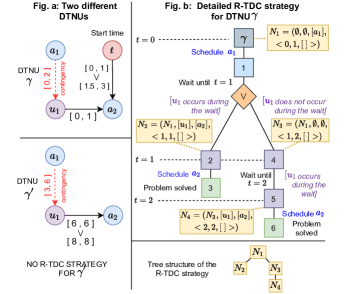
Figure 1: Two example DTNUs $\gamma$ and $\gamma^{\prime}$. Timepoints $a_{1}$ and $a_{2}$ are controllable; $u_{1}$ uncontrollable. Black arrows represent time constraints between timepoints; red arrows contingency links. A detailed R-TDC strategy is displayed for $\gamma$. Squares below $\gamma$ are sub-DTNUs; the $\lor$ sign lists transitional possibilities. Nodes $N_{i}$ are R-TDC strategy nodes.

DC-checking for STNUs is $\mathcal{O}(N^{3})$ (Morris (2014)), however, it is $PSPACE$-complete for DTNUs (Bhargava and Williams (2019a)), making this a highly challenging problem. The difficulty in proving or disproving DC arises from the need to check all possible combinations of disjuncts to handle all possible outcomes of uncontrollable timepoints. DTNUs are nonetheless more expressive than STNUs, and many real world applications require time-windows in which certain tasks can be scheduled either in a given interval or another, making it a problem worth studying. The best previously published approaches for this problem come from Cimatti, Micheli, and Roveri (2016) and use timed-game automata and satisfiability modulo theories.

An emerging trend of neural networks, Graph Neural Networks (GNNs), has been proposed to extend convolutional neural networks (Krizhevsky, Sutskever, and Hinton (2012)) to graph inputs for machine learning tasks. Recent variants based on spectral graph theory include works from Defferrard, Bresson, and Vandergheynst (2016) and Kipf and Welling (2017). They leverage relational properties between nodes, but do not take into account potential edge weights. In newer spatial-based approaches, Message Passing Neural Networks (MPNNs) from Battaglia et al. (2016), Gilmer et al. (2017) and Kipf et al. (2018) use embeddings comprising edge weights within each computational layer. We focus on these architectures as DTNUs can be formalized as graphs with edge distances representing time constraints.

In this work, we pose DC-checking of DTNUs as a search problem, express states as graphs, and use MPNNs to learn heuristics based on previously solved DTNUs to guide search. The key contributions of our approach are the following. (1) We introduce new semantics for reactive scheduling: Time-based Dynamic Controllability (TDC), and a restricted subset of TDC, R-TDC. We present a tree search approach to identify R-TDC strategies. (2) We describe an MPNN architecture trained with self-supervised learning for handling DTNU scheduling problems and use it as heuristic for guidance in the tree search. (3) We carry out experiments on a known benchmark showing that R-TDC retains significant completeness compared to DC while being faster to prove. This leads to $50$% more DTNU instances processed in R-TDC by the tree search than in DC with the state-of-the-art DC solver in the same time budget. Moreover, we show that the learned MPNN heuristic considerably improves the tree search on benchmarks of harder DTNUs: performance gains go up to $11$ times more instances solved than the baseline tree search within the same time frame. Our results also highlight that the MPNN, which is trained on a set of solved DTNUs, is able to generalize to larger DTNUs than those on which it was trained.

2 Problem and Controllability Definitions

We next provide definitions necessary in the context of this work: Dynamic Controllability (DC), Time-based Dynamic Controllability (TDC) and Restricted TDC (R-TDC).

Definition 1 (DTNU and variants).

A DTNU $\Gamma$ is a tuple {A,U,C,L}, where: A is a set of controllable timepoints; U a set of uncontrollable timepoints; C a set of free constraints, each of the form $\lor_{k=1}^{q}v_{k,j}-v_{k,i}\in[x_{k},y_{k}]$, for some $v_{k,j},v_{k,i}\in V=A\cup U$, $x_{k},y_{k}\in\mathbb{R}\cup\{-\infty,+\infty\}$ and $q\in\mathbb{Z}^{+}$; L a set of contingency links, each of the form $\langle a_{i},\lor_{k=1}^{q^{\prime}}[x_{k}^{\prime},y_{k}^{\prime}],u_{j}\rangle$ where $a_{i}\in A$, $u_{j}\in U$, $x_{k}^{\prime},y_{k}^{\prime}\in\mathbb{R}\cup\{-\infty,+\infty\}$, $0\leq x_{k}^{\prime}\leq y_{k}^{\prime}\leq x_{k+1}^{\prime}\leq y_{k+1}^{\prime}~{}\forall k=1,2,...,q^{\prime}-1$ and $q^{\prime}\in\mathbb{Z}^{+}$, indicating possible occurrence time intervals of $u_{j}$ after $a_{i}$. A DTNU without uncontrollable timepoints is referred to as Disjunctive Temporal Network (DTN). STNUs follow the same definition as DTNUs but do not contain any disjunction inside constraints. Finally, an STNU without uncontrollable timepoints is a Simple Temporal Network (STN).

Definition 2 (DC & TDC).

DC is a reactive form of scheduling which incorporates occurrences of uncontrollable events as they unfold and adapts to them. A problem is DC if and only if it admits a valid dynamic strategy expressed as a map from partial schedules to Real-Time Execution Decisions (RTEDs) (Cimatti, Micheli, and Roveri (2016)). A partial schedule represents the current scheduling state, i.e. the set of timepoints that have been scheduled or occurred so far and their timing. RTEDs allow for two possible actions: (1) The wait action, i.e. wait for an uncontrollable timepoint to occur. (2) The $(t,\mathcal{X})$ action, i.e. if nothing happens before time $t$, schedule the controllable timepoints in $\mathcal{X}$ at $t$. A strategy is valid if, for every possible occurrence of the uncontrollable timepoints, controllable timepoints get scheduled in a way that all free constraints are satisfied. A TDC strategy is a representation of a DC strategy as a timed tree, i.e. a map from tree nodes to children nodes. Tree nodes represent partial schedules, and their children lead to the execution of one of the following actions: (1) Schedule a set of controllable timepoints at current time; (2) Wait a period of time or until an uncontrollable timepoint occurs, whichever happens first.

Definition 3 (R-TDC).

R-TDC is a finite subset of TDC. In particular, actions associated to a partial schedule in R-TDC are: (1) Schedule a set of controllable timepoints at current time; (2) Wait an uninterruptible period of time, the wait duration being defined by time discretization rules in § 4.2.

A TDC strategy can fully express a DC strategy which has an infinite number of mappings from partial schedules to RTEDs, given an infinite tree. In this work, we restrict TDC to a finite search space, R-TDC, and weigh how loss of search completeness results in increased efficiency. The restrictions in R-TDC stem from the uninterruptible waits: occurrence times of uncontrollable timepoints happening in waits are only bounded. Thus, partial schedules in R-TDC tree nodes do not carry exact occurrence times for uncontrollable timepoints which already occurred but only occurrence intervals. Moreover, time discretization rules are used in R-TDC to inspect a partial schedule in order to define a wait duration. The aim is to maximize the duration to speed up strategy search while limiting loss of possible strategies. Lastly, in order to improve completeness, we augment R-TDC waits with the possibility of instantaneous reactive executions during strategy execution. These are requests made to the waiting controller agent to immediately execute some controllable timepoint(s) when it observes an uncontrollable timepoint occur. Associated waits remain uninterruptible during strategy search however, resulting in only bounded and not exact scheduling times of controllable timepoints which are executed in such fashion, as shown in Figure 2.

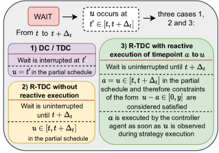
Figure 2: Execution of waits by controllability type. Timepoint $u$ is uncontrollable; $a$ is controllable. A wait from $t$ to $t+\Delta_{t}$ is considered and corresponding behaviors are shown.

Definition 3a (R-TDC strategy structure).

A R-TDC strategy is a finite tree. This tree is comprised of a list of nodes ($N_{1}$,$N_{2}$, …, $N_{q-1}$, $N_{q}$). Each $N_{i}$ is of the form:

$$N_{i}=(N_{j},O_{ji},E_{i},\langle s_{i},e_{i},R_{i}\rangle)$$

where:

• $N_{j}$ is the parent node of $N_{i}$ in the tree.

• Time $s_{i}$ is the start time of the wait in node $N_{i}$.

• Time $e_{i}$ is the end time of the wait in node $N_{i}$.

• $O_{ji}$ is the list of uncontrollable timepoints assumed to occur during the wait in node $N_{j}$. There exist as many $O_{ji}$ as the number of combinations of uncontrollable timepoints that may occur during the wait in node $N_{j}$. Therefore, in a R-TDC strategy, node $N_{j}$ will have exactly the same number of children nodes to account for all possible outcomes of uncontrollable timepoints.

• $R_{i}$ is a mapping which can associate to any uncontrollable timepoint that may occur in the wait $\langle s_{i},e_{i}\rangle$ a set of controllable timepoints to reactively execute by the agent during strategy execution. The associated wait remains uninterrupted during strategy search even if some uncontrollable timepoints are assumed to occur in the wait.

• $E_{i}$ is a set of controllable timepoints to schedule at $s_{i}$.

Each path from the root node of a R-TDC strategy to any leaf node satisfies the following properties:

• It covers the time horizon entirely (each new wait starts at the same time as the end of the previous wait).

• It represents a unique outcome of the occurrence possibilities of uncontrollable timepoints. Each uncontrollable timepoint is bounded in an occurrence interval $\langle s_{i},e_{i}\rangle$. All possible outcomes are included in the strategy.

• It assigns to every controllable timepoint a given time of scheduling (or time interval for those reactively executed in response to uncontrollable timepoints).

• All constraints are satisfied given the scheduling time, scheduling time intervals and occurrence intervals of all timepoints.

We explain next how a R-TDC strategy is executed.

R-TDC Strategy Execution.

A R-TDC strategy is executed in the following way by a controller agent. The agent starts at the root R-TDC node. For each current node $N_{i}=(N_{j},O_{ji},E_{i},\langle s_{i},e_{i},R_{i}\rangle)$, it executes at $t=s_{i}$ the timepoints in $E_{i}$, and waits from time $s_{i}$ to $e_{i}$ with the reactive strategy $R_{i}$, i.e. if $R_{i}$ stipulates it, the agent will immediately execute some controllable timepoints in response to some uncontrollable timepoints that may occur during the wait, as soon as they do. At the end of the wait, the agent deduces from the list of uncontrollable timepoints that occurred which child $N_{i}^{\prime}$ of node $N_{i}$ it transitioned to. It moves to $N_{i}^{\prime}$ and repeats the same process. Those guidelines are followed recursively until all constraints are satisfied.

We give a simple example of a R-TDC strategy for a DTNU $\gamma$ in Figure 1. DTNU $\gamma^{\prime}$ on the other hand is an example of a DTNU which is DC and TDC but not R-TDC. More precisely, it shows a clear limitation of R-TDC: when a controllable timepoint $a$ absolutely has to be scheduled a set time after an uncontrollable timepoint $u$ occurs: $a-u\in[x,x],x\in\mathbb{R}^{+}$. This is impossible in R-TDC as occurrence time of $u$ can only be bounded during strategy search and not exact, because any wait interval, however small, in which $u$ is assumed to occur is bounded.

3 Tree Search Preliminaries

We introduce here the tree search algorithm. The root of the search tree built by the algorithm is a DTNU, and other tree nodes are either sub-DTNUs or logical nodes (OR, AND) which respectively represent decisions that can be made and how uncontrollable timepoints can unfold. At a given DTNU tree node, decisions such as scheduling a controllable timepoint at current time or waiting for a period of time develop children DTNU nodes for which these decisions are propagated to constraints. In this tree, only one timepoint can be scheduled per branch, rather than a set of timepoints, simply for compatibility reasons with the heuristic function used for guidance. The R-TDC controllability of a leaf DTNU node, i.e. a sub-DTNU for which all controllable timepoints have been scheduled and uncontrollable timepoints are assumed to have occurred in specific intervals, indicates whether or not this sub-DTNU has been solved at the end of the scheduling process. We also refer to the R-TDC controllability of a DTNU node in the search tree as its truth attribute. Lastly, the search logically combines R-TDC controllability of children nodes to determine R-TDC controllability for parent nodes.

Let $\Gamma=\{A,U,C,L\}$ be a DTNU. The root node of the search tree is $\Gamma$. There are four different types of nodes in the tree and each node has a truth attribute which is initialized to unknown and can be set to either true or false. The different types of tree nodes are listed below and shown in Figure 3.

DTNU nodes.

Any DTNU node other than the original problem $\Gamma$ corresponds to a sub-problem of $\Gamma$ at a given point in time $t$, for which some controllable timepoints may have already been scheduled in upper branches of the tree, some amount of time may have passed, and some uncontrollable timepoints are assumed to have occurred. A DTNU node is made of the same timepoints $A$ and $U$, constraints $C$ and contingency links $L$ as DTNU $\Gamma$. It also carries a schedule memory $S$ of what time controllable timepoints were scheduled during previous decisions in the tree, as well as the occurrence time intervals of uncontrollable timepoints assumed to have occurred. Lastly, the node also keeps track of the activation time intervals of activated uncontrollable timepoints $B$ (uncontrollable timepoints that have been triggered by the scheduling of their associated controllable timepoint). The schedule memory $S$ is used to create an updated list of constraints $C^{\prime}$ resulting from the propagation of the scheduling time or occurrence time interval of timepoints in constraints $C$. A non-terminal DTNU node, i.e. a DTNU node for which all timepoints have not been scheduled, has exactly one child node: a d-OR node.

OR nodes.

When a choice can be made at time $t$, this transition control is represented by an OR node. We distinguish two types of such nodes, d-OR and w-OR . For d-OR nodes, the first type of choice is which controllable timepoint $a_{i}$ to schedule at current time. This leads to a DTNU node. The other type of choice is to wait a period of time, which leads to a WAIT node. w-OR nodes can be used to list reactive wait strategies, i.e. to stipulate that some controllable timepoints will be set to be reactively executed to some uncontrollable timepoints in waits during strategy execution. The parent of a w-OR node is therefore a WAIT node and its children are AND nodes, described below.

WAIT nodes.

These nodes are used after a decision to wait a certain period of time $\Delta_{t}$. The parent of a WAIT node is a d-OR node. A WAIT node has exactly one child: a w-OR node, which has the purpose of exploring different reactive wait strategies. The uncertainty management related to uncontrollable timepoints is handled by AND nodes.

AND nodes.

Such nodes are used after a wait decision is taken and a reactive wait strategy is decided, represented respectively by a WAIT and w-OR node. Each child node of the AND node is a DTNU node at time $t+\Delta_{t}$, $t$ being the time before the wait and $\Delta_{t}$ the wait duration. Each child node represents an outcome of how uncontrollable timepoints may unfold and is built from the set of activated uncontrollable timepoints whose activation time interval overlaps the wait. If there are $l$ activated uncontrollable timepoints, then there are at most $2^{l}$ AND node children, representing each element of the power set of activated uncontrollable timepoints.

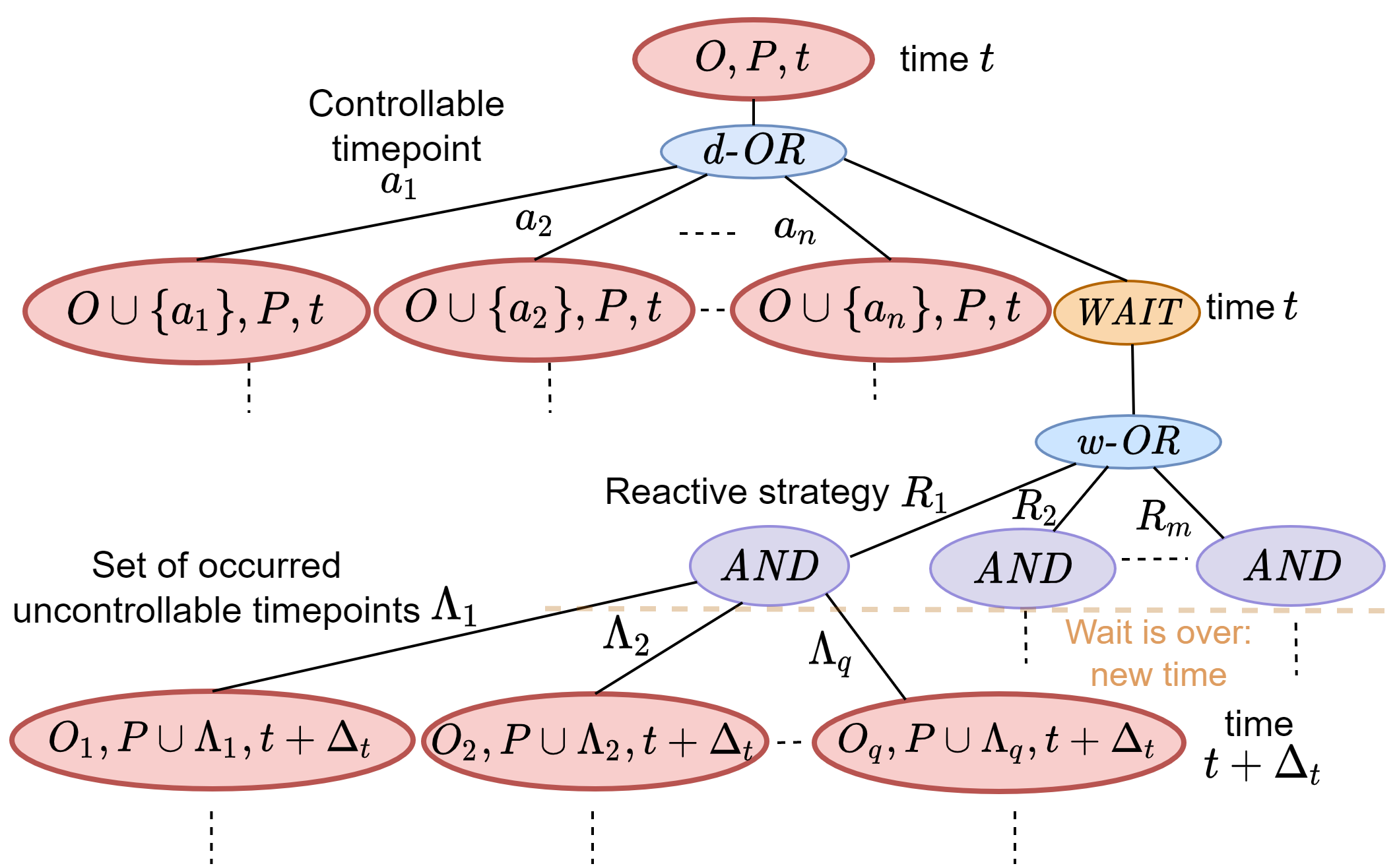
Figure 3: Structure of the search tree. Red nodes are DTNUs; $(O,P,t)$ is a DTNU for which $O$ is the set of controllable timepoints already scheduled, $P$ the set of uncontrollable timepoints that have occurred, and $t$ the time. Each branch $a_{i}$ refers to a controllable timepoint $a_{i}$, $R_{i}$ to a reactive strategy for the wait, and $\Lambda_{i}$ to a combination of uncontrollable timepoints.

Figure 3 illustrates how a sub-problem of $\Gamma$, referred to as $DTNU_{O,P,t}$, is developed, where $O\subset A$ is the set of controllable timepoints that have already been scheduled, $P\subset U$ the set of uncontrollable timepoints which have occurred, and $t$ the time. Moreover, two types of leaf nodes exist in the tree. The first type is a node $DTNU_{A,U,t}$ for which all controllable timepoints $a_{i}\in A$ have been scheduled and all uncontrollable timepoints $u_{i}\in U$ have occurred. The second type is a node $DTNU_{A\setminus A^{\prime},U,t}$ for which all uncontrollable timepoints $u_{i}\in U$ have occurred, but some controllable timepoints $a_{i}\in A^{\prime}$ have not been scheduled. The constraint satisfiability test of the former type of leaf node is straightforward: scheduling times and occurrence time intervals of all timepoints are propagated to constraints. For any timepoint whose occurrence time is only bounded in intervals and not exact, propagation is done in a way which assumes it could have occurred anywhere inside the interval to guarantee soundness. The leaf node’s truth attribute is set to true if all constraints are satisfied, false otherwise. For the latter type, we propagate the occurrence time intervals of all uncontrollable timepoints as well as scheduling times of all scheduled controllable timepoints in the same way, and obtain an updated set of constraint $C^{\prime}$. This leaf node, $DTNU_{A\setminus A^{\prime},U,t}$, is therefore characterized as $\{A^{\prime},\emptyset,C^{\prime},\emptyset\}$ and is a DTN. We add the constraints $a^{\prime}_{i}\geq t,\forall a^{\prime}_{i}\in A^{\prime}$ and use a mixed integer linear programming solver (Cplex (2009)) to solve the DTN. If a solution is found, the time values for each $a_{i}^{\prime}\in A^{\prime}$ are stored and the leaf node’s truth value is set to true. Otherwise, it is set to false. After a truth value is assigned to the leaf node, the truth propagation function defined in § 8.3 in the supplemental is called to logically infer truth value properties for parent nodes. A true value reaching the root node of the tree means a R-TDC strategy has been found. The R-TDC strategy is a subtree of the search tree obtained by selecting recursively from the root, for each d-OR and w-OR nodes, the child with the true attribute, and for each AND node, all children nodes (which are necessarily true). A false attribute reaching the root means there is no existing R-TDC strategy. As a result of the structure of the search tree which explores all possible outcomes of uncontrollable timepoints, and constraint propagation which enforces strict variable domain restrictions after an uncontrollable timepoint is bounded, the algorithm will always return sound strategies. Lastly, the search algorithm explores the tree in a depth-first manner. We describe some simplifications made in the exploration in §8.7 in the supplemental.

4 Tree Search Characteristics

We describe in this section how wait periods are calculated and how constraint propagation is performed. Moreover, we will designate as a conjunct a constraint relationship of the form $v_{i}-v_{j}\in[x,y]$ or $v_{i}\in[x,y]$, where $v_{i},v_{j}$ are timepoints and $x,y,\in\rm I\!R$. We refer to a constraint where several conjuncts are linked by $\lor$ operators as a disjunct.

4.1 Wait Action

When a wait decision of duration $\Delta_{t}$ is taken at time $t$ for a DTNU node, two categories of uncontrollable timepoints are considered to account for all transitional possibilities:

• $Z=\{\zeta_{1},\zeta_{2},...,\zeta_{l}\}$ is a set of timepoints that could either happen during the wait, or afterwards, i.e. the end of the activation time interval for each $\zeta_{i}$ is greater than $t+\Delta_{t}$.

• $H=\{\eta_{1},\eta_{2},...,\eta_{m}\}$ is a set of timepoints that are certain to happen during the wait, i.e. the end of the activation time interval for each $\eta_{i}$ is less than or equal to $t+\Delta_{t}$.

There are $q=2^{l}$ number of different possible combinations (empty set included) $\Upsilon_{1},\Upsilon_{2},...,\Upsilon_{q}$ of elements taken from $Z$. For each combination $\Upsilon_{i}$, the set $\Lambda_{i}=H\cup\Upsilon_{i}$ is created. The union $\bigcup\limits_{i=1}^{q}\Lambda_{i}$ refers to all possible combinations of uncontrollable timepoints which can occur by $t+\Delta_{t}$. In Figure 3, for each AND node, the combination $\Lambda_{i}$ leads to a DTNU sub-problem $DTNU_{O_{i},P\cup\Lambda_{i},t+\Delta_{t}}$ for which the uncontrollable timepoints in $\Lambda_{i}$ are considered to have occurred between $t$ and $t+\Delta_{t}$ in the schedule memory $S$. In addition, any potential controllable timepoint $\phi$ planned to be instantly executed in a reactive wait strategy $R_{i}$ in response to an uncontrollable timepoint $u$ in $\Lambda_{i}$ will also be considered to have been scheduled between $t$ and $t+\Delta_{t}$ in $S$. The only exception is when checking constraint satisfiability for the conjunct $u-\phi\in[0,y]$ which required the reactive execution, for which we assume $\phi$ will be executed by the agent during strategy execution at the same time as $u$, thus the conjunct is considered satisfied.

4.2 Wait Eligibility and Period

The way wait durations are defined holds direct implications on the search space and the capability of the algorithm to find strategies. Longer waits make the search space smaller, but carry the risk of missing key moments where a decision is needed. On the other hand, smaller waits can make the search space too large to explore. We explain when the wait action is eligible, and how its duration is computed.

Eligibility

At least one of these two criteria has to be met for a WAIT node to be added as child of a d-OR node. (1) There is at least one activated uncontrollable timepoint for the parent DTNU node. (2) There is at least one conjunct of the form $v\in[x,y]$, where $v$ is a timepoint, in the constraints of the parent DTNU node. These criteria ensure that the search tree will not develop branches below WAIT nodes when waiting is not relevant, i.e. when a controllable timepoint necessarily needs to be scheduled. It also prevents the tree search from getting stuck in infinite WAIT loop cycles.

Wait Period

We define the wait duration $\Delta_{t}$ at a given d-OR node by examining the updated constraint list $C^{\prime}$ of the parent DTNU and the activation time intervals $B$ of its activated uncontrollable timepoints. Let $t$ be the current time for this DTNU node. Wait duration is defined by comparing $t$ to elements in $C^{\prime}$ and $B$ to look for a minimum positive value defined by the next three rules. Each rule looks at the current partial schedule to identify ’key milestones’ when actions should be taken, allowing to prefer longer waits when nothing is likely to happen before a long time, or shorter waits during critical moments. The purpose of the rules is to make it likely for there to be an existing R-TDC strategy when a DC one exists, while keeping the search space explored by the tree search algorithm as small as possible. (1) For each activated time interval $u\in[x,y]$ in $B$, we select $x-t$ or $y-t$, whichever is smaller and positive, and keep the smallest value $\delta_{1}$ found over all activated time intervals. This rule ensures the algorithm gets the opportunity to take a decision at the very beginning (or end) of a time frame in which an uncontrollable timepoint will occur. (2) For each conjunct $v\in[x,y]$ in $C^{\prime}$, where $v$ is a timepoint, we select $x-t$ or $y-t$, whichever is smaller and positive, and keep the smallest value $\delta_{2}$ found over all conjuncts. This rule gives the algorithm the opportunity to act at the very beginning (or end) of a time frame in which it can satisfy a constraint requiring a timepoint to be in a specific interval. (3) We determine timepoints which need to be scheduled ahead of time by chaining constraints together. Intuitively, when a conjunct $v\in[x,y]$ is in $C^{\prime}$, $v$ has to be scheduled when $t\in[x,y]$ to satisfy this conjunct. However, $v$ may be linked to other timepoints by constraints requiring them to happen before $v$. These timepoints may in turn be linked to yet other timepoints in the same way, and so on. Therefore, waiting until the time constraint window of $v$ may result in the algorithm actually over-waiting and being too late to tackle those constraint dependencies. The third rule consists in chaining backwards to identify potential timepoints starting this chain and potential time intervals in which they need to be scheduled. The following mechanism is used: for each conjunct $v\in[x,y]$ in $C^{\prime}$ found in (2), we apply a recursive chain function to both $(v,x)$ and $(v,y)$. We detail how it is applied to $(v,x)$, the process being the same for $(v,y)$. Conjuncts of the form $v-v^{\prime}\in[x^{\prime},y^{\prime}],x^{\prime}\geq 0$ in $C^{\prime}$ are searched for. For each conjunct found, we add to a list two elements, $(v^{\prime},x-x^{\prime})$ and $(v^{\prime},x-y^{\prime})$. We select $x-x^{\prime}-t$ or $x-y^{\prime}-t$, whichever is smaller and positive, as potential minimum candidate. The chain function is called recursively on each element of the list. We keep the smallest candidate $\delta_{3}$. Figure 9 in the supplemental illustrates an application of this process. Finally, we set $\Delta_{t}=\min(\delta_{1},\delta_{2},\delta_{3})$ as the wait duration. This duration is stored inside the WAIT node.

4.3 Reactive Executions during Waits

Scheduling of a controllable timepoint may be necessary in some situations at the exact same time as when an uncontrollable timepoint occurs to satisfy a constraint. Therefore, different reactive wait strategies are considered and listed as children of a w-OR node after a wait decision, before the start of the wait itself. If at any given DTNU node in the tree there is an activated uncontrollable timepoint $u$ with the potential to occur during the next wait and there is at least one unscheduled controllable timepoint $a$ such that a conjunct of the form $u-a\in[0,y],y\geq 0$ is present in the constraints, a reactive wait strategy is available that will set $a$ to be executed as soon as $u$ occurs during strategy execution.

If there are $s$ controllable timepoints that may be set to be reactively executed, there are $2^{s}$ different reactive wait strategies $R_{i}$, each of which is embedded in an AND child of the w-OR node. Let $\Phi=\{\phi_{1},\phi_{2},...,\phi_{s}\}\subset A$ be the complete set of unscheduled controllable timepoints for which there are conjunct clauses $u-\phi_{i}\in[0,y]$. We denote as $R_{1},R_{2},...,R_{m}$ all possible combinations of elements taken from $\Phi$, including the empty set. The child node $\textit{AND}_{R_{i}}$ of the w-OR node resulting from the combination $R_{i}$ has a reactive wait strategy for which all controllable timepoints in $R_{i}$ will be immediately executed at the moment $u$ occurs during the wait, if it occurs.

4.4 Constraint Propagation

Decisions taken in the tree define when controllable timepoints are scheduled and also bear consequences on the occurrence time of uncontrollable timepoints. We explain here how these decisions are propagated into constraints, as well as the concept of ‘tight bound’.

Let $C^{\prime}$ be the list of updated constraints for a DTNU node $\boldsymbol{\psi}$ for which the parent node is $\boldsymbol{\omega}$. We distinguish two cases. Either $\boldsymbol{\omega}$ is a d-OR node and $\boldsymbol{\psi}$ results from the scheduling of a controllable timepoint $a_{i}$, or $\boldsymbol{\omega}$ is an AND node and $\boldsymbol{\psi}$ results from a wait of $\Delta_{t}$ time units. In the first case, let $t$ be the scheduling time of $a_{i}$. The updated list $C^{\prime}$ is built from the constraints of the parent DTNU of $\boldsymbol{\psi}$ in the tree. If a conjunct contains $a_{i}$ and is of the form $a_{i}\in[x,y]$, this conjunct is replaced with true if $t\in[x,y]$, false otherwise. If the conjunct is of the form $v_{j}-a_{i}\in[x,y]$, we replace the conjunct with $v_{j}\in[t+x,t+y]$. The other possibility is that $\boldsymbol{\psi}$ results from a wait of $\Delta_{t}$ time units at time $t$, with a reactive wait strategy $R$. In this case, the new time is $t+\Delta_{t}$ for $\boldsymbol{\psi}$. As a result of the wait, some uncontrollable timepoints $u_{i}\in\Lambda$ are assumed to have occurred, and some controllable timepoints $a_{i}\in A_{R}$ may be executed reactively during the wait. Let $v_{i}\in\Lambda\cup A_{R}$ be these timepoints occurring during the wait. The occurrence time of these timepoints is assumed to be in [$t$, $t+\Delta_{t}$]. For uncontrollable timepoints $u_{i}^{\prime}\in\Lambda^{\prime}\subset\Lambda$ for which the activation time ends at $t+\Delta_{t_{i}}^{\prime}<t+\Delta_{t}$, and potential controllable timepoints $a_{i}^{\prime}$ instantly reacting to these uncontrollable timepoints, the occurrence time is further reduced and considered to be in $[t,t+\Delta_{t_{i}}^{\prime}]$.

We define a concept of tight bound to update constraints which restricts time intervals in order to account for all possible values $v_{i}$ can take between $t$ and $t+\Delta_{t}$. For all conjuncts $v_{j}-v_{i}\in[x,y]$, we replace the conjunct with $v_{j}\in[t+\Delta_{t}+x,t+y]$. Intuitively, this means that since $v_{i}$ can happen at the latest at $t+\Delta_{t}$, $v_{j}$ can not be allowed to happen before $t+\Delta_{t}+x$. Likewise, since $v_{i}$ can happen at the earliest at $t$, $v_{j}$ can not be allowed to happen after $t+y$. Finally, if $t+\Delta_{t}+x>t+y$, the conjunct is replaced with false . Also, the process can be applied recursively in the event that $v_{j}$ is also a timepoint that occurred during the wait, in which case the conjunct would be replaced by true or false. In any case, any conjunct obtained of the form $a_{j}\in[x^{\prime},y^{\prime}]$ is replaced with false if $t+\Delta_{t}>y^{\prime}$. Finally, if all conjuncts inside a disjunct are set to false by this process, the constraint is violated and the DTNU is no longer satisfiable.

5 Learning-based Heuristic

We explain here how our learning model provides tree search guidance. Our MPNN architecture stems from Gilmer et al. (2017). It uses message passing rules enabling it to process graph-structured inputs. This architecture was originally designed for node classification in quantum chemistry and achieved state-of-the-art results on a molecular property prediction benchmark. Here, we define a way of converting DTNUs into graph data. Then, we process the graph data with a fixed MPNN architecture and use the output to guide the tree search.

Let $\Gamma=\{A,U,C,L\}$ be a DTNU. We explain how we turn $\Gamma$ into a graph $\mathcal{G}=(\mathcal{K},\mathcal{E})$. First, we convert all time values from absolute to relative by setting the current time for $\Gamma$ to $t=0$. We search all converted time intervals $[x_{i},y_{i}]$ in $C$ and $L$ for the highest interval bound value $d_{max}$, i.e. the farthest point in time. We normalize every time value in $C$ and $L$ by dividing them by $d_{max}$, yielding values between $0$ and $1$. Next, we convert each controllable timepoint $a\in A$ and uncontrollable timepoint $u\in U$ into graph nodes with corresponding controllable or uncontrollable node features. Time constraints in $C$ and contingency links in $L$ are expressed as edges between nodes with $10$ different edge distance classes ($0:[0,0.1)$, $1:[0.1,0.2)$, …, $9:[0.9,1]$). We also use additional edge features to account for edge types (constraint, disjunction, contingency link, direction sign for lower and upper bounds). Moreover, intermediary nodes are used with a distinct node feature in order to map possible disjunctions in constraints and contingency links. We add a WAIT node with a distinct node feature which implicitly designates the act of waiting a period of time. Figure 10 in the supplemental shows an example of DTNU graph conversion.

The graph conversion of DTNU $\gamma$ contains three elements: the matrix of all node features $X_{\kappa}$, the adjacency matrix of the graph $X_{\epsilon}$ and the matrix of all edge features $X_{\rho}$. These features are processed by a fixed number of consecutive message passing layers from Gilmer et al. (2017) which make the MPNN. Each layer takes an input graph, consists of a phase during which messages are passed between nodes, and returns the same graph with new node features. Edge features remain the same. The overall process for a layer is as follows. For each node $\kappa_{i}$ in the input graph, a message passing phase creates new features for $\kappa_{i}$ from current features of neighboring nodes and edges. In detail, for each neighbor node $\kappa_{j}$, a small neural network (termed multi-layer perceptron, or MLP) takes as input the features of the edge connecting $\kappa_{i}$ and $\kappa_{j}$ and returns a matrix which is then multiplied by the features of $\kappa_{j}$ to obtain a feature vector. The sum of these vectors for the entire neighborhood defines the new features for $\kappa_{i}$. The output of the message passing layer consists of the graph updated with the new node features. In each message passing layer, the same MLP is used to process every node, so it can be applied to input graphs of any size, i.e. the MPNN architecture can take as input DTNUs of any size. Moreover, each message passing layer uses a different MLP and can thus be trained to learn a different message passing scheme. Algorithm 3 in the supplemental explains the workings of message passing.

Let $f$ be the function for our MPNN and $\theta$ its parameters. Function $f$ stacks $5$ message passing layers coupled with the $\mathrm{ReLU}(\cdot)=\max(0,\cdot)$ piece-wise activation function (Glorot, Bordes, and Bengio (2011)) after each layer, except the last one. The first 4 layers have 32 abstract features per node, the last layer has 1 abstract feature per node. Each layer uses a trainable two-layer multi-layer perceptron (with 128 neurons in the hidden layer) for the message passing. Moreover, we add skip connections (He et al. (2016)) to link each layer to the previous one. The sigmoid function $\sigma(\cdot)=\frac{1}{1+\exp(-\cdot)}$ is used after the last layer to obtain a list of probabilities $\pi$ over all nodes in $\mathcal{G}$ : $f_{\theta}(X_{\kappa},X_{\epsilon},X_{\rho})=\pi$. The probability of each node $\kappa$ in $\pi$ corresponds to the likelihood of transitioning into a R-TDC DTNU from the original DTNU $\Gamma$ by taking the action corresponding to $\kappa$. If $\kappa$ represents a controllable timepoint $a$ in $\Gamma$, its corresponding probability in $\pi$ is the likelihood of the sub-DTNU resulting from the scheduling of $a$ being R-TDC. If $\kappa$ represents a WAIT decision, its probability refers to the likelihood of the WAIT node having a true attribute, We call these two types of nodes active nodes. Otherwise, if $\kappa$ is another type of node, its probability is not relevant to the problem and ignored. Our MPNN is trained on DTNUs generated and solved in § 8.8 in the supplemental only on active nodes by minimizing the binary cross-entropy loss:

$$\frac{1}{m}\sum\limits_{i=1}^{m}\sum\limits_{j=1}^{q}-Y_{ij}\log(f_{\theta}(X_{i})_{j})-(1-Y_{ij})\log(1-f_{\theta}(X_{i})_{j})$$

Here $X_{i}=(X_{i_{\kappa}},X_{i_{\epsilon}},X_{i_{\rho}})$ is DTNU number $i$ among a training set of $m$ examples, $Y_{ij}$ is the R-TDC controllability (1 or 0) of active node number $j$ for DTNU number $i$. During training, we use batch normalization after each message passing layer. We add a dropout regularization layer with a keep rate $0.9$ before the output layer to reduce overfitting. Training is done with the adagrad optimizer from Duchi, Hazan, and Singer (2011) and an initial learning rate $10^{-4}$ on a dataset comprised of $30K$ instances generated as described in § 8.8 in the supplemental. We split the data into a training set comprised of $25K$ instances and a cross-validation set comprised of $5K$ instances on which we achieve $84\%$ accuracy. Lastly, the MPNN heuristic is used as follows in the tree search. Once a d-OR node is reached, its parent DTNU node is converted into a graph and the MPNN is called upon the corresponding graph elements $X_{\kappa},X_{\epsilon},X_{\rho}$. Active nodes in output probabilities $\pi$ are then ordered by highest values first, and the search visits the corresponding children nodes in the suggested order, preferring children with higher likelihood of being R-TDC first.

6 Experiments

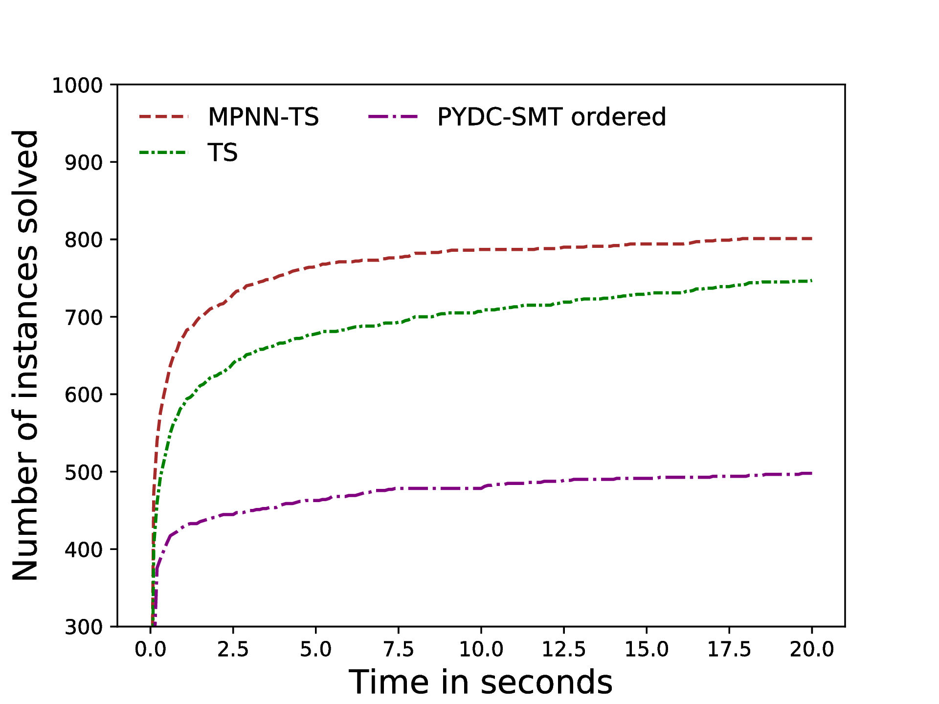
Figure 4: Experiments on (Cimatti, Micheli, and Roveri 2016)’s benchmark. The X-axis shows the allocated time (s) and the Y-axis the number of instances each solver can solve within the corresponding allocated time. Timeout is set to 20 seconds per instance.

We evaluate the efficiency of the tree search and the effect of the MPNN’s guidance. We also compare them to the state-of-the-art DC solver, PYDC-SMT-ordered, from Cimatti, Micheli, and Roveri (2016) on a same computer. The tree search algorithm, trained MPNN and benchmarks are available here. We use a laptop with the following specifications for experiments: $9^{th}$ gen. Intel Core i7, 16GB RAM and nvidia GTX 1660 Ti. R-TDC is a subset of DC and TDC: non-R-TDC controllability does not imply non-DC controllability. A R-TDC solver can thus be expected to offer better performance than a DC one while potentially being unable to find a strategy when a DC algorithm would. In this section, we refer to the tree search algorithm as TS and the tree search algorithm guided by the trained MPNN up to the $15^{th}$ (respectively $X^{th}$) d-OR node depth-wise in the tree as MPNN-TS (respectively MPNN-TS-X).

First, we use the benchmark from Cimatti, Micheli, and Roveri (2016) from which we remove DTNs and STNs. We compare TS, MPNN-TS and PYDC-SMT on the resulting benchmark which is comprised of $290$ DTNUs and $1042$ STNUs. Here, Limiting maximum depth use of the MPNN to $15$ offers a good trade off between guidance gain and cost of calling the MPNN. Results are given in Figure 4. We observe TS solves roughly $50\%$ more problem instances than PYDC-SMT within the allocated time ($20$ seconds). In addition, TS solves $56\%$ of all instances while the remaining ones time out. Among solved instances, a strategy is found for $89\%$ and the remaining $11\%$ are proved non-R-TDC. On the other hand, PYDC-SMT solves $37\%$ of all instances. A strategy is found for $85\%$ of PYDC-SMT’s solved instances, the remaining $15\%$ are proved non-DC. Finally, out of all instances PYDC-SMT solves, TS solves $97\%$ with the same conclusion, i.e. R-TDC when DC and non-R-TDC when non-DC, highlighting the significant completeness retained by R-TDC. The use of the MPNN leads to an additional $+6\%$ problems solved. We argue this small increase is essentially due to the fact that most problems solved in the benchmark are small-sized problems with few timepoints which are solved quickly. Despite this fact, the MPNN still provides performance boost on a benchmark generated with another DTNU generator, suggesting the bias introduced by our DTNU generator remains limited and the MPNN is able to generalize to DTNUs created with a different approach.

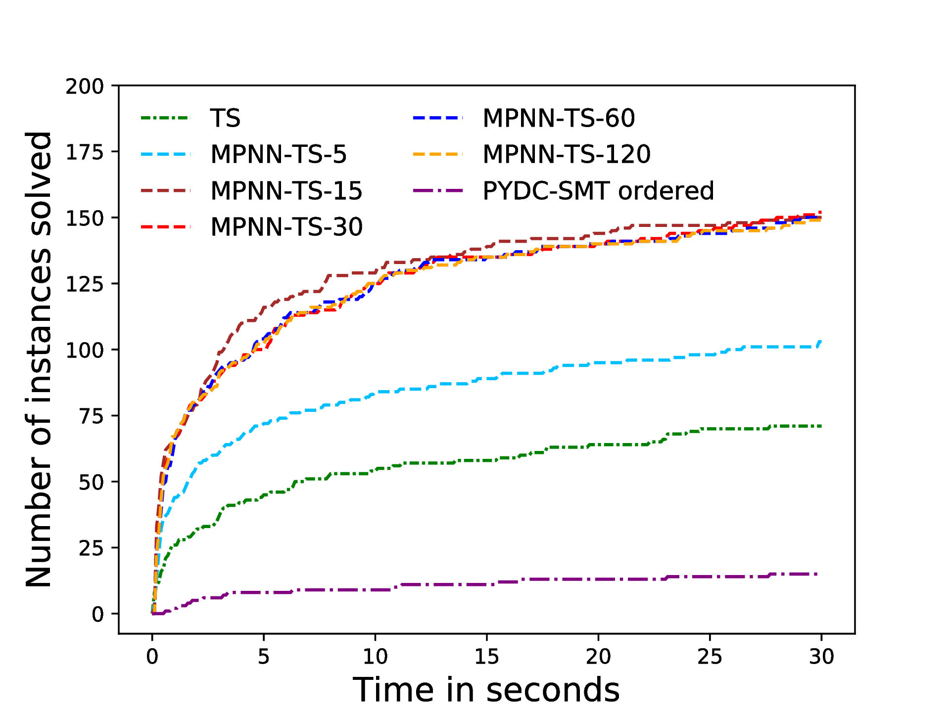
Figure 5: Experiments on benchmark $\boldsymbol{B_{1}}$. Axes are as in Figure 4. Timeout is set to 30 seconds per instance.

For further evaluation of the MPNN, we create new benchmarks with the DTNU generator from § 8.8 (supplemental) with varying number of timepoints. These benchmarks have fewer quick to solve DTNUs and harder ones instead. Each benchmark contains 500 random DTNUs which have $1$ to $3$ uncontrollable timepoints. Moreover, each DTNU has 10 to 20 controllable timepoints in the $1^{st}$ benchmark $B_{1}$, 20 to 25 in the $2^{nd}$ benchmark $B_{2}$ and 25 to 30 in the last benchmark $B_{3}$. Each disjunct in the constraints of any DTNU contains up to 5 conjuncts. Experiments on $B_{1}$, $B_{2}$ and $B_{3}$ are respectively shown in Figure 5, 7(c) (in the supplemental) and 6. We note that for all three benchmarks no solver ever proves non-R-TDC or non-DC controllability before timing out due to the larger size of these problems.

PYDC-SMT performs poorly on $B_{1}$ and cannot solve any instance on $B_{2}$ and $B_{3}$. TS underperforms on $B_{2}$ and only solves 2 instances on $B_{3}$. However, we see a significantly higher gain from the use of the MPNN, varying with the maximum depth use. At best depth use, the gain is $+91\%$ instances solved for $B_{1}$, $+980\%$ for $B_{2}$ and $+1150\%$ for $B_{3}$. The more timepoints instances have, the more worthwhile MPNN guidance appears to be. Indeed, the optimal maximum depth use of the MPNN in the tree increases with the problem size: $15$ for $B_{1}$, $60$ for $B_{2}$ and $120$ for $B_{3}$. We argue this is due to the fact that more timepoints results in a wider search tree overall, including in deeper sections where MPNN use was not necessarily worth its cost for smaller problems. Furthermore, the MPNN is trained on randomly generated DTNUs which have 10 to 20 controllable timepoints. The promising gains shown by experiments on $B_{2}$ and $B_{3}$ suggest generalization of the MPNN to bigger problems than it is trained on.

The proposed tree search approach presents a good trade off between search completeness and effectiveness: almost all examples solved by PYDC-SMT in the benchmark of Cimatti, Micheli, and Roveri (2016) are solved with the same conclusion, and many more which could not be solved are. Moreover, the R-TDC approach scales up better to problems with more timepoints, and the tree structure allows the use of learning-based heuristics. Although these heuristics are not key to solving problems of big scales, our experiments suggest they can still provide a high increase in efficiency.

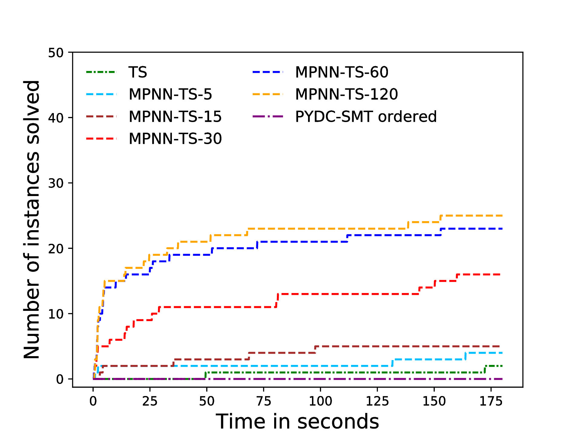
Figure 6: Experiments on benchmark $\boldsymbol{B_{3}}$. Axes are as in Figure 4. Timeout is set to 180 seconds.

7 Conclusion

We introduced new semantics for reactive scheduling: Time-based Dynamic Controllability (TDC) and a restricted subset of TDC, R-TDC. We presented a tree search approach for solving Disjunctive Temporal Networks with Uncertainty (DTNU) in R-TDC. Strategies are built by discretizing time and exploring different decisions which can be taken at different key points, as well as anticipating how uncontrollable timepoints can unfold. We showed experimentally that R-TDC retains significant completeness, and enables the tree search approach to process DTNUs more efficiently than the state-of-the-art Dynamic Controllability (DC) solver does in DC. Lastly, we created MPNN-TS, a solver which combines the tree search with a heuristic function based on a graph neural network for guidance. The graph neural network enables steady improvements of the tree search on harder DTNU problems, notably on DTNUs of bigger size than those used for training the graph neural network.

8 Technical Appendix

8.1 Summary of Experiments on all Benchmarks

The plot for benchmark $B_{2}$, not provided in the paper, is given in Figure 7(c).

(a) Experiments on (Cimatti, Micheli, and Roveri 2016)’s benchmark. The X-axis represents the allocated time in seconds and the Y-axis the total number of instances that each solver can solve within the corresponding allocated time. Timeout is set to 20 seconds per instance.

(b) Experiments on benchmark $B_{1}$. Axes are the same as in figure 7(a). Timeout is set to 30 seconds per instance.

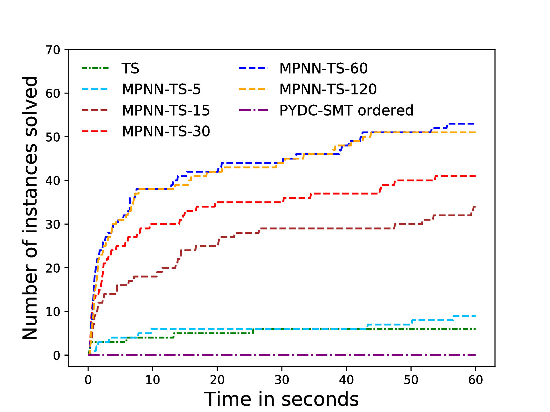
(c) Experiments on benchmark $B_{2}$. Axes are the same as in figure 7(a). Timeout is set to 60 seconds per instance.

(d) Experiments on benchmark $B_{3}$. Axes are the same as in figure 7(a). Timeout is set to 180 seconds per instance.

Figure 7: Summary of experiments on benchmarks

8.2 Simplified Example

Figure 8 is a detailed R-TDC strategy of the example DTNU from (Cimatti, Micheli, and Roveri 2016).

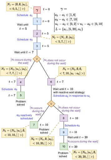
Figure 8: Detailed R-TDC strategy of a DTNU $\Gamma$. The red square $\gamma$ is the original DTNU. Other squares are sub-DTNUs, except the $\lor$ signs which list transitional possibilities. Nodes $N_{i}$ represent the R-TDC strategy nodes as explained in the definition section.

8.3 Truth Value Propagation

We describe how truth attributes of nodes are related to each other. The truth attribute of a tree node represents its R-TDC controllability, and the relationships shared between nodes make it possible to define sound strategies. When a leaf node is assigned a truth attribute $\beta$, the tree search is momentarily stopped and $\beta$ is propagated onto upper parent nodes. To this end, a parent node $\boldsymbol{\omega}$ is selected recursively and we distinguish the following cases:

• The parent $\boldsymbol{\omega}$ is a DTNU or WAIT node: $\boldsymbol{\omega}$ is assigned $\beta$.

• The parent $\boldsymbol{\omega}$ is a d-OR or w-OR node: If $\beta=true$, then $\boldsymbol{\omega}$ is assigned true . If $\beta=false$ and all children nodes of $\boldsymbol{\omega}$ have false attributes, $\boldsymbol{\omega}$ is assigned false . Otherwise, the propagation stops.

• The parent $\boldsymbol{\omega}$ is an AND node: If $\beta=false$, then $\boldsymbol{\omega}$ is assigned false . If $\beta=true$ and all children nodes of $\boldsymbol{\omega}$ have true attributes, $\boldsymbol{\omega}$ is assigned true . Otherwise, the propagation stops.

After the propagation finishes, the tree search algorithm resumes where it was stopped. Algorithm 1 describes this process.

Algorithm 1 Truth Value Propagation

1:function propagateTruth(TreeNode $\psi$)

2:     $\omega\leftarrow$ parent($\psi$) $\triangleright$ ${}^{1}*$

3:     if $\omega=null$ then

4:         return      

5:     if isDTNU($\omega$) or isWAIT($\omega)$ then $\triangleright$ ${}^{2}*$

6:         $\omega.truth\leftarrow\psi.truth$

7:         propagateTruth($\omega$)

8:     else if isOR($\omega$) then $\triangleright$ ${}^{3}*$

9:         if $\psi.truth=True$ then

10:              $\omega.truth\leftarrow True$

11:              propagateTruth($\omega$)

12:         else

13:              if $\forall\sigma_{i},\sigma_{i}.truth=False$ then $\triangleright$ ${}^{4}*$

14:                  $\omega.truth\leftarrow False$

15:                  propagateTruth($\omega$)                        

16:     else if isAND($\omega$) then $\triangleright$ ${}^{5}*$

17:         if $\psi.truth=False$ then

18:              $\omega.truth\leftarrow False$

19:              propagateTruth($\omega$)

20:         else

21:              if $\forall\sigma_{i},\sigma_{i}.truth=True$ then $\triangleright$ ${}^{4}*$

22:                  $\omega.truth\leftarrow True$

23:                  propagateTruth($\omega$)                             

$*$ parent($x$): Returns the parent node of $x$, $null$ if none.
$*$ isDTNU($x$): Returns True if $x$ is a DTNU node, False otherwise; isWait($x$): Returns True if $x$ is a WAIT node, False otherwise.
$*$ isOR($x$): Returns True if $x$ is an d-OR or w-OR node, False otherwise.
$*$ $\sigma_{i}$: Child number $i$ of $\omega$. For a d-OR or w-OR node, in the case where $\psi$ is false but not all other children of $\omega$ are false the propagation stops. Likewise, for an AND node and in the case where $\psi$ is true but not all other children of $\omega$ are true , the propagation stops.
$*$ isAnd($x$): Returns True if $x$ is an AND node, False otherwise.

8.4 Tree Search Algorithm

We give the simplified pseudocode for the tree search in Algorithm 2.

Algorithm 2 Tree Search

1:function explore(TreeNode $\psi$)

2:     if $parent(\psi).truth\neq unknown$ then

3:         return      

4:     if isDTNU($\psi$) then

5:         updateConstraints($\psi$) $\triangleright$ ${}^{6}*$

6:         if IsLeaf($\psi$) then $\triangleright$ ${}^{7}*$

7:              propagateTruth($\psi$)

8:              return          

9:         Create d-OR child $\psi^{\prime}$

10:         explore($\psi^{\prime}$)      

11:     if isOR($\psi$) then

12:         Create list of all children $\Psi^{\prime}$ $\triangleright$ ${}^{8}*$

13:         for $\psi^{\prime}\in\Psi^{\prime}$ do

14:              explore($\psi^{\prime}$)               

15:     if isAND($\psi$) then

16:         Create list of all children $\Psi^{\prime}$ $\triangleright$ ${}^{9}*$

17:         for $\psi^{\prime}\in\Psi^{\prime}$ do

18:              explore($\psi^{\prime}$)               

19:     if isWAIT($\psi$) then

20:         create w-OR child $\psi^{\prime}$

21:         explore ($\psi^{\prime}$)      

22:function main(DTNU $\gamma$)

23:     explore($\gamma$)

24:     if $\gamma.truth=True$ then

25:         return $True$

26:     else

27:         return $False$      

$*$ updateConstraints($x$): Updates the constraints of DTNU node $x$.

$*$ isLeaf($x$): Sets the truth value of $x$ to true and returns true if all constraints are satisfied. Sets the truth value to false and returns true if a constraint is violated. If no truth value can be inferred at this stage with the updated constraints, a second check is run to determine if all uncontrollable timepoints have occurred. If so, the corresponding DTN is solved, the truth value of $x$ is updated accordingly, and the function returns true . Otherwise, no logical outcome can be inferred for the current state of the constraints because there remains at least one uncontrollable timepoint and this function returns false .

$*$ If this is a d-OR node, the list $\Psi^{\prime}$ contains all the children DTNU nodes resulting from either the decision of scheduling a controllable timepoint, or the WAIT node resulting from a wait if available. If this is a w-OR node, $\Psi^{\prime}$ contains all AND${}_{R_{j}}$ nodes, each of which possess a reactive wait strategy $R_{j}$

$*$ Here, the list $\Psi^{\prime}$ contains all DTNUs resulting from all possible combinations $\Lambda_{1},\Lambda_{2},...,\Lambda_{q}$ of uncontrollable timepoints which have the potential to occur during the current wait.

8.5 Soundness of Strategies

We remind the reader that if a true attribute reaches the root node of the search tree of a DTNU, a R-TDC strategy has been found and search terminates. The R-TDC strategy is a subtree of the search tree obtained by selecting recursively from the root, for each d-OR and w-OR nodes, the child with the true attribute, and for each AND node, all children nodes (which are necessarily true). Hence, all nodes, including leaf nodes, of this sub-tree have a true attribute. Rules of constraint propagation are as defined in § 4.4: when a controllable timepoint is scheduled at a d-OR node, its exact execution time is incorporated to the partial schedule; when an uncontrollable timepoint is assumed to have occurred from $t$ to $t+\Delta_{t}$ during a wait, it is considered in the partial schedule that this timepoint has occurred at all possible times in the interval $[t,t+\Delta_{t}]$ through the concept of tight bound. Furthermore, the structure of the sub-tree guarantees coverage of the entire time horizon and includes all possible outcomes of uncontrollable timepoints given wait durations.

Lemma 8.1.

A R-TDC strategy found by the algorithm is sound and guarantees satisfiability of constraints.

Proof.

Let us assume there is a controllable timepoint $a$ in one of the leaf nodes with a schedule $t$ that causes unsatisfiability of constraints. This would cause the leaf node to have a false attribute as a result of constraint propagation, which is contradictory. Let us now suppose there is an uncontrollable timepoint $u$ in one of the leaf nodes which is assumed to have occurred between $t$ and $t+\Delta_{t}$, and for which an occurrence time at $t^{\prime}\in[t,t+\Delta_{t}]$ causes constraints of the leaf node to be violated. This also implies that propagating the interval $u\in[t,t+\Delta_{t}]$ in the constraints through the concept of tight bound results in the leaf node having a false attribute since there is a time value $t^{\prime}\in[t,t+\Delta_{t}]$ which violates constraints. This is contradictory as well.

∎

8.6 Wait Period

Figure 9 gives an example of the third rule used to compute a wait duration.

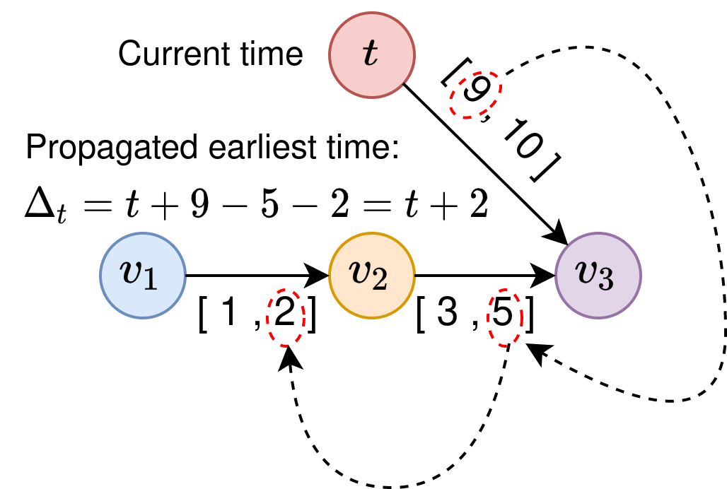
Figure 9: Application of the $3^{rd}$ rule to determine a wait duration. Current time is $t$. Variables $v_{1}$, $v_{2}$ and $v_{3}$ are timepoints. Here, $v_{2}$ is constrained to be scheduled in the time interval $[1,2]$ after $v_{1}$, $v_{3}$ in $[3,5]$ after $v_{2}$ as well as in $[t+9,t+10]$. The rule suggests not to wait longer than $2$ units of time at $t$: scheduling $v_{1}$ at $t+2$, followed by scheduling $v_{2}$ at $t+4$ opens a window of opportunity for $v_{3}$ to be scheduled at $t+9$.

8.7 Optimization Rules

The following rules are added to make branch cuts.

Constraint Check.

When a DTNU node is explored and the updated list of constraints $C^{\prime}$ is built according to §4.4, if a disjunct is found to be false , $C^{\prime}$ will no longer be satisfiable. All the subtree which can be developed from the DTNU will only have leaf nodes for which this is the case as well. The search algorithm will not develop this subtree.

Symmetrical subtrees.

Some situations can lead to the development of the exact same subtrees. A trivial example, for a given DTNU node at a time $t$, is the order in which a given combination of controllable timepoints $a_{1},a_{2},...,a_{k}$ is taken before taking a wait decision. Regardless of what order these timepoints are explored in the tree before moving to a WAIT node, they will be considered scheduled at time $t$. When taking a wait decision, it is thus checked that all preceding controllable timepoints scheduled before the previous wait are a combination of timepoints that has not been tested yet.

Truth Checks.

Before exploring a new node for which the truth attribute is set to unknown, the truth attribute of the parent node is also checked. The node is only developed if the parent node’s truth attribute is set to unknown. In this manner, when children of a tree node are being explored (depth-first) and the exploration of a child node leads to the assignment of a truth value to the tree node, the remaining unexplored children can be left unexplored.

8.8 Self-Supervised Learning

We leverage a learning-based heuristic to guide the tree search. A key component in learning-based methods is the annotated training data. We generate such data in automatic manner by using a DTNU generator to create random DTNU problems and solving them with a modified version of the tree search. We store results and use them for training the MPNN. We detail here our data generation strategy.

We create DTNUs with a number of controllable timepoints ranging from 10 to 20 and uncontrollable timepoints ranging from 1 to 3. The generation process is the following. For interval bounds of constraint conjuncts or contingency links, we randomly generate real numbers within $[0,100]$. We restrict the number of conjuncts inside a disjunct to 5 at most. A random number $n_{1}\in[10,20]$ of controllable timepoints and $n_{2}\in[1,3]$ of uncontrollable timepoints are selected. Each uncontrollable timepoint is randomly linked to a different controllable timepoint with a contingency link. Next, we iterate over the list of timepoints, and for each timepoint $v_{i}$ not appearing in constraints or contingency links, we add in the constraints a disjunct for which at least one conjunct constrains $v_{i}$. The type of conjunct is selected randomly from either a distance conjunct $v_{i}-v_{j}\in[x,y]$ or a bounded conjunct $v_{i}\in[x,y]$. On the other hand, if $v_{i}$ was already present in the constraints or contingency links, we add a disjunct constraining $v_{i}$ with only a $20\%$ probability.

In order to solve these DTNUs, we modify the tree search as follows. For a DTNU $\Gamma$, the first d-OR child node is developed as well as its children $\psi_{1},\psi_{2},...,\psi_{n}\in\Psi$. The modified tree search explores each $\psi_{i}$ multiple times ($\nu$ times at most), each time with a timeout of $\tau$ seconds. We set $\nu=25$ and $\tau=3$. For each exploration of $\psi_{i}$, children nodes of any d-OR node encountered in the corresponding subtree are explored randomly each time. If $\psi_{i}$ is proved to be either R-TDC or non-R-TDC during an exploration, the next explorations of the same child $\psi_{i}$ are called off and the truth attribute $\beta_{i}$ of $\psi_{i}$ is updated accordingly. The active node number $k$, corresponding to the decision leading to $\psi_{i}$ from DTNU $\Gamma$’s d-OR node, is updated with the same value, i.e. $Y_{k}=\beta_{i}$ ($1$ for true, $0$ for false). If every exploration times out, $\psi_{i}$ is assumed non-R-TDC and $Y_{k}$ is set to false. Once each $\psi_{i}$ has been explored, the pair $\langle G(\Gamma),(Y_{1},Y_{2},...,Y_{n})\rangle$ is stored in the training set, where $G(\Gamma)$ is the graph conversion of $\Gamma$ described in §5. Data related to solved sub-DTNUs of $\Gamma$ are not stored in the training set as it was found to cause bias issues and overall decrease generalization in MPNN predictions.

The assumption of non-R-TDC controllability for children nodes for which all explorations time out is acceptable in the sense that the heuristic used is not admissible and does not need to be. The output of the MPNN is a probability for each child node of the d-OR node, creating a preferential order of visit by highest probabilities first. Even in the event the suggested order first recommends visiting children nodes which will be found to be non-R-TDC, the algorithm will continue to explore the remaining children nodes until one is found to be R-TDC. Nevertheless, such a scenario rarely occurs in our experiments as the trained MPNN gives higher probabilities for children nodes for which explorations would tend to find a R-TDC strategy before timeout, and lower probabilities for ones where explorations would tend to result in a timeout.

8.9 Message Passing Layer and DTNU to Graph Conversion

We use message passing layers that take as input a graph where nodes and edges possess features and return the graph with new node features. We detail pseudocode of a message passing layer applied to a graph $\mathcal{G=(K,E)}$ in Algorithm 3. Additionally, we provide in Figure 10 an example of a DTNU converted into a graph.

Algorithm 3 Message Passing Layer

1:function MsgPass(Graph $\langle\mathcal{(K,E)},(H_{\kappa},X_{\epsilon},X_{\rho})\rangle$) $\triangleright$ ${}^{10}*$

2:     $H_{\kappa}^{\prime}(\cdot,\cdot)\leftarrow 0$ // Initialize new node features matrix

3:     for all $\kappa_{i}\in\mathcal{K}$ do

4:         $h_{i}^{\prime}\leftarrow 0$ // Initialize new features for $\kappa_{i}$

5:         for all $\kappa_{j}\in\mathcal{K}$ do

6:              if $X_{\epsilon}(\kappa_{i},\kappa_{j})=1$ then

7:                  $\alpha\leftarrow X_{\rho}(\kappa_{i},\kappa_{j})$

8:                  $h\leftarrow H_{\kappa}(\kappa_{j},\cdot)$

9:                  $h_{i}^{\prime}\leftarrow h_{i}^{\prime}+MLP(\alpha)h$ $\triangleright$ ${}^{11}*$                        

10:         $H_{\kappa}^{\prime}(\kappa_{i},\cdot)\leftarrow h_{i}^{\prime}$ // Assign new features for $\kappa_{i}$      

11:     return $\langle\mathcal{(K,E)},(H_{\kappa}^{\prime},X_{\epsilon},X_{\rho})\rangle$

$*$ $H_{\kappa}(\kappa_{i},\cdot)$ returns a vector of current features for node $\kappa_{i}$; $X_{\epsilon}(\kappa_{i},\kappa_{j})$ returns $1$ if $(\kappa_{i},\kappa_{j})\in\mathcal{E}$, $0$ otherwise; $X_{\rho}(\kappa_{i},\kappa_{j})$ returns a vector of current features for edge $(\kappa_{i},\kappa_{j})$.
$*$ MLP represents a multi-layer perceptron mapping input edge features to a matrix of dimension num-output-node-features x num-input-node-features. Moreover, $h$ is of dimension num-input-node-features x $1$. The matrix multiplication therefore results in a vector of size num-output-node-features.

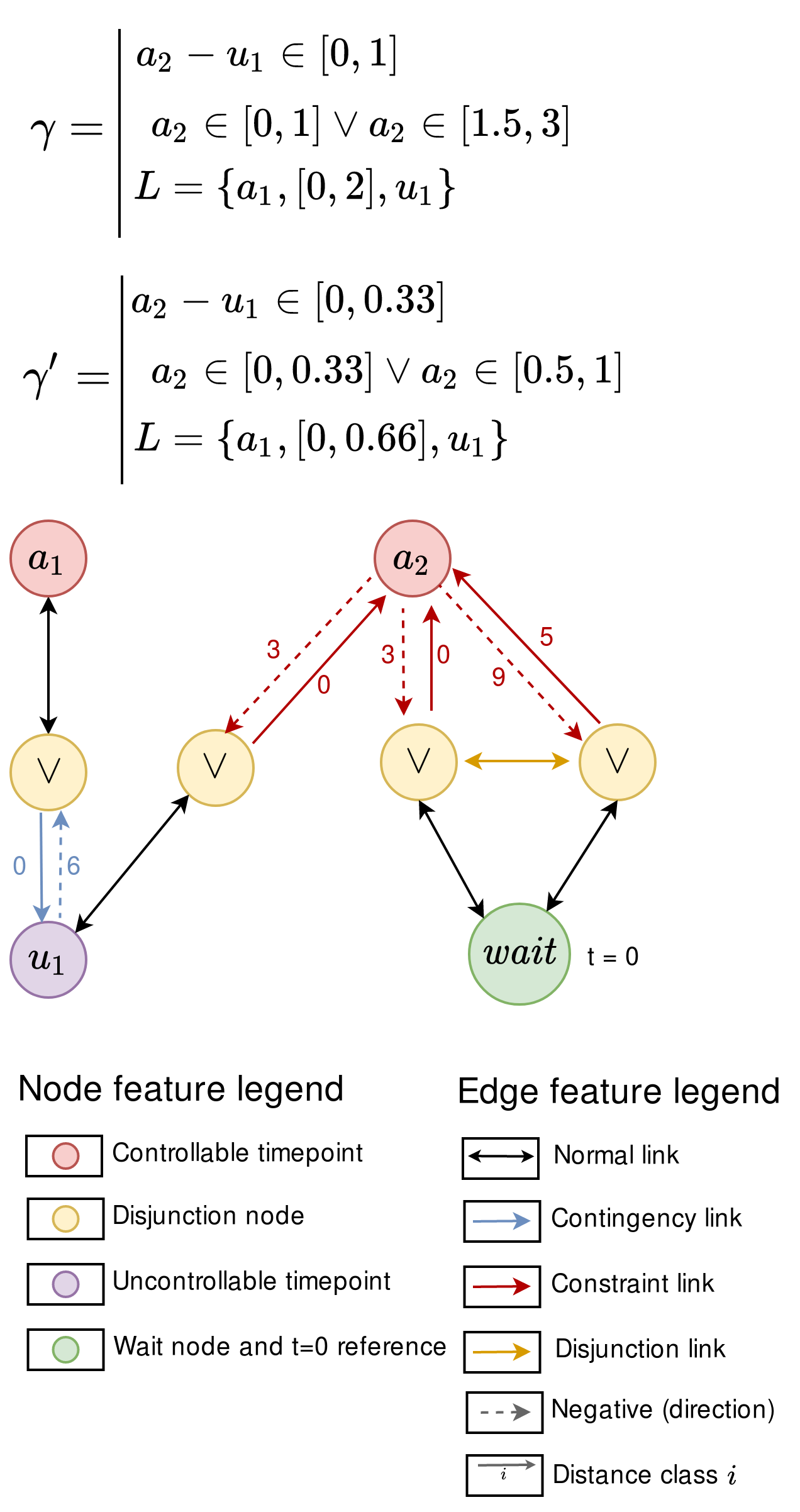
Figure 10: Conversion of a DTNU $\gamma$ into a graph. $\gamma^{\prime}$ is the normalized DTNU. Edge distances are expressed as distance classes. To distinguish between lower and upper bounds in intervals, we introduce an additional negative directional sign feature.

8.10 Architecture Comparison

We study the impact of the design choices of the MPNN architecture on performance. To this end we compare different architectures of MPNN by varying depth and width (number of abstract node features per layer) and train them on the training set created in §8.8. We also assess the added value of residual skip connections to preceding layers. We create a benchmark of 400 DTNU instances, each of which has 20 to 25 controllable timepoints and up to 3 uncontrollable timepoints. We solve them using the tree search guided by each of these MPNN architectures. We limit the use of the MPNN architectures to a maximal depth of $50$ (d-OR node-wise). Results are shown in Figure 11. We note the smallest network is too small to learn efficiently and performs poorly. Three-layer networks perform better. Wider networks perform slightly better for the same depth, black network 32 vs. green network 16. Overall, medium-depth networks of 5 layers work best. Residual connections lead to slight but steady gains. Interestingly, deeper networks (8+ layers) display lower scores compared to more shallower variants (5 layers), suggesting depth performance saturation. The quantity of training data can however be a limiting factor: we assume the optimal architecture to be actually deeper.

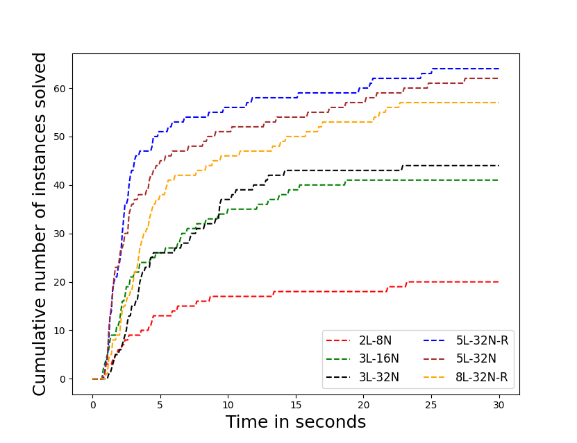
Figure 11: Comparison of different MPNN architectures. Notation XL-YN refers to an MPNN with X layers and Y abstract node features per layer. The ”-R” tag refers to the presence of residual layers. Timeout is set to 30 seconds per DTNU instance.

References

- Akmal et al. (2019) Akmal, S.; Ammons, S.; Li, H.; and Boerkoel Jr, J. C. 2019. Quantifying degrees of controllability in temporal networks with uncertainty. In Proceedings of the International Conference on Automated Planning and Scheduling, volume 29, 22–30.
- Battaglia et al. (2016) Battaglia, P.; Pascanu, R.; Lai, M.; Rezende, D. J.; et al. 2016. Interaction networks for learning about objects, relations and physics. In Advances in neural information processing systems, 4502–4510.
- Bhargava et al. (2018) Bhargava, N.; Muise, C.; Stegun, T. V.; and Williams, B. C. 2018. Managing Communication Costs under Temporal Uncertainty. In Proceedings of the Twenty-Seventh International Joint Conference on Artificial Intelligence, 84–90.
- Bhargava and Williams (2019a) Bhargava, N.; and Williams, B. C. 2019a. Complexity Bounds for the Controllability of Temporal Networks with Conditions, Disjunctions, and Uncertainty. In Proceedings of the Twenty-Eighth International Joint Conference on Artificial Intelligence, 6353 – 6357.
- Bhargava and Williams (2019b) Bhargava, N.; and Williams, B. C. 2019b. Multiagent Disjunctive Temporal Networks. In AAMAS, 458–466.
- Cappart et al. (2021) Cappart, Q.; Chételat, D.; Khalil, E.; Lodi, A.; Morris, C.; and Veličković, P. 2021. Combinatorial optimization and reasoning with graph neural networks. arXiv preprint arXiv:2102.09544.
- Carlo et al. (2017) Carlo, C.; Posenato, R.; Viganò, L.; and Zavatteri, M. 2017. Access Controlled Temporal Networks. In ICAART.
- Carlo et al. (2019) Carlo, C.; Posenato, R.; Viganò, L.; and Zavatteri, M. 2019. Conditional Simple Temporal Networks with Uncertainty and Resources. J. Artif. Intell. Res., 64: 931–985.
- Chen et al. (2018) Chen, X.; Guo, J.; Zhu, Z.; Proietti, R.; Castro, A.; and Yoo, S. 2018. Deep-RMSA: A deep-reinforcement-learning routing, modulation and spectrum assignment agent for elastic optical networks. In 2018 Optical Fiber Communications Conference and Exposition (OFC), 1–3. IEEE.
- Cimatti et al. (2018) Cimatti, A.; Do, M.; Micheli, A.; Roveri, M.; and Smith, D. E. 2018. Strong temporal planning with uncontrollable durations. Artificial Intelligence, 256: 1–34.
- Cimatti et al. (2014) Cimatti, A.; Hunsberger, L.; Micheli, A.; and Roveri, M. 2014. Using Timed Game Automata to Synthesize Execution Strategies for Simple Temporal Networks with Uncertainty. In AAAI Conference on Artificial Intelligence.
- Cimatti, Micheli, and Roveri (2016) Cimatti, A.; Micheli, A.; and Roveri, M. 2016. Dynamic controllability of disjunctive temporal networks: Validation and synthesis of executable strategies. In Thirtieth AAAI Conference on Artificial Intelligence, 3116–3123.
- Cplex (2009) Cplex, I. I. 2009. V12. 1: User’s Manual for CPLEX. International Business Machines Corporation, 46(53): 157.
- Cui and Haslum (2019) Cui, J.; and Haslum, P. 2019. Dynamic controllability of controllable conditional temporal problems with uncertainty. Journal of Artificial Intelligence Research, 64: 445–495.
- Cui et al. (2015) Cui, J.; Peng, Y.; Fang, C.; Haslum, P.; and Williams, B. C. 2015. Optimising Bounds in Simple Temporal Networks with Uncertainty under Dynamic Controllability Constraints. In International Conference on Automated Planning and Scheduling (ICAPS).
- de Rodrigues Quemel e Assis Santana et al. (2016) de Rodrigues Quemel e Assis Santana, P. H.; Vaquero, T. S.; Toledo, C. F. M.; Wang, A. J.; Fang, C.; and Williams, B. C. 2016. PARIS: A Polynomial-Time, Risk-Sensitive Scheduling Algorithm for Probabilistic Simple Temporal Networks with Uncertainty. In International Conference on Automated Planning and Scheduling (ICAPS).
- Defferrard, Bresson, and Vandergheynst (2016) Defferrard, M.; Bresson, X.; and Vandergheynst, P. 2016. Convolutional neural networks on graphs with fast localized spectral filtering. In Advances in Neural Information Processing Systems, 3844–3852.
- Drori et al. (2020) Drori, I.; Kharkar, A.; Sickinger, W. R.; Kates, B.; Ma, Q.; Ge, S.; Dolev, E.; Dietrich, B.; Williamson, D. P.; and Udell, M. 2020. Learning to Solve Combinatorial Optimization Problems on Real-World Graphs in Linear Time. In 2020 19th IEEE International Conference on Machine Learning and Applications (ICMLA), 19–24.
- Duchi, Hazan, and Singer (2011) Duchi, J.; Hazan, E.; and Singer, Y. 2011. Adaptive subgradient methods for online learning and stochastic optimization. Journal of machine learning research, 12(Jul): 2121–2159.
- Gama, Tolstaya, and Ribeiro (2021) Gama, F.; Tolstaya, E.; and Ribeiro, A. 2021. Graph neural networks for decentralized controllers. In ICASSP 2021-2021 IEEE International Conference on Acoustics, Speech and Signal Processing (ICASSP), 5260–5264. IEEE.
- Garg, Bajpai et al. (2019) Garg, S.; Bajpai, A.; et al. 2019. Size independent neural transfer for rddl planning. In Proceedings of the International Conference on Automated Planning and Scheduling, volume 29, 631–636.
- Garg, Jegelka, and Jaakkola (2020) Garg, V. K.; Jegelka, S.; and Jaakkola, T. 2020. Generalization and Representational Limits of Graph Neural Networks. ArXiv, abs/2002.06157.
- Gasse et al. (2019) Gasse, M.; Chételat, D.; Ferroni, N.; Charlin, L.; and Lodi, A. 2019. Exact combinatorial optimization with graph convolutional neural networks. In Advances in Neural Information Processing Systems, 15554–15566.
- Gilmer et al. (2017) Gilmer, J.; Schoenholz, S. S.; Riley, P. F.; Vinyals, O.; and Dahl, G. E. 2017. Neural message passing for quantum chemistry. In Proceedings of the 34th International Conference on Machine Learning-Volume 70, 1263–1272. JMLR. org.
- Glorot, Bordes, and Bengio (2011) Glorot, X.; Bordes, A.; and Bengio, Y. 2011. Deep sparse rectifier neural networks. In Proceedings of the fourteenth international conference on artificial intelligence and statistics, 315–323.
- Guo et al. (2019) Guo, T.; Han, C.; Tang, S.; and Ding, M. 2019. Solving Combinatorial Problems with Machine Learning Methods. Nonlinear Combinatorial Optimization.
- Hameed and Schwung (2020) Hameed, M. S. A.; and Schwung, A. 2020. Reinforcement learning on job shop scheduling problems using graph networks. arXiv preprint arXiv:2009.03836.
- He et al. (2016) He, K.; Zhang, X.; Ren, S.; and Sun, J. 2016. Deep residual learning for image recognition. In Proceedings of the IEEE conference on computer vision and pattern recognition, 770–778.
- Hu et al. (2020a) Hu, L.; Liu, Z.; Hu, W.; Wang, Y.; Tan, J.; and Wu, F. 2020a. Petri-net-based dynamic scheduling of flexible manufacturing system via deep reinforcement learning with graph convolutional network. Journal of Manufacturing Systems, 55: 1–14.
- Hu et al. (2020b) Hu, Y.; Chen, S.; Zhang, Y.; and Gu, X. 2020b. Collaborative motion prediction via neural motion message passing. In Proceedings of the IEEE/CVF conference on computer vision and pattern recognition, 6319–6328.
- Hu, Yao, and Lee (2020) Hu, Y.; Yao, Y.; and Lee, W. S. 2020. A reinforcement learning approach for optimizing multiple traveling salesman problems over graphs. Knowledge-Based Systems, 204: 106244.
- Hunsberger (2013) Hunsberger, L. 2013. Magic Loops in Simple Temporal Networks with Uncertainty - Exploiting Structure to Speed Up Dynamic Controllability Checking. In ICAART.
- Hunsberger (2015) Hunsberger, L. 2015. Efficient execution of dynamically controllable simple temporal networks with uncertainty. Acta Informatica, 53: 89–147.
- Katz et al. (2018) Katz, M.; Sohrabi, S.; Samulowitz, H.; and Sievers, S. 2018. Delfi: Online planner selection for cost-optimal planning. IPC-9 planner abstracts, 57–64.
- Kipf et al. (2018) Kipf, T.; Fetaya, E.; Wang, K.-C.; Welling, M.; and Zemel, R. 2018. Neural relational inference for interacting systems. In International Conference on Machine Learning, 2688–2697. PMLR.
- Kipf and Welling (2017) Kipf, T. N.; and Welling, M. 2017. Semi-supervised classification with graph convolutional networks. In International Conference on Learning Representations.
- Kool, van Hoof, and Welling (2018) Kool, W.; van Hoof, H.; and Welling, M. 2018. Attention solves your TSP, approximately. Statistics, 1050: 22.
- Krizhevsky, Sutskever, and Hinton (2012) Krizhevsky, A.; Sutskever, I.; and Hinton, G. E. 2012. Imagenet classification with deep convolutional neural networks. In Advances in neural information processing systems, 1097–1105.
- Lanz et al. (2015) Lanz, A.; Posenato, R.; Carlo, C.; and Reichert, M. 2015. Simple Temporal Networks with Partially Shrinkable Uncertainty. In ICAART.
- Lemos et al. (2019) Lemos, H.; Prates, M.; Avelar, P.; and Lamb, L. 2019. Graph colouring meets deep learning: Effective graph neural network models for combinatorial problems. In 2019 IEEE 31st International Conference on Tools with Artificial Intelligence (ICTAI), 879–885. IEEE.
- Li et al. (2021a) Li, G.; Müller, M.; Ghanem, B.; and Koltun, V. 2021a. Training graph neural networks with 1000 layers. In International conference on machine learning, 6437–6449. PMLR.
- Li et al. (2020) Li, Q.; Gama, F.; Ribeiro, A.; and Prorok, A. 2020. Graph neural networks for decentralized multi-robot path planning. In 2020 IEEE/RSJ International Conference on Intelligent Robots and Systems (IROS), 11785–11792. IEEE.
- Li et al. (2021b) Li, Q.; Lin, W.; Liu, Z.; and Prorok, A. 2021b. Message-aware graph attention networks for large-scale multi-robot path planning. IEEE Robotics and Automation Letters, 6(3): 5533–5540.
- Li, Chen, and Koltun (2018) Li, Z.; Chen, Q.; and Koltun, V. 2018. Combinatorial optimization with graph convolutional networks and guided tree search. In Advances in Neural Information Processing Systems, 536––545.
- Liu, Gao, and Ji (2020) Liu, M.; Gao, H.; and Ji, S. 2020. Towards Deeper Graph Neural Networks. Proceedings of the 26th ACM SIGKDD International Conference on Knowledge Discovery & Data Mining.
- Loukas (2020) Loukas, A. 2020. What graph neural networks cannot learn: depth vs width. ArXiv, abs/1907.03199.
- Ma et al. (2020) Ma, T.; Ferber, P.; Huo, S.; Chen, J.; and Katz, M. 2020. Online planner selection with graph neural networks and adaptive scheduling. In Proceedings of the AAAI Conference on Artificial Intelligence, volume 34, 5077–5084.
- Morris (2014) Morris, P. 2014. Dynamic controllability and dispatchability relationships. In Proceedings of the International Conference on AI and OR Techniques in Constraint Programming for Combinatorial Optimization Problems, 464 – 479.
- Morris and Muscettola (2005) Morris, P.; and Muscettola, N. 2005. Temporal Dynamic Controllability Revisited. In Proceedings of the National Conference on Artificial Intelligence, volume 3, 1193–1198.
- Nair et al. (2020) Nair, V.; Bartunov, S.; Gimeno, F.; von Glehn, I.; Lichocki, P.; Lobov, I.; O’Donoghue, B.; Sonnerat, N.; Tjandraatmadja, C.; Wang, P.; et al. 2020. Solving mixed integer programs using neural networks. arXiv preprint arXiv:2012.13349.
- Nilsson, Kvarnström, and Doherty (2015) Nilsson, M.; Kvarnström, J.; and Doherty, P. 2015. Efficient processing of simple temporal networks with uncertainty: algorithms for dynamic controllability verification. Acta Informatica, 53: 723–752.
- Osanlou et al. (2019) Osanlou, K.; Bursuc, A.; Guettier, C.; Cazenave, T.; and Jacopin, E. 2019. Optimal Solving of Constrained Path-Planning Problems with Graph Convolutional Networks and Optimized Tree Search. In 2019 IEEE/RSJ International Conference on Intelligent Robots and Systems (IROS), 3519–3525. IEEE.
- Osanlou et al. (2021a) Osanlou, K.; Guettier, C.; Bursuc, A.; Cazenave, T.; and Jacopin, E. 2021a. Constrained shortest path search with graph convolutional neural networks. arXiv preprint arXiv:2108.00978.
- Osanlou et al. (2021b) Osanlou, K.; Guettier, C.; Bursuc, A.; Cazenave, T.; and Jacopin, E. 2021b. Learning-based preference prediction for constrained multi-criteria path-planning. arXiv preprint arXiv:2108.01080.
- Park et al. (2021) Park, J.; Chun, J.; Kim, S. H.; Kim, Y.; and Park, J. 2021. Learning to schedule job-shop problems: representation and policy learning using graph neural network and reinforcement learning. International Journal of Production Research, 59(11): 3360–3377.
- Prates et al. (2019) Prates, M.; Avelar, P. H.; Lemos, H.; Lamb, L. C.; and Vardi, M. Y. 2019. Learning to solve np-complete problems: A graph neural network for decision tsp. In Proceedings of the AAAI Conference on Artificial Intelligence, volume 33, 4731–4738.
- Rossi et al. (2020) Rossi, E.; Frasca, F.; Chamberlain, B. P.; Eynard, D.; Bronstein, M. M.; and Monti, F. 2020. SIGN: Scalable Inception Graph Neural Networks. ArXiv, abs/2004.11198.
- Rusek and Chołda (2018) Rusek, K.; and Chołda, P. 2018. Message-passing neural networks learn little’s law. IEEE Communications Letters, 23(2): 274–277.
- Rusek et al. (2019) Rusek, K.; Suárez-Varela, J.; Mestres, A.; Barlet-Ros, P.; and Cabellos-Aparicio, A. 2019. Unveiling the potential of Graph Neural Networks for network modeling and optimization in SDN. In Proceedings of the 2019 ACM Symposium on SDN Research, 140–151.
- Sato, Yamada, and Kashima (2019) Sato, R.; Yamada, M.; and Kashima, H. 2019. Approximation ratios of graph neural networks for combinatorial problems. Advances in Neural Information Processing Systems, 32.
- Sievers et al. (2019) Sievers, S.; Katz, M.; Sohrabi, S.; Samulowitz, H.; and Ferber, P. 2019. Deep learning for cost-optimal planning: Task-dependent planner selection. In Proceedings of the AAAI Conference on Artificial Intelligence, volume 33, 7715–7723.
- Silver et al. (2020) Silver, T.; Chitnis, R.; Curtis, A.; Tenenbaum, J.; Lozano-Perez, T.; and Kaelbling, L. P. 2020. Planning with learned object importance in large problem instances using graph neural networks. arXiv preprint arXiv:2009.05613.
- Stegun, Chien, and Agrawal (2020) Stegun, T. V.; Chien, S.; and Agrawal, J. 2020. Constraint-Based Brittleness Analysis of Task Networks. In Proceedings of the International Symposium on Artificial Intelligence, Robotics and Automated Systems.
- Vesselinova et al. (2020) Vesselinova, N.; Steinert, R.; Perez-Ramirez, D. F.; and Boman, M. 2020. Learning Combinatorial Optimization on Graphs: A Survey With Applications to Networking. IEEE Access, 8: 120388–120416.
- Vidal and Bidot (2001) Vidal, T.; and Bidot, J. 2001. Dynamic sequencing of tasks in Simple temporal networks with uncertainty.
- Vidal and Fargier (1999) Vidal, T.; and Fargier, H. 1999. Handling contingency in temporal constraint networks: from consistency to controllabilities. Journal of Experimental and Theoretical Artificial Intelligence, 11(1): 23 – 45.
- Wang et al. (2019) Wang, M.; Zheng, D.; Ye, Z.; Gan, Q.; Li, M.; Song, X.; Zhou, J.; Ma, C.; Yu, L.; Gai, Y.; Xiao, T.; He, T.; Karypis, G.; Li, J.; and Zhang, Z. 2019. Deep Graph Library: A Graph-Centric, Highly-Performant Package for Graph Neural Networks. arXiv: Learning.
- Wang and Gombolay (2020) Wang, Z.; and Gombolay, M. 2020. Learning scheduling policies for multi-robot coordination with graph attention networks. IEEE Robotics and Automation Letters, 5(3): 4509–4516.
- Weng, Yuan, and Kitani (2020) Weng, X.; Yuan, Y.; and Kitani, K. 2020. Joint 3d tracking and forecasting with graph neural network and diversity sampling. arXiv preprint arXiv:2003.07847, 2(6.2): 1.
- Wu et al. (2020) Wu, Z.; Pan, S.; Chen, F.; Long, G.; Zhang, C.; and Philip, S. Y. 2020. A comprehensive survey on graph neural networks. IEEE transactions on neural networks and learning systems, 32(1): 4–24.
- Wu et al. (2019) Wu, Z.; Pan, S.; Chen, F.; Long, G.; Zhang, C.; and Yu, P. S. 2019. A Comprehensive Survey on Graph Neural Networks. IEEE Transactions on Neural Networks and Learning Systems, 32: 4–24.
- Xu et al. (2019) Xu, K.; Hu, W.; Leskovec, J.; and Jegelka, S. 2019. How Powerful are Graph Neural Networks? ArXiv, abs/1810.00826.
- Xu et al. (2018) Xu, Z.; Tang, J.; Meng, J.; Zhang, W.; Wang, Y.; Liu, C. H.; and Yang, D. 2018. Experience-driven networking: A deep reinforcement learning based approach. In IEEE INFOCOM 2018-IEEE Conference on Computer Communications, 1871–1879. IEEE.
- Ying et al. (2019) Ying, R.; Bourgeois, D.; You, J.; Zitnik, M.; and Leskovec, J. 2019. GNNExplainer: Generating Explanations for Graph Neural Networks. Advances in neural information processing systems, 32: 9240–9251.
- Zavatteri and Viganò (2019) Zavatteri, M.; and Viganò, L. 2019. Conditional simple temporal networks with uncertainty and decisions. Theoretical Computer Science, 797: 77–101.
- Zhang et al. (2020) Zhang, C.; Song, W.; Cao, Z.; Zhang, J.; Tan, P. S.; and Chi, X. 2020. Learning to dispatch for job shop scheduling via deep reinforcement learning. Advances in Neural Information Processing Systems, 33: 1621–1632.
- Zhao et al. (2021) Zhao, Z.; Verma, G.; Rao, C.; Swami, A.; and Segarra, S. 2021. Distributed scheduling using graph neural networks. In ICASSP 2021-2021 IEEE International Conference on Acoustics, Speech and Signal Processing (ICASSP), 4720–4724. IEEE.
- Zhou et al. (2020a) Zhou, F.; Yang, Q.; Zhang, K.; Trajcevski, G.; Zhong, T.; and Khokhar, A. 2020a. Reinforced spatiotemporal attentive graph neural networks for traffic forecasting. IEEE Internet of Things Journal, 7(7): 6414–6428.
- Zhou et al. (2020b) Zhou, F.; Yang, Q.; Zhong, T.; Chen, D.; and Zhang, N. 2020b. Variational graph neural networks for road traffic prediction in intelligent transportation systems. IEEE Transactions on Industrial Informatics, 17(4): 2802–2812.