$z\sim 2$-9 Galaxies magnified by the Hubble Frontier Field Clusters I: Source Selection and Surface Density-Magnification Constraints from $>$2500 galaxies

Abstract

We assemble a large comprehensive sample of 2534 $z\sim 2$, 3, 4, 5, 6, 7, 8, and 9 galaxies lensed by the six clusters from the Hubble Frontier Fields (HFF) program. Making use of the availability of multiple independent magnification models for each of the HFF clusters and alternatively treating one of the models as the “truth,” we show that the median magnification factors from the v4 parametric models are typically reliable to values of 30 to 50, and in one case to 100. Using the median magnification factor from the latest v4 models, we estimate the UV luminosities of the 2534 lensed $z\sim 2$-9 galaxies, finding sources as faint as $-$12.4 mag at $z\sim 3$ and $-$12.9 mag at $z\sim 7$. We explicitly demonstrate the power of the surface density-magnification relations $\Sigma(z)$ vs. $\mu$ in the HFF clusters to constrain both distant galaxy properties and cluster lensing properties. Based on the $\Sigma(z)$ vs. $\mu$ relations, we show that the median magnification estimates from existing public models must be reliable predictors of the true magnification $\mu$ to $\mu<15$ (95% confidence). We also use the observed $\Sigma(z)$ vs. $\mu$ relations to derive constraints on the evolution of the luminosity function faint-end slope from $z\sim 7$ to $z\sim 2$, showing that faint-end slope results can be consistent with blank-field studies if, and only if, the selection efficiency shows no strong dependence on the magnification factor $\mu$. This can only be the case if very low luminosity galaxies are very small, being unresolved in deep lensing probes.

1. Introduction

The lowest luminosity galaxies in the early universe represent a key topic of interest in current studies. Not only did these sources likely play a central role in the reionization of the universe (e.g., Bunker et al. 2004; Kuhlen & Faucher-Giguere 2012; Robertson et al. 2015; Bouwens et al. 2015), but these galaxies are also potential progenitors to many local stellar systems (Weisz et al. 2014; Boylan-Kolchin et al. 2015; Bouwens et al. 2017b). The lowest luminosity galaxies in the early universe provide us with our best physical analogues to galaxies at even higher redshifts. Finally, by probing galaxies in the early universe at $z\sim 2$-8, we can gain insight into the efficiency of star formation in lower-mass halos at even higher redshifts and provide important constraints for galaxy formation models.

By combining gravitational lensing from massive galaxy clusters with long exposures from the Hubble Space Telescope and other facilities, the Hubble Frontier Fields (HFF) program (Coe et al. 2015; Lotz et al. 2017) provides us with a powerful means to probe extremely low luminosity galaxies in the early universe and to examine their properties. Already there have been many efforts to utilize data from the HFF program to find very faint galaxies. Atek et al. (2014) made early use of the data to probe the prevalence of $z\sim 6$-7 galaxies to $-15$ mag. Alavi et al. (2016) combined observations available over the HFF clusters, together with Abell 1689 (Alavi et al. 2014), to identify plausible candidates to $-12$ mag. Finally, several groups have identified $z\sim 6$-9 candidates with nominal $M_{UV,AB}$ magnitudes as faint as $\sim-$11 mag (Kawamata et al. 2016; Castellano et al. 2016; Livermore et al. 2017; Bouwens et al. 2017b; Ishigaki et al. 2018; Kawamata et al. 2018; Atek et al. 2018; Bhatawdekar et al. 2019).

The compilation of such catalogs of faint galaxies has been done with the goal not only to probe extremely low luminosity galaxies to obtain insights into their physical properties, but with a goal of constraining their overall prevalence, quantifying the $UV$-continuum emissivity of faint galaxies, and determining where if anywhere the LF might turn over at the faint end. While constraints on the UV LF have been presented to $-$15 mag (Atek et al. 2015a, 2015b), $-$14 mag (Ishigaki et al. 2018; Kawamata et al. 2018; Bhatawdekar et al. 2019), and $-$13 mag (Castellano et al. 2016; Bouwens et al. 2017b; Livermore et al. 2017; Atek et al. 2018), the faint-end form of the $UV$ LF has been subject to considerable debate due to uncertainties in the size distribution and magnification factors for sources (Bouwens et al. 2017; Kawamata et al. 2018; Atek et al. 2018; Bouwens et al. 2019). While all recent studies of the $z\sim 6$-7 LFs (Castellano et al. 2016; Livermore et al. 2017; Bouwens et al. 2017b; Kawamata et al. 2018; Ishigaki et al. 2018; Atek et al. 2018; Leung et al. 2018) agree on the lack of a turn-over in the $UV$ LF brightward of $-$16 mag, some determinations are nevertheless consistent with there being a turn-over fainter than $-$16 mag (Bouwens et al. 2017b; Yue et al. 2018; Atek et al. 2018; Leung et al. 2018).

To improve current efforts to use faint lensed samples to map out the faint end of the $UV$ LF and redress limitations in previous work, we conduct a comprehensive study of lensed samples across cosmic time, from $z\sim 9$ to $z\sim 2$. We will consider not only the selection of galaxies at $z\sim 6$-10 and $z\sim 2$-3 as done in many studies, but also demonstrate how $z\sim 4$-5 galaxies can be selected from the HFF data set and used to extend the LF fainter. By working with samples over a larger range of redshifts, we will have much more of a baseline in cosmic time to compare results from blank and lensing cluster studies, while also obtaining results on the extreme faint end of the LF.

We will be further pursuing these endeavors in a companion paper (R. Bouwens et al. 2022, in prep). However, before doing so, we first focus on the surface density of sources in these samples at various redshifts and how these surface densities depend on the model magnification factors. The relationship between surface density and magnification has been referred to as the ’magnification bias’ (Turner et al. 1984; Broadhurst 1995, Broadhurst et al. 2005; Umetsu & Broadhurst 2008; Leung et al 2018). Importantly, the slope of the surface density vs. magnification relation has been predicted to show a clear correlation with the faint-end slope of the LF (Broadhurst 1995). Also impacting the dependence are the sizes of faint sources as well as the reliability of the magnification models to high values. Through a careful analysis of the surface density results as a function of both redshift and magnification factor, we can obtain critical tests of many of the underlying assumptions essential to deriving constraints on galaxy LF results from lensed samples.

To maximize the robustness of the luminosities and magnification factors we estimate for candidate $z=2$-10 sources, we make use of the full set of recent public lensing models in computing source luminosities and confidence intervals. The availability of a larger set of independently-derived lensing models available for HFF clusters, taking advantage of an enlarged set of spectroscopic redshifts (e.g., Owers et al. 2011; Schmidt et al. 2014; Vanzella et al. 2014; Limousin et al. 2016; Jauzac et al. 2016; Mahler et al. 2017; Caminha et al. 2017), allows for more accurate constraints on the lensing magnification and uncertainties than could be done previously.

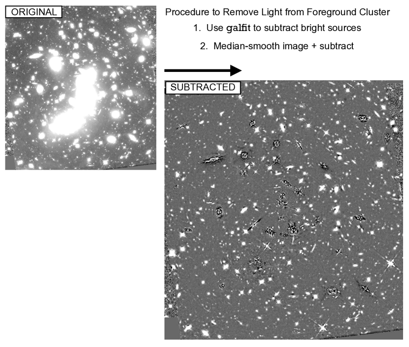
Figure 1.— Illustration of our procedure to subtract both light from the individual cluster galaxies and the cluster (i.e., the intracluster light). Our subtraction procedure (§2.2) involves two noteworthy steps: (1) subtraction of the bright foreground galaxies and (2) subtraction of the ICL. In subtracting bright foreground galaxies, we perform first careful profile fits using a Sérsic parameterization and secondly azimuthally-averaged fits to the light in various elliptical annuli. Finally, modeling of the intra-cluster light is performed based on two distinct median smoothings of the imaging data. Our intracluster-light subtraction procedure performs comparably well to other methodologies employed in the literature.

The broad organization of this paper is as follows. We begin by describing our data set and procedure for subtracting the foreground light from the cluster (§2). We then move onto a description of our procedure for constructing catalogs, selecting sources, and estimating the magnification factors (§3.1-§3.4), and then we finally compare our faint samples with previous samples from the literature (§3.5). Finally, in §4, we leverage our large samples to compute the surface density $\Sigma$ of galaxies at a given redshift vs. magnification factor $\mu$ and show how this can be used as a constraint on the faint-end slope of the $UV$ LF at various redshifts, the predictive power of the lensing models to high magnification factors, and other issues. §5 summarizes our results and provides a prospective for our future pursuits. For simplicity, we refer to the HST F275W, F336W, F435W, F606W, F814W, F105W, F125W, F140W, and F160W bands as $UV_{275}$, $U_{336}$, $B_{435}$, $V_{606}$, $I_{814}$, $Y_{105}$, $J_{125}$, $JH_{140}$, and $H_{160}$, respectively. Where necessary, we assume $\Omega_{0}=0.3$, $\Omega_{\Lambda}=0.7$, and $H_{0}=70\,\textrm{km/s/Mpc}$. All magnitudes are given in the AB system (Oke & Gunn 1983).

2. Data Sets and Background Subtraction

2.1. Data Sets

The primary data set for this study is the deep ultraviolet, optical, and near-infrared observations with HST over the Hubble Frontier Fields. The exposure times of the available HST observations vary somewhat from cluster to cluster, but includes at least 8, 8, 18, 10, 42, 24, 12, 10, and 24 orbits in the $UV_{275}$, $U_{336}$, $B_{435}$, $V_{606}$, $I_{814}$, $Y_{105}$, $J_{125}$, $JH_{140}$, and $H_{160}$ bands, respectively. We made use of the v1.0 reductions of the HFF provided by Koekemoer et al. (2014). We reduced the WFC3/UVIS observations using techniques similar to those used on the HDUV program (Oesch et al. 2018b), while ensuring that the final drizzled product was registered to the optical and near-IR reduced images from the public v1.0 HFF release. To account for the impact of extinction from our Galaxy along the line of sight to the clusters, we shifted the HST zeropoints that derived from Schlafly & Finkbeiner (2011) using the NASA/IPAC Extragalactic Database extinction calculator.

2.2. Background Subtraction Procedure

Searches for distant galaxies are made significantly more challenging due to the light from the foreground galaxy cluster. This includes both the intracluster light and light from bright cluster galaxies. Importantly, these foregrounds cause many interesting sources to be missed. This occurs as a result of confusion and foreground light being mistaken as light blueward of the Lyman break used to select high-redshift sources. These effects significantly complicate searches for distant galaxies.

A wide variety of different procedures have been developed to cope with the issue of intracluster light, e.g., Oesch et al. (2015), Atek et al. (2015b), Merlin et al. (2016), Livermore et al. (2017), Shipley et al. (2018), and Bhatawdekar et al. (2019). Many groups have made use of the SExtractor median-filtering algorithm to remove light from the cluster (Atek et al. 2015b), while making use of galfit (Peng et al. 2002, 2010) to subtract light from foreground cluster galaxies (Merlin et al. 2016; Bhatawdekar et al. 2019). Merlin et al. (2016) subtract light from the cluster adopting a modified Ferrer profile (Binney & Tremaine 1987) for the intra-cluster light. Livermore et al. (2017) used a wavelet procedure to subtract light from the cluster.

2.2.1 Fits to Individual Cluster Galaxies

The procedure we utilize involves first fitting to the light profiles of the 50 brightest foreground galaxies identified in the 3.4^′$\times$3.4^′ HST footprint over the cluster obtained with the ACS/WFC instrument.

The $I_{814}$-band images provide us with our starting point in fitting the spatial profile of individual foreground galaxies. Advantages of the $I_{814}$-band images are (1) their acquisition with the HST Advanced Camera for Surveys Wide Field Camera, which features a narrower PSF ($\sim$0.09^′′ FWHM) than with the WFC3/IR ($\gtrsim$0.15^′′ FWHM) and (2) the $I_{814}$ band’s probing the rest-frame optical light at 0.6$\mu$m in cluster galaxies, but not probing so red that the intracluster light substantially raises the background in most clusters.

Fits to the spatial profiles of foreground galaxies are performed with the galfit software using a Sérsic profile, allowing the source center, axial ratio, position angle, source size, Sérsic parameter, and total flux to vary. Our fits are based on a fit to a 2D grid of pixel flux values extending over the segmentation map for each source and extending 2^′′ further than this in each direction. After fitting the spatial profile of individual galaxies in the $I_{814}$ band, we repeat the fits in the other bands, only leaving the total flux as a free parameter in the fits while fixing the other Sérsic parameters to the values from our $I_{814}$ profile fits.

When subtracting these profile fits from the images, we compute the fit values at the horizontal and vertical boundaries of the two-dimensional region we are fitting. Using the fit values at the boundaries, we add back a linear interpolation of the fit values at the boundaries to avoid creating a square “hole” from the subtractions.

After using galfit to provide an initial subtraction of light from individual sources, we refined the subtraction by quantifying the average surface brightness $S(r_{A})$ in various elliptical annuli as a function of the major-axis radius. The elliptical annuli are defined using the position angle and axial ratio derived using our earlier galfit fits. The average surface brightness profiles $S(r_{A})$ are then smoothed along the major radial axis, and these smoothed elliptical annuli are then subtracted from the data.

Table 1Criteria Utilized in Selecting our $z\sim 2$-9 Samples

Sample	Criterion	HFF Clusters
$z$$\sim$2	(($UV_{275}$$-$$B_{435}$$>$1)$\vee$(($UV_{336}$$-$$V_{606}$$>$1)$\wedge$(SN($UV_{275}$)$<$2))$\wedge$	Abell 2744, MACS 0416, MACS0717
	($V_{606}$$-$$I_{814}$$<$0.3)$\wedge$(1.5$<$$z_{phot}$$<$2.5)$\wedge$(P($z$$>$1.2)$>$0.65)$\wedge$($\chi^{2}$$<$25)	MACS 1149, Abell S1063, Abell 370
$z$$\sim$3	(($UV_{275}$$-$$B_{435}$$>$1)$\vee$(($UV_{336}$$-$$V_{606}$$>$1)$\wedge$(SN($UV_{275}$)$<$2))$\wedge$	Abell 2744, MACS 0416, MACS0717
	($V_{606}$$-$$I_{814}$$<$0.3)$\wedge$(2.5$<$$z_{phot}$$<$3.5)$\wedge$(P($z$$>$1.2)$>$0.65)$\wedge$($\chi^{2}$$<$25)	MACS 1149, Abell S1063, Abell 370
$z$$\sim$4	$(B_{435}$$-$$V_{606}$$>$1)$\wedge$($I_{814}$$-$$J_{125}$$<$1)$\wedge$$(B_{435}$$-$$V_{606}$$>$1.6($I_{814}$$-$$J_{125}$)+1)$\wedge$	MACS0717, MACS1149
	($V_{606}$$-$$I_{814}$$<$0.5)$\wedge$[not in $z\sim 5$ selection]
$z$$\sim$5	$(V_{606}$$-$$I_{814}$$>$1.2)$\wedge$$(Y_{105}$$-$$H_{160}$$<$0.9)$\wedge$$(V_{606}$$-$$I_{814}$$>$1.2($Y_{105}$$-$$H_{160})$$+$1.32)$\wedge$	Abell 2744, MACS 0416, Abell S1063
	(SN($B$)$<$2)$\wedge$[$z\sim 5$ non-detection criterion]$\wedge$[not in $z\sim 6$ selection]	Abell 370
$z$$\sim$6	$(I_{814}$$-$$Y_{105}$$>$0.6)$\wedge$($Y_{105}$$-$$H_{160}$$<$0.45)$\wedge$$(I_{814}$$-$$Y_{105}$$>$0.6($Y_{105}$$-$$H_{160}$))$\wedge$	Abell 2744, MACS 0416, MACS0717
	($Y_{105}$$-$$H_{160}$$<$0.75($J_{125}$$-$$H_{160}$)+0.52)$\wedge$(SN($B_{435}$)$<$2)$\wedge$	MACS1149, Abell S1063, Abell 370
	([$z\sim 6$ non-detection criterion]$\vee$($V_{606}$$-$$Y_{105}$$>$2.5))$\wedge$
	($z_{phot}<6.3$)$\wedge$(P($z$$>$4.3)$>$0.65)$\wedge$[not in $z\sim 8$ selection]
$z$$\sim$7	$(I_{814}$$-$$Y_{105}$$>$0.6)$\wedge$($Y_{105}$$-$$H_{160}$$<$0.45)$\wedge$$(I_{814}$$-$$Y_{105}$$>$0.6($Y_{105}$$-$$H_{160}$))$\wedge$	Abell 2744, MACS 0416, MACS0717
	($Y_{105}$$-$$H_{160}$$<$0.75($J_{125}$$-$$H_{160}$)+0.52)$\wedge$(SN($B_{435}$)$<$2)$\wedge$	MACS1149, Abell S1063, Abell 370
	([$z\sim 6$ non-detection criterion]$\vee$($V_{606}$$-$$Y_{105}$$>$2.5))$\wedge$
	($z_{phot}>6.3$)$\wedge$(P($z$$>$4.3)$>$0.65)$\wedge$[not in $z\sim 8$ selection]
$z$$\sim$8	($Y_{105}$$-$$J_{125}$$>$0.45)$\wedge$$(J_{125}$$-$$H_{160}$$<$0.5)$\wedge$$(Y_{105}$$-$$J_{125}$$>$0.75($J_{125}$$-$$H_{160}$)$+$0.525)$\wedge$	Abell 2744, MACS 0416, MACS0717
	[$z\sim 8$ non-detection criterion]	MACS1149, Abell S1063, Abell 370
$z$$\sim$9	$(J_{125}$$-$$H_{160}$$>$1.2)$\wedge$$((H_{160}$$-$[3.6]$<$1.4)$\vee$$(\textrm{SN}([3.6])$$<$2))$\wedge$	Abell 2744, MACS 0416, MACS0717
	[$z\sim 9$ non-detection criterion]	MACS1149, Abell S1063, Abell 370

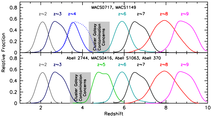
Figure 2.— The expected redshift distributions of our $z\sim 2$, 3, 4, 5, 6, 7, 8, and 9 selections over the HFF clusters for the two higher redshift ($z\sim 0.55$) clusters from the HFF program (MACS0717 and MACS1149: upper panel) and four HFF clusters at lower redshifts ($z\sim 0.3$-0.4: Abell 2744, MACS0416, Abell S1063, and Abell 370). These redshift distributions are computed from source injection and recovery experiments (as e.g. Bouwens et al. 2021a utilize). Due to the similar wavelength of the Lyman break in $z\sim 4$ and $z\sim 5$ galaxies to the Balmer/4000Å  break in foreground galaxies that make up the lower redshift and higher redshift clusters (see Figure 3), we only consider selections of $z\sim 4$ galaxies for the two higher redshift clusters and only consider selections of $z\sim 5$ galaxies for the four lower redshift clusters. The dotted blue line in the upper panel shows the expected $z\sim 4$ redshift distribution when utilizing our normal $z\sim 4$ selection criteria (which would be appropriate if a foreground cluster were not present in our search field).

2.2.2 Modeling of the Intracluster Light

After having modeled and subtracted the light from the brightest 50 foreground galaxies, the next step we utilize is to remove the extended intracluster light by subtracting a median-smoothed image of the cluster – which we implement in two steps. Our approach follows the SExtractor (Bertin & Arnouts 1996) implementation of this algorithm. The procedure is first to break up the image into grid cells of some fixed individual dimension and set the nominal background level for a cell to be 3 times the mean minus two times the median. Then, the next step is to execute a 3$\times$3 median smoothing on this grid and construct an ICL model by splining over individual cells in the grid. Finally, this ICL model is subtracted from the data itself.

In our initial implementation of the subtraction of this median-smoothed image, we adopted a relatively large angular size for individual cells in the grid, i.e., 1.2^′′, since we found that had the least impact on the total flux measurements we made for individual sources. We, however, found that this did not produce a flat background across the full image. In particular, around bright galaxies, there was some noticeable “ringing” in the background, making the recovery of sources in the affected regions more challenging.

To improve the flattening of the background in the specific regions of the image impacted by such ringing, we explicitly demarcated the affected regions with ds9. We repeated our determination of a median-smoothed image using significantly smaller grid cells, i.e., with dimension 0.4^′′, and repeated our construction of a median-smoothed image for the cluster. Not surprisingly, after subtraction of this high-resolution median-smoothed image from the original, much less ringing is evident around bright foreground galaxies. This approach, however, results in the systematic reduction (by $\sim$0.1-0.15 mag) in the measured flux of sources, due to the subtraction of flux on larger spatial scales.

To maximize the completeness of the present search results around bright sources while maximizing the accuracy of the photometry in more crowded regions, we make use of two different median-smoothed images to subtract the ICL light: (1) using the image with the coarser grid cells in the less crowded regions, which constitute 80% of the HFF WFC3/IR search area, and (2) using the image with finer grid cells in the more crowded region, constituting 20% of the image.

2.2.3 Summary

The ICL subtraction that the above procedure delivers is illustrated in Figure  1, and it is clear that we obtain a good subtraction of the foreground light from the cluster and under the brightest sources in the cluster, without substantial “ringing” in the immediate vicinity of various foreground sources.

In Bouwens et al. (2017b: Appendix A), we already demonstrated that with our background subtraction algorithm (now described in detail here) we were able to identify a comparable number of $z\sim 6$-8 galaxies to that found in Merlin et al. (2016) and Livermore et al. (2017). The source numbers presented in §3.5 provide further evidence that our algorithm works well.

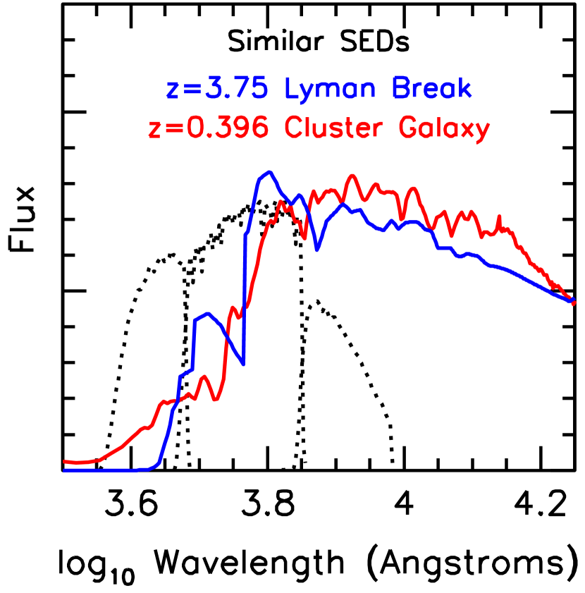
Figure 3.— Illustration of how similar the SED shape of a $z\sim 3.75$ star-forming galaxy (blue) is to that of an evolved galaxy at $z=0.396$ (red). The dotted black lines show the transmission curves of the optical $B_{435}$, $V_{606}$, and $I_{814}$ filters utilized for the six clusters in the HFF program. As a result of the similar SED shapes of $z\sim 4$ Lyman-break galaxies to evolved galaxies in the foreground clusters, contamination poses a significant challenge for $z\sim 4$ selections from the HFF program.

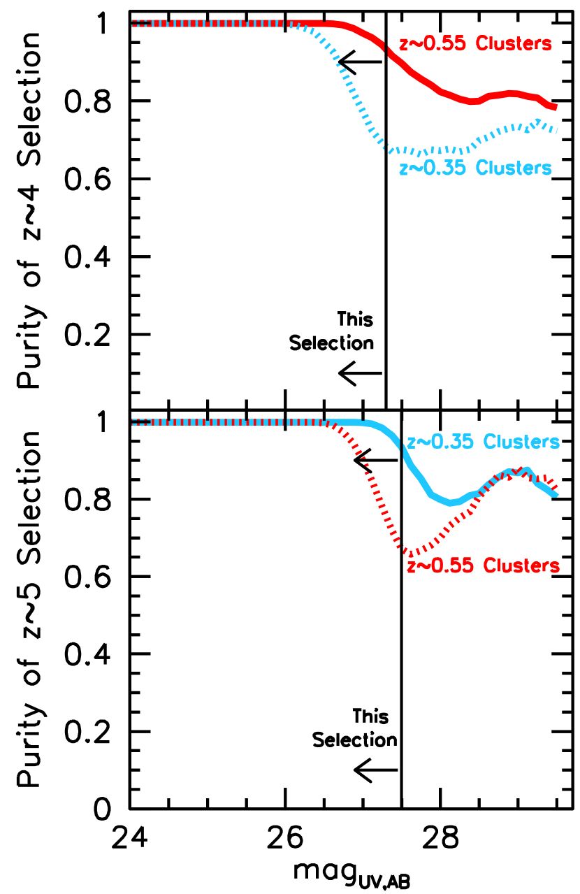
Figure 4.— Illustration of the estimated purity of our $z\sim 4$ and $z\sim 5$ galaxy selections (upper and lower panels, respectively) as a function of apparent magnitude behind the HFF clusters. Results are shown both using the $z\sim 0.35$ and $z\sim 0.55$ HFF clusters (blue and red lines, respectively). See §3.3 for a description of the simulations. Despite the challenges created by foreground cluster galaxies contaminating selections of star-forming galaxies at $z\sim 4$-5, relatively clean selections are possible if (1) only sources brighter than 27.3 mag at $z\sim 4$ and 27.5 mag at $z\sim 5$ (vertical lines) are included and (2) only utilizing those clusters where the Lyman break occurs across a different set of broadband filters than the 4000Å/Balmer break.

3. Construction of Faint Samples

3.1. Catalog Construction

As in previous work (Bouwens et al. 2011, 2015), we use the SExtractor software (Bertin & Arnouts 1996) to handle source detection and photometry. SExtractor is run in dual-image mode, with the detection image taken to equal the square root of $\chi^{2}$ image (Szalay et al. 1999: similar to a coadded image) constructed from one or more HST bands, depending on the redshift of galaxy we are searching. We use the $B_{435}V_{606}I_{814}$ images for our $z\sim 2$ and $z\sim 3$ selections, the $Y_{105}$, $J_{125}$, $JH_{140}$ and $H_{160}$ images for our $z\sim 4$, $z\sim 5$, $z\sim 6$, and $z\sim 7$ selections, the $J_{125}$, $JH_{140}$, and $H_{160}$ images for our $z\sim 8$ selection, and the $JH_{140}$ and $H_{160}$ bands for our $z\sim 9$ selection. Color measurements are made in small scalable apertures (Kron [1980] factor of 1.2), after PSF-matching the observations. The PSF matching is done to the $I_{814}$ band (if the color consists entirely of optical bands) or the $H_{160}$ band (if the color also includes a near-infrared band).

Total-magnitude measurements are made by correcting the smaller-scalable aperture flux measurements to account for light outside these apertures. Two corrections are considered. The first accounts for the excess flux measured in a larger-scalable aperture (Kron [1980] factor of 2.5) relative to the smaller-scalable aperture and second to account for the light on the wings on the PSF (typically a $\sim$0.15-0.25 mag correction). The second correction is made using the tabulated encircled energy distributions (Dressel et al. 2012).

In selecting $z\sim 9$ galaxies over our fields, it is useful to be able to make use of the sensitive Spitzer/IRAC observations that have been obtained over the fields. Due to the relatively broad PSF of Spitzer/IRAC relative to the surface density of sources on the sky, source crowding is an issue in measuring fluxes for sources. As in much of our previous work, we use the mophongo software for this endeavor (Labbé et al. 2010a, 2010b, 2013, 2015). In executing this activity, Mophongo considers the positions and morphologies of sources in the HST data as well as an HST-to-IRAC PSF matching kernel to model the spatial distribution of light from each source. After fitting for the flux of each source, light from neighboring sources is subtracted, and then aperture photometry is performed to measure the flux from a source within a given aperture. That measured flux is then corrected to total based on the form of the PSF.

3.2. Source Selection

In selecting $z=2$-9 galaxies from the parallel and cluster fields that make up the HFF program, we pursue a very similar approach as to what we have used in Bouwens et al. (2021a) over the HDUV fields and HFF fields. A summary of the selection criteria we utilize is presented in Table 1 for our $z\sim 2$, 3, 4, 5, 6, 7, 8, and 9 samples.

Figure 2 shows the expected redshift distributions of our $z\sim 2$, 3, 4, 5, 6, 7, 8, and 9 selections for the six HFF clusters considered here. The expected redshift distributions are as derived in Bouwens et al. (2021a) and make use of the same $UV$-continuum slope $\beta$ and size-luminosity scalings as implemented there, with the exception of $z\sim 4$ as discussed below.

The best-fit photometric redshifts and $\chi^{2}$ we derive that play a role in our $z\sim 2$-3 and $z\sim 6$-7 selections use the EAzY photometric redshift software (Brammer et al. 2008). The SED templates utilized with EAzY were the EAzY_v1.0 set together with SED templates from the Galaxy Evolutionary Synthesis Models (GALEV: Kotulla et al. 2009). Emission lines were added to the later templates assuming a rest-frame EW of 1300Å for H$\alpha$ with line ratios given by the $0.2Z_{\odot}$ Anders & Fritze-v. Alvensleben (2003) prescription. When deriving photometric redshift constraints and computing a $\chi^{2}$, an additional 7% uncertainty in our flux measurements is assumed to allow for small systematic differences between the observed and model SEDs and small systematics in the photometry.

Candidate galaxies at $z\sim 6$-7, $z\sim 8$, and $z\sim 9$ are required to have a signal-to-noise ratio of 6 in a stack of the available WFC3/IR observations in the $Y_{105}J_{125}JH_{140}H_{160}$, $J_{125}JH_{140}H_{160}$, and $JH_{140}H_{160}$ bands, respectively. Sources which correspond to diffraction spikes are the clear result of an elevated background around a bright source (e.g., for a bright elliptical galaxy), or correspond to other artifacts in the data are removed by visual inspection.

All bright ($H_{160,AB}<27$) sources with SExtractor stellarity parameters in excess of 0.9 (where 0 and 1 correspond to extended and point sources, respectively) are removed. Sources where the stellarity parameter is in excess of 0.6 are also removed, if the HST photometry is much better fit with SEDs of low-mass stars ($\Delta\chi^{2}>2$) from the SpeX library (Burgasser et al. 2004) than with a linear combination of galaxy templates from EAzY (Brammer et al. 2008).

To ensure our $z\sim 9$ sample is not contaminated by lower-redshift sources with red spectral slopes, we made use of the available 3.6$\mu$m Spitzer/IRAC observations. Sources were excluded from our selection if they were detected at $3\sigma$ in the 3.6$\mu$m observations and had $H_{160}-[3.6]$ colors redder than 0.8 mag.

To maximize the completeness in selecting sources for our $z\sim 6$-9 catalogs (where the numbers are small), we considered five different background subtraction algorithms, each using a different angular size for the SExtractor background mesh, and regenerated our source catalogs and $z\sim 6$-9 selections from each. This reduces the number of sources that would be missed due to the deblending choices made by SExtractor in constructing a given catalog, thereby maximizing the robustness of our results.

Table 2Lensing Models Utilized (see also §3.4)

Cluster	Model	Version
Abell 2744	CATS (P)	v4.1
	Sharon/Johnson (P)	v4
	Keeton (P)	v4
	GLAFIC (P)	v4
	Zitrin/NFW (P)	v3
	Grale (NP)	v4
	Bradac (NP)	v2
	Zitrim-LTM-Gauss (NP)	v3
	Diego (NP)	v4.1
MACS0416	CATS (P)	v4.1
	Sharon/Johnson (P)	v4
	Keeton (P)	v4
	GLAFIC (P)	v4
	Zitrin/NFW (P)	v3
	Caminha (P)	v4
	Grale (NP)	v4
	Bradac (NP)	v3
	Zitrim-LTM-Gauss (NP)	v3
	Diego (NP)	v4.1
MACS0717	CATS (P)	v4.1
	Sharon/Johnson (P)	v4
	Keeton (P)	v4
	GLAFIC (P)	v3
	Grale (NP)	v4.1
	Diego (NP)	v4.1
MACS1149	CATS (P)	v4.1
	Sharon/Johnson (P)	v4
	Keeton (P)	v4
	GLAFIC (P)	v3
	Grale (NP)	v4
	Diego (NP)	v4.1
Abell 370	CATS (P)	v4
	Sharon/Johnson (P)	v4
	Keeton (P)	v4
	GLAFIC (P)	v4
	Bradac (NP)	v4.1
	Grale (NP)	v4
	Diego (NP)	v4.1
Abell S1063	CATS (P)	v4.1
	Sharon/Johnson (P)	v4
	Keeton (P)	v4
	GLAFIC (P)	v4
	Caminha (P)	v4
	Grale (NP)	v4
	Diego (NP)	v4.1

3.3. Selection of Galaxies at $z\sim 4$-5

Selecting galaxies at $z\sim 4$-5 behind the galaxy clusters in the HFF program is significantly more challenging than at $z\gtrsim 6$ and $z\sim 2$-3 due to the cluster galaxies themselves. Many cluster galaxies show prominent 4000Å  and Balmer breaks which fall between the $B_{435}$ and $V_{606}$ bands or in the center of the $V_{606}$ band. As Figure 3 illustrates, this feature can look very similar to the Lyman break for a $z\sim 4$ galaxy. This makes the selection of $z\sim 4$ galaxies especially challenging for the four lowest-redshift clusters in the HFF program lying between $z\sim 0.3$ and $z\sim 0.4$, i.e., Abell 2744, MACS0416, Abell S1063, and Abell 370.

Given these challenges, we select $z\sim 4$ galaxies by targeting the two clusters where the 4000Å  or Balmer breaks are redshifted significantly through the $V_{606}$ band, i.e., MACS0717 ($z=0.543$) and MACS1149 ($z=0.547$), such that the 4000Å/Balmer spectral break in cluster galaxies is approximately midway through the $V_{606}$ band. Given that cluster galaxies have $V_{606}-I_{814}$ and $B_{435}-V_{606}$ colors somewhat similar to $z\sim 5$ galaxies, one can achieve the most robust selection of $z\sim 4$ galaxies by targeting galaxies over the range $z\sim 3.5$-4.0, with smaller $V_{606}-I_{814}$ breaks, i.e., where $(V_{606}-I_{814}<0.5)$.

By contrast, $z\sim 5$ galaxies can be best selected by focusing on the four clusters where the 4000Å  or Balmer breaks are not as significantly redshifted through the $V_{606}$ band, i.e., Abell 2744 ($z=0.308$), MACS 0416 ($z=0.396$), Abell S1063 ($z=0.348$), and Abell 370 ($z=0.375$). The $z\sim 5$ criteria we utilize (Table 1) are identical to those presented in Bouwens et al. (2021a).

To minimize the impact of noise in causing sources from the foreground clusters to satisfy our $z\sim 4$-5 selection criteria, we only include $z\sim 4$ and $z\sim 5$ sources brighter than $H_{160,AB}\sim 27.3$ mag and 27.5 mag, respectively, in our selection. We arrived at these magnitude limits using Monte-Carlo simulations where we added photometric noise to the $z\sim 0$ Coleman et al. (1980) E/S0, Sab, and Imm templates placed at the approximate redshifts of the HFF clusters and a 100 Myr Bruzual & Charlot (2003) starburst template placed at $z\sim 3.75$ and $z\sim 5$. Then, to estimate an approximate purity at a given magnitude level, we divided the estimated number of high-redshift galaxies by that number plus the expected contamination from cluster galaxies. For these estimates, we assume the surface density of foreground cluster galaxies is 10$\times$ higher than the high-redshift population to be conservative.

The result is shown in Figure 4 for both our $z\sim 4$ and $z\sim 5$, and it is clear that we can obtain a much cleaner selection of $z\sim 4$ and 5 galaxies if we restrict ourselves to galaxies brighter than 27.3 mag and 27.5 mag, respectively. As a check on our decision to select $z\sim 4$ galaxies from the two highest redshift clusters, i.e., MACS0717 and MACS1149, and $z\sim 5$ galaxies from the four lower redshift clusters, we repeated these simulations for the clusters excluded from our $z\sim 4$ and $z\sim 5$ selections (i.e., where the Lyman break for $z\sim 4$-5 galaxies lies across a similar set of bands to the 4000Å/Balmer breaks for cluster galaxies). We see significant contamination setting in $\sim$1 mag brighter for these clusters and being 2-10$\times$ higher. Based on these results, it clearly seems to have been prudent to have excluded these specific cluster fields from our $z\sim 4$ and $z\sim 5$ selections.

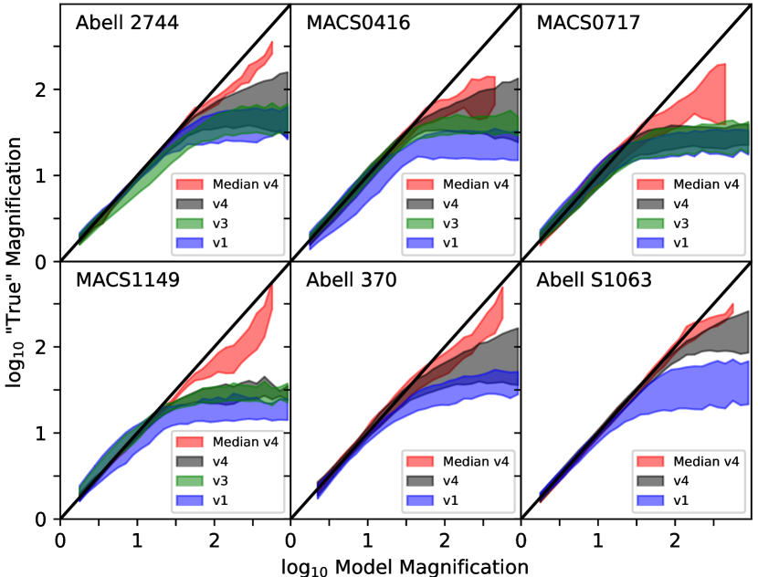
Figure 5.— Illustration of how well the model magnification factors from individual parametric lensing models (shown along horizontal axis) are able to predict the magnification factors (shown on vertical axis) for the v4 CATS, Sharon/Johnson, Keeton, and GLAFIC models of the same HFF cluster (see §3.4.1). The blue, green, and black-shaded regions show the $1\sigma$ range in mean magnification factors predicted using independent v1, v3, and v4 models, respectively. All sources are assumed to be at $z=6$. The red-shaded region shows the $1\sigma$ range in mean magnification factors predicted using the median of the other v4 parametric models (except the v4 model being predicted). These shaded regions demonstrate the individual magnification models are effective in predicting the magnification factors to values of $\sim$20-50, depending on the HFF cluster. In general, the v4 models exhibit better predictive power than the v1 models, particularly for MACS0416, MACS1149, Abell 370, and Abell S1063. The median v4 models exhibit even better predictive power, being effective in predicting the magnification factors to values of $\sim$100 and in some cases higher.

3.4. Model Magnification Factors

To interpret the faint high-redshift sources we have identified behind the HFF lensing clusters, we must estimate the degree to which each source is magnified by the foreground cluster.

Fortunately, in parallel with the acquisition of deep HST observations from the HFF program, a variety of groups have been involved in constructing lensing models for the HFF clusters (e.g., Bradac et al. 2009; Diego et al. 2005, 2007, 2015a, 2015b, 2018; , Keeton 2010; Liesenborgs et al. 2006; Mahler et al. 2018; Merten et al. 2015, Richard et al. 2014; Zitrin et al. 2012, 2015). At present, all six clusters have anywhere between 6 to 10 models available for them (Table 2) using the latest (v3/v4) sets of constraints. These constraints include large numbers of multiple image pairs available from the HFF observations, as well as spectroscopic redshift constraints mentioned earlier.

Magnification of a source at a particular redshift can be calculated on the basis of the convergence $\kappa$ and shear $\gamma$ maps numerous teams have derived in modeling background sources in the HFF data:

$$\mu=\frac{1}{|(1-\kappa)^{2}-\gamma^{2})|}$$ (1)

Note that the $\gamma$ and $\kappa$ values in the above equation are not simply the values in the published maps, but also include multiplication by a $D_{LS}/D_{S}$ factor, where $D_{LS}$ is the angular-diameter distance from the lens to the lensed background source, while $D_{S}$ is the angular-diameter distance to the lensed background source.

3.4.1 Testing the Reliability of the Magnification Factors from the Public Models

Prior to making use of the public magnification models, it is useful to ask ourselves over which range of magnification factors these models can be trusted to give reliable results. There have been several earlier studies that have looked into this in some detail (e.g., Meneghetti et al. 2017; Priewe et al. 2017; Bouwens et al. 2017a), and one consensus conclusion from these studies has been that the parametric magnification models show excellent predictive power to at least a magnification factor of 30.

Following the release of v3 magnification models, more spectroscopic redshift measurements on lensed galaxies behind the HFF clusters have been made available. The release of the v4 lensing models should provide even more accurate constraints on the magnification factor for individual sources than the v3 models. It therefore makes sense to reassess how well various public lensing models predict the true magnification factors of sources behind the HFF clusters.

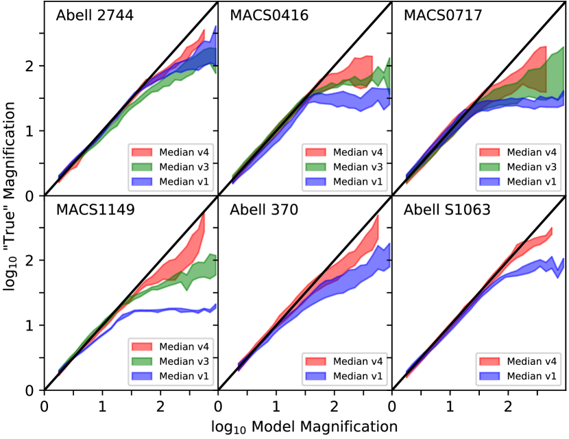
Figure 6.— An illustration of how well the median of the v1, v3, and v4 parametric magnification models are able to predict the “true” magnification factor (as represented by one of the v4 parametric models: see §3.4.1). The blue, green, and red shaded regions show the $1\sigma$ range of mean magnification factors recovered for v4 models at a given median magnification factor from the v1, v3, and v4 parametric models, respectively. All sources are assumed to be at $z=6$. There is a clear improvement in the predictive power of the median models from v1 to v4.

Leveraging the approach presented in §3.1 of Bouwens et al. (2017a), we test the predictive power of the lensing model by treating one of the many parametric lensing models as the truth and then testing how well the other lensing models are able to predict its magnification factors. As each model represents a comparably realistic representation of the true lensing model, this is a reasonable way to proceed. Given the large number of public parametric models available for each of the individual HFF clusters, we can make use of a significant number of model pairs to assess the predictive power of individual models.

In Figure 5, we present the results we obtain of this exercise using the magnification factors from individual v1, v3, and v4 models to predict the magnification factors of separate v4 models for all HFF clusters. For simplicity, all sources are assumed to have a redshift of $z=6$ through this exercise. To avoid favoring any one of the public lensing models, each family of the v4 lensing models is alternatively treated as the truth, and then the mean logarithmic magnification factor in the “truth” model is calculated as a function of the magnification factor for a different lensing model. Making use of the many different pairs of lensing models, one treated as the “truth” and the other treated as a predictive model, we can calculate a mean magnification and $1\sigma$ scatter about the “true” magnification, as a function of the model magnification factor.

Figure 7.— (left) Comparison of the magnification factors reported in the literature (Zitrin et al. 2014; Infante et al. 2015; Livermore et al. 2017; Ishigaki et al. 2018: red circles) for specific $z\sim 6$-10 galaxies to values $<$100 (horizontal axis) and median magnification factors from the v4 parametric models (see §3.4.1). The green shaded region shows the expected $1\sigma$ range in predictive power of the median v3 models for the magnification of sources vs. that seen in v4 parametric models. The shaded red region shows $1\sigma$ scatter in the v4 magnifications in the median v4 magnification vs. the magnification factors reported in various literature studies. Below a model magnification factor of $\sim$50, both results in the literature and the median v3 models agree very well with the v4 model results; above a magnification factor of 50, the magnification factor for sources, as estimated by the v4 models, saturates around values of $\sim$50 to 100. Both the points and shaded regions for magnification factors $>$50 are shown with a lighter shading to reflect the lesser reliability of magnification factors in this regime. (right) Similar to left figure, but showing the ratio of the median v4 magnification and the reported magnification factors.

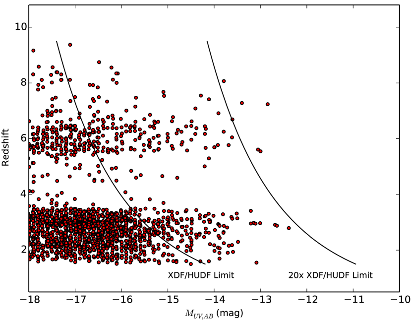
Figure 8.— Estimated $UV$ luminosity of candidate star-forming galaxies in our HFF samples vs. redshift (filled red circles). The two solid lines show the $UV$ luminosities probed by the 30-mag XDF/HUDF data and $20\times$ fainter than the XDF/HUDF data. Clearly, the full HFF data set contains a large numbers of candidate ultra-faint ($\gtrsim-$14 mag) galaxies from $z\sim 8$ to $z\sim 2$. The much smaller number of sources in our samples at $z\sim 3.5$-5.5 is a direct result of the much more conservative criteria required to select such sources free of contamination.

In general, the model magnification factors predict the “true” magnification factors to a magnification factor of $\sim$20-30 and then lose their predictive power at magnification factors of $\sim$20 (MACS1149), $\sim$30 (MACS0717) to $\sim$50-100 (Abell 2744, MACS 0416, Abell 370, Abell S1063). The predictive power of the individual v4 models appears to be higher, as expected, than the v1 models for Abell 2744, MACS 0416, Abell 370, and Abell S1063, with the most significant improvement seen for the Abell S1063 models.

Table 3Samples of $z=2$-10 Galaxies found over the six HFF cluster fields (including Oesch et al. 2018a selection)

Cluster	Area [arcmin2]	$z\sim 2$	$z\sim 3$	$z\sim 4$	$z\sim 5$	$z\sim 6$	$z\sim 7$	$z\sim 8$	$z\sim 9$	$z\sim 10$
Abell 2744	4.9	157	233	—	27	49	25	15	4	2
MACS0416	4.9	215	233	—	7	50	26	10	6	0
MACS0717	4.9	81	160	32	—	26	14	9	0	0
MACS1149	4.9	134	195	36	—	52	21	5	2	0
Abell S1063	4.9	96	203	—	11	62	28	6	3	0
Abell 370	4.9	82	152	—	14	35	11	6	1	0
Total	29.4	765	1176	68	59	274	125	51	16	2

In Figure 5, we also show how well the median of the v4 magnification models predict the magnification factors of the v4 magnification model not included in the median. For all six HFF clusters, the median magnification model is successful at predicting the “true” magnification to values of $\gtrsim$40, with the best performance achieved for Abell S1063, with the predictive power extending to values of $\sim$100.

In Figure 6, we show how well the median of the v1, v3, and v4 magnification models predict the magnification factors of the v4 models. For five of the six clusters, except perhaps Abell 2744, there is a clear improvement in the predictive power of the median v4 model over the median v1 model. For four of the clusters, i.e., Abell 2744, MACS 0416, Abell 370, and Abell S1063, the median of the v4 magnification models is successful at predicting the magnification factors to values of $\gtrsim$80.

A number of previous studies have explicitly tabulated the magnification factors they derived for $z\sim 6$-10 galaxies (Zitrin et al. 2014; Infante et al. 2015; Livermore et al. 2017; Ishigaki et al. 2018) using either their own lensing models or the publicly available HFF lensing models. As all but one of these models predated the latest v4 models and made use of a smaller set of constraints, comparison of these published magnification factors with the v4 results provide us with a measure of the robustness of the magnification factors, after improvements are made to the models.

Figure 7 compares various published magnification factors from the literature (Zitrin et al. 2014; Infante et al. 2015; Livermore et al. 2017; Ishigaki et al. 2018) with the median of the v4 parametric models. The green-shaded region shows the expected $1\sigma$ range in predictive power of the median v3 models for the magnification of sources vs. that seen in v4 parametric models. The green-shaded region is a marginalized version of the green shaded region shown in Figure 5 over the first four clusters (which feature v3 models). The red shaded area shows the $\pm$1$\sigma$ range in median v4 magnification factors found for sources within a 0.2-dex range of published magnification factors.

Encouragingly, we find that the published magnification factors are consistent with the median v4 magnifications to values of $\sim$40-50. For higher magnification factors, i.e., $>$60, we find that the reported magnifications magnifications are less robust, and the median magnifications we find for those sources using the v4 parametric models lie in the range $\sim$40 to $\sim$100.

3.4.2 The Challenge of Identifying Especially Faint Galaxies

One area where both new models make quite a difference is in our quest for the faintest galaxies. These are important for helping constrain both the faint end of the luminosity function and also for the role they play in distinguishing various galaxy formation scenarios. The challenge, however, of working at high magnifications in a regime where the models are both improving and evolving can be seen from the results for the very faintest objects. As such, it is interesting to reconsider the faintest sources found with earlier models to have exceptionally low luminosities, i.e., $\gtrsim-15$ at $z\sim 6$-9 and $\gtrsim-16$ at $z\sim 9$. There are $>$20 such sources presented thus far in the literature. For this exercise, we use the same methods and lensing models as we use here.

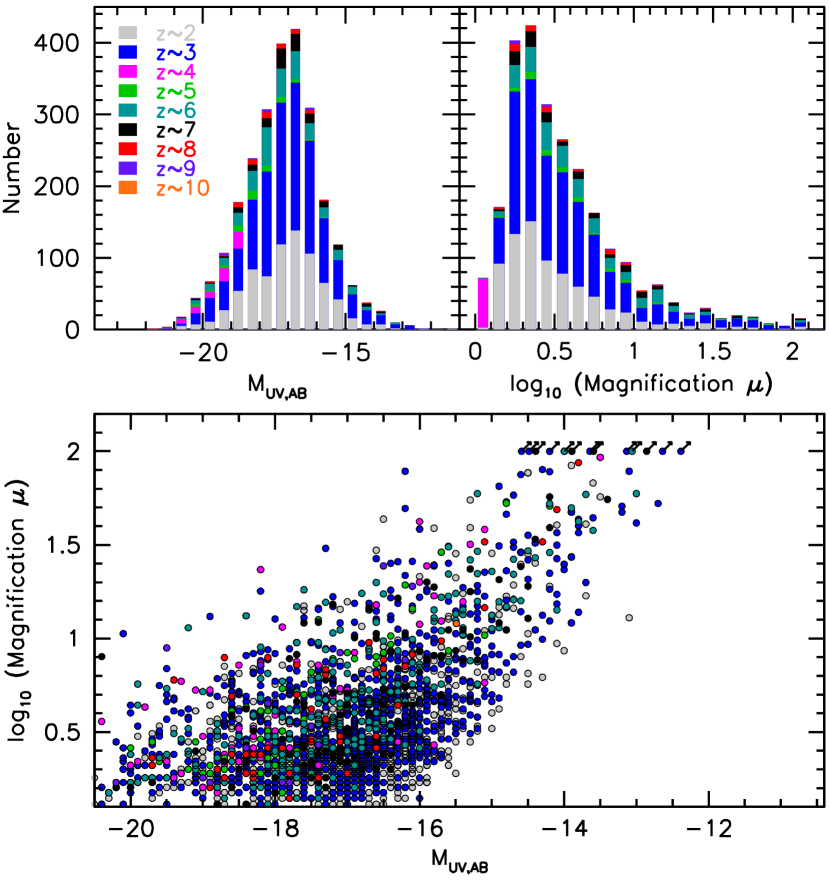
Figure 9.— Number of $z\sim 2$, $z\sim 3$, $z\sim 4$, $z\sim 5$, $z\sim 6$, $z\sim 7$, $z\sim 8$, $z\sim 9$, and $z\sim 10$ sources (grey, blue, magenta, green, cyan, black, red, purple, and orange histograms, respectively) identified over all six HFF clusters and parallel fields vs. the inferred absolute magnitude (upper left panel) and model magnification factor (upper right panel). We impose a hard upper limit of 100 on the allowed magnification factor of sources, affecting just 16 sources ($<$1% of the total). (lower panel) Median model magnification factors vs. absolute magnitudes for sources in our $z\sim 2$, $z\sim 3$, $z\sim 4$, $z\sim 5$, $z\sim 6$, $z\sim 7$, $z\sim 8$, $z\sim 9$, and $z\sim 10$ samples (grey, blue, magenta, green, cyan, black, red, purple, and orange points, respectively).

What we find is that the faintest galaxies from several previous studies, those reported to be fainter than approximately $-$15.5 mag and $-$14.5 mag, are $\sim$0.5 mag and 0.7 mag brighter, respectively. In the median, the faint sources are estimated to be 0.4 mag and 0.5 mag brighter, respectively. In addition, we find that few of the sources with nominal $UV$ luminosities fainter than $-$14 mag are estimated to be fainter than $-$14 mag using the median v4 parametric models.

Even with the v4 updates to the magnification estimates to individual sources, the latest models will likely be revised in the future. As such, caution is required in considering the implications of the faintest sources in the current compilation. While use of median magnification models should improve the robustness of the magnification estimates, many of the models make use of similar assumptions and similar observational constraints. As a result, the true systematic uncertainties could well be larger than indicated by the dispersion in model results.

3.4.3 Fiducial Magnification Factors

For our fiducial estimate of the magnification for individual sources, we take the median of the magnification estimates from the v4 parametric models, i.e., GLAFIC, CATS, Sharon/Johnson, Zitrin-NFW, Keeton, and Caminha (where available) since the parametric models in general have proven to be among the best performing models for the HFF comparison project (Meneghetti et al. 2017). Included in our estimates of the median magnification factor are the best $\kappa$ and $\gamma$ maps and the other models in the associated Markov Chain Monte Carlo (MCMC) chain. Based on the range in magnifications from the parametric models, we estimate 68% confidence intervals on the model magnification factors. In cases where both a v4 and v4.1 model exists, both are considered equally in computing a median for that specific flavor of lensing model.

While the tests in the previous subsection support the robustness of magnification estimates to factors of $\gtrsim$40 and have utility in predicting the magnification factors to values of $\sim$100, they also cast doubt on the robustness of these estimates when the magnification factors exceed 100. In the interest of maximizing the robustness of the results we present, we adopt a maximum magnification factor of 100 for our analyses and also for our companion paper on the $UV$ LFs (R. Bouwens et al. 2022, in prep). For the few sources in our catalogs where the median magnification factors we derive exceed 100, i.e., 16 sources, we explicitly set the magnification estimates of those sources equal to 100 (as can also be seen in Figure 9 from §3.5).

Table 4A complete list of the sources included in the $z\sim 2$, $z\sim 3$, $z\sim 4$, $z\sim 5$, $z\sim 6$, $z\sim 7$, $z\sim 8$, $z\sim 9$, and $z\sim 10$ samples from the present selection and that of Oesch et al. 2018a

ID	R.A.	Dec	$m_{AB}$	Sample	Data Set	$z_{phot}$	$\mu_{Median-Parametric}$
A2744275-4227525020	00:14:22.75	$-$30:25:02.0	27.45	2	17	2.44	2.6${}_{-0.3}^{+0.1}$
A2744275-4236124532	00:14:23.61	$-$30:24:53.2	28.45	2	17	2.33	3.2${}_{-0.3}^{+0.3}$
A2744275-4245824489	00:14:24.58	$-$30:24:48.9	28.22	2	17	2.30	3.0${}_{-0.1}^{+0.4}$
A2744275-4239224503	00:14:23.92	$-$30:24:50.3	25.28	2	17	1.93	3.3${}_{-0.2}^{+0.4}$
A2744275-4240424495	00:14:24.04	$-$30:24:49.5	24.92	2	17	1.74	3.2${}_{-0.2}^{+0.4}$
A2744275-4224124478	00:14:22.41	$-$30:24:47.8	28.60	2	17	2.30	4.6${}_{-0.6}^{+0.3}$
A2744275-4239924345	00:14:23.99	$-$30:24:34.5	28.00	2	17	2.15	6.7${}_{-1.4}^{+1.6}$
A2744275-4225724288	00:14:22.57	$-$30:24:28.8	26.26	2	17	2.10	3.7${}_{-0.3}^{+0.3}$
A2744275-4230424248	00:14:23.04	$-$30:24:24.8	29.49	2	17	2.21	4.8${}_{-0.3}^{+0.8}$
A2744275-4226724234	00:14:22.67	$-$30:24:23.4	28.91	2	17	1.95	2.5${}_{-0.2}^{+0.7}$

3.5. Final Samples of $z\sim 2$-9 Galaxies

The present procedure resulted in the construction of very large samples of $z\sim 2$-9 galaxies. Our $z\sim 2$, $z\sim 3$, $z\sim 4$, $z\sim 5$, $z\sim 6$, $z\sim 7$, $z\sim 8$, and $z\sim 9$ samples include 765, 1176, 68, 59, 274, 125, 51, and 16 sources, respectively. The total number of sources in the collective $z\sim 2$-10 sample from this work and that of Oesch et al. (2018a) is 2536. These results are summarized in Table 3.

With our total sample of sources stretching from $z=2$ to $z=10$, it is interesting to show the luminosities that we potentially probe with HFF program. In Figure 8, we present the $UV$ luminosities of sources in our selection vs. the photometric redshift we derive from EAzY. Remarkably, for our selection (and that of Oesch et al. 2018a), we probe to $-$12.4 mag at $z\sim 3$ and $-$12.9 mag at $z\sim 7$. For context, we also present a black line illustrating the $UV$ luminosity that we probe at 30 mag in the eXtreme Deep Field (XDF) / Hubble Ultra Deep Field (HUDF: Beckwith et al. 2006; Illingworth et al. 2013; Koekemoer et al. 2013). From this figure, it is clear that with the HFFs, we probe $\gtrsim$20$\times$ fainter than what is possible in the XDF/HUDF.

We give further insights into our sample in Figure 9. The upper left and right panels show the cumulative number of star-forming galaxies at $z=2$, 3, 4, 5, 6, 7, 8, 9, and 10 as a function of $UV$ luminosity and magnification, respectively, while the distribution in magnification and $UV$ luminosity is shown in lower panel of the same figure. A complete compilation of the present sample of $z=2$-9 galaxy candidates is provided in Table 4.

The present selection of $z\sim 2$-9 galaxies is $\sim$2-3$\times$ larger than previous selections at these redshifts. Previously, Alavi et al. (2017) had identified 297 z$\sim$1.0-1.6, 318 z$\sim$1.6-2.2, and 278 z$\sim$2.2-3.0 galaxies using the HST observations over three lensing clusters: Abell 1689 and two HFF clusters Abell 2744 and MACS0717. At $z\geq 6$, Ishigaki et al. (2018) had identified 140 $z\sim 6$-7, 27 $z\sim 8$, and 14 $z\sim 9$ galaxies, respectively, over all six clusters. Atek et al. (2018) report finding 300 $z\sim 6$-7 galaxies over the six HFF clusters, while Leung et al. (2018) report finding 260 $z\geq 4.75$ galaxies. Yue et al. (2018) report a total sample of 272 $z=5$-9.5 galaxies from the first four HFF clusters. Atek et al. (2015b) had identified some 119 $z\sim 6$-7 galaxies and 13 $z\sim 8$ galaxies as part of their HFF selections over three clusters, while Livermore et al. (2017) identified 105 $z\sim 6$, 40 $z\sim 7$, and 16 $z\sim 8$ galaxies behind Abell 2744 and MACS0416. Zheng et al. (2014), Infante et al. (2015), Laporte et al. (2016), Zheng et al. (2017) report 117 $z=6$-10 sources in total from the first 4 HFF cluster and parallel fields.

4. $z=2$-9 Galaxy Surface Density Results

The purpose of this section will be to quantify the dependence of the surface density of lensed $z=2$-9 galaxies on the magnification factor and then to use the results to draw conclusions about the physical characteristics of faint $z=2$-9 galaxies. The dependence of the surface density of lensed galaxies on the magnification factor is frequently referred to as the magnification bias in the literature (Turner et al. 1984; Broadhurst 1995, Broadhurst et al. 2005).

The magnification bias is often expressed as the ratio $N^{\prime}(<m)/N_{o}(<m)=\mu^{2.5S-1}$ where $N^{\prime}$ and $N_{o}$ represent the surface density of galaxies to some fixed apparent magnitude limit $m$ in unlensed and lensed observations respectively, $\mu$ is the magnification factor, and $S$ is the intrinsic count slope $d\log N(<m)/dm$ (Broadhurst 1995). The $\mu^{-1}$ in the above equation accounts for the reduction in volume available to find sources in a given magnified volume of the universe.

For sources at a fixed redshift and amplified by a magnification factor $\mu$, $N(<m)$ is the integral of the LF to some magnitude limit $m$ of a survey $\int_{M>M_{lim},z}\phi(M)P(m,z,\mu)(dV/d\Omega)dzdM$ where $M$ is the absolute magnitude of sources, $P(m,z,\mu)$ is the selection efficiency as a function of apparent magnitude $m$, redshift $z$, and magnification factor $\mu$, and $dV/d\Omega$ is the comoving volume per solid angle $\Omega$. Making the simplifying assumption that each of the factors in the integral are independent, the intrinsic slope $S$ is then $d\log\int_{M<M_{lim}}\phi(M)dM$. For a power law LF $\phi(M)\propto 10^{-0.4(\alpha+1)(M-M^{*})}$, this reduces to $-0.4(\alpha+1)$, such that $N^{\prime}(<m)/N_{o}(<m)=\mu^{-2-\alpha}$. In the more general case that the source selection efficiency $S(\mu)$ depends on the magnification factor, the relevant expression is $\mu^{-2-\alpha}S(\mu)$.

We will start off this section by expanding on the simple discussion just provided in the previous two paragraphs, describing several significant effects which impact the measured surface densities seen behind lensing clusters and drive a dependence on the magnification. We will then quantify how the surface densities of $z=2$-7 galaxies in our selected samples depend on the model magnification factors.

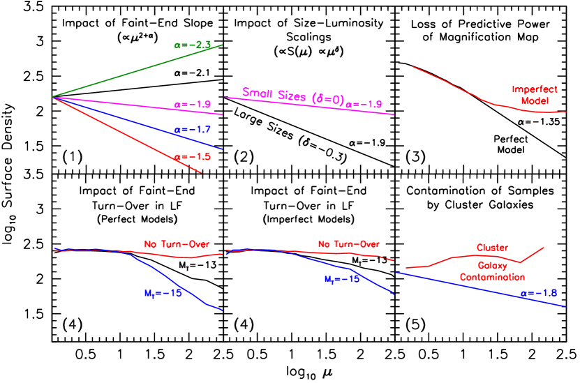
Figure 10.— Schematic illustrating how the surface density $\Sigma$ of galaxies would be expected to depend on the magnification factor $\mu$, as outlined in the five subsections of §4.1: the relevant subsection number is indicated in each panel. Five of the six panels illustrate a different issue that impacts the dependence. As shown in §3 of Bouwens et al. (2017: see also Broadhurst 1995, Broadhurst et al. 2005), the observed surface densities is expected to vary as $\mu^{2+\alpha}S(\mu)$ where $S(\mu)$ is the completeness of faint selections as a function of magnifications $\mu$. The numbering here and in the figure corresponds to the numbering in §4.1. (1) The upper left panel shows the expected dependence on the faint-end slope $\alpha$ of the LF (with assumed $\alpha$’s indicated on the figure), while (2) the upper middle panel shows the expected dependence on different size-luminosity relations, while keeping the assumed faint-end slope $\alpha$ fixed to $-$1.9. Different size-luminosity relations translate into different magnification-dependent selection efficiencies $S(\mu)$ which we model as $\mu^{\delta}$. The large size-luminosity relation shown here relies on the $S(\mu)\propto\mu^{-0.3}$ dependence found by Oesch et al. (2015), i.e., equivalent to $\delta=-0.3$ in the chosen parameterization, while the small size-luminosity relation assumes that sources are unresolved (e.g., Bouwens et al. 2017a; Kawamata et al. 2018; Bouwens et al. 2021b, 2022), resulting in a magnification-independent selection efficiency, i.e., $\delta=0$. (3) The upper right panel shows the expected flattening to the $\Sigma$ vs. model $\mu$ relationship, due to a breakdown in the predictive power of the models (see Figure 5 of Bouwens et al. 2017b where this result was previously shown) and assumes a faint-end slope of $-1.35$ to the $UV$ LF. (4) The lower left and center panels presents the impact of a turn-over in the $UV$ LF at the faint end, with no faint-end turn-over (red), a turn-over $M_{T}$ at $-15$ mag (black), and a turn-over $M_{T}$ at $-13$ mag (blue), respectively. The lower left panel shows the dependence assuming perfect recovery of the magnification factor, while the lower center panel shows the dependence in a more realistic scenario where the magnifications are uncertain. (5) The lower right panel contrasts the expected dependence for $z\sim 5$ galaxies (assuming a faint-end slope $\alpha$ of $-1.8$) with that expected including large numbers of foreground galaxies from the clusters Abell 2744 and MACS0416. The selection efficiency is assumed to be independent of magnification, i.e., $\delta=0$, except in the upper center panel.

4.1. Expected Dependencies on the Source Magnification Factor

There are at least five distinct effects which can impact the observed surface density of galaxies vs. magnification factor $\mu$. Each of these effects is illustrated in Figure 10 and discussed in the paragraphs that follow:

(1) Dependence on the Faint-end Slope $\alpha$: As we demonstrated earlier, it is well established (e.g. Broadhurst 1995) that the surface density of sources in our high-redshift samples scale as $\mu^{-(2+\alpha)}$ (e.g., Broadhurst 1995) assuming a Schechter form for the $UV$ LF. For this first case, we assume that source detectability does not depend on the magnification factor. Also assumed is that the model magnification factor is exactly equal to the true magnification factor everywhere.

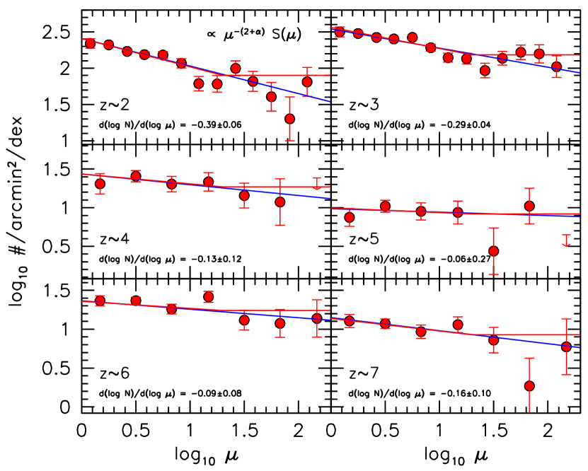
Figure 11.— The surface density of star-forming galaxies in our $z\sim 2$, $z\sim 3$, $z\sim 4$, $z\sim 5$, $z\sim 6$ and $z\sim 7$ selections (each shown in their own panel) vs. the median magnification factor from the parametric lensing models. The surface density is plotted per unit magnification factor (dex). The blue and red lines represent power-law fits to the binned red points, assuming a break-down in the predictive power of the lensing models at values greater than 300 and 30, respectively, i.e., $\mu_{break}=300$ and 30. As shown in §3 of Bouwens et al. (2017b), we would expect the observed surface densities to vary as $\mu^{-(2+\alpha)}S(\mu)$ where $S(\mu)$ is the completeness of faint selections as a function of magnifications $\mu$. As discussed in §4.2 and §4.3 and as shown in Figure 12, we see that such expectations are, in fact, realized, and there is a connection between the slopes of the lines plotted here and the best estimate faint-end slopes $\alpha$ observed in field studies.

For faint-end slopes $\alpha$ steeper than $-2$, the surface density of sources should be the highest in the highest magnification regions. For faint-end slopes of $-2$, the surface density of sources is independent of the magnification factor $\mu$. For faint-end slopes shallower than $-2$, the surface density of sources is highest in the lowest magnification regions. The upper-left panel of Figure 10 illustrates this expected dependencies, with faint-end slopes $\alpha$ of $-1.5$ (red line), $-1.7$ (blue line), $-1.9$ (magenta line), $-2.1$ (black line), and $-2.3$ (green line). The sensitivity of the results to the faint-end slope $\alpha$ is quite strong.

(2) Sizes and Surface Brightnesses of Lower-Luminosity Galaxies: In practice, the surface density we measure of lensed galaxies behind a cluster depends on their detection efficiency, which in turn can depend on the sizes or surface brightnesses of galaxies. For extended sources, Oesch et al. (2015) demonstrated that the detection efficiency $S(\mu)$ could show a noteworthy dependence on the magnification factor $\mu$, finding approximately an $\mu^{-0.3}$ dependence (e.g., as seen in Figure 3 of Oesch et al. 2015) for a model where the sizes are proportional to the luminosity $L$ to the 0.22 power (i.e., $L^{0.22}$). Bouwens et al. (2017a), Bouwens et al. (2017c), Kawamata et al. (2018), Bouwens et al. (2021b), and Bouwens et al. (2022) have argued that high-redshift sources at very low luminosities are very compact. If this is in fact the case, we would expect the detection efficiency of sources to show only a marginal dependence on the magnification factor $\mu$ and to depend only on the redshift and apparent magnitude of sources.

Incorporating the impact of the selection efficiency, we expect the surface densities to depend on the magnification factor $\mu$ as $\mu^{-(2+\alpha)}S(\mu)$. The upper-middle panel of Figure 10 illustrates the expected dependence of the surface densities on the magnification factor $\mu$ for especially compact sources where $S(\mu)\propto\mu^{0}$ (magenta line) and extended sources, such as Oesch et al. (2015) assumed in their simulations, where $S(\mu)\propto\mu^{-0.3}$ (black line). A faint-end slope $\alpha$ of $-1.9$ is assumed in both cases.

(3) Breakdown in Predictive Power of Lensing Models at high magnification factors $\mu$: Another important effect regards differences between the “true” magnification factors and model magnification factors. Given that the observed surface densities depend on the “true” magnification factors and not the model magnification factors, any breakdown in the relationship between the true and model magnification factors would impact the dependence the surface densities show on the estimated magnification factors.

Such a breakdown is expected to occur at magnification factors in excess of 50 to 100, as we for example show in Figures 5-7 (see also Meneghetti et al. 2017; Bouwens et al. 2017b). This effect would cause any dependence of surface density on the model magnification factor to be effectively washed out, resulting in galaxy surface densities asymptoting to a fixed value.

We illustrate such a breakdown in the dependence of the measured surface densities on the model magnification factor with the red line in the upper-right panel of Figure 10. If no such breakdown occurs and the model magnification maps can be effectively used to magnification factors of 300, the dependence would look like the black line in that panel. For this particular example, we adopt the results shown in the center panel of Figure 5 of Bouwens et al. (2017b), where the underlying model LF is assumed to have a faint-end slope $\alpha$ of $-1.35$, the observations are set up using the GLAFIC magnification models, and the recovered magnifications are from the CATS magnification models.

One consequence of this is for the recovered $UV$ LF to asymptote to a faint-end slope of $-2$ for a magnification-independent selection efficiency and $-2+d(\ln S(\mu))/d(\ln\mu)$ in the more general case (Appendix C of Bouwens et al. 2017b).

(4) Faint-end Turn-over in the $UV$ LF: A turnover in the UV LF at the faint end also impacts the dependence of source surface density on the magnification factor. Such a turn-over primarily impacts the number of sources found in the highest magnification regions probing the faintest sources and thus shows up as a decrease in the surface density of sources at high magnification factors.

As an illustration of the dependence expected, the predicted dependence on magnification factor is shown in Figure 10 (lower left and lower center panels) for $UV$ LFs with no faint-end turn-over and turn-overs at $-15$ mag and $-13$ mag. We implemented these turn-overs using the functional form earlier presented in Bouwens et al. (2017b), assuming the CATS v4.1 magnification model, and assuming perfect recovery of the magnification factors from the model in one case (lower left panel) and a more realistic recovery in a second case (lower center panel) using a median of the parametric models not including CATS. As is clear from the panels, the LFs with a faint-end turn-over show a break in the surface densities toward lower values at magnification factors higher than 15. In the cases where the magnification is uncertain (lower center panel), the influence of the turn-over on the surface density of galaxies at high magnifications is less obvious. Interested readers may also want to consult an earlier discussion on this topic by Leung et al. (2018).

(5) Contamination of $z\gtrsim 2$ Selections with Cluster Galaxies: The measured surface densities of $z\gtrsim 2$ selections vs. magnification factor can also be impacted if foreground galaxies significantly contaminate selections. While essentially all selections suffer from low levels of contamination, contamination can become much more serious when search fields have large numbers of foreground cluster galaxies that show Balmer or 4000Å breaks across exactly the same passbands as the Lyman-break in a given search (e.g., see Figure 3). For the HFF clusters, this can be a serious concern for $z\sim 4$ and $z\sim 5$ selections depending on the cluster redshift (see Figure 3).

Table 5Dependence of the Source Surface Density on the Magnification Factors and the Direct Implications

Redshift	Measured	Inferred
Sample	$\epsilon$	$\alpha$
Assuming Lensing Model Predictive Power $\mu_{break}=300$, $\delta=0$
z$\sim 2$	$-$0.38$\pm$0.05	$-$1.62$\pm$0.05
z$\sim 3$	$-$0.26$\pm$0.04	$-$1.74$\pm$0.04
z$\sim 4$	$-$0.14$\pm$0.14	$-$1.86$\pm$0.14
z$\sim 5$	$-$0.05$\pm$0.14	$-$1.95$\pm$0.14
z$\sim 6$	$-$0.12$\pm$0.08	$-$1.88$\pm$0.08
z$\sim 7$	$-$0.17$\pm$0.11	$-$1.83$\pm$0.11
Assuming Lensing Model Predictive Power $\mu_{break}=30$, $\delta=0$
z$\sim 2$	$-$0.39$\pm$0.06	$-$1.61$\pm$0.06
z$\sim 3$	$-$0.29$\pm$0.04	$-$1.71$\pm$0.04
z$\sim 4$	$-$0.13$\pm$0.15	$-$1.87$\pm$0.15
z$\sim 5$	$-$0.06$\pm$0.16	$-$1.94$\pm$0.16
z$\sim 6$	$-$0.10$\pm$0.09	$-$1.90$\pm$0.09
z$\sim 7$	$-$0.16$\pm$0.12	$-$1.84$\pm$0.12

Any significant contamination of our high-redshift samples by cluster galaxies would impact the surface density vs. magnification $\mu$ relation. The surface density of cluster galaxies is much higher towards the center of a cluster where the magnifications are higher than it is towards the outer parts of a cluster. If cluster galaxies substantially contaminated a selection, one would expect the surface density of galaxies to rise appeciably to magnification factors of 10 and perhaps flatten beyond that.

To provide an approximate illustration of what the impact of such contamination would be, we have created a selection of predominantly foreground sources from two HFF clusters, Abell 2744 and MACS0416, by determining the $V_{606}-Y_{105}$ vs. $J_{125}$ color magnitude relation for cluster galaxies and then including sources which lie within $|\Delta(V_{606}-Y_{105})|<0.2$ mag of the relation. Nominal magnification factors are then calculated for sources as if they were $z\sim 5$ galaxies, sources are segregated into different magnification bins, and then the surface density of these sources is derived as a function of the nominal magnification factor. The result is presented in the lower right panel of Figure 10 as the red line. While this selection likely includes a small number of distant sources, the slope and shape reflects the impact of contaminating cluster galaxies.

Clearly, the surface density vs. magnification relationship is different from the behavior from LFs with a relatively shallow faint-end slope, e.g., $\gtrsim-1.8$, where the surface density of sources decreases towards higher magnification factors. If contaminants are not eliminated from the intermediate and high-redshift samples, it could have a substantial impact on the recovered LF results using lensing clusters.

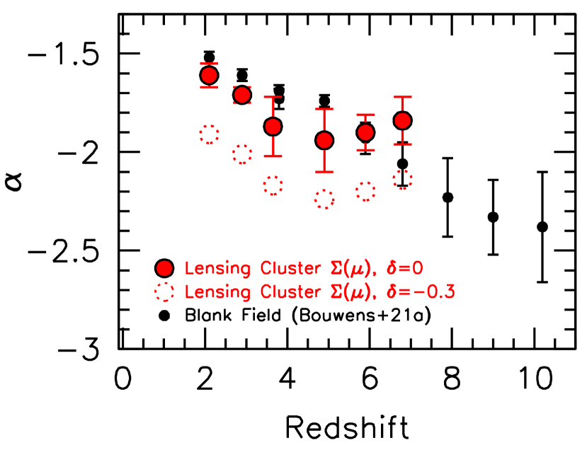
Figure 12.— Determinations of the faint-end slope $\alpha$ vs. redshift (red filled circles) from our HFF surface density analysis (§4.2 and §4.3) and a comparison to blank-field faint end slope determinations (black filled circles: Bouwens et al. 2021a). Error bars are $1\sigma$. The HFF faint-end slope results are derived based on the relationship between the observed galaxy surface densities and the magnification factors and assume that the selection volumes do not depend on the magnification factor, i.e., $\delta=0$ (as defined in Eq. 3); see §4.3. Also shown are the inferred faint-end slopes $\alpha$ assuming a magnification-dependent selection efficiency $\mu^{-0.3}$, i.e., with $\delta=-0.3$ (open dotted red circles). Amazingly, the results we obtain based on the magnification-dependent surface densities – assuming that $S(\mu)$ is independent of the magnification factor $\mu$, i.e., $\delta=0$ – are consistent with blank-field determinations.

In the above paragraphs, we discuss at least five different factors which can impact the measured surface density of sources vs. magnification factor. For some of the described factors, the impact is similar (e.g., faint-end slope $\alpha$ vs. sizes of faint sources), so some degeneracies can arise in interpreting the results.

Nevertheless, it is useful for us to construct a fiducial functional form for interpreting the surface density vs. magnification results. Based on previous work by Broadhurst (1995), Broadhurst et al. (2005), and Bouwens et al. (2017b) and also by the earlier discussion in this section, the surface density of galaxies in $z\gtrsim 2$ selections can be written as $\mu^{-(2+\alpha)}S(\mu)$. If we rewrite $S(\mu)$ as a power law with $\mu^{\delta}$, where the exponent $\delta$ expresses the dependence of the selection efficiency on the magnification factor:

$$\Sigma(\mu)=\mu^{-(2+\alpha)}\mu^{\delta}=\mu^{\epsilon}$$ (2)

where we set $\epsilon$ equal to $\delta-(2+\alpha)$ for simplicity.

As an approximate accounting for the expected predictive power of the model magnification factors above some value $\mu_{break}$ (upper right panel in Figure 10) – which is not well established, but seems likely to be anywhere from $\mu\sim 10$ to $\gtrsim$100 – we can replace $\mu$ with $\textrm{min}[\mu,\mu_{break}]$ in the above expression. This results in our recasting Eq. 2 as follows:

$$\Sigma(\mu)=(\textrm{min}[\mu,\mu_{break}])^{\epsilon}=(\textrm{min}[\mu,\mu_{break}])^{\delta-(2+\alpha)}$$ (3)

Given the challenges uncertainties in the magnification model pose to characterizing a potential turn-over at lower luminosities (e.g., see Bouwens et al. 2017b, Atek et al. 2018) and given that the impact of one runs counter to the other (lower center panel of Figure 10), we will largely ignore the issue of a faint-end turn-over for the results we derive in the following sections. This issue will nevertheless be revisited in the companion paper to the present one (R. Bouwens et al. 2022, in prep).

4.2. Observed Dependence of the Source Surface Densities on the Model Magnification Factors

Having discussed the expected dependencies on the model magnification factors, we now proceed to characterize how the surface density of galaxies in our $z\sim 2$-7 selections exhibit the expected traits. We focus on the selections for $z\sim 2$-7 galaxies because of the much larger number of sources in those selections. The $z\sim 8$, 9, and 10 samples are too small to map out the trends.

Using the median magnification factor we derive from the parametric model, we segregate the sources in each of our samples into different magnification bins, compute the total area available over all six HFF clusters to identify sources in a given bin of magnification (of width 0.166 and 0.333 dex for our $z\sim 2$-3 and $z\sim 4$-7 selections, respectively), and then derive the resultant surface densities. We present our results in Figure 11.

We model the surface densities as a simple power law in the magnification factor $\mu$, i.e., $\mu^{\epsilon}$, with a break in the power-law at $\mu_{break}=30$ and $\mu_{break}=300$. In the former case, we suppose that the model magnification factors retain their predictive power to 30 and in the latter case to 300. We include the latter case to show the behavior in the case that the models have predictive power beyond values of 30 (as suggested by our earlier results though it seems unlikely results would be predictive to values of 300). In the two cases, we find similar power-law slopes. The best-fit $\epsilon$’s derived from our power-law fits are presented in Table 5 and range from $-0.41$ to 0.02.

In the subsections which follow, we will attempt to interpret the observed trends to derive constraints on the faint-end slope $\alpha$ of the $UV$ LF at $z=2$-7, the dependence of selection efficiency $S(\mu)$ on the magnification factor (i.e., $\mu^{\delta}$), and the maximum magnification factor to which the lensing models are predictive.

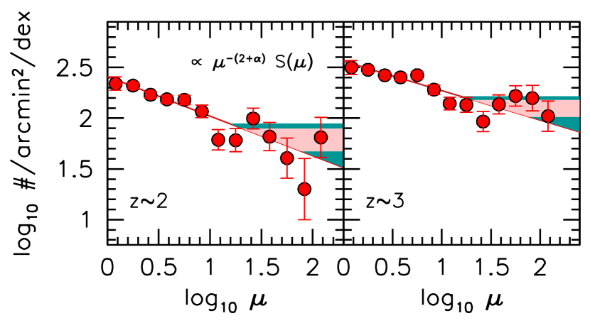
Figure 13.— Fits to the surface density vs. magnification relation for our $z\sim 2$ (left panel) and $z\sim 3$ samples (right panel: see §4.5). Shown with the shaded red and green contours are the 68% and 95% confidence constraints on the relation. As the upper right panel of Figure 10 illustrates, we would expect the surface density vs. magnification trend to maintain a linear form to the magnification factor where the models are predictive and then to flatten for even higher magnification factors. These fits suggest that the median of the parametric magnification models likely have predictive power to at least a magnification factor of 15 and 21 at 95% and 68% confidence, respectively. This provides a valuable independent test of the reliability of the v4 models to high magnification factors.

The challenge we face in attempting to address each of these questions is that our modeling, i.e., Eq (3), has more free parameters than constraints, and so some simplifying assumptions will need to be made.

4.3. Implications for the Selection Efficiencies

In our modeling surface density of galaxies as a function of the magnification $\mu$ using Eq. 3, we can simplify the situation considerably by setting the faint-end slope $\alpha$ in this equation equal to the faint-end slopes derived from extensive blank-field studies and then looking for the best-fit values of $\delta$ and $\mu_{break}$. Faint-end slopes from blank-field studies are increasingly well determined and should provide us with a well-defined reference point for our modeling. We take the blank-field slopes from the recent study of Bouwens et al. (2021a) who derive $z\sim 2$-9 LF results using a comprehensive set of blank-field data sets observed with HST.

The best-fit values of $\delta$ we derive in the $\mu=300$ and $\mu=30$ cases are 0.09${}_{-0.03}^{+0.04}$ and 0.08$\pm$0.04, respectively. This is very close to the case $\delta=0$, where the selection efficiency shows no dependence on the magnification factor of sources. Such a dependence is expected in the case of an especially steep size-luminosity relation for $z\sim 2$-9 galaxies, i.e., where $r\propto L^{0.5}$ and there is no change in the surface brightness of sources vs. luminosity or magnification factor at the faint end of the HFF probes. Interestingly enough, Bouwens et al. (2017a), Kawamata et al. (2018), Bouwens et al. (2022), and Yang et al. (2022) all found steep size-luminosity relations at $z\gtrsim 6$, with radius depending on luminosity as $L^{0.50\pm 0.07}$, $L^{0.46_{-0.09}^{+0.08}}$, $L^{0.40\pm 0.04}$, and $L^{0.48\pm 0.08}$.

As important context, a negative $\delta$ would be expected for the size-luminosity relations derived for brighter field galaxies in the intermediate or high-redshift universe. As one example, a $r\propto L^{0.27}$ relation, as derived by Shibuya et al. (2015) for $z=4$-8 galaxies, would result in the surface brightness of galaxies scaling as the square root of the luminosity. As a result, lower-luminosity lensed galaxy samples would feature very low surface brightness sources, resulting in a decrease in the selection efficiency of galaxies to higher magnification factors. Oesch et al. (2015) found $\delta\approx-0.3$ in the simulations they ran. Note that because gravitational lensing preserves the surface brightness of sources, lensing would have little impact in making low surface brightness galaxies more easily detectable.

Given the above considerations and our formal constraints on $\delta$, it appears that $\delta$ must be close to 0, and that a significant fraction of the lower luminosity $z=2$-9 galaxy population have very small rest-$UV$ sizes. One potential explanation for a potentially steeper size-luminosity relation in the rest-$UV$ is the possibility that only only a small part of a fainter star-forming galaxies may be experiencing prominent star formation at a time, resulting in a much smaller apparent physical size (Overzier et al. 2008; Ma et al. 2018; Ploeckinger et al. 2019; Bouwens et al. 2017c, 2021b, 2022).

The present conclusions are very similar to what we previously concluded from the tests we performed in Bouwens et al. (2017a) where we looked at the distribution of sources as a function of the shear factor $S$. This conclusion was bolstered by Bouwens et al. (2017a)’s results on the measured sizes of faint sources after stacking them along their major shear axes.

Taking $\delta$ to be equal to 0, we tabulate our determinations of the faint-end slope $\alpha$ of the $UV$ LF in Table 5. In Figure 12, we present these faint-end slope determinations vs. similar determinations of the faint-end slope $\alpha$ from the comprehensive field studies considered in the Bouwens et al. (2021a) analysis. The slopes shown in Figure 12 are for the $\mu_{break}=30$ case.

We can also see how different these faint-end slope determinations are from the case where the selection efficiency depended on the magnification factor to the $-0.3$ power, i.e., $\delta=-0.3$, as Oesch et al. (2015) found in the simulations they ran. If $\delta=-0.3$, we would derive faint-end slopes that were $\Delta\alpha\sim 0.3$ steeper than what we derived for our fiducial $\delta=0$ assumptions. As an illustration of the impact of such a change in $\delta$, we show, with the dotted open red circles in Figure 12, the faint-end slopes we derive assuming a $\delta=-0.3$. There is clearly significant tension between the $\delta=-0.3$ slopes and those derived from blank-field observations.

4.4. Predictive Power of Magnification Maps

As the upper-right panel of Figure 10 illustrates, the surface density $\Sigma$ vs. model magnification factor $\mu_{model}$ relation can significantly flatten at high magnification factors when the models lose their predictive power. This occurs due to different regions of the sky being unsuccessfully segregated in terms of their magnification levels, effectively resulting in a flat relation above some magnification factor.

As a result of this effect, through a careful modeling of the surface density vs. magnification factor relation, we can set constraints on the magnification factor to which the magnification models are predictive. Our strongest constraints come from our $z\sim 2$ and $z\sim 3$ samples, due to the steepness of the surface density vs. magnification relation in Figure 11 and significant statistics at $z\sim 2$ and $z\sim 3$. The steepness of the $z\sim 2$ and $z\sim 3$ relations can be readily contrasted with the flattening expected at high magnifications when the models lose their predictive power.

While redshifts $z\sim 2$ and $z\sim 3$ provide the strongest constraints, we make use of all of our $z\sim 2$-7 results and perform a simultaneous fit to the $\Sigma$ vs. $\mu_{model}$ relation to find the value of $\mu_{break}$ which yields the minimum value of $\chi^{2}$. We can then determine the range of $\mu_{break}$ which yield $\chi^{2}$’s consistent with the best-fit $\mu_{break}$. We find that $\mu_{break}$ is constrained to lie in the range 21 to 77 at 68% confidence and to be in excess of 15 at 95% confidence (Table 6). We illustrate the derived 68% and 95% confidence intervals on the $z\sim 2$ and $z\sim 3$ surface density vs. magnification relations in Figure 13 using the light red and cyan shadings, respectively.

As we discussed earlier, there have been efforts to test the predictive power of lensing model reconstruction efforts by Meneghetti et al. (2017). Meneghetti et al. (2017) produced a full set of mock observations for two galaxy clusters and obtained reconstructions of the lensing maps for these clusters based on the mock data sets. Encouragingly enough, Meneghetti et al. (2017) found that many of the blindly recovered magnification maps were reliable to magnification factors of at least 30. This is in excellent agreement with the results from this section and also earlier in this manuscript (Figures 5-7) using multiple independent models of the same cluster.

The constraints in this section, based on the surface density measurements, have significant utility in evaluating the public magnification models for the HFF clusters. They provide us with a highly independent assessment of both the quality and reliability of the magnification models.

Table 6New Constraints Obtained Modeling the $\Sigma$ vs. $\mu$ Relation

Parameter	Constraint
Magnification-Dependent Selection Efficiencies
$\delta$ ($\mu=300$)	0.09${}_{-0.03}^{+0.04}$
$\delta$ ($\mu=30$)	0.08$\pm$0.04
	$\approx$0
Predictive Power of Magnification Models
$\mu_{break}$	$<$15 (95% confidence)
	[21,77] (68% confidence)

4.5. Comparison to Previous Work on the Magnification Bias from the HFFs

Previously, Leung et al. (2018) made use of a deep selection of $z\geq 4.75$ galaxies behind the six HFF clusters to quantify the surface density of $z\geq 4.75$ galaxies vs. the magnification factor $\mu$. The surface density they derived for sources are highest in the regions with lower magnification factors and decrease by a factor of $\sim$5 to magnification factors of $>$50.

This is a slightly stronger dependence than what we find for galaxies in our $z\sim 4$, $z\sim 5$, and $z\sim 6$ samples, where we only observe a factor of $\sim$1-2$\times$ decrease in the surface densities from $\mu$ $\sim$1 to $\sim$50. It is unclear why Leung et al. (2018) find a stronger dependence than we do, but we note that they only consider those high magnification regions which show little contamination from intracluster light in the original images, and so only have a smaller sample to utilize.

Leung et al. (2018) interpret the steeper decline they find in the surface densities of $z\geq 4.75$ galaxies to high magnifications as providing evidence for a wave $\psi$ dark matter model (Schive et al. 2014) with boson masses spanning the range 0.8$\times$10^-22 eV to 3.2$\times$10^-22 eV. Such a dark matter scenario would favor a turn-over in the $UV$ LF somewhere between $-15$ and $-16.5$ mag.

While this is an exciting possibility, our surface density results do not show the same $\sim$5$\times$ decrease at magnification factors $\gtrsim$10 that Leung et al. (2018) find, as also illustrated in Figure 10. Therefore, at least according to our measurements, any turn-over in the $UV$ LF – if it exists – must occur at fainter luminosities than $-$16 mag. Independent constraints from Castellano et al. (2016), Livermore et al. (2017), Bouwens et al. (2017b), Ishigaki et al. (2018), and Atek et al. (2018) are also suggestive of the same conclusion, constraining a faint-end turn-over to occur at $\gtrsim$$-$15 mag.

5. Summary

In this paper, we have made use of the available HST observations over all six HFF cluster fields to assemble a comprehensive sample of 2534 lensed galaxies over the redshift range $z\sim 2$-9. Our samples include a total of 765 $z\sim 2$, 1176 $z\sim 3$, 274 $z\sim 6$, 125 $z\sim 7$, 51 $z\sim 8$, and 16 $z\sim 9$ galaxy candidates from the HFF cluster observations. In addition, 68 and 59 galaxy candidates are found at $z\sim 4$ and $z\sim 5$, respectively, using a much more conservative set of selection criteria (as required to minimize contamination from galaxies in the foreground clusters: see Figures 3 and 4). Including the two $z\sim 10$ candidates found by Oesch et al. (2018a), the cumulative sample of lensed $z=2$-10 galaxies includes 2536 distinct sources.

We estimate the luminosity of these sources by utilizing the median magnification factor from the latest (i.e., v3/v4) HFF lensing models (Table 2). These models make use of the comprehensive set of multiple image pairs available from the HFF observations, as well as a comprehensive set of spectroscopic redshift constraints.

By taking advantage of the availability of multiple independent models of each HFF cluster and alternatively treating one of the v4 parametric models as the truth, we assess how well the other models, considered both individually or as a median, are able to predict the magnification factors seen in the “true” model. We find that individual v4 magnification models are effective in predicting the magnification factors in other models to magnifications of $\sim$20-50 (Figure 5). When using the median magnification maps, the models are predictive to magnification factors of $\gtrsim$40 and in the case of Abell S1063, the predictive range appears to extend to magnification factors of $\sim$100.

We also assessed the robustness of the published magnification factors derived for different $z\sim 6$-10 samples from the literature (Zitrin et al. 2014; Infante et al. 2015; Livermore et al. 2017; Ishigaki et al. 2018). Using the median magnification factors from the v4 parametric models, we found that published magnification factors showed a significant degree of robustness. For magnification factors in excess of 50 and especially 100, the robustness of published magnification factors was less, with new estimates typically in the range 40 to 100.

Our tests cast doubt on the robustness of any magnification estimates in excess of 100, and therefore we take 100 as the maximum fiducial magnification factor. Imposing this magnification limit, the lowest luminosity galaxies that we identify behind the HFF clusters have $UV$ luminosities of $-$12.4 mag (at $z\sim 3$) and $-$12.9 mag (at $z\sim 7$).

We have made use of these large $z\sim 2$-9 samples of magnified galaxies to characterize the dependence of the surface densities on the magnification factors. Examining this relationship is particularly valuable, since this dependence not only provide us with constraints on the faint-end slope of the LF, and any possible turnover, but also gives us insight into the sizes of faint $z\geq 2$ galaxies and the predictive power of the lensing models.

We find the slope of the surface density vs. magnification relation is exactly what we would expect if the selection efficiencies showed no strong dependence on the magnification factor $\mu$. This can only be the case if lower luminosity sources are small, as concluded in Bouwens et al. (2017a, 2021b, 2022) and Kawamata et al. (2018). In the limit of no dependence of the selection efficiency on the magnification factor, we derive the faint-end slope of the LFs at $z\sim 2$, 3, 4, 5, 6, and 7. Excellent agreement is found with faint-end slope determinations from blank field studies (e.g., Bouwens et al. 2021a). This consistency strongly supports the conclusions we draw from the surface density vs. magnification results.

In addition, we use the strong systematic dependence of source surface density on magnification factor to constrain the predictive power of magnification models. If the magnification models are not accurate above a given magnification factor, one would expect the dependence to immediately flatten above that magnification factor. Our results indicate that the median magnification factors from the parametric models provide reliable results to at least a magnification factor of 21 and 15 (68 and 95% confidence, respectively).

In a companion paper (R. Bouwens et al. 2022, in prep) to the present analysis, we will be using the current selection of 2534 $z\sim 2$-9 galaxies to set constraints on the faint end form of the $UV$ LFs at $z=2$-9. This will include a careful characterization not only of how the faint-end slope of the $UV$ LF evolves from $z\sim 9$ to $z\sim 2$, but also to set limits on possible faint-end turn-overs to these same $UV$ LFs.

References

- Anders et al. (2003) Anders, P., & Fritze-v. Alvensleben, U. 2003, A&A, 401, 1063
- Alavi et al. (2014) Alavi, A., Siana, B., Richard, J., et al. 2014, ApJ, 780, 143
- Alavi et al. (2016) Alavi, A., Siana, B., Richard, J., et al. 2016, ApJ, 832, 56
- Atek et al. (2014) Atek, H., Richard, J., Kneib, J.-P., et al. 2014, ApJ, 786, 60
- Atek et al. (2015) Atek, H., Richard, J., Kneib, J.-P., et al. 2015a, ApJ, 800, 18
- Atek et al. (2015) Atek, H., Richard, J., Jauzac, M., et al. 2015b, ApJ, 814, 69
- Atek et al. (2018) Atek, H., Richard, J., Kneib, J.-P., & Schaerer, D. 2018, MNRAS, 479, 5184
- Beckwith et al. (2006) Beckwith, S. V. W., Stiavelli, M., Koekemoer, A. M., et al. 2006, AJ, 132, 1729
- Bertin and Arnouts (1996) Bertin, E. and Arnouts, S. 1996, A&AS, 117, 39
- Bhatawdekar et al. (2019) Bhatawdekar, R., Conselice, C. J., Margalef-Bentabol, B., et al. 2019, MNRAS, 486, 3805
- Binney et al. (1987) Binney, J., & Tremaine, S. 1987, Galactic Dynamics, Princeton University Press
- Bouwens et al. (2011) Bouwens, R. J., Illingworth, G. D., Oesch, P. A., et al. 2011, ApJ, 737, 90
- Bouwens et al. (2015) Bouwens, R. J., Illingworth, G. D., Oesch, P. A., et al. 2015, ApJ, 803, 34
- Bouwens et al. (2017) Bouwens, R. J., Illingworth, G. D., Oesch, P. A., et al. 2017a, ApJ, 843, 41
- Bouwens et al. (2017) Bouwens, R. J., Oesch, P. A., Illingworth, G. D., Ellis, R. S., & Stefanon, M. 2017b, ApJ, 843, 129
- Bouwens et al. (2017) Bouwens, R. J., Illingworth, G. D., Oesch, P. A., et al. 2017c, arXiv:1711.02090
- Bouwens et al. (2021) Bouwens, R. J., Oesch, P.A., Stefanon, M., et al. 2021a, AJ, 162, 47
- Bouwens et al. (2021) Bouwens, R. J., Illingworth, G. D., van Dokkum, P. G., et al. 2021b, AJ, 162, 255
- Bouwens et al. (2022) Bouwens, R. J., Illingworth, G. D., van Dokkum, P. G., et al. 2022, ApJ, 927, 81
- Boylan-Kolchin et al. (2015) Boylan-Kolchin, M., Weisz, D. R., Johnson, B. D., et al. 2015, MNRAS, 453, 1503
- Bradač et al. (2009) Bradač, M., Treu, T., Applegate, D., et al. 2009, ApJ, 706, 1201
- Brammer et al. (2008) Brammer, G. B., van Dokkum, P. G., & Coppi, P. 2008, ApJ, 686, 1503
- Broadhurst (1995) Broadhurst, T. 1995, astro-ph/9511150
- Broadhurst et al. (2005) Broadhurst, T., Takada, M., Umetsu, K., et al. 2005, ApJ, 619, L143
- Bruzual et al. (2003) Bruzual, G., & Charlot, S. 2003, MNRAS, 344, 1000
- Bunker et al. (2004) Bunker, A. J., Stanway, E. R., Ellis, R. S., & McMahon, R. G. 2004, MNRAS, 355, 374
- Burgasser et al. (2004) Burgasser, A. J., McElwain, M. W., Kirkpatrick, J. D., et al. 2004, AJ, 127, 2856
- Caminha et al. (2016) Caminha, G. B., Grillo, C., Rosati, P., et al. 2016, A&A, 587, A80
- Caminha et al. (2017) Caminha, G. B., Grillo, C., Rosati, P., et al. 2017, A&A, 600, A90
- Castellano et al. (2016) Castellano, M., Yue, B., Ferrara, A., et al. 2016b, ApJ, 823, L40
- Coe et al. (2015) Coe, D., Bradley, L., & Zitrin, A. 2015, ApJ, 800, 84
- Coleman et al. (1980) Coleman, G. D., Wu, C.-C., & Weedman, D. W. 1980, ApJS, 43, 393
- Diego et al. (2005) Diego, J. M., Sandvik, H. B., Protopapas, P., et al. 2005, MNRAS, 362, 1247
- Diego et al. (2007) Diego, J. M., Tegmark, M., Protopapas, P., & Sandvik, H. B. 2007, MNRAS, 375, 958
- Diego et al. (2015) Diego, J. M., Broadhurst, T., Molnar, S. M., Lam, D., & Lim, J. 2015a, MNRAS, 447, 3130
- Diego et al. (2015) Diego, J. M., Broadhurst, T., Zitrin, A., et al. 2015b, MNRAS, 451, 3920
- Diego et al. (2018) Diego, J. M., Schmidt, K. B., Broadhurst, T., et al. 2018, MNRAS, 473, 4279
- Dressel et al. (2012) Dressel, L., et al. 2012. “Wide Field Camera 3 Instrument Handbook, Version 5.0” (Baltimore: STScI)
- Illingworth et al. (2013) Illingworth, G. D., Magee, D., Oesch, P. A., et al. 2013, ApJS, 209, 6
- Infante et al. (2015) Infante, L., Zheng, W., Laporte, N., et al. 2015, ApJ, 815, 18
- Ishigaki et al. (2018) Ishigaki, M., Kawamata, R., Ouchi, M., et al. 2018, ApJ, 854, 73
- Jullo et al. (2009) Jullo, E., & Kneib, J.-P. 2009, MNRAS, 395, 1319
- Kawamata et al. (2016) Kawamata, R., Oguri, M., Ishigaki, M., Shimasaku, K., & Ouchi, M. 2016, ApJ, 819, 114
- Kawamata et al. (2018) Kawamata, R., Ishigaki, M., Shimasaku, K., et al. 2018, ApJ, 855, 4
- Keeton (2010) Keeton, C. R. 2010, General Relativity and Gravitation, 42, 2151
- Koekemoer et al. (2013) Koekemoer, A. M., Ellis, R. S., McLure, R. J., et al. 2013, ApJS, 209, 3
- Koekemoer et al. (2014) Koekemoer, A. M., Avila, R. J., Hammer, D., et al. 2014, American Astronomical Society Meeting Abstracts #223
- Kotulla et al. (2009) Kotulla, R., Fritze, U., Weilbacher, P., & Anders, P. 2009, MNRAS, 396, 462
- Kron (1980) Kron, R. G. 1980, ApJS, 43, 305
- Kuhlen & Faucher-Giguère (2012) Kuhlen, M., & Faucher-Giguère, C.-A. 2012, MNRAS, 423, 862
- Labbé et al. (2010) Labbé, I., González, V., Bouwens, R. J., et al. 2010a, ApJ, 708, L26
- Labbé et al. (2010) Labbé, I., González, V., Bouwens, R. J., et al. 2010b, ApJ, 716, L103
- Labbé et al. (2013) Labbé, I., Oesch, P. A., Bouwens, R. J., et al. 2013, ApJ, 777, L19
- Labbé et al. (2015) Labbé, I., Oesch, P. A., Illingworth, G. D., et al. 2015, ApJS, 221, 23
- Laporte et al. (2016) Laporte, N., Infante, L., Troncoso Iribarren, P., et al. 2016, ApJ, 820, 98
- Leung et al. (2018) Leung, E., Broadhurst, T., Lim, J., et al. 2018, ApJ, 862, 156
- Liesenborgs et al. (2006) Liesenborgs, J., De Rijcke, S., & Dejonghe, H. 2006, MNRAS, 367, 1209
- Limousin et al. (2016) Limousin, M., Richard, J., Jullo, E., et al. 2016, A&A, 588, A99
- Livermore et al. (2017) Livermore, R., Finkelstein, S., Lotz, J. 2017, ApJ, 835, 113
- Lotz et al. (2017) Lotz, J. M., Koekemoer, A., Coe, D., et al. 2017, ApJ, 837, 97
- Ma et al. (2018) Ma, X., Hopkins, P. F., Boylan-Kolchin, M., et al. 2018, MNRAS, 477, 219
- Mahler et al. (2018) Mahler, G., Richard, J., Clément, B., et al. 2018, MNRAS, 473, 663
- Meneghetti et al. (2017) Meneghetti, M., Natarajan, P., Coe, D., et al. 2017, MNRAS, 472, 3177
- Merlin et al. (2016) Merlin, E., Amorín, R., Castellano, M., et al. 2016, A&A, 590, A30
- Merten et al. (2015) Merten, J., Meneghetti, M., Postman, M., et al. 2015, ApJ, 806, 4
- Oesch et al. (2015) Oesch, P. A., Bouwens, R. J., Illingworth, G. D., et al. 2015, ApJ, 808, 104
- Oesch et al. (2018) Oesch, P. A., Bouwens, R. J., Illingworth, G. D., Labbé, I., & Stefanon, M. 2018a, ApJ, 855, 105
- Oesch et al. (2018) Oesch, P. A., Montes, M., Reddy, N., et al. 2018b, ApJS, 237, 12
- Oguri (2010) Oguri, M. 2010, PASJ, 62, 1017
- Oke & Gunn (1983) Oke, J. B., & Gunn, J. E. 1983, ApJ, 266, 713
- Overzier et al. (2008) Overzier, R. A., Heckman, T. M., Kauffmann, G., et al. 2008, ApJ, 677, 37
- Owers et al. (2011) Owers, M. S., Randall, S. W., Nulsen, P. E. J., et al. 2011, ApJ, 728, 27
- Peng et al. (2002) Peng, C. Y., Ho, L. C., Impey, C. D., & Rix, H.-W. 2002, AJ, 124, 266
- Peng et al. (2010) Peng, C. Y., Ho, L. C., Impey, C. D., & Rix, H.-W. 2010, AJ, 139, 2097
- Ploeckinger et al. (2019) Ploeckinger, S., Schaye, J., Hacar, A., et al. 2019, MNRAS, 484, 4379
- Priewe et al. (2017) Priewe, J., Williams, L. L. R., Liesenborgs, J., et al. 2017, MNRAS, 465, 1030
- Richard et al. (2014) Richard, J., Jauzac, M., Limousin, M., et al. 2014, MNRAS, 444, 268
- Robertson et al. (2015) Robertson, B. E., Ellis, R. S., Furlanetto, S. R., & Dunlop, J. S. 2015, ApJ, 802, L19
- Schive et al. (2014) Schive, H.-Y., Chiueh, T., & Broadhurst, T. 2014, Nature Physics, 10, 496
- Schlafly & Finkbeiner (2011) Schlafly, E. F. & Finkbeiner, D. P. 2011, ApJ, 737, 103
- Schmidt et al. (2014) Schmidt, K.B., Treu, T., Brammer., G.B., et al. 2014, ApJ, 782, L36
- Sebesta et al. (2016) Sebesta, K., Williams, L. L. R., Mohammed, I., Saha, P., & Liesenborgs, J. 2016, MNRAS, 461, 2126
- Shibuya et al. (2015) Shibuya, T., Ouchi, M., & Harikane, Y. 2015, ApJS, 219, 15
- Shipley et al. (2018) Shipley, H. V., Lange-Vagle, D., Marchesini, D., et al. 2018, ApJS, 235, 14
- Szalay et al. (1999) Szalay, A. S., Connolly, A. J., & Szokoly, G. P. 1999, AJ, 117, 68
- Turner et al. (1984) Turner, E. L., Ostriker, J. P., & Gott, J. R. 1984, ApJ, 284, 1
- Umetsu & Broadhurst (2008) Umetsu, K., & Broadhurst, T. 2008, ApJ, 684, 177
- Vanzella et al. (2014) Vanzella, E., Fontana, A., Zitrin, A., et al. 2014, ApJ, 783, L12
- Weisz et al. (2014) Weisz, D. R., Johnson, B. D., & Conroy, C. 2014, ApJ, 794, L3
- Yang et al. (2022) Yang, L., Leethochawalit, N., Treu, T., et al. 2022, /mnras, submitted, arXiv:2201.08858
- Yue et al. (2018) Yue, B., Castellano, M., Ferrara, A., et al. 2018, ApJ, 868, 115
- Zheng et al. (2014) Zheng, W., Shu, X., Moustakas, J., et al. 2014, ApJ, 795, 93
- Zheng et al. (2017) Zheng, W., Zitrin, A., Infante, L., et al. 2017, ApJ, 836, 210
- Zitrin et al. (2012) Zitrin, A., Broadhurst, T., Bartelmann, M., et al. 2012, MNRAS, 423, 2308
- Zitrin et al. (2013) Zitrin, A., Meneghetti, M., Umetsu, K., et al. 2013, ApJ, 762, L30
- Zitrin et al. (2014) Zitrin, A., Zheng, W., Broadhurst, T., et al. 2014, ApJ, 793, L12
- Zitrin et al. (2015) Zitrin, A., Fabris, A., Merten, J., et al. 2015, ApJ, 801, 44