Joint Active and Passive Beamforming Design for IRS-Aided Radar-Communication

Abstract

In this paper, we study an intelligent reflecting surface (IRS)-aided radar-communication (Radcom) system, where the IRS is leveraged to help Radcom base station (BS) transmit the joint of communication signals and radar signals for serving communication users and tracking targets simultaneously. The objective of this paper is to minimize the total transmit power at the Radcom BS by jointly optimizing the active beamformers, including communication beamformers and radar beamformers, at the Radcom BS and the phase shifts at the IRS, subject to the minimum signal-to-interference-plus-noise ratio (SINR) required by communication users, the minimum SINR required by the radar, and the cross-correlation pattern design. In particular, we consider two cases, namely, case I and case II, based on the presence or absence of the radar cross-correlation design and the interference introduced by the IRS on the Radcom BS. For case I where the cross-correlation design and the interference are not considered, we prove that the dedicated radar signals are not needed, which significantly reduces implementation complexity and simplifies algorithm design. Then, a penalty-based algorithm is proposed to solve the resulting non-convex optimization problem. Whereas for case II considering the cross-correlation design and the interference, we unveil that the dedicated radar signals are needed in general to enhance the system performance. Since the resulting optimization problem is more challenging to solve as compared with the case I, the semidefinite relaxation (SDR) based alternating optimization (AO) algorithm is proposed. Particularly, instead of relying on the Gaussian randomization technique to obtain an approximate solution by reconstructing rank-one solution, the tightness is achieved by our proposed reconstruction strategy. Simulation results demonstrate the effectiveness of proposed algorithms and also show the superiority of the proposed scheme over various benchmark schemes.

I Introduction

The rapid increase of mobile data and Internet of Things (IoT) devices are creating unprecedented challenges for wireless service providers to provide high data rate and ultra-reliable low latency communication due to the limited frequency spectrum from $700~{}{\rm MHz}$ and $2.6~{}{\rm GHz}$ in the existing communication networks [1]. In contrast, the radar system has fruitful spectrum resource and typically operate ranging from $0.3{\text{-}}100~{}{\rm GHz}$, such as S band $(2{\text{-}}4~{}{\rm GHz})$, C band $(4{\text{-}}8~{}{\rm GHz})$, and X band $(8{\text{-}}12.5~{}{\rm GHz})$, depending on specific application requirements [2]. The coexistence (or spectrum sharing) design between the radar system and the wireless communication system is attracting great attention, which allows the communication system to use the spectrum resource of the radar system [3]. To mitigate the interference between the above two systems, several promising approaches are proposed, such as the opportunistic spectrum sharing approach [4], the null-space projection based approach [5, 6], and the joint design of radar waveform and communication beamforming [7, 8]. However, such separated deployment, i.e., the radar transceiver and the communication transmitter are geographically separated, requires additional information, such as the channel state information (CSI), radar probing waveforms, and communication modulation format, etc., to exchange to coordinate the simultaneous radar and communication transmissions, which significantly increases the complexity for hardware implementation in practice.

The radar-communication (Radcom) system (also known as the dual-function radar-communication system [9]), which integrates the radar and communication functions into a single hardware platform and is regarded as a promising solution to simplify the system design [10]. The RadCom system is able to simultaneously perform both radar and communication functionalities using the same signals transmitted from a fully-shared transmitter, which does not require to exchange information and naturally achieves full cooperation. In the early stage, the information is embedded into the radar pulses so that the communication transmission can be readily realized by using the already fabricated radar platforms. For example, the communication symbols embedding into radar pulses and/or sidelobe can be realized by controlling the radar pulse’s amplitude, phase shift, and even index modulation [11, 12, 13]. However, such approaches result in a low data rate for transmission since the transmission rate is fundamentally constrained by the radar pulse repetition frequency. Another important paradigm of research in existing works on Radcom is the transmit beamforming design [5, 14, 15]. Compared to the information embedding approaches, the transmit beamforming design potentially supports high data rate and guarantees radar performance by synthesizing a joint waveform that is shared by both radar and communications. The seminal work in [5] analyzed the synthesized waveform performance in the shared deployment system, and showed that the shared deployment significantly outperforms than the separated deployment in terms of the trade-off between the radar beampattern synthesis and the quality of communication. Instead of using the synthesized waveforms, the authors in [16] proposed to transmit the combination signals with communication beamformers and radar waveforms at the Radcom base station (BS), where the communication beamformers are used for serving communication users and radar waveforms are used for radar sensing, which provides more degrees of freedom for system design. The results in [16] showed that the communication-only beamformer design is inferior to the joint design of communication beamformer and radar waveform in terms of beampattern synthesis, especially when the number of communication users is less than the number of targets. The authors in [17] further answered whether radar waveforms are needed under different design criteria, channel conditions, and receiver types. However, the above works focused on either the beamforming/waveform design or encoding design, the limited degrees of freedom such as the uncontrollable of electromagnetic waves propagation still confine the system performance.

Recently, intelligent reflecting surfaces (IRSs) attract great attention both from industry and academia [18, 19, 20]. The IRS is composed of large numbers of passive and low-cost reflecting elements, each of which is able to independently adjust phase shift and/or amplitude on the impinging electromagnetic signals, so that it is able to controllably change the electromagnetic waves propagation towards any directions of interest. The seminal work in [21] unveiled the fundamental scaling law of the IRS by showing that the received signal-to-noise (SNR) is quadratically increasing with the number of IRS reflecting elements. Based on this appealing result, the IRS has been exploited for different applications such as wireless information transmission [22, 23, 24], wireless-powered communication network [25, 26, 27], unmanned aerial vehicle communication [28, 29, 30], and non-orthogonal multiple access [31, 32, 33], etc. To unleash the full potential of the Radcom system for both communication and radar sensing, the integration of IRS in the Radcom system is also ongoing. A handful of works, see e.g., [34, 35, 36, 37], studied the fundamental problem of target detection with the help of IRS in the radar-only system. Some further works, see, e.g., [38, 39, 40, 41], focused on the Radcom system by exploiting IRS to enhance the sensing performance while satisfying the quality-of-service (QoS) of users. The authors in [38] and [39] studied one communication user scenario. To be specific, work [38] studied one target sensing and aimed at maximizing the radar SNR while guaranteeing the QoS of the user by the joint optimization of IRS phase shifts and transmit covariance matrix. In [39], the authors studied the scenario where the BS and multiple sensing targets are blocked and constructed a virtual line-of-sight (LoS) link between the IRS and targets for target sensing. The authors in [40] and [41] further studied the joint design of the active beamforming and the passive beamforming for the multi-user scenario in RIS-assisted Radcom system. The minimization of multi-user interference under the predefined beampattern constraint was studied in [40]. The authors in [41] studied the scenario that the target sensing is corrupted by multiple clutters with the signal-dependent interference and aimed to maximize the radar SINR. However, the above works ignore the impact of interference introduced by the IRS and radar cross-correlation on the system. In addition, regarding the transceiver design for the joint waveform design or the single waveform design is also not answered and studied.

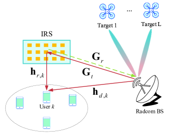
Figure 1: An IRS-aided Radcom system.

To address the above challenges, this paper studies an IRS-aided Radcom system in multi-user and multi-target scenarios as shown in Fig. 1. Based on the presence or absence of the radar cross-correlation design and the interference introduced by the IRS on the Radcom BS, two cases, namely, case I and case II, are studied. In particular, we answer the fundamental question: whether the dedicated radar signals are needed for these two cases? The main contributions of this paper are summarized as follows.

• We study an IRS-aided Radcom system, where the IRS is leveraged to help the Radcom BS transmit the joint of communication signals and radar signals for serving communication users and tracking targets. Our objective is to minimize the total transmit power at the Radcom BS by jointly optimizing the active beamformers at the Radcom BS and the phase shifts at the IRS, subject to the minimum signal-to-interference-plus-noise ratio (SINR) required by communication users, the minimum SINR required by the radar, and the cross-correlation pattern design. In particular, we consider two cases, i.e., case I and case II, based on the presence or absence of the radar cross-correlation design and the interference introduced by the IRS on the Radcom BS, which results in two different optimization problems.

• For case I where the interference introduced by the IRS is perfectly canceled and the cross-correlation design is ignored. Since the resulting optimization problem is non-convex, there are no standard convex methods to solve it optimally. To solve the problem, we first rigorously prove that the dedicated radar signals are not needed in this case, which significantly reduces implementation complexity and simplifies the following algorithm design. Then, we propose a novel penalty-based algorithm, which includes a two-layer iteration, i.e., an inner layer iteration and an outer layer iteration. The inner layer solves the penalized optimization problem, while the outer layer updates the penalty coefficient over iterations to guarantee convergence. In particular, the solution to each subproblem in the inner layer is solved by either a closed-form expression or a semi-closed-form expression.

• For case II where both the cross-correlation pattern design and the interference introduced by the IRS are considered. Since the resulting optimization problem is more challenging to solve than case I, the proposed penalty-based algorithm in case I cannot be applicable to this case. To solve this difficulty, a semidefinite relaxation (SDR)-based alternating optimization (AO) is proposed. In particular, instead of relying on the Gaussian randomization technique to obtain an approximation solution, the tightness is achieved by our proposed reconstruction strategy. In addition, we unveil that the dedicated radar signals are needed in general for this case to enhance the system performance.

• Our simulation results demonstrate that the IRS is beneficial for reducing the transmit power required by the Radcom BS in case I. In addition, it is shown that in case II, as the IRS is deployed far from the Radcom BS, the IRS is helpful for reducing transmit power, while as the IRS is deployed in the vicinity of the Radcom BS, the IRS may even deteriorate the system performance due to the interference. Furthermore, the results also show that adopting dedicated radar signals at the Radcom BS can significantly reduce the system outage probability as compared to the case without adopting the dedicated radar signals in case II.

The rest of this paper is organized as follows. Section II introduces the system model and problem formulation for the considered IRS-aided Radcom system. In Section III, a penalty-based algorithm is proposed to solve case I. In Section IV, an SDR-based AO algorithm is proposed to solve case II. Numerical results are provided in Section V and the paper is concluded in Section VI.

Notations: Boldface upper-case and lower-case letter denote matrix and vector, respectively. ${\mathbb{C}}^{d_{1}\times d_{2}}$ stands for the set of complex $d_{1}\times d_{2}$ matrices. For a scalar value $x$, ${\left|{x}\right|}$ represents the Euclidean norm of $x$. For a vector $\bf x$, ${\bf x}^{*}$ and ${\bf x}^{H}$ stand for its conjugate and conjugate transpose, respectively, and ${\rm diag}(\bf x)$ denotes a diagonal matrix whose main diagonal elements are extracted from vector $\bf x$. For a matrix $\bf X$, ${\rm{Tr}}\left({\bf{X}}\right)$ and ${\rm{rank}}\left({\bf{X}}\right)$ stand for its trace and rank, respectively, while ${\bf{X}}\succeq{\bf{0}}$ indicates that matrix $\bf X$ is positive semi-definite. A circularly symmetric complex Gaussian random vector $\bf x$ with mean $\bm{\mu}$ and covariance matrix ${\bf{\Sigma}}$ is denoted by ${\bf{x}}\sim{\cal CN}\left({\bm{\mu},{\bf{\Sigma}}}\right)$. ${\mathbb{E}}(\cdot)$ denotes the expectation operation. ${\cal O}\left(\cdot\right)$ is the big-O computational complexity notation.

II System Model and Problem Formulation

II-A System Model

Consider an IRS-aided Radcom system consisting of a Radcom BS, $K$ single-antenna users with the set denoted by ${\cal K}=\{1,\dots,K\}$, $L$ radar targets with the set denoted by ${\cal L}=\{1,\dots,L\}$, and an IRS with $M$ reflecting elements and with the set denoted by ${\cal M}=\{1,\dots,M\}$, as shown in Fig. 1. The Radcom BS is equipped with $N_{t}+N_{r}$ antennas, of which $N_{t}$ transmit antennas are used for serving communication users and tracking radar targets at the same time, while $N_{r}$ receive antennas are dedicated to receiving the echo signals reflected by radar targets.

II-A1 Transmit Waveform Design

The transmitted signal by the Radcom BS is given by

$${\bf{s}}={{\bf{W}}_{c}}{{\bf{x}}_{c}}+{{\bf{W}}_{r}}{{\bf{x}}_{r}},$$ (1)

where ${{\bf{x}}_{c}}\in{{\mathbb{C}}^{{K}\times 1}}$ denotes the transmit signals intended for communication users satisfying ${{\bf{x}}_{c}}\sim{\cal CN}\left({{\bf{0}},{{\bf{I}}_{K}}}\right)$ and ${{\bf{W}}_{c}}\in{{\mathbb{C}}^{{N_{t}}\times{K}}}$ represents the corresponding communication beamformer. Similarly, ${{\bf{x}}_{r}}\in{{\mathbb{C}}^{{N_{t}}\times 1}}$ denotes $N_{t}$ individual radar signals satisfying ${\mathbb{E}}\left\{{{{\bf{x}}_{r}}}\right\}={\bf{0}}_{N_{t}\times 1}$ and ${\mathbb{E}}\left\{{{{\bf{x}}_{r}}{\bf{x}}_{r}^{H}}\right\}={{\bf{I}}_{{N_{t}}}}$, and ${{\bf{W}}_{r}}\in{{\mathbb{C}}^{{N_{t}}\times{N_{t}}}}$ represents the radar beamformer. In addition, we assume that the communication and radar signals are statistically independent and uncorrelated, i.e., ${\mathbb{E}}\left\{{{{\bf{x}}_{c}}{\bf{x}}_{r}^{H}}\right\}={{\bf{0}}_{K\times{N_{t}}}}$ [16].

II-A2 Communication Model

We consider a quasi-static flat-fading channel in which the CSI remains unchanged in a channel coherence block, but may change in the subsequent blocks. We assume that the perfect CSI of all involved channels for communication is available at the Radcom BS via sending pilot signals by users [19]. Without loss of generality, in the downlink transmission, denote by ${\bf{G}}_{t}\in{{\mathbb{C}}^{M\times N_{t}}}$, ${\bf{h}}_{r,k}^{H}\in{{\mathbb{C}}^{1\times M}}$, and ${{\bf h}^{H}_{d,k}}\in{{\mathbb{C}}^{1\times N_{t}}}$ the complex equivalent baseband channel between the Radcom BS and the IRS, between the IRS and the $k$th user, and between the Radcom BS and the $k$th user, $k\in{\cal K}$, respectively. In addition, denote by ${\bf{G}}_{r}\in{{\mathbb{C}}^{N_{r}\times M}}$ the complex equivalent baseband channel between the Radcom BS and the IRS in the uplink transmission. The received signal by user $k$ in the downlink is given by

$${y_{k}}=\left({{\bf{h}}_{d,k}^{H}+{\bf{h}}_{r,k}^{H}{\bf{\Theta}}{{\bf{G}}_{t}}}\right){\bf{s}}+{n_{k}},$$ (2)

where ${\bf{\Theta}}={\rm{diag}}\left({{v_{1}},\cdots,{v_{M}}}\right)$ represents the IRS reflection coefficient matrix and $v_{m}$ denotes the phase shift corresponding to the $m$th IRS reflecting element with $\left|{{v_{m}}}\right|=1$, and $n_{k}\sim{\cal CN}\left({0,\sigma^{2}}\right)$ stands for the additive white Gaussian noise at user $k$. Define ${{\bf{W}}_{c}}=\left[{{{\bf{w}}_{c,1}},\ldots,{{\bf{w}}_{c,K}}}\right]$, where ${{\bf{w}}_{c,k}}\in{{\mathbb{C}}^{{N_{t}}\times 1}}$ denotes the $k$th column vector of ${{\bf{W}}_{c}},k\in{\cal K}$. Similarly, define ${{\bf{W}}_{r}}=\left[{{{\bf{w}}_{r,1}},\ldots,{{\bf{w}}_{r,{N_{t}}}}}\right]$, where ${{\bf{w}}_{r,i}}\in{{\mathbb{C}}^{{N_{t}}\times 1}}$ denotes the $i$th column vector of ${{\bf{W}}_{r}}$, $i\in{\cal N}_{t}=\{1,\dots,N_{t}\}$. As such, the received SINR by user $k$ is given by

$${\rm{SIN}}{{\rm{R}}_{k}}=\frac{{{{\left|{{\mathbf{h}}_{k}^{H}{{\mathbf{w}}_{c,k}}}\right|}^{2}}}}{{\sum\limits_{i\neq k}^{K}{{{\left|{{\mathbf{h}}_{k}^{H}{{\mathbf{w}}_{c,i}}}\right|}^{2}}+\sum\limits_{j=1}^{{N_{t}}}{{{\left|{{\mathbf{h}}_{k}^{H}{{\mathbf{w}}_{r,j}}}\right|}^{2}}}+{\sigma^{2}}}}},k\in{\cal K},$$ (3)

where ${\bf{h}}_{k}^{H}{\rm{=}}{\bf{h}}_{d,k}^{H}+{\bf{h}}_{r,k}^{H}{\bf{\Theta G}}_{t}$.

II-A3 Radar Model

Under the assumption that the propagation is nondispersive for tracking targets, the signal at the $l$th target location with angle $\theta_{l}$, $l\in{\cal L}$, can be described as ${\bf{a}}_{t}^{H}\left({{\theta_{l}}}\right){\bf{s}}$, where ${\bf{a}}_{t}^{H}\left(\theta\right)\in{{\mathbb{C}}^{1\times{N_{t}}}}=\left[{1,{e^{-j2\pi d\sin\left(\theta\right)/\lambda}},\ldots,{e^{-j2\pi d\left({{N_{t}}-1}\right)\sin\left(\theta\right)/\lambda}}}\right]$ stands for the transmit steering vector at direction $\theta$ with $d$ denoting the antenna spacing and $\lambda$ denoting the carrier wavelength. The received echo signals at the Radcom BS comes from four aspects, i.e., radar-target-radar channel, radar-IRS-radar channel, radar-IRS-target-radar channel, and radar-target-IRS-radar channel. However, [34] showed by both theoretical analysis and numerical simulations that the signals go through the radar-target-IRS-radar channel and radar-IRS-target-radar channel are highly attenuated due to three-hop transmissions, which has little impact on the system performance improvement. Thus, we only need to consider the former two types of echo signals and the received echo signals at the Radcom BS is given by

$${{\bf{y}}_{r}}=\underbrace{\sum\limits_{l=1}^{L}{{\beta_{l}}{{\bf{a}}_{r}}\left({{\theta_{l}}}\right){\bf{a}}_{t}^{H}\left({{\theta_{l}}}\right)}{\bf{s}}}_{{\rm{reflected{\kern 1.0pt}{\kern 1.0pt}by{\kern 1.0pt}{\kern 1.0pt}targets}}}+\underbrace{{{\bf{G}}_{r}}{\bf{\Theta}}{{\bf{G}}_{t}}{\bf{s}}}_{{\rm{reflected{\kern 1.0pt}{\kern 1.0pt}by{\kern 1.0pt}{\kern 1.0pt}the{\kern 1.0pt}{\kern 1.0pt}IRS}}}{\rm{+}}{{\bf n}_{r}},$$ (4)

where $\beta_{l}$ represents the reflection coefficient of the $l$th target, which is proportional to the radar-cross section (RCS) of the $l$th target and ${{\bf{n}}_{r}}\sim{\cal CN}\left({{\bf{0}},{{\sigma}^{2}}{{\bf{I}}_{{N_{r}}}}}\right)$ stands for the additive white Gaussian noise at the Radcom BS. In addition, similar to ${\bf{a}}_{t}^{H}\left(\theta\right)$, ${{\bf{a}}_{r}}\left(\theta\right)\in{{\mathbb{C}}^{{N_{r}}\times 1}}$ denotes the receive steering vector at direction $\theta$. Here, two key points need to be highlighted. First, the communication signals, i.e., ${{\bf{W}}_{c}}{{\bf{x}}_{c}}$, are not interference for target tracking in the Radcom system (in other words, the communication signals are not only used for downlink communication but also used for target tracking) since the communication signals are known at the Radcom BS. Second, since the reflected signals by IRS in (4) do not contain any information about the targets’ information, the radar SINR can be expressed as [8, 45]

$${\rm{SIN}}{{\rm{R}}_{r}}={\rm{tr}}\left({{\bf{AR}}{{\bf{A}}^{H}}{{\left({{\bf{BR}}{{\bf{B}}^{H}}+{\sigma^{2}}{{\bf{I}}_{{N_{r}}}}}\right)}^{-1}}}\right),$$ (5)

where ${\bf{R}}=\sum\limits_{k=1}^{K}{{{\bf{w}}_{c,k}}{\bf{w}}_{c,k}^{H}+}\sum\limits_{i=1}^{{N_{t}}}{{{\bf{w}}_{r,i}}{\bf{w}}_{r,i}^{H}}$, ${\mathbf{A}}{\text{ = }}\sum\limits_{l=1}^{L}{{\beta_{l}}{{\mathbf{a}}_{r}}\left({{\theta_{l}}}\right){\mathbf{a}}_{t}^{H}\left({{\theta_{l}}}\right)}$, and ${\bf{B}}={{\bf{G}}_{r}}{\bf{\Theta G}}_{t}$.

II-B Problem Formulation

The objective of this paper is to minimize the total transmit power at the Radcom BS by jointly optimizing the active beamformers at the Radcom BS and the phase shifts at the IRS, subject to the minimum SINR required by communication users, the minimum SINR required by radar, and cross-correlation pattern design. Accordingly, the optimization problem is formulated as

$$\mathop{\min}\limits_{{\{v_{m}\}},{\left\{{{{\bf{w}}_{c,i}}}\right\},\left\{{{{\bf{w}}_{r,i}}}\right\}}}\sum\limits_{k=1}^{K}{{{\left\|{{{\bf{w}}_{c,k}}}\right\|}^{2}}+}\sum\limits_{i=1}^{{N_{t}}}{{{\left\|{{{\bf{w}}_{r,i}}}\right\|}^{2}}}$$ (6a)

$${\rm s.t.}~{}\frac{{{{\left|{{\bf{h}}_{k}^{H}{{\bf{w}}_{c,k}}}\right|}^{2}}}}{{\sum\limits_{i\neq k}^{K}{{{\left|{{\bf{h}}_{k}^{H}{{\bf{w}}_{c,i}}}\right|}^{2}}+\sum\limits_{i=1}^{{N_{t}}}{\left|{{\bf{h}}_{k}^{H}{{\bf{w}}_{r,i}}}\right|}^{2}+{\sigma^{2}}}}}\geq{r_{k,{\rm{th}}}},k\in{\cal K},$$ (6b)

$$\qquad{\rm{tr}}\left({{\bf{AR}}{{\bf{A}}^{H}}{{\left({{\bf{BR}}{{\bf{B}}^{H}}+{\sigma^{2}}{{\bf{I}}_{{N_{r}}}}}\right)}^{-1}}}\right)\geq{r_{r,{\rm{th}}}},$$ (6c)

$$\qquad\sum\limits_{l=1}^{L-1}{\sum\limits_{j=l+1}^{L}{{{\left|{{\bf{a}}_{t}^{H}\left({{\theta_{l}}}\right)\left({\sum\limits_{k=1}^{K}{{{\bf{w}}_{c,k}}{\bf{w}}_{c,k}^{H}+}\sum\limits_{i=1}^{{N_{t}}}{{{\bf{w}}_{r,i}}{\bf{w}}_{r,i}^{H}}}\right){\bf{a}}_{t}\left({{\theta_{j}}}\right)}\right|}^{2}}}}\leq{\epsilon_{{\rm{th}}}},$$ (6d)

$$\qquad\left|{{v_{m}}}\right|=1,m\in{\cal M},$$ (6e)

where constraint (6b) denotes the minimum SINR, i.e., $r_{k,{\rm th}}$, required by user $k,k\in{\cal K}$; constraint (6c) represents that the received radar SINR should exceed the minimum threshold $r_{r,{\rm th}}$; constraint (6d) denotes that the cross-correlation pattern between the probing signals at a number of given target locations must be smaller than $\epsilon_{\rm th}$; constraint (6e) denotes the unit-modulus constraint on each IRS reflection coefficient.

Problem (6) is non-convex since the optimization variables are highly coupled in constraints (6b)-(6d) and the unit-modulus constraint is imposed on each reflection coefficient $v_{m}$ in (6e), there are no standard methods for solving such non-convex optimization problem optimally in general. In the following, we further study two cases, namely, case I and case II, based on the presence or absence of the cross-correlation pattern constraint (6d) and the interference introduced by the IRS in Section III and Section IV, and then propose two algorithm, namely, a penalty-based algorithm and an SDR-based algorithm, to solve them, respectively.

III Proposed Solution to Case I

In this section, we study problem (6) by assuming that the interference introduced by the IRS, i.e., ${{{\bf{G}}_{r}}{\bf{\Theta}}{{\bf{G}}_{t}}{\bf{s}}}$ in (4), is perfectly canceled at the Radcom BS and ignoring the cross-correlation pattern design. Thus, the radar SINR in (5) is reduced to ${\rm{SIN}}{{\rm{R}}_{r}}={\rm{tr}}\left({{\bf{AR}}{{\bf{A}}^{H}}}\right)/{\sigma^{2}}=\left({\sum\limits_{k=1}^{K}{{\bf{w}}_{c,k}^{H}}{{\bf{A}}^{H}}{\bf{A}}{{\bf{w}}_{c,k}}{\rm{+}}\sum\limits_{i=1}^{{N_{t}}}{{\bf{w}}_{r,i}^{H}}{{\bf{A}}^{H}}{\bf{A}}{{\bf{w}}_{r,i}}}\right)/{\sigma^{2}}$. Accordingly, problem (6) can be simplified to

$$\mathop{\min}\limits_{{\{v_{m}\}},{\left\{{{{\bf{w}}_{c,i}}}\right\},\left\{{{{\bf{w}}_{r,i}}}\right\}}}\sum\limits_{k=1}^{K}{{{\left\|{{{\bf{w}}_{c,k}}}\right\|}^{2}}+}\sum\limits_{i=1}^{{N_{t}}}{{{\left\|{{{\bf{w}}_{r,i}}}\right\|}^{2}}}$$ (7a)

$${\rm s.t.}~{}\sum\limits_{k=1}^{K}{{\bf{w}}_{c,k}^{H}}{{\bf{A}}^{H}}{\bf{A}}{{\bf{w}}_{c,k}}{\rm{+}}\sum\limits_{i=1}^{{N_{t}}}{{\bf{w}}_{r,i}^{H}}{{\bf{A}}^{H}}{\bf{A}}{{\bf{w}}_{r,i}}\geq{r_{r,{\rm{th}}}}{\sigma^{2}},$$ (7b)

$$\qquad\eqref{P1_const1},\eqref{P1_const4}.$$ (7c)

It is not difficult to check that problem (7) is non-convex. In the following, we first exploit the hidden structure of problem (7) and derive the following theorem:

Theorem 1: Under the assumptions of independently distributed complex amplitudes of targets, i.e., the non-zero singular values of ${\bf A}^{H}{\bf A}$ are not same, and amplitudes of targets and user channels are uncorrelated, the optimal solution of problem (7) satisfies ${{{\mathbf{w}}_{r,i}^{\rm opt}}}={\bf 0},i\in{{\cal N}_{t}}$.

Proof: Please refer to Appendix A.  

Theorem 1 indicates that the dedicated radar beams, i.e., $\left\{{{{\mathbf{w}}_{r,i}}},i\in{{\cal N}_{t}}\right\}$, are not needed for achieving the minimum Radcom BS transmit power. This can be intuitively understood since sending dedicated radar signals not only consumes transmit power but also potentially causes interference to communication users. Based on Theorem 1, the implementation complexity of the Radcom BS as well as the algorithm design is reduced.

To obtain a high-quality solution, a penalty-based algorithm is proposed to decouple the constraint coupling between the variables in different blocks. Specifically, we first introduce several auxiliary variables $\left\{{x_{k,i}^{c},{\mathbf{y}}_{i}^{c},k\in{\cal K},i\in{\cal K}}\right\}$, and define ${\bf{h}}_{k}^{H}{{\bf{w}}_{c,i}}=x_{k,i}^{c}$ and ${\bf{A}}{{\bf{w}}_{c,i}}={\bf{y}}_{i}^{c}$, $k\in{\cal K},i\in{\cal K}$, problem (7) (by dropping radar beams) can be rewritten as

$$\mathop{\min}\limits_{\{{v_{m}}\},\left\{{{{\mathbf{w}}_{c,i}}}\right\},\left\{{x_{k,i}^{c},{\mathbf{y}}_{i}^{c}}\right\}}\sum\limits_{k=1}^{K}{{{\left\|{{{\mathbf{w}}_{c,k}}}\right\|}^{2}}}$$ (8a)

$${\rm s.t.}~{}\frac{{{{\left|{x_{k,k}^{c}}\right|}^{2}}}}{{\sum\limits_{i\neq k}^{K}{{{\left|{x_{k,i}^{c}}\right|}^{2}}+{\sigma^{2}}}}}\geq{r_{k,{\text{th}}}},k\in{\cal K},$$ (8b)

$$\qquad\sum\limits_{i=1}^{K}{{{\left\|{{\bf{y}}_{i}^{c}}\right\|}^{2}}}\geq{{\sigma}^{2}}{r_{r,{\rm{th}}}},$$ (8c)

$$\qquad{\bf{h}}_{k}^{H}{{\bf{w}}_{c,i}}=x_{k,i}^{c},{\bf{A}}{{\bf{w}}_{c,i}}={\bf{y}}_{i}^{c},i\in{\cal K},k\in{\cal K},$$ (8d)

$$\qquad\eqref{P1_const4}.$$ (8e)

It can be seen that the optimization variables in constraints (8b) and (8c) are fully decoupled since these two constraints do not contain any common optimization variables. We then use (8d) as penalty terms that are added to the objective function (8a), yielding the following penalty-based optimization problem

$$\mathop{\min}\limits_{\{{v_{m}}\},\left\{{{{\mathbf{w}}_{c,i}}}\right\},{\left\{{x_{k,i}^{c},{\mathbf{y}}_{i}^{c}}\right\}}}\sum\limits_{k=1}^{K}{{{\left\|{{{\mathbf{w}}_{c,k}}}\right\|}^{2}}+}\frac{1}{{2\rho}}\left({\sum\limits_{k=1}^{K}{\sum\limits_{i=1}^{K}{{{\left|{{\mathbf{h}}_{k}^{H}{{\mathbf{w}}_{c,i}}-x_{k,i}^{c}}\right|}^{2}}+\sum\limits_{i=1}^{K}{{{\left\|{{\mathbf{A}}{{\mathbf{w}}_{c,i}}-{\mathbf{y}}_{i}^{c}}\right\|}^{2}}}}}}\right)$$ (9a)

$${\rm s.t.}~{}\eqref{P1_const4},\eqref{P2_const1},\eqref{P2_const2}.$$ (9b)

where $\rho$ $(\rho>0)$ represents the penalty coefficient used to penalize the violation of the equality in constraint (8d). By gradually decreasing the value of $\rho$ over outer layer iterations, as $\rho\to 0$, it follows that ${1}/({{2\rho}})\to\infty$. As such, the equality in (8d) is guaranteed by the optimal solution to problem (9). With fixed $\rho$, it can be seen that problem (9) is still non-convex. To tackle this non-convex optimization problem, we divide all the optimization variables into three blocks in the inner layer, namely, 1) transmit beamformers $\left\{{{{\bf{w}}_{c,i}}}\right\}$, 2) IRS phase shifts $\{v_{m}\}$, and 3) auxiliary variables $\left\{{x_{k,i}^{c},{\bf{y}}_{i}^{c}}\right\}$, and then alternately optimize each block, until convergence is achieved.

III-A Inner Layer Optimization

In this subsection, we elaborate on how to solve the above three subproblems. In particular, we obtain a closed-form and/or a semi-closed-form solution to each of these three subproblems.

III-A1 For any given phase shifts $\{v_{m}\}$ and auxiliary variables $\left\{{x_{k,i}^{c},{\bf{y}}_{i}^{c}}\right\}$, the subproblem corresponding to the transmit beamformer optimization is given by

$$\mathop{\min}\limits_{\left\{{{{\mathbf{w}}_{c,i}}}\right\}}\sum\limits_{k=1}^{K}{{{\left\|{{{\mathbf{w}}_{c,k}}}\right\|}^{2}}+}\frac{1}{{2\rho}}\left({\sum\limits_{k=1}^{K}{\sum\limits_{i=1}^{K}{{{\left|{{\mathbf{h}}_{k}^{H}{{\mathbf{w}}_{c,i}}-x_{k,i}^{c}}\right|}^{2}}+\sum\limits_{i=1}^{K}{{{\left\|{{\mathbf{A}}{{\mathbf{w}}_{c,i}}-{\mathbf{y}}_{i}^{c}}\right\|}^{2}}}}}}\right)$$ (10)

It can be readily observed that problem (10) is a convex quadratic minimization problem without constraints. Thus, we can obtain its optimal solution by exploiting the first-order optimality conditions. Specifically, by taking the first-order derivative of the objective function (10) with respect to (w.r.t.) ${{{\bf{w}}_{c,i}}}$ and setting it to zero, the closed-form solution of ${{{\bf{w}}_{c,i}}}$ can be obtained as

$${\bf{w}}_{c,i}^{{\rm{opt}}}=\frac{1}{{2\rho}}{\left({{{\bf{I}}_{{N_{t}}}}+\frac{1}{{2\rho}}\left({\sum\limits_{k=1}^{K}{{{\bf{h}}_{k}}{\bf{h}}_{k}^{H}+{{\bf{A}}^{H}}{\bf{A}}}}\right)}\right)^{-1}}\left({\sum\limits_{k=1}^{K}{{{\bf{h}}_{k}}x_{k,i}^{c}+{{\bf{A}}^{H}}{\bf{y}}_{i}^{c}}}\right),i\in{\cal K}.$$ (11)

III-A2 For any given transmit beamformers $\{{\bf w}_{c,i}\}$ and auxiliary variables $\left\{{x_{k,i}^{c},{\bf{y}}_{i}^{c}}\right\}$, the subproblem corresponding to the IRS phase-shift optimization is given by (by dropping constants $\rho$, ${{{\left\|{{{\bf{w}}_{c,i}}}\right\|}^{2}}}$’s, and ${{{\left\|{{\bf{A}}{{\bf{w}}_{c,i}}-{\bf{y}}_{i}^{c}}\right\|}^{2}}}$’s)

$$\mathop{\min}\limits_{\{{v_{m}}\}}\sum\limits_{k=1}^{K}{\sum\limits_{i=1}^{K}{{{\left|{{\mathbf{h}}_{k}^{H}{{\mathbf{w}}_{c,i}}-x_{k,i}^{c}}\right|}^{2}}}}$$ (12a)

$${\rm s.t.}~{}\eqref{P1_const4}.$$ (12b)

Recall that ${\bf{h}}_{k}^{H}{\rm{=}}{\bf{h}}_{d,k}^{H}+{\bf{h}}_{r,k}^{H}{\bf{\Theta}}{{\bf{G}}_{t}},k\in{\cal K}$, it is not difficult to verify that objective function (12a) is a convex quadratic function. However, due to the unit-modulus constraint on each IRS phase shift in (6e), problem (12) is a non-convex optimization problem. To solve this problem, an element-wise algorithm is proposed, where the main idea behind it is to optimize one phase shift with the other phase shifts are fixed. Specifically, we rewrite ${\bf{h}}_{k}^{H}{\rm{=}}{\bf{h}}_{d,k}^{H}+{\bf{h}}_{r,k}^{H}{\bf{\Theta}}{{\bf{G}}_{t}}$ as

$${\bf{h}}_{k}^{H}{\rm{=}}{\bf{h}}_{d,k}^{H}{\rm{+}}{{\bf{v}}^{H}}{\rm{diag}}\left({{\bf{h}}_{r,k}^{H}}\right){{\bf{G}}_{t}},k\in{\cal K},$$ (13)

where ${{\bf{v}}^{H}}=\left[{{v_{1}},\ldots,{v_{M}}}\right]$. Then, define ${\bf{q}}_{k,i}^{c}{\rm{=diag}}\left({{\bf{h}}_{r,k}^{H}}\right){{\bf{G}}_{t}}{{\bf{w}}_{c,i}}$, $k\in{\cal K},i\in{\cal K}$, we can write ${{{\left|{{\bf{h}}_{k}^{H}{{\bf{w}}_{c,i}}-x_{k,i}^{c}}\right|}^{2}}}$ w.r.t. the $m$th IRS phase shift, i.e., $v_{m}$, in a more compact form given by

$${\left|{{\bf{h}}_{k}^{H}{{\bf{w}}_{c,i}}-x_{k,i}^{c}}\right|^{2}}\overset{(a)}{=}{\left|{{{\left[{{\bf{q}}_{k,i}^{c}}\right]}_{m}}}\right|^{2}}+2{\mathop{\rm Re}\nolimits}\left\{{{v_{m}}{{\left[{{\bf{q}}_{k,i}^{c}}\right]}_{m}}{a_{k,i,\bar{m}}^{c,H}}}\right\}+{\left|{a_{k,i,\bar{m}}^{c}}\right|^{2}},k\in{\cal K},i\in{\cal K},$$ (14)

where $(a)$ holds due to $\left|{{v_{m}}}\right|=1,\forall m$, and $a_{k,i,\bar{m}}^{c}=\sum\limits_{j\neq m}^{M}{{v_{j}}{{\left[{{\bf{q}}_{k,i}^{c}}\right]}_{j}}+{\bf{h}}_{d,k}^{H}{{\bf{w}}_{c,i}}-x_{k,i}^{c}}$.

Therefore, problem (12) regarding to the $m$th IRS phase-shift optimization becomes (by dropping irrelevant constants w.r.t. $v_{m}$)

$$\mathop{\min}\limits_{{v_{m}}}{\text{Re}}\left\{{{v_{m}}\left({\sum\limits_{k=1}^{K}{\sum\limits_{i=1}^{K}{{{\left[{{\mathbf{q}}_{k,i}^{c}}\right]}_{m}}a_{k,i,\bar{m}}^{c,H}}}}\right)}\right\}$$ (15a)

$${\rm s.t.}~{}\left|{{v_{m}}}\right|=1.$$ (15b)

It can be observed that the objective function of problem (15) is linear w.r.t. $v_{m}$, and the optimal solution to problem (15) can be obtained as

$$v_{m}^{{\text{opt}}}=-\exp\left({j\arg{{\left({\sum\limits_{k=1}^{K}{\sum\limits_{i=1}^{K}{{{\left[{{\mathbf{q}}_{k,i}^{c}}\right]}_{m}}a_{k,i,\bar{m}}^{c}}}}\right)}^{*}}}\right).$$ (16)

Based on (16), we can alternately optimize each IRS phase shift in an iterative manner.

III-A3 For any given IRS phase shifts $\{v_{m}\}$ and transmit beamformers $\{{\bf w}_{c,i}\}$, the auxiliary variables can be optimized by solving the following subproblem (by dropping constants $\rho$ and ${{{\left\|{{{\bf{w}}_{c,i}}}\right\|}^{2}}}$’s)

$$\mathop{\min}\limits_{\{x_{k,i}^{c}\},\{{\mathbf{y}}_{i}^{c}\}}\sum\limits_{k=1}^{K}{\sum\limits_{i=1}^{K}{{{\left|{{\mathbf{h}}_{k}^{H}{{\mathbf{w}}_{c,i}}-x_{k,i}^{c}}\right|}^{2}}+}}\sum\limits_{i=1}^{K}{{{\left\|{{\mathbf{A}}{{\mathbf{w}}_{c,i}}-{\mathbf{y}}_{i}^{c}}\right\|}^{2}}}$$ (17a)

$${\rm s.t.}~{}\eqref{P2_const1},\eqref{P2_const2}.$$ (17b)

Since optimization variables w.r.t. different blocks $\left\{{x_{k,i}^{c}},i\in{\cal K}\right\}$ for $k\in{\cal K}$ and $\left\{{{\bf{y}}_{i}^{c}},i\in{\cal K}\right\}$ are separated in both the objective function and constraints. Therefore, problem (17) can be divided into $K+1$ separated subproblems, which can be solved in a parallel manner as follows.

On the one hand, the subproblem regarding to the $k$th block $\left\{{x_{k,i}^{c}},i\in{\cal K}\right\}$ is given by

$$\mathop{\min}\limits_{\{x_{k,i}^{c}\}}\sum\limits_{i=1}^{K}{{{\left|{{\mathbf{h}}_{k}^{H}{{\mathbf{w}}_{c,i}}-x_{k,i}^{c}}\right|}^{2}}}$$ (18a)

$${\rm s.t.}~{}\eqref{P2_const1}.$$ (18b)

It is not difficult to see that problem (18) is a quadratically constrained quadratic program (QCQP) problem with convex objective function and non-convex constraint (8b). Fortunately, it was shown in [49, Appendix B.1] that the strong duality holds for any optimization problem with quadratic objective and one quadratic inequality constraint, provided Slater’s condition holds. This result shows that the optimal solution to problem (18) can be obtained by solving its dual problem. By introducing dual variable ${\lambda_{2,k}}$ $\left({{\lambda_{2,k}}\geq 0}\right)$ associated with constraint (8b), the Lagrangian function of problem (18) is given by

$${{\cal L}_{2}}\left({x_{k,i}^{c},{\lambda_{2,k}}}\right){\text{ }}=\sum\limits_{i=1}^{K}{{{\left|{{\mathbf{h}}_{k}^{H}{{\mathbf{w}}_{c,i}}-x_{k,i}^{c}}\right|}^{2}}}+{\lambda_{2,k}}\left({{r_{k,{\text{th}}}}\left({\sum\limits_{i\neq k}^{K}{{{\left|{x_{k,i}^{c}}\right|}^{2}}+{\sigma^{2}}}}\right)-{{\left|{x_{k,k}^{c}}\right|}^{2}}}\right).$$ (19)

Accordingly, the corresponding dual function is given by $f_{2}\left({{\lambda_{2,k}}}\right)=\mathop{\min}\limits_{x_{k,i}^{c}}{\cal L}_{2}\left({x_{k,i}^{c},{\lambda_{2,k}}}\right)$.

Lemma 2: To make dual function $f_{2}\left({{\lambda_{2,k}}}\right)$ bounded, we must have

$$0\leq{\lambda_{2,k}}<1.$$ (20)

Proof: Please refer to Appendix B.  

Based on Lemma $2$, the optimal solution to ${f_{2}}\left({{\lambda_{2,k}}}\right)$ can be obtained by leveraging the first-order optimality conditions. Specifically, by taking the first-order derivative of ${\cal L}_{2}\left({x_{k,i}^{c},{\lambda_{2,k}}}\right)$ w.r.t. ${x_{k,i}^{c}}$ and setting it to zero, we obtain the optimal solution as

$$x_{k,i}^{c,{\rm{opt}}}\left({{\lambda_{2,k}}}\right)=\left\{\begin{array}[]{l}\frac{{{\bf{h}}_{k}^{H}{{\bf{w}}_{c,i}}}}{{1+{\lambda_{2,k}}{r_{k,{\rm{th}}}}}},i\neq k,i\in{\cal K},\\ \frac{{{\bf{h}}_{k}^{H}{{\bf{w}}_{c,k}}}}{{1-{\lambda_{2,k}}}},i=k.\end{array}\right.$$ (23)

Recall that for the optimal solutions $x_{k,i}^{c,{\rm{opt}}}\left({{\lambda_{2,k}}}\right)$ and ${{\lambda_{2,k}^{\rm opt}}}$, the following complementary slackness condition must be satisfied [49]

$$\lambda_{2,k}^{{\text{opt}}}\left({{r_{k,{\text{th}}}}\left({\sum\limits_{i\neq k}^{K}{{{\left|{x_{k,i}^{c,{\text{opt}}}\left({\lambda_{2,k}^{{\text{opt}}}}\right)}\right|}^{2}}+{\sigma^{2}}}}\right)-{{\left|{x_{k,k}^{c,{\text{opt}}}\left({\lambda_{2,k}^{{\text{opt}}}}\right)}\right|}^{2}}}\right)=0.$$ (24)

Next, we check whether $\lambda_{2,k}^{{\rm{opt}}}=0$ is the optimal solution or not. If

$${r_{k,{\text{th}}}}\left({\sum\limits_{i\neq k}^{K}{{{\left|{x_{k,i}^{c,{\text{opt}}}\left(0\right)}\right|}^{2}}+{\sigma^{2}}}}\right)-{\left|{x_{k,k}^{c,{\text{opt}}}\left(0\right)}\right|^{2}}<0,$$ (25)

which indicates that the optimal dual variable $\lambda_{2,k}^{{\rm{opt}}}$ equals to $0$, otherwise, the optimal $\lambda_{2,k}^{{\rm{opt}}}$ is a positive value, i.e., ${\lambda_{2,k}^{{\rm{opt}}}}>0$, and should satisfy

$${r_{k,{\text{th}}}}\left({\sum\limits_{i\neq k}^{K}{{{\left|{x_{k,i}^{c,{\text{opt}}}\left({\lambda_{2,k}^{{\text{opt}}}}\right)}\right|}^{2}}+{\sigma^{2}}}}\right)-{\left|{x_{k,k}^{c,{\text{opt}}}\left({\lambda_{2,k}^{{\text{opt}}}}\right)}\right|^{2}}=0.$$ (26)

It can be seen that ${\left|{x_{k,i}^{c,{\rm{opt}}}\left({\lambda_{2,k}}\right)}\right|}$ for $i\neq k$ is monotonically decreasing with ${\lambda_{2,k}}$, while $\left|{x_{k,k}^{c,{\rm{opt}}}\left({\lambda_{2,k}}\right)}\right|$ is monotonically increasing with ${\lambda_{2,k}}$ for $0<\lambda_{2,k}<1$. As such, the optimal $\lambda_{2,k}^{{\rm{opt}}}$ can be obtained by applying a simple bisection search method.

On the other hand, the subproblem regarding to block $\left\{{{\bf{y}}_{i}^{c}},i\in{\cal K},\right\}$ is formulated as

$$\mathop{\min}\limits_{\{{\mathbf{y}}_{i}^{c}\}}\sum\limits_{i=1}^{K}{{{\left\|{{\mathbf{A}}{{\mathbf{w}}_{c,i}}-{\mathbf{y}}_{i}^{c}}\right\|}^{2}}}$$ (27a)

$${\rm s.t.}~{}\eqref{P2_const2}.$$ (27b)

It can be observed that problem (27) is also a QCQP problem with a quadratic objective and one quadratic inequality constraint. Following [49, Appendix B.1], the strong duality also holds for problem (27). Thus, the optimal solution to problem (27) can be obtained by solving its dual problem. By introducing dual variable ${\lambda_{3}}$ $\left({{\lambda_{3}}\geq 0}\right)$ associated with constraint (8c), the Lagrangian function of (27) is given by

$${{\cal L}_{3}}\left({{\mathbf{y}}_{i}^{c},{\lambda_{3}}}\right){\text{ = }}\sum\limits_{i=1}^{K}{{{\left\|{{\mathbf{A}}{{\mathbf{w}}_{c,i}}-{\mathbf{y}}_{i}^{c}}\right\|}^{2}}}{\text{ + }}{\lambda_{3}}\left({{{\sigma}^{2}}{r_{r,{\text{th}}}}-\sum\limits_{i=1}^{K}{{{\left\|{{\mathbf{y}}_{i}^{c}}\right\|}^{2}}}}\right).$$ (28)

Let $f_{3}\left({\lambda_{3}}\right)=\mathop{\min}\limits_{{\bf{y}}_{i}^{c}}{{\cal L}_{3}}\left({{\bf{y}}_{i}^{c},{\lambda_{3}}}\right)$ be the dual function of problem (27), we have the following lemma:

Lemma 3: To guarantee the dual function $f_{3}\left({\lambda_{3}}\right)$ be bounded, it follows that

$$0\leq{\lambda_{3}}<1.$$ (29)

Proof: The proof is similar to Lemma $2$ and is omitted here for brevity.  

Based on Lemma $3$, by exploiting the first-order optimality conditions, the optimal solution to ${f_{3}}\left({{\lambda_{3}}}\right)$ is given by

$${\bf{y}}_{i}^{c,{\rm{opt}}}({\lambda_{3}})=\frac{{{\bf{A}}{{\bf{w}}_{c,i}}}}{{1-{\lambda_{3}}}},i\in{\cal K}.$$ (30)

The optimal dual variable ${\lambda_{3}}^{\rm opt}$ should be chosen for ensuring that the following complementary slackness condition is satisfied:

$$\lambda_{3}^{\rm opt}\left({{{\sigma}^{2}}{r_{r,{\text{th}}}}-\sum\limits_{i=1}^{K}{{{\left\|{{\mathbf{y}}_{i}^{c}\left({\lambda_{3}^{{\rm{opt}}}}\right)}\right\|}^{2}}}}\right){\text{ = }}0.$$ (31)

Define $\Gamma\left({\lambda_{3}}\right)=\sum\limits_{i=1}^{K}{{{\left\|{{\bf{y}}_{i}^{c}\left({\lambda_{3}}\right)}\right\|}^{2}}}$. Then, substituting (30) into $\Gamma\left({\lambda_{3}}\right)$, we have

$$\Gamma\left({{\lambda_{3}}}\right)=\frac{{\sum\limits_{i=1}^{K}{{{\left\|{{\mathbf{A}}{{\mathbf{w}}_{c,i}}}\right\|}^{2}}}}}{{{{\left({1-{\lambda_{3}}}\right)}^{2}}}}.$$ (32)

It can be observed that $\Gamma\left({\lambda_{3}}\right)$ is monotonically increasing with ${\lambda_{3}}$ for $0\leq{\lambda_{3}}<1$. Thus, if ${{\sigma}^{2}}{r_{r,{\rm{th}}}}{\rm{-}}\Gamma\left(0\right)<0$, which indicates that the optimal dual variable is ${{\lambda_{3}}^{{\rm{opt}}}}=0$. Otherwise, the optimal ${{\lambda_{3}}^{{\rm{opt}}}}$ can be obtained by solving the following equation:

$$\Gamma\left({\lambda_{3}}\right)={{\sigma}^{2}}{r_{r,{\rm{th}}}}.$$ (33)

By exploiting the monotonic property of $\Gamma\left({\lambda_{3}}\right)$, the solution ${{\lambda_{3}}^{{\rm{opt}}}}$ that satisfies (33) can be readily obtained by applying the simple bisection method searching from $0$ to $1$ .

III-B Outer Layer Update

In the outer layer, we need to gradually decrease the penalty coefficient $\rho^{t}$ in the $t$th iteration, which can be updated as follow

$${\rho^{t}}{\rm{=}}c{\rho^{t-1}},$$ (34)

where $c$ $(0<c<1)$ denotes the updated step size. Generally, a larger value of $c$ can achieve better performance but at the cost of more iterations for updating in the outer layer. Although a smaller value of $c$ requires less outer layer iterations for updating, the penalty algorithm is more easily diverged. From empirical test, it is promising to choose $c$ from $0.7$ to $0.9$ to balance the system performance and computational complexity.

III-C Overall Algorithm

Next, we provide the termination condition for our proposed algorithm, which is given by

$$\xi=\max\left\{{{{\left|{{\bf{h}}_{k}^{H}{{\bf{w}}_{c,i}}-x_{k,i}^{c}}\right|}^{2}},{{\left\|{{\bf{A}}{{\bf{w}}_{c,i}}-{\bf{y}}_{i}^{c}}\right\|}_{\infty}^{2}},i\in{\cal K},k\in{\cal K}}\right\},$$ (35)

where $\xi$ denotes the termination indicator. If $\xi$ is smaller than a predefined value, which indicates that constraint (8d) is met with equality. The details of the proposed penalty-based algorithm are summarized in Algorithm 1.

Algorithm 1 Penalty-based algorithm for solving problem (7).

1:  Initialize ${\bf v}$, $x_{k,i}^{c},{\bf{y}}_{i}^{c}$, $c$, $\rho^{t}$, $\varepsilon_{1}$, and $\varepsilon_{2}$.

2:  repeat: outer layer

3:   repeat: inner layer

4:    Update transmit beamformers $\{{\bf w}_{c,i}\}$ based on (11).

5:    Update IRS phase shifts $\{v_{m}\}$ based on (16).

6:    Update auxiliary variables $\{x_{k,i}^{c}\}$ by solving problem (18).

7:    Update auxiliary variables $\{{\bf{y}}_{i}^{c}\}$ by solving problem (27).

8:   until the fractional decrease of the objective value of (9) is below a threshold $\varepsilon_{1}$.

9:   Update penalty coefficient $\rho$ based on (34).

10:  until termination indicator $\xi$ is below a predefined threshold $\varepsilon_{2}$.

In Algorithm 1, each block in the inner layer is optimally solved and there is no coupling between the variables in different blocks. Following [50, Theorem 4.1], the solution obtained by Algorithm 1 is guaranteed to converge to a stationary point.

The computational complexity of Algorithm 1 is calculated as follows. In steps $4$ and $5$, the closed-form solutions are obtained, whose computational complexity are given by ${\cal O}\left({N_{t}^{3}K}\right)$ and ${\cal O}\left({MN_{r}^{2}}\right)$, respectively. In steps $6$ and $7$, a bisection method is applied, whose computational complexity are given by ${\cal O}\left({K{{\log}_{2}}\left({\frac{1}{{{\varepsilon_{3}}}}}\right)N_{r}^{2}}\right)$ and ${\cal O}\left({{{\log}_{2}}\left({\frac{1}{{{\varepsilon_{3}}}}}\right)N_{r}^{2}}\right)$, respectively, where ${{\varepsilon_{3}}}$ denotes the iteration accuracy. Therefore, the overall complexity of Algorithm 1 is given by ${\cal O}\left({{I_{{\rm{outer}}}}\left({{I_{{\rm{inner}}}}\left({N_{t}^{3}K+MN_{r}^{2}+\left({K+1}\right){{\log}_{2}}\left({\frac{1}{{{\varepsilon_{3}}}}}\right)N_{r}^{2}}\right)}\right)}\right)$, where ${{I_{{\rm{inner}}}}}$ and ${{I_{{\rm{outer}}}}}$ denote the number of iterations required for convergence in the inner layer and outer layer, respectively.

IV Proposed Solution to Case II

In this section, we consider case II where the interference introduced by IRS is uncanceled and the cross-correlation pattern design is required. The penalty-based algorithm proposed in case I is not applicable to this case. To tackle this difficulty, an SDR-based AO algorithm is proposed.

Recall that ${{\mathbf{Z}}_{r}}={{\mathbf{W}}_{r}}{\mathbf{W}}_{r}^{H}$ and ${{\bf{W}}_{c,k}}={{\bf{w}}_{c,k}}{\bf{w}}_{c,k}^{H}$ defined in Appendix A, which satisfy ${\bf Z}_{r}\succeq{\bf 0}$, ${{\bf{W}}_{c,k}}\succeq{\bf{0}}$, and ${\rm{rank}}\left({{{\bf{W}}_{c,k}}}\right)=1,k\in{\cal K}$. We can rewrite ${\bf{R}}$ defined in (5) as ${\bf{R}}=\sum\limits_{k=1}^{K}{{{\bf{W}}_{c,k}}}+{{\bf{Z}}_{r}}$. Since the rank-one constraint is non-convex, we apply SDR to relax this constraint. As a result, the SDR of problem (6) is given by

$$\mathop{\min}\limits_{\{{v_{m}}\},\left\{{{{\mathbf{W}}_{c,k}}}\right\},{{\mathbf{Z}}_{r}}}\sum\limits_{k=1}^{K}{{\text{tr}}}\left({{{\mathbf{W}}_{c,k}}}\right)+{\text{tr}}\left({{{\mathbf{Z}}_{r}}}\right)$$ (36a)

$${\rm s.t.}~{}{\mathbf{h}}_{k}^{H}\left({\sum\limits_{k=1}^{K}{{{\mathbf{W}}_{c,k}}}+{{\mathbf{Z}}_{r}}}\right){{\mathbf{h}}_{k}}+{\sigma^{2}}\leq\left({\frac{1}{{{r_{k,{\text{th}}}}}}+1}\right){\mathbf{h}}_{k}^{H}{{\mathbf{W}}_{c,k}}{{\mathbf{h}}_{k}},k\in{\cal K},$$ (36b)

$${\rm{tr}}\left({{\bf{A}}\left({\sum\limits_{k=1}^{K}{{{\bf{W}}_{c,k}}}+{{\bf{Z}}_{r}}}\right){{\bf{A}}^{H}}{{\left({{\bf{B}}\left({\sum\limits_{k=1}^{K}{{{\bf{W}}_{c,k}}}+{{\bf{Z}}_{r}}}\right){{\bf{B}}^{H}}+{\sigma^{2}}{{\bf{I}}_{{N_{r}}}}}\right)}^{-1}}}\right)\geq{r_{r,{\rm{th}}}},$$ (36c)

$$\qquad\sum\limits_{l=1}^{L-1}{\sum\limits_{j=l+1}^{L}{{{\left|{{\bf{a}}_{t}^{H}\left({{\theta_{l}}}\right)\left({\sum\limits_{k=1}^{K}{{{\bf{W}}_{c,k}}}+{{\bf{Z}}_{r}}}\right){{\bf{a}}_{t}}\left({{\theta_{j}}}\right)}\right|}^{2}}}}\leq{\epsilon_{{\rm{th}}}},$$ (36d)

$$\qquad\eqref{P1_const4}.$$ (36e)

It is not difficult to verify that constraints (6e), (36b), and (36c) are all non-convex, which in general there are no efficient approaches to solve it optimally. In the following, we first derive the lower bound of constraint (36c) based on the identity

$${\rm{tr}}\left({{\bf{AR}}{{\bf{A}}^{H}}{{\left({{\bf{BR}}{{\bf{B}}^{H}}+{\sigma^{2}}{{\bf{I}}_{{N_{r}}}}}\right)}^{-1}}}\right)\geq\frac{{{\rm{tr}}\left({{\bf{AR}}{{\bf{A}}^{H}}}\right)}}{{{\rm{tr}}\left({{\bf{BR}}{{\bf{B}}^{H}}+{\sigma^{2}}{{\bf{I}}_{{N_{r}}}}}\right)}}.$$ (37)

As such, constraint (36c) can be approximated as a more tractable form given by

$${\rm{tr}}\left({{\bf{A}}\left({\sum\limits_{k=1}^{K}{{{\bf{W}}_{c,k}}}+{{\bf{Z}}_{r}}}\right){{\bf{A}}^{H}}}\right)\geq{r_{r,{\rm{th}}}}\left({{\rm{tr}}\left({{\bf{B}}\left({\sum\limits_{k=1}^{K}{{{\bf{W}}_{c,k}}}+{{\bf{Z}}_{r}}}\right){{\bf{B}}^{H}}}\right){\rm{+}}{{\sigma}^{2}}{N_{r}}}\right).$$ (38)

To tackle the non-convexity of constraint (6e), we relax it as a convex form given by

$$\left|{{v_{m}}}\right|\leq 1,m\in{\cal M}.$$ (39)

Then, we partition all optimization variables into two blocks, i.e., transmit covariance matrices $\left\{{{{\mathbf{W}}_{c,k}},{{\mathbf{Z}}_{r}}}\right\}$ and IRS phase shifts $\left\{{v_{m}}\right\}$, and optimize these two blocks in an iterative manner.

IV-A Optimization of Transmit Covariance Matrices

For any given IRS phase shifts $\{v_{m}\}$, the subproblem regarding to the transmit covariance matrix optimization is given by

$$\mathop{\min}\limits_{\left\{{{{\mathbf{W}}_{c,k}}}\right\},{{\mathbf{Z}}_{r}}}\sum\limits_{k=1}^{K}{{\text{tr}}}\left({{{\mathbf{W}}_{c,k}}}\right)+{\text{tr}}\left({{{\mathbf{Z}}_{r}}}\right)$$ (40a)

$${\rm s.t.}~{}\eqref{P3_const1},\eqref{P3_const3},\eqref{P3_const2}.$$ (40b)

It is not difficult to observe that the objective function as well as constraints are all convex, problem (40) is thus convex and can be solved by the interior-point method [49].

IV-B Optimization of IRS phase shifts

For any given transmit covariance matrices $\left\{{{{\mathbf{W}}_{c,k}},{{\mathbf{Z}}_{r}}}\right\}$, the corresponding IRS phase-shift subproblem is given by

$${\rm{Find}}{\kern 1.0pt}{\kern 1.0pt}{\kern 1.0pt}{\kern 1.0pt}{\{v_{m}\}}$$ (41a)

$${\rm s.t.}~{}\eqref{P3_const1},\eqref{P3_const2},\eqref{P3_phase}.$$ (41b)

Recall that ${\bf{h}}_{k}^{H}{\rm{=}}{\bf{h}}_{d,k}^{H}{\rm{+}}{{\bf{v}}^{H}}{\rm{diag}}\left({{\bf{h}}_{r,k}^{H}}\right){{\bf{G}}_{t}}$, we can expand ${\bf{h}}_{k}^{H}{\bf{R}}{{\bf{h}}_{k}}$ as

$${\bf{h}}_{k}^{H}{\bf{R}}{{\bf{h}}_{k}} ={\bf{h}}_{d,k}^{H}{\bf{R}}{{\bf{h}}_{d,k}}+2{\mathop{\rm Re}\nolimits}\left\{{{{\bf{v}}^{H}}{\rm{diag}}\left({{\bf{h}}_{r,k}^{H}}\right){{\bf{G}}_{t}}{\bf{R}}{{\bf{h}}_{d,k}}}\right\}$$

$$+{{\bf{v}}^{H}}{\rm{diag}}\left({{\bf{h}}_{r,k}^{H}}\right){{\bf{G}}_{t}}{\bf{RG}}_{t}^{H}{\rm{diag}}\left({{{\bf{h}}_{r,k}}}\right){\bf{v}}\overset{\triangle}{=}{f_{1,k}}\left({\bf{v}}\right),k\in{\cal K}.$$ (42)

It is not difficult to see that ${f_{1,k}}\left({\mathbf{v}}\right)$ is a quadratic function of $\bf v$, which is convex.

Similarly, we can rewrite ${\bf{h}}_{k}^{H}{{\bf{W}}_{c,k}}{{\bf{h}}_{k}}$ as

$${\bf{h}}_{k}^{H}{{\bf{W}}_{c,k}}{{\bf{h}}_{k}} ={\bf{h}}_{d,k}^{H}{{\bf{W}}_{c,k}}{{\bf{h}}_{d,k}}+2{\rm{Re}}\left\{{{{\bf{v}}^{H}}{\rm{diag}}\left({{\bf{h}}_{r,k}^{H}}\right){{\bf{G}}_{t}}{{\bf{W}}_{c,k}}{{\bf{h}}_{d,k}}}\right\}$$

$$+{{\bf{v}}^{H}}{\rm{diag}}\left({{\bf{h}}_{r,k}^{H}}\right){{\bf{G}}_{t}}{{\bf{W}}_{c,k}}{\bf{G}}_{t}^{H}{\rm{diag}}\left({{{\bf{h}}_{r,k}}}\right){\bf{v}}\overset{\triangle}{=}{{f}_{2,k}}\left({\mathbf{v}}\right),k\in{\cal K}.$$ (43)

Although ${{f}_{2,k}}\left({\mathbf{v}}\right)$ is a quadratic function of $\bf v$, the resulting set in (36b) is not a convex set since the super-level set of a convex quadratic function is not convex in general. However, we can linearize ${{\bf{v}}^{H}}{\rm{diag}}\left({{\bf{h}}_{r,k}^{H}}\right){{\bf{G}}_{t}}{{\bf{W}}_{c,k}}{\bf{G}}_{t}^{H}{\rm{diag}}\left({{{\bf{h}}_{r,k}}}\right){\bf{v}}$ into a linear form by taking its first-order Taylor expansion at any given point ${\bf v}^{t}$ in the $t$th iteration, yielding the following inequality

$${{\bf{v}}^{H}}{\rm{diag}}\left({{\bf{h}}_{r,k}^{H}}\right){{\bf{G}}_{t}}{{\bf{W}}_{c,k}}{\bf{G}}_{t}^{H}{\rm{diag}}\left({{{\bf{h}}_{r,k}}}\right){\bf{v}}\geq{\rm{-}}{{\bf{v}}^{t,H}}{\rm{diag}}\left({{\bf{h}}_{r,k}^{H}}\right){{\bf{G}}_{t}}{{\bf{W}}_{c,k}}{\bf{G}}_{t}^{H}{\rm{diag}}\left({{{\bf{h}}_{r,k}}}\right){{\bf{v}}^{t}}$$

$$\qquad\qquad\qquad\qquad\qquad\quad+2{\mathop{\rm Re}\nolimits}\left\{{{{\bf{v}}^{t,H}}{\rm{diag}}\left({{\bf{h}}_{r,k}^{H}}\right){{\bf{G}}_{t}}{{\bf{W}}_{c,k}}{\bf{G}}_{t}^{H}{\rm{diag}}\left({{{\bf{h}}_{r,k}}}\right){\bf{v}}}\right\}\overset{\triangle}{=}{\bar{f}}_{2,k}^{\rm lb}(\bf v).$$ (44)

As such, the lower bound of ${\bf{h}}_{k}^{H}{{\bf{W}}_{c,k}}{{\bf{h}}_{k}}$, denoted by ${f}_{2,k}^{{\rm{lb}}}\left({\bf{v}}\right)$, is given by

$${f}_{2,k}^{{\rm{lb}}}\left({\bf{v}}\right)\overset{\triangle}{=}{\bf{h}}_{d,k}^{H}{{\bf{W}}_{c,k}}{{\bf{h}}_{d,k}}+2{\rm{Re}}\left\{{{{\bf{v}}^{H}}{\rm{diag}}\left({{\bf{h}}_{r,k}^{H}}\right){{\bf{G}}_{t}}{{\bf{W}}_{c,k}}{{\bf{h}}_{d,k}}}\right\}+{\bar{f}}_{2,k}^{\rm lb}(\bf v),$$ (45)

which is a linear function of $\bf v$ and thus it is convex.

In addition, recall that ${\mathbf{R}}=\sum\limits_{k=1}^{K}{{{\mathbf{W}}_{c,k}}}+{{\mathbf{Z}}_{r}}$ and ${\bf{B}}={{\bf{G}}_{r}}{\bf{\Theta G}}_{t}$, we can expand the right-hand side of (38), i.e., ${{\rm{tr}}\left({{\bf{B}}\left({\sum\limits_{k=1}^{K}{{{\bf{W}}_{c,k}}}+{{\bf{Z}}_{r}}}\right){{\bf{B}}^{H}}}\right)}$, as

$${\rm{tr}}\left({{\bf{BR}}{{\bf{B}}^{H}}}\right) {\rm{=tr}}\left({{{\bf{\Theta}}^{H}}{\bf{G}}_{r}^{H}{{\bf{G}}_{r}}{\bf{\Theta}}{{\bf{G}}_{t}}{\bf{RG}}_{t}^{H}}\right)={{\bf{v}}^{T}}\left({\left({{\bf{G}}_{r}^{H}{{\bf{G}}_{r}}}\right)\odot{{\left({{{\bf{G}}_{t}}{\bf{RG}}_{t}^{H}}\right)}^{T}}}\right){{\bf{v}}^{*}}.$$ (46)

It is not difficult to check that both ${{\bf{G}}_{r}^{H}{{\bf{G}}_{r}}}$ and ${{{\bf{G}}_{t}}{\bf{RG}}_{t}^{H}}$ are positive semidefinite matrices, the Hadamard product of ${{\bf{G}}_{r}^{H}{{\bf{G}}_{r}}}$ and ${\left({{{\bf{G}}_{t}}{\bf{RG}}_{t}^{H}}\right)^{T}}$ is thus a positive semidefinite matrix [51]. This indicates that ${\rm{tr}}\left({{\bf{BR}}{{\bf{B}}^{H}}}\right)$ in (46) is a quadratic function of ${\bf{v}}$, which is convex.

As a result, based on (42), (45), and (46), the newly formulated problem is given by

$${\rm{Find}}{\kern 1.0pt}{\kern 1.0pt}{\kern 1.0pt}{\kern 1.0pt}{\{v_{m}\}}$$ (47a)

$${\rm s.t.}~{}{f_{1,k}}\left({\bf{v}}\right)+{\sigma^{2}}\leq\left({{1}/{{{r_{k,{\rm{th}}}}}}+1}\right){{f}_{2,k}^{{\rm{lb}}}}\left({\bf{v}}\right),k\in{\cal K},$$ (47b)

$$\qquad{\rm{tr}}\left({{\bf{AR}}{{\bf{A}}^{H}}}\right)\geq{r_{r,{\rm{th}}}}\left({{{\bf{v}}^{T}}\left({\left({{\bf{G}}_{r}^{H}{{\bf{G}}_{r}}}\right)\odot{{\left({{{\bf{G}}_{t}}{\bf{RG}}_{t}^{H}}\right)}^{T}}}\right){{\bf{v}}^{*}}{\rm{+}}{{\sigma}^{2}}}N_{r}\right),$$ (47c)

$$\qquad\eqref{P3_phase}.$$ (47d)

It is observed that all constraints are convex, problem (47) is thus convex. However, problem (47) has no explicit objective function. To achieve a better converged solution, we further transform problem (47) into an optimization problem with an explicit objective function to obtain a more efficient IRS phase-shift solution. Specifically, by introducing auxiliary non-negative optimization variables $\{{\eta_{k}},k\in{\cal K}\}$ associated with (47b) and ${\eta_{0}}$ associated with (47c), problem (47) can be recast as

$$\mathop{\max}\limits_{{\eta_{0}}\geq 0,{\eta_{k}}\geq 0,{\bf{v}}}\sum\limits_{k=1}^{K}{{\eta_{k}}}+{\eta_{0}}$$ (48a)

$${\rm s.t.}~{}{\eta_{k}}+{{f}_{1,k}}\left({\bf{v}}\right)+{\sigma^{2}}\leq\left({{1}/{{{r_{k,{\rm{th}}}}}}+1}\right){f_{2,k}^{{\rm{lb}}}}\left({\bf{v}}\right),k\in{\cal K},$$ (48b)

$$\qquad{\rm{tr}}\left({{\bf{AR}}{{\bf{A}}^{H}}}\right)\geq{r_{r,{\rm{th}}}}\left({{{\bf{v}}^{T}}\left({\left({{\bf{G}}_{r}^{H}{{\bf{G}}_{r}}}\right)\odot{{\left({{{\bf{G}}_{t}}{\bf{RG}}_{t}^{H}}\right)}^{T}}}\right){{\bf{v}}^{*}}{\rm{+}}{{\sigma}^{2}}N_{r}}\right)+{\eta_{0}},$$ (48c)

$$\qquad\eqref{P3_phase}.$$ (48d)

It can be checked that problem (48) is convex, which thus can be solved by convex techniques.

Algorithm 2 SDR-based algorithm for solving problem (6).

1:  Initialize IRS phase shifts ${{\bf{v}}}$ and threshold $\varepsilon_{1}$.

2:  repeat

3:   Update Transmit covariance matrices $\left\{{{{\mathbf{W}}_{c,k}},{{\mathbf{Z}}_{r}}}\right\}$ by solving problem (40).

4:   Update IRS phase shifts $\{v_{m}\}$ by solving problem (48).

5:  until the fractional decrease of the objective value of problem (36) is below $\varepsilon_{1}$.

6:  Reconstruct phase shift as $v_{m}^{{\text{opt}}}=\frac{{{v_{m}}}}{{\left|{{v_{m}}}\right|}},m\in{\cal M}$. Then, using this new reconstructed solution to solve the resulting transmit power minimization problem.

7:  Construct the rank-one solution of communication beamformers based on (60) and recover radar beamformer based on (61).

IV-C Overall Algorithm

Based on the above two subproblems, we alternately optimize each subproblem in an iterative way until convergence is achieved. It is worth pointing out that the converged solution may not satisfy unit-modulus constraint as well as rank-one solution of communication beamformers. As such, additional operations are required. To be specific, we first normalize the amplitudes of IRS phase shifts to be one and solve the resulting Radcom BS transmit power minimization problem based on the new constructed IRS phase shifts. Then, we check whether the rank of ${{{\mathbf{W}}_{c,k}}},k\in{\cal K}$ equals to one or not. If the rank of ${{{\mathbf{W}}_{c,k}}}$ is one, then we can obtain the optimal ${{{\mathbf{w}}_{c,k}}}$ by performing eigenvalue decomposition on ${{{\mathbf{W}}_{c,k}}}$. For the high rank solution (larger than one) of ${{{\mathbf{W}}_{c,k}}}$, the traditional method to extract a rank-one solution from ${{{\mathbf{W}}_{c,k}}}$ is applying the Gaussian randomization technique [52]. However, it inevitably incurs performance loss as well as high computational complexity. Fortunately, the following theorem shows that there always exists the rank-one solution of ${{{\mathbf{W}}_{c,k}}},k\in{\cal K}$ to problem (36).

Theorem 2: There always exists a converged communication beamformer solution, denoted as ${{\bf{\hat{W}}}_{c,k}},k\in{\cal K}$, satisfying ${\rm{rank}}\left({{\bf{\hat{W}}}_{c,k}}\right)=1,k\in{\cal K}$.

Proof: Please refer to Appendix C.  

Theorem 2 shows that the Gaussian randomization technique is not needed in general. We can construct the rank-one solution of communication beamformer based on (60) and recover the radar beamformer based on (61).

The details are summarized in Algorithm 2. The main computational complexity of Algorithm 2 is given by ${\cal O}\left({{L_{{\rm{total}}}}{{\left({\left({K{\text{ + }}1}\right)N_{t}^{2}}\right)}^{3.5}}+{{\left({M+K+1}\right)}^{3.5}}}\right)$, where ${{L_{{\rm{total}}}}}$ denotes the total number of iterations required for reaching convergence.

IV-D Special Case Discussion

It still remains unknown whether the radar signals are really needed in problem (6). Below, we make an in-depth analysis on this question.

Theorem 3: For the special case of problem (6) without constraint (6d), the optimal radar beamformer satisfies ${{{\mathbf{w}}_{r,i}^{\rm opt}}}={\bf 0},i\in{{\cal N}_{t}}$.

Proof: This result can be directly derived from Theorem 1, and is omitted for brevity.  

Together with Theorem 1 and Theorem 3, we can conclude that the dedicated radar signals are not needed regardless of the interference provided that the cross-correlation design constraint is not considered.

Theorem 4: For the SDR of problem (6), i.e., problem (36), the optimal radar covariance matrix satisfies ${\bf Z}_{r}^{\rm opt}={\bf 0}$.

Proof: Please refer to Appendix D.  

Note that although the SDR of problem (6), i.e., problem (36), is equivalent to problem (36)-new defined in Appendix D, the reconstructed rank-one approach proposed in Appendix C is no longer satisfied for problem (36)-new. In general, the SDR tightness for problem (36)-new may not hold due to the limited degrees of freedom of the transmitted signals. As a result, the Gaussian randomization technique may be required to reconstruct the rank-one solution and the performance loss is inevitably incurred [52]. This result indicates that the dedicated radar signals may be required provided that the cross-correlation design constraint is considered.

V Numerical Results

In this section, we provide numerical results to validate the performance of our proposed joint design of passive and active beamforming in the Radcom system. A three dimensional coordinate setup measured in meter (m) is considered, where the Radcom BS is located at $(0,0,3.5)~{}\rm m$ and the users are uniformly and randomly distributed in a circle centered at $\left({d_{x},0,1}\right)~{}{\rm m}$ with a radius $2~{}\rm m$, while the IRS is deployed right above the center of the users at $(d_{x},0,3.5)~{}{\rm m}$, where $d_{x}$ denotes the horizontal location along $x$-axis. The distance-dependent path loss model is given by $L\left({\hat{d}}\right)={c_{0}}{\left({{\hat{d}}/{d_{0}}}\right)^{-\alpha}}$, where ${c_{0}}=-30~{}{\rm dB}$ is the path loss at the reference distance $d_{0}=1$ m, ${\hat{d}}$ is the link distance, and $\alpha$ is the path loss exponent. We assume that the Radcom BS-IRS link and the IRS-user link follow Rician fading with a Rician factor of $3~{}{\rm dB}$ and a path loss exponent of $2.2$, while the BS-user link follows Rayleigh fading with a path loss exponent of $3.6$ due to the surrounding rich scatters. Both the transmit and receive antennas at the Radcom are uniform linear arrays with half-wavelength spacing between adjacent antennas, i.e., $d=\lambda/2$. We consider $L=3$ targets which are located at directions ${\theta_{1}}{\rm{=}}{40^{\circ}}$, ${\theta_{2}}{\rm{=}}{0^{\circ}}$, and ${\theta_{3}}{\rm{=}}{40^{\circ}}$, respectively. In addition, we assume that the communication users have the same SINR constraint, i.e., $r_{c,\rm th}=r_{k,\rm th},k\in{\cal K}$. Unless otherwise specified, we set $r_{r,\rm th}=10~{}{\rm dB}$, $r_{c,\rm th}=20~{}{\rm dB}$, $N_{t}=N_{r}=8$, $d_{x}=50~{}{\rm m}$, ${\sigma^{2}}{\rm{=-}}80~{}{\rm dBm}$, $\sigma_{\beta}^{2}=-70~{}{\rm dBm}$, $\rho=100$, $c=0.85$, , $\varepsilon_{1}=10^{-3}$, and $\varepsilon_{2}=10^{-7}$.

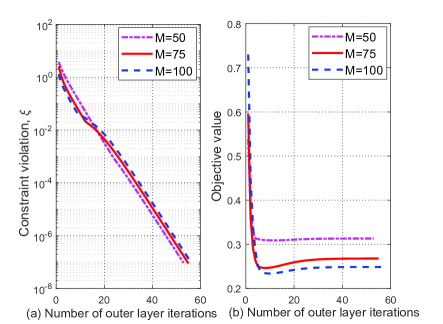
Figure 2: Convergence behaviour of Algorithm 1.

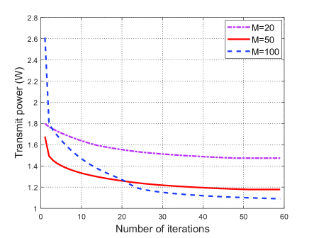
Figure 3: Convergence behaviour of Algorithm 2.

V-A Convergence Behavior of the Proposed Two Algorithms

Before discussing the system performance, we first verify the effectiveness of the proposed penalty-based and SDR-based algorithms, i.e., Algorithm 1 and Algorithm 2, respectively.

Fig. 3 shows the constraint violation and convergence of Algorithm 1 by solving problem (7) with $K=5$ for different number of IRS reflecting elements, namely, $M=50$, $M=75$, and $M=100$. From Fig. 3(a), it is observed that constraint violation $\xi$ decreases fast and reaches the predefined accuracy $10^{-7}$ after about $55$ iterations for $M=50$, which indicates that ${\left|{{\bf{h}}_{k}^{H}{{\bf{w}}_{c,i}}-x_{k,i}^{c}}\right|^{2}}$ and $\left\|{{\bf{A}}{{\bf{w}}_{c,i}}-{\bf{y}}_{i}^{c}}\right\|_{\infty}^{2},i\in{\cal K},k\in{\cal K},$ in (35) are forced to approach zero. As such, the equality constraint (8d) in problem (8) is eventually satisfied. Even for large $M$, e.g., $M=100$, the number of outer layer iterations for reaching the predefined accuracy is about $57$ iterations, which again demonstrates the effectiveness of Algorithm 1. In Fig. 3(b), we can observe that the objective value (9a) is not monotonically decreasing with the number of outer layer iterations and fluctuates during the intermediate iterations. This is mainly because when the penalty coefficient $\rho$ is relatively large, the obtained solution does not satisfy the equality in (8d), thus resulting in the oscillatory behavior. However, as $\rho$ becomes very small, the constraint violation is forced to approach the predefined accuracy. Thus, Algorithm 1 is guaranteed to converge finally.

Fig. 3 shows the convergence of Algorithm 2 by solving problem (36) with $K=5$ and $\epsilon_{\rm th}=\infty$ (i.e., ignore cross-correlation constraint (36d)) for different $M$. It is observed that the required transmit power is monotonically decreasing with the number of iterations and converges about $58$ iterations for different setups. This is expected since each subproblem is optimally/locally solved in each iteration, which results in a non-increasing objective value over iterations. In addition, the objective value is lower-bounded by a finite value due to the minimum SINR required by both users and targets. Thus, Algorithm 2 is guaranteed to converge finally.

V-B IRS-aided Radar and Communication

In this subsection, we compare our proposed scheme with several benchmark schemes under different setups. We adopt the following schemes for comparison: (a) No interference: this corresponds to case I and we study four cases, namely, “Commun_only, penalty, no interference”, “Penalty, no interference”, “SDP, no interference”, and “SDP, no IRS, no interference”. For “Commun_only, penalty, no interference”, only communication signals are transmitted by the Radcom BS and the resulting problem is solved by Algorithm 1; For “Penalty, no interference”, both communication signals and radar signals are transmitted; For “SDP, no interference”, both communication signals and radar signals are transmitted and the resulting problem is solved by Algorithm 2; For “SDP, no IRS, no interference”, the IRS is not used. (b) Interference: this corresponds to case II and we study two schemes, namely, “SDP, interference” and “Commun_only, SDP, interference”, and the corresponding problems are solved by Algorithm 2.

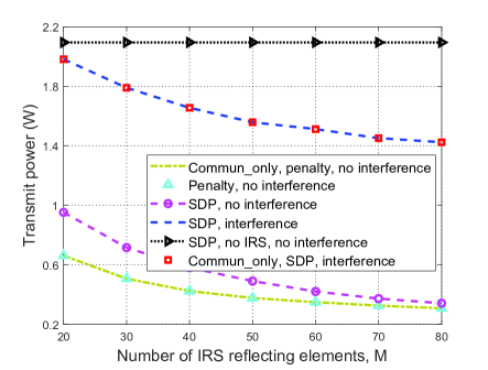
Figure 4: Transmit power versus the number of IRS elements.

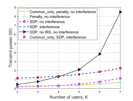
Figure 5: Transmit power versus the number of users.

V-B1 Effect of Number of IRS Reflecting Elements

In Fig. 5, we compare the transmit power obtained by all schemes versus $M$ with $K=5$ and $\epsilon_{\rm th}=\infty$. First, it is observed that with the optimization of IRS phase shifts, the required transmit power monotonically decreases with $M$, even when the interference exists. This is because that installing more reflecting elements at the IRS is able to provide higher passive beamforming gain towards the desired users, thereby reducing transmit power. Second, it is observed that with the IRS, the schemes without interference significantly outperform those with interference as expected. Third, the “Commun_only, penalty, no interference” scheme achieves the same performance with the “Penalty, no interference” scheme, which implies the radar signals are unnecessary and justifies Theorem 1. In addition, we also observe the same results for the case with interference, which justifies Theorem 3. Last, the penalty-based algorithm achieves lower transmit power than the SDP-based algorithm. This is because that with the proper variables partitioning, there is no constraint coupling between the variables in different blocks as shown in Algorithm 1, while it does not hold in Algorithm 2.

V-B2 Effect of Number of Users

In Fig. 5, we compare the transmit power obtained by all schemes versus $K$ with $M=50$ and $\epsilon_{\rm th}=\infty$. It is observed that the required transmit power obtained by all schemes is monotonically increasing as $K$ increases. This is because that the required transmit power highly depends on the user who has the worst channel quality to satisfy the minimum SINR. In addition, we observe that the scheme without IRS requires much higher transmit power than those with IRS in the without interference case, especially when $K$ becomes large, which demonstrates the benefits of applying IRS in the Radcom system. Furthermore, we observe that the scheme with only communication signal transmission achieves the same transmit power with the joint signal transmission, which again justifies Theorem 1 and Theorem 3.

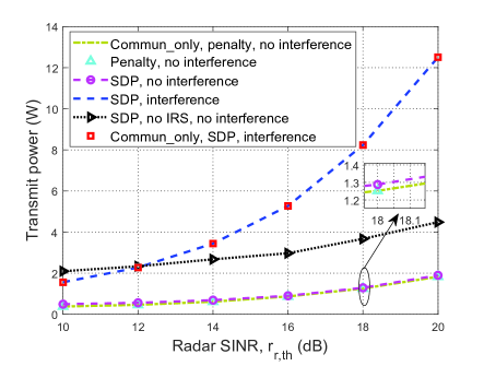
Figure 6: Transmit power versus the Radar SINR.

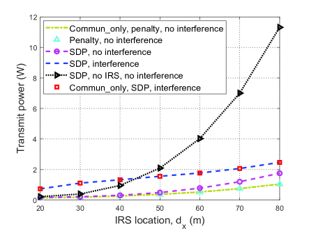
Figure 7: Transmit power versus the Radar SINR.

V-B3 Effect of Radar SINR

In Fig. 7, we study the impact of radar SINR $r_{r,\rm th}$ on the transmit power required at the Radcom BS with $K=5$, $M=50$, $\epsilon_{\rm th}=\infty$, and $r_{c,\rm th}=20~{}{\rm dB}$. We observe that the required transmit power obtained by the scheme with interference remarkably increases as compared with that obtained by the scheme without interference, especially when the required $r_{r,\rm th}$ is high. This is because that as $r_{r,\rm th}$ becomes large, the interference introduced by the IRS will be more prominent, which thus requires higher transmit power to satisfy the radar SINR. However, if the interference can be perfectly canceled, the scheme with the IRS achieves much lower transmit power than that without IRS due to the high passive beamforming gains brought by the IRS.

V-B4 Effect of IRS deployment

In Fig. 7, we study the impact of IRS deployment/location $d_{x}$ on the system performance with $M=50$, $K=5$, and $\epsilon_{\rm th}=\infty$. We observe that as $d_{x}$ increases, i.e., the distance between the IRS and the Radcom BS becomes larger, the required transmit power is remarkably increased by the scheme without IRS due to the high path-loss attenuation. In addition, the performance gap between “SDP, no interference” and “SDP, no IRS, no interference” becomes more pronounced when the IRS is far away from the Radcom BS, which further demonstrates the benefits brought by the IRS. However, this result does not hold for the schemes with interference. To be specific, when $d_{x}\leq 45$, the “SDP, interference” scheme consumes more transmit power than the ‘SDP, no IRS, no interference” scheme, while when $d_{x}\geq 45$, the “SDP, interference” scheme saves more transmit power than the ‘SDP, no IRS, no interference” scheme. This is because as the IRS is deployed close to the Radcom, i.e., $d_{x}\leq 45$, the interference introduced by the IRS is significant, thus impairing the system performance. However, as the IRS is far away from the Radcom, i.e., $d_{x}\geq 45$, the interference introduced by the IRS becomes small. To see it clearly, it is observed that the performance gap between “SDP, interference” and “SDP, no interference” becomes smaller as $d_{x}$ increases, which indicates that the impact of interference introduced by the IRS on the Radcom becomes smaller.

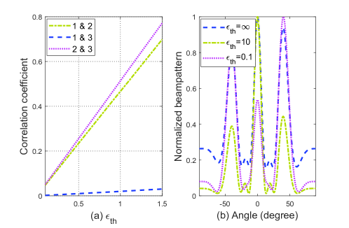
Figure 8: Beampattern design.

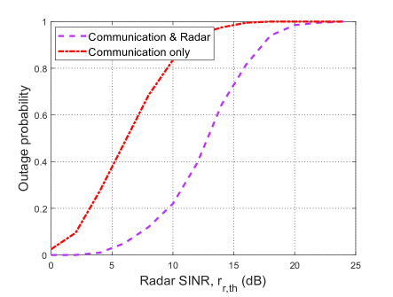
Figure 9: Outage probability versus Radar SINR.

V-B5 Effect of Cross-Correlation Constraint

In Fig. 9(a), we study the impact of $\epsilon_{\rm th}$ on the cross-correlation coefficients of the three target reflected signals. It is observed that when $\epsilon_{\rm th}$ approaches zero, i.e., $\xi_{\rm th}=0.1$, which implies that a stringent cross-correlation is imposed, and all cross-correlation coefficients are very small. However, as $\epsilon_{\rm th}$ becomes large, the first and second reflected signals, i.e., $1~{}\&~{}2$, and the second and third reflected signals, i.e., $2~{}\&~{}3$, are highly correlated, which can degrade significantly the performance of any adaptive technique for the multi-target radar detection [48]. An example of the normalized magnitudes of beampatterns obtained for different $\epsilon_{\rm th}$ under ${\beta_{l}}={\sigma_{\beta}},l\in{\cal L}$ is studied in Fig.  9(b). We can observe that all the schemes with different $\epsilon_{\rm th}$ can track targets well, and the beampatterns obtained with $\epsilon_{\rm th}=\infty$ is better than that with the other cross-correlation constraint, i.e., $\epsilon_{\rm th}=0.1$ and $\epsilon_{\rm th}=10$.

V-B6 Single Waveform versus Joint Waveforms

To evaluate the impact of the single weaveform design and the joint waveform design on the system performance. In Fig. 9, we study the outage probability versus Radar SINR $r_{r,\rm th}$ in case II for different transmit beamforming schemes with $K=5$, $M=50$, $d_{x}=20$, and $\epsilon_{\rm th}=1$. Two schemes are compared: 1) Communication & Radar: both the communication and radar signals are used for transmission and the resulting problem is solved by Algorithm 2; 2) Communication only: only the communication signal is used for transmission and the resulting problem is solved by Algorithm 2 but the Gaussian randomization technique is applied for reconstructing rank-one solution (Here, $1000$ Gaussian randomization realizations are performed). It is observed that the outage probability obtained by the two schemes increases as $r_{r,\rm th}$ increases and finally approaches $1$ for large $r_{r,\rm th}$. This is expected since the higher transmit power is required for satisfying the stringent Radar SINR constraint, thereby potentially increasing the cross-correlation coefficient in (36d) and making the problem infeasible with a higher probability. In addition, it is observed that the “Communication & Radar” scheme performs better than the “Communication only” scheme, which indicates that the radar signal is useful for system design.

VI Conclusion

In this paper, we studied the joint design of active beamforming and passive beamforming for an IRS-aided Radcom system. The transmit power minimization problems for two cases, i.e., case I and case II, based on the presence or absence of the radar cross-correlation design and the interference introduced by the IRS on the Radcom BS were formulated. We first studied case I and proved that the dedicated radar signals are not required, and then proposed a penalty-based algorithm to solve the formulated non-convex optimization problem. Then, we studied case II and showed that the dedicated radar signals are required in general to enhance the system performance, and an SDR-based AO algorithm is proposed to solve this challenging optimization problem. Simulation results demonstrated the benefits of the IRS used for enhancing the performance of the Radcom system. In addition, the results also showed for case II that adopting dedicated radar signals at the Radcom BS can significantly reduce the system outage probability as compared to the case without adopting the dedicated radar signals.

Appendix A: Proof of theorem 1

We prove Theorem 1 by solving the SDR of problem (7). Specifically, define ${{\mathbf{Z}}_{r}}={{\mathbf{W}}_{r}}{\mathbf{W}}_{r}^{H}$ and ${{\bf{W}}_{c,k}}={{\bf{w}}_{c,k}}{\bf{w}}_{c,k}^{H},k\in{\cal K}$, which need to satisfy ${\bf Z}_{r}\succeq{\bf 0},$${{\bf{W}}_{c,k}}\succeq{\bf{0}}$, and ${\rm{rank}}\left({{{\bf{W}}_{c,k}}}\right)=1$. By ignoring the above rank-one constraint on ${{\mathbf{W}}_{c,k}}$’s, the SDR of problem (7) for any given IRS phase shifts $\bf v$ is given by

$$\mathop{\min}\limits_{\left\{{{{\mathbf{W}}_{c,k}}}\right\},{{\mathbf{Z}}_{r}}}\sum\limits_{k=1}^{K}{{\text{tr}}}\left({{{\mathbf{W}}_{c,k}}}\right)+{\text{tr}}\left({{{\mathbf{Z}}_{r}}}\right)$$ (49a)

$${\rm s.t.}~{}{\mathbf{h}}_{k}^{H}\left({\sum\limits_{k=1}^{K}{{{\mathbf{W}}_{c,k}}}+{{\mathbf{Z}}_{r}}}\right){{\mathbf{h}}_{k}}+{\sigma^{2}}\leq\left({\frac{1}{{{r_{k,{\text{th}}}}}}+1}\right){\mathbf{h}}_{k}^{H}{{\mathbf{W}}_{c,k}}{{\mathbf{h}}_{k}},k\in{\cal K},$$ (49b)

$$\qquad{\text{tr}}\left({{\mathbf{A}}\left({\sum\limits_{k=1}^{K}{{{\mathbf{W}}_{c,k}}}+{{\mathbf{Z}}_{r}}}\right){{\mathbf{A}}^{H}}}\right)\geq{r_{r,{\rm{th}}}}{{\sigma}^{2}}.$$ (49c)

It is not difficult to see that problem (49) is a semidefinite programming (SDP) problem and satisfies the Slater’s condition, which indicates that the duality gap is zero. Thus, we consider the following Lagrangian of problem (49) given by

$${{\cal L}_{1}}\left\{{\left\{{{{\mathbf{W}}_{c,k}}}\right\},{{\mathbf{Z}}_{r}},\left\{{{\lambda_{1,k}}}\right\},\mu}\right\}=\sum\limits_{k=1}^{K}{{\text{tr}}}\left({{{\mathbf{B}}_{k}}{{\mathbf{W}}_{c,k}}}\right)+{\text{tr}}\left({{\mathbf{C}}{{\mathbf{Z}}_{r}}}\right)+\sum\limits_{k=1}^{K}{{\lambda_{1,k}}{\sigma^{2}}}+\mu\sigma^{2}{r_{r,{\text{th}}}},$$ (50)

where

$${{\mathbf{B}}_{k}}={{\mathbf{I}}_{{N_{t}}}}+\sum\limits_{i\neq k}^{K}{{\lambda_{1,i}}{{\mathbf{h}}_{i}}{\mathbf{h}}_{i}^{H}}-{{{\lambda_{1,k}}{{\mathbf{h}}_{k}}{\mathbf{h}}_{k}^{H}}}/{{{r_{k,{\text{th}}}}}}-\mu{{\mathbf{A}}^{H}}{\mathbf{A}},k\in{\cal K},$$ (51)

$${\mathbf{C}}={{\mathbf{I}}_{{N_{t}}}}+\sum\limits_{k=1}^{K}{{\lambda_{1,k}}{{\mathbf{h}}_{k}}{\mathbf{h}}_{k}^{H}}-\mu{{\mathbf{A}}^{H}}{\mathbf{A}},$$ (52)

and ${\left\{{{\lambda_{1,k}}}\geq 0\right\}}$ and $\mu\geq 0$ are the dual variables associated with constraints (49b) and (49c), respectively. Denote by dual function ${f_{1}}\left\{{\left\{{{\lambda_{1,k}}}\right\},\mu}\right\}=\mathop{\min}\limits_{\left\{{{{\mathbf{W}}_{c,k}}}\right\},{{\mathbf{Z}}_{r}}}{{\cal L}_{1}}\left\{{\left\{{{{\mathbf{W}}_{c,k}}}\right\},{{\mathbf{Z}}_{r}},\left\{{{\lambda_{1,k}}}\right\},\mu}\right\}$, we have the following lemma:

Lemma 1: To make dual function ${f_{1}}\left\{{\left\{{{\lambda_{1,k}}}\right\},\mu}\right\}$ bounded, we must have

$${\mathbf{C}}\succeq{\mathbf{0}},~{}~{}{{\mathbf{B}}_{k}}\succeq{\mathbf{0}},k\in{\cal K}.$$ (53)

Proof: This can be proved by contradiction. Suppose that ${{\mathbf{B}}_{k}}$ $({\mathbf{C}})$ has at least one negative eigenvalue, we can always construct a solution of ${{{\mathbf{W}}_{c,k}}}$ $({{{\mathbf{Z}}_{r}}})$ that has the same eigenvectors with ${{\mathbf{B}}_{k}}$ $({\mathbf{C}})$, while the eigenvalues of ${{{\mathbf{W}}_{c,k}}}$ $({{{\mathbf{Z}}_{r}}})$ corresponding to ${{\mathbf{B}}_{k}}$ $({\mathbf{C}})$ with negative eigenvalues are set to be positive infinity, resulting in ${\text{tr}}\left({{{\mathbf{B}}_{k}}{{\mathbf{W}}_{c,k}}}\right)\to-\infty$ and ${\text{tr}}\left({{\mathbf{C}}{{\mathbf{Z}}_{r}}}\right)\to-\infty$. This thus completes the proof.  

Accordingly, the dual problem of (49) is given by

$$\mathop{\max}\limits_{\left\{{{\lambda_{1,k}}\geq 0}\right\},\mu\geq 0}\sum\limits_{k=1}^{K}{{\lambda_{1,k}}{\sigma^{2}}}+\mu\sigma_{r}^{2}{r_{r,{\text{th}}}}$$ (54a)

$${\rm s.t.}~{}{\bf C}\succeq{\mathbf{0}},~{}~{}{{\mathbf{B}}_{k}}\succeq{\mathbf{0}},k\in{\cal K}.$$ (54b)

Based on Lemma $1$, it is not difficult to prove that at optimal solutions $\left\{{{\mathbf{W}}_{c,k}^{{\text{opt}}},{\mathbf{Z}}_{r}^{{\text{opt}}}}\right\}$ to minimize (50) for fixed dual variables, the following equalities must hold:

$${\rm{tr}}\left({{{\bf{C}}^{{\rm{opt}}}}{\bf{Z}}_{r}^{{\rm{opt}}}}\right)=0,\;\;{\rm{tr}}\left({{\bf{B}}_{k}^{{\rm{opt}}}{\bf{W}}_{c,k}^{{\rm{opt}}}}\right)=0,k\in{\cal K},$$ (55)

which are equivalent to ${{{\mathbf{C}}^{{\text{opt}}}}{\mathbf{Z}}_{r}^{{\text{opt}}}}={\bf 0}$ and ${{\mathbf{B}}_{k}^{{\text{opt}}}{\mathbf{W}}_{c,k}^{{\text{opt}}}}={\bf 0},k\in{\cal K}$.

To prove Theorem 1, we need to prove that the optimal solutions of problem (49) should satisfy ${\text{rank}}\left({{\mathbf{W}}_{c,k}^{{\text{opt}}}}\right)=1,k\in{\cal K}$, and ${\mathbf{Z}}_{r}^{{\text{opt}}}={\mathbf{0}}$. To proceed it, we consider the following two cases: 1) $\lambda_{1,k}^{{\text{opt}}}=0$ for $k\in{\cal K}$; 2) at least one $\lambda_{1,k}^{{\text{opt}}}$ for $k\in{\cal K}$ is not equal to zero.

For the first case, it is not difficult to see that ${{\mathbf{C}}^{{\text{opt}}}}{\text{ = }}{\mathbf{B}}_{k}^{{\text{opt}}}{\text{ = }}{{\mathbf{I}}_{{N_{t}}}}-{\mu^{{\text{opt}}}}{{\mathbf{A}}^{H}}{\mathbf{A}},k\in{\cal K}$. To guarantee ${{\mathbf{B}}_{k}^{\rm opt}}\succeq{\mathbf{0}},k\in{\cal K}$, and maximize dual problem (54), the optimal dual variable ${\mu^{{\text{opt}}}}$ should satisfy ${\mu^{{\text{opt}}}}=1/{\pi_{\max}}$, where ${\pi_{\max}}$ represents the maximum eigenvalue of ${{\mathbf{A}}^{H}}{\mathbf{A}}$. Under the assumption that amplitudes of targets are independently distributed, i.e., the non-zero singular values of ${\bf A}^{H}{\bf A}$ are not the same, ${{{\mathbf{C}}^{{\text{opt}}}}}$ and ${{\mathbf{B}}_{k}^{{\text{opt}}}}$ must have only one zero eigenvalue and satisfy ${\text{rank}}\left({{{\mathbf{C}}^{{\text{opt}}}}}\right)={\text{rank}}\left({{\mathbf{B}}_{k}^{{\text{opt}}}}\right)={N_{t}}-1,k\in{\cal K}$. Denote by ${{\bf v}_{\max}}$ the eigenvector corresponding to the maximum eigenvalue of ${{\mathbf{A}}^{H}}{\mathbf{A}}$. It is readily to see that ${\mathbf{Z}}_{r}^{{\text{opt}}}$ and ${\mathbf{W}}_{c,k}^{{\text{opt}}}$ should all lie in the subspace spanned by ${{\bf v}_{\max}}$. This indicates that all communication beams should point towards the targets rather than the communication users and the minimum user SINR requirements in (49b) will not be satisfied any more. Obviously, the case of $\lambda_{1,k}^{{\text{opt}}}=0,k\in{\cal K}$, cannot occur here.

For the second case, with any given ${\mathbf{Z}}_{r}^{{\text{opt}}}\succeq{\bf 0}$ satisfying (55), we have

$$-\left({{1}/{{{r_{k,{\text{th}}}}}}+1}\right){\lambda_{1,k}^{\rm opt}}{\mathbf{h}}_{k}^{H}{\mathbf{Z}}_{r}^{{\text{opt}}}{{\mathbf{h}}_{k}} ={\text{tr}}\left({{{\mathbf{C}}^{{\text{opt}}}}{\mathbf{Z}}_{r}^{{\text{opt}}}-\left({{1}/{{{r_{k,{\text{th}}}}}}+1}\right){\lambda_{1,k}}{{\mathbf{h}}_{k}}{\mathbf{h}}_{k}^{H}{\mathbf{Z}}_{r}^{{\text{opt}}}}\right)$$

$$={\text{tr}}\left({{\mathbf{B}}_{k}^{{\text{opt}}}{\mathbf{Z}}_{r}^{{\text{opt}}}}\right)\geq 0,$$ (56)

where the first equality follows from (55), the second equality follows from (51) and (52), and the last inequality holds since both ${{\mathbf{B}}_{k}^{{\text{opt}}}}$ and ${{\mathbf{Z}}_{r}^{{\text{opt}}}}$ are positive semidefinite matrices. From (56), we can derive $\lambda_{1,k}^{{\text{opt}}}{\text{tr}}\left({{{\mathbf{h}}_{k}}{\mathbf{h}}_{k}^{H}{\mathbf{Z}}_{r}^{{\text{opt}}}}\right)=0$ since $\lambda_{1,k}^{{\text{opt}}}\geq 0$ and ${\mathbf{h}}_{k}^{H}{\mathbf{Z}}_{r}^{{\text{opt}}}{{\mathbf{h}}_{k}}\geq 0$, $k\in{\cal K}$. As a result, based on (55) and together with $\lambda_{1,k}^{{\text{opt}}}{\text{tr}}\left({{{\mathbf{h}}_{k}}{\mathbf{h}}_{k}^{H}{\mathbf{Z}}_{r}^{{\text{opt}}}}\right)=0$, we have

$$\left({{{\mathbf{I}}_{{N_{t}}}}-{\mu^{{\text{opt}}}}{{\mathbf{A}}^{H}}{\mathbf{A}}}\right){\mathbf{Z}}_{r}^{{\text{opt}}}=\left({{{\mathbf{I}}_{{N_{t}}}}+\sum\limits_{k=1}^{K}{{\lambda_{1,k}^{\rm opt}}{{\mathbf{h}}_{k}}{\mathbf{h}}_{k}^{H}}-\mu{{\mathbf{A}}^{H}}{\mathbf{A}}}\right){\mathbf{Z}}_{r}^{{\text{opt}}}={\mathbf{0}}.$$ (57)

Suppose that $\lambda_{1,m}^{{\text{opt}}}$ is the non-zero eigenvalue, i.e., $\lambda_{1,m}^{{\text{opt}}}>0$, it follows that ${{{\mathbf{h}}_{m}}{\mathbf{h}}_{m}^{H}{\mathbf{Z}}_{r}^{{\text{opt}}}}={\bf 0}$. Since the non-zero singular values of ${\bf A}^{H}{\bf A}$ are not the same, we have ${\text{rank}}\left({{{\mathbf{I}}_{{N_{t}}}}-{\mu^{{\text{opt}}}}{{\mathbf{A}}^{H}}{\mathbf{A}}}\right)\geq{N_{t}}-1$. This indicates that two matrices ${{{\mathbf{I}}_{{N_{t}}}}-{\mu^{{\text{opt}}}}{{\mathbf{A}}^{H}}{\mathbf{A}}}$ and ${{{\mathbf{h}}_{m}}{\mathbf{h}}_{m}^{H}}$ span the entire space with probability one under the assumption that amplitudes of targets and user channels are uncorrelated. As such, we must have ${\mathbf{Z}}_{r}^{{\text{opt}}}={\mathbf{0}}$.

Next, we show to prove ${\text{rank}}\left({{\mathbf{W}}_{c,k}^{{\text{opt}}}}\right)=1,k\in{\cal K}$. On the one hand, based on (55), it follows that ${\text{rank}}\left({{\mathbf{B}}_{k}^{{\text{opt}}}}\right)\leq{N_{t}}-1$ since ${{\mathbf{W}}_{c,k}^{\rm opt}}\neq{\mathbf{0}}$ (otherwise the communication user SINR constraint (49b) will not be satisfied). On the other hand, recall that any ${\mathbf{Z}}_{r}^{{\text{opt}}}\succeq{\bf 0}$ satisfying (55) should be $0$, it follows that ${\text{rank}}\left({{{\mathbf{C}}^{{\text{opt}}}}}\right)={N_{t}}$. Based on (51) and (52), we have

$${\text{rank}}\left({{\mathbf{B}}_{k}^{{\text{opt}}}}\right) ={\text{rank}}\left({{{\mathbf{C}}^{{\text{opt}}}}-\left({{1}/{{{r_{k,{\text{th}}}}}}+1}\right)\lambda_{1,k}^{{\text{opt}}}{{\mathbf{h}}_{k}}{\mathbf{h}}_{k}^{H}}\right)$$

$$\geq{\text{rank}}\left({{{\mathbf{C}}^{{\text{opt}}}}}\right)-{\text{rank}}\left({\left({{1}/{{{r_{k,{\text{th}}}}}}+1}\right)\lambda_{1,k}^{{\text{opt}}}{{\mathbf{h}}_{k}}{\mathbf{h}}_{k}^{H}}\right)$$

$$={N_{t}}-1.$$ (58)

Thus, combining arguments ${\mathbf{B}}_{k}^{{\text{opt}}}\leq{N_{t}}-1$ and ${\mathbf{B}}_{k}^{{\text{opt}}}\geq{N_{t}}-1$, we have ${\mathbf{B}}_{k}^{{\text{opt}}}={N_{t}}-1,k\in{\cal K}$. Based on (55), it follows ${\text{rank}}\left({{\mathbf{W}}_{c,k}^{{\text{opt}}}}\right)=1,k\in{\cal K}$. Together with the facts that ${\mathbf{Z}}_{r}^{{\text{opt}}}={\mathbf{0}}$ and ${\text{rank}}\left({{\mathbf{W}}_{c,k}^{{\text{opt}}}}\right)=1,k\in{\cal K}$, we can conclude that problem (49) is equivalent to problem (7) and no radar beams are required, which completes the proof.

Appendix B: Proof of lemma 2

To show Lemma $2$, we expand Lagrangian function (19) as

$${{\cal L}_{2}}\left({x_{k,i}^{c},{\lambda_{2,k}}}\right) =\left({1-{\lambda_{2,k}}}\right){\left|{x_{k,k}^{c}}\right|^{2}}-2{\text{Re}}\left\{{x_{k,k}^{c,H}{\mathbf{h}}_{k}^{H}{{\mathbf{w}}_{c,k}}}\right\}+{\left|{{\mathbf{h}}_{k}^{H}{{\mathbf{w}}_{c,k}}}\right|^{2}}$$

$$+\sum\limits_{i\neq k}^{K}{\left({{{\left|{{\mathbf{h}}_{k}^{H}{{\mathbf{w}}_{c,i}}-x_{k,i}^{c}}\right|}^{2}}+{\lambda_{2,k}}{r_{k,{\text{th}}}}{{\left|{x_{k,i}^{c}}\right|}^{2}}}\right)}+{\lambda_{2,k}}{r_{k,{\text{th}}}}{\sigma^{2}}.$$ (59)

To make dual function $f_{2}\left({{\lambda_{2,k}}}\right)=\mathop{\min}\limits_{x_{k,i}^{c}}{\cal L}_{2}\left({x_{k,i}^{c},{\lambda_{2,k}}}\right)$ bounded, we should make $1-{\lambda_{2,k}}>0$, i.e., ${\lambda_{2,k}}<1$, since otherwise we can always set $x_{k,k}^{c}=\kappa{\bf{h}}_{k}^{H}{{\bf{w}}_{c,k}}$ and let $\kappa$ to be positive infinity, which will make ${f_{2}}\left({{\lambda_{2,k}}}\right)$ unbounded. This thus completes the proof of Lemma $2$.

Appendix C: Proof of Theorem 2

Suppose that $\left\{{{{{\mathbf{\bar{W}}}}_{c,k}},{{{\mathbf{\bar{Z}}}}_{r}}}\right\}$ are the converged solutions obtained by AO approach to problem (36). We then construct another new solutions $\left\{{{{{\mathbf{\hat{W}}}}_{c,k}},{{{\mathbf{\hat{Z}}}}_{r}}}\right\}$ that satisfy

$${{{\mathbf{\hat{w}}}}_{c,k}}={\left({{\mathbf{h}}_{k}^{H}{{{\mathbf{\bar{W}}}}_{c,k}}{{\mathbf{h}}_{k}}}\right)^{-1/2}}{{{\mathbf{\bar{W}}}}_{c,k}}{{\mathbf{h}}_{k}},~{}~{}{{{\mathbf{\hat{W}}}}_{c,k}}={{{\mathbf{\hat{w}}}}_{c,k}}{\mathbf{\hat{w}}}_{c,k}^{H},k\in{\cal K},$$ (60)

$${{{\mathbf{\hat{Z}}}}_{r}}=\sum\limits_{k=1}^{K}{{{{\mathbf{\bar{W}}}}_{c,k}}}+{{{\mathbf{\bar{Z}}}}_{r}}-\sum\limits_{k=1}^{K}{{{{\mathbf{\hat{W}}}}_{c,k}}},k\in{\cal K}.$$ (61)

To prove Theorem 2, we need to prove: 1) ${\text{rank}}\left({{{{\mathbf{\hat{W}}}}_{c,k}}}\right)=1,{{{\mathbf{\hat{W}}}}_{c,k}}\succeq{\mathbf{0}},{{{\mathbf{\hat{Z}}}}_{r}}\succeq{\mathbf{0}}$; 2) the objective value obtained by $\left\{{{{{\mathbf{\hat{W}}}}_{c,k}},{{{\mathbf{\hat{Z}}}}_{r}}}\right\}$ in (36a) remains unchanged ; 3) all constraints (36b)-(36d) are still satisfied.

First, based on (60), it is not difficult to check that the newly constructed solutions ${{{\mathbf{\hat{W}}}}_{c,k}},k\in{\cal K}$ are rank-one and positive semidefinite, i.e., satisfy ${\text{rank}}\left({{{{\mathbf{\hat{W}}}}_{c,k}}}\right)=1,{{{\mathbf{\hat{W}}}}_{c,k}}\succeq{\mathbf{0}}$. In addition, for any ${\bm{\phi}}\in{{\mathbb{C}}^{{N_{t}}\times 1}}\neq{\mathbf{0}}$, we have

$${{\bm{\phi}}^{H}}\left({{{{\mathbf{\bar{W}}}}_{c,k}}-{{{\mathbf{\hat{W}}}}_{c,k}}}\right){\bm{\phi}} ={{\bm{\phi}}^{H}}{{{\mathbf{\bar{W}}}}_{c,k}}{\bm{\phi}}-{\left({{\mathbf{h}}_{k}^{H}{{{\mathbf{\bar{W}}}}_{c,k}}{{\mathbf{h}}_{k}}}\right)^{-1}}{\left|{{{\bm{\phi}}^{H}}{{{\mathbf{\bar{W}}}}_{c,k}}{{\mathbf{h}}_{k}}}\right|^{2}}\geq 0,$$ (62)

where the last inequality follows from identity ${\left|{{{\bm{\phi}}^{H}}{{{\mathbf{\bar{W}}}}_{c,k}}{{\mathbf{h}}_{k}}}\right|^{2}}\leq\left({{{\bm{\phi}}^{H}}{{{\mathbf{\bar{W}}}}_{c,k}}{\bm{\phi}}}\right)\left({{\mathbf{h}}_{k}^{H}{{{\mathbf{\bar{W}}}}_{c,k}}{{\mathbf{h}}_{k}}}\right)$ according to the Cauchy-Schwarz inequality. From (62), it indicates that ${{{\mathbf{\bar{W}}}}_{c,k}}-{{{\mathbf{\hat{W}}}}_{c,k}}\succeq{\mathbf{0}}$. Thus, we can see from (61) that ${{{{\mathbf{\hat{Z}}}}_{r}}}$ can be rewrote as the summation of $K+1$ positive semidefinite matrices, it follows that ${{{\mathbf{\hat{Z}}}}_{r}}\succeq{\mathbf{0}}$.

Second, the expression $\sum\limits_{k=1}^{K}{{{{\mathbf{\hat{W}}}}_{c,k}}}+{{{\mathbf{\hat{Z}}}}_{r}}$ can be recast as

$$\sum\limits_{k=1}^{K}{{{{\mathbf{\hat{W}}}}_{c,k}}}+{{{\mathbf{\hat{Z}}}}_{r}}=\sum\limits_{k=1}^{K}{{{{\mathbf{\hat{W}}}}_{c,k}}}+\sum\limits_{k=1}^{K}{{{{\mathbf{\bar{W}}}}_{c,k}}}+{{{\mathbf{\bar{Z}}}}_{r}}-\sum\limits_{k=1}^{K}{{{{\mathbf{\hat{W}}}}_{c,k}}}=\sum\limits_{k=1}^{K}{{{{\mathbf{\bar{W}}}}_{c,k}}}+{{{\mathbf{\bar{Z}}}}_{r}},$$ (63)

where the first equality follows from (61). Thus, we have $\sum\limits_{k=1}^{K}{{\text{tr}}}\left({{{{\mathbf{\hat{W}}}}_{c,k}}}\right)+{\text{tr}}\left({{{{\mathbf{\hat{Z}}}}_{r}}}\right)=\sum\limits_{k=1}^{K}{{\text{tr}}}\left({{{{\mathbf{\bar{W}}}}_{c,k}}}\right)+{\text{tr}}\left({{{{\mathbf{\bar{Z}}}}_{r}}}\right)$, which shows that the objective value remains unchanged.

Third, substituting (60) into ${\mathbf{h}}_{k}^{H}{{{\mathbf{\hat{W}}}}_{c,k}}{{\mathbf{h}}_{k}}$, we have

$${\mathbf{h}}_{k}^{H}{{{\mathbf{\hat{W}}}}_{c,k}}{{\mathbf{h}}_{k}}={\mathbf{h}}_{k}^{H}{{{\mathbf{\hat{w}}}}_{c,k}}{\mathbf{\hat{w}}}_{c,k}^{H}{{\mathbf{h}}_{k}}={\mathbf{h}}_{k}^{H}{{{\mathbf{\bar{W}}}}_{c,k}}{\mathbf{h}}_{k},k\in{\cal K}.$$ (64)

Combining (64) with (63), we can readily check that constraints (36b)-(36d) are all satisfied. Based on the above results, we complete the proof of Theorem 2.

Appendix D: Proof of Theorem 4

By setting ${{\bf{Z}}_{r}}={\bf{0}}$ in problem (36) and denoting the newly formulated problem as problem (36)-new, it is not difficult to see that any feasible solutions to problem (36)-new are also feasible to problem (36). Denoted by $\left\{{{{{\bf{\tilde{W}}}}_{c,k}},{{{\bf{\tilde{Z}}}}_{r}}}\right\}$ the feasible solutions to problem (36). We can always construct another solutions to problem (36)-new, denoted by $\left\{{{{{\bf{\mathord{\buildrel{\lower 3.0pt\hbox{$\scriptscriptstyle\frown$}}\over{W}}}}}_{c,k}}}\right\}$, satisfying

$${{{\bf{\mathord{\buildrel{\lower 3.0pt\hbox{$\scriptscriptstyle\frown$}}\over{W}}}}}_{c,k}}={{{\bf{\tilde{W}}}}_{c,k}}+{\alpha_{k}}{{{\bf{\tilde{Z}}}}_{r}},~{}\sum\limits_{k=1}^{K}{{\alpha_{k}}}=1,{\alpha_{k}}\geq 0,\forall k,$$ (65)

so that $\sum\limits_{k=1}^{K}{{{{\bf{\mathord{\buildrel{\lower 3.0pt\hbox{$\scriptscriptstyle\frown$}}\over{W}}}}}_{c,k}}}=\sum\limits_{k=1}^{K}{{{{\bf{\tilde{W}}}}_{c,k}}}+{{{\bf{\tilde{Z}}}}_{r}}$ and ${\alpha_{k}}{\bf{h}}_{k}^{H}{{{\bf{\tilde{Z}}}}_{r}}{{\bf{h}}_{k}}\geq 0$, which indicates that any feasible solutions to problem (36) are also feasible to problem (36)-new while with the same objective value. Thus, problem (36) is equivalent to problem (36)-new. This thus completes the proof.

References

• [1] T. S. Rappaport et al., “Millimeter wave mobile communications for 5G cellular: It will work!” IEEE Access, vol. 1, pp. 335–349, May 2013.
• [2] M. Parker, Digital Signal Processing 101: Everything you need to know to get started.   Newnes, 2017.
• [3] L. Zheng, M. Lops, Y. C. Eldar, and X. Wang, “Radar and communication coexistence: An overview: A review of recent methods,” IEEE Signal Process. Mag., vol. 36, no. 5, pp. 85–99, Sept. 2019.
• [4] R. Saruthirathanaworakun, J. M. Peha, and L. M. Correia, “Opportunistic sharing between rotating radar and cellular,” IEEE J. Sel. Areas Commun., vol. 30, no. 10, pp. 1900–1910, Nov. 2012.
• [5] F. Liu, C. Masouros, A. Li, H. Sun, and L. Hanzo, “MU-MIMO communications with MIMO radar: From co-existence to joint transmission,” IEEE Trans. Wireless Commun., vol. 17, no. 4, pp. 2755–2770, Apr. 2018.
• [6] S. Sodagari, A. Khawar, T. C. Clancy, and R. McGwier, “A projection based approach for radar and telecommunication systems coexistence,” in 2012 IEEE GLOBECOM, Anaheim, California, USA, pp. 5010–5014.
• [7] B. Li, A. P. Petropulu, and W. Trappe, “Optimum co-design for spectrum sharing between matrix completion based MIMO radars and a MIMO communication system,” IEEE Trans. Signal Process., vol. 64, no. 17, pp. 4562–4575, Sept. 2016.
• [8] B. Li and A. Petropulu, “MIMO radar and communication spectrum sharing with clutter mitigation,” in 2016 RadarConf, Philadelphia, PA, USA, pp. 1–6.
• [9] A. Hassanien, M. G. Amin, Y. D. Zhang, and F. Ahmad, “Signaling strategies for dual-function radar communications: an overview,” IEEE Aerosp. Electron. Syst. Mag., vol. 31, no. 10, pp. 36–45, Oct. 2016.
• [10] C. Sturm and W. Wiesbeck, “Waveform design and signal processing aspects for fusion of wireless communications and radar sensing,” Proc. IEEE, vol. 99, no. 7, pp. 1236–1259, Jul. 2011.
• [11] A. Hassanien, M. G. Amin, Y. D. Zhang, and F. Ahmad, “Dual-function radar-communications: Information embedding using sidelobe control and waveform diversity,” IEEE Tran. Signal Process., vol. 64, no. 8, pp. 2168–2181, Apr. 2016.
• [12] ——, “Phase-modulation based dual-function radar-communications,” IET Radar, Sonar & Navigation, vol. 10, no. 8, pp. 1411–1421, Apr. 2016.
• [13] A. Şahin, S. S. M. Hoque, and C.-Y. Chen, “Index modulation with circularly-shifted chirps for dual-function radar and communications,” IEEE Trans. Wireless Commun., 2021, early access, doi: 10.1109/TWC.2021.3117063.
• [14] F. Liu, L. Zhou, C. Masouros, A. Li, W. Luo, and A. Petropulu, “Toward dual-functional radar-communication systems: Optimal waveform design,” IEEE Trans. Signal Process., vol. 66, no. 16, pp. 4264–4279, Aug. 2018.
• [15] R. Liu, M. Li, Q. Liu, and A. L. Swindlehurst, “Dual-functional radar-communication waveform design: A symbol-level precoding approach,” IEEE J. Sel. Top. Sign. Proces., vol. 15, no. 6, pp. 1316–1331, Nov. 2021.
• [16] X. Liu, T. Huang, N. Shlezinger, Y. Liu, J. Zhou, and Y. C. Eldar, “Joint transmit beamforming for multiuser MIMO communications and MIMO radar,” IEEE Trans. Signal Process., vol. 68, pp. 3929–3944, Jun. 2020.
• [17] H. Hua, J. Xu, and T. X. Han, “Optimal transmit beamforming for integrated sensing and communication,” 2021. [Online]. Available: https://arxiv.org/abs/2104.11871.
• [18] Q. Wu and R. Zhang, “Towards smart and reconfigurable environment: Intelligent reflecting surface aided wireless network,” IEEE Commun. Mag., vol. 58, no. 1, pp. 106–112, Jan. 2020.
• [19] Q. Wu, S. Zhang, B. Zheng, C. You, and R. Zhang, “Intelligent reflecting surface aided wireless communications: A tutorial,” IEEE Trans. Commun., vol. 69, no. 5, pp. 3313–3351, May 2021.
• [20] Y. Liu, X. Liu, X. Mu, T. Hou, J. Xu, M. Di Renzo, and N. Al-Dhahir, “Reconfigurable intelligent surfaces: Principles and opportunities,” IEEE Commun.Surveys Tuts., vol. 23, no. 3, pp. 1546–1577, 3rd quart. 2021.
• [21] Q. Wu and R. Zhang, “Intelligent reflecting surface enhanced wireless network via joint active and passive beamforming,” IEEE Trans. Wireless Commun., vol. 18, no. 11, pp. 5394–5409, Nov. 2019.
• [22] C. Pan, H. Ren, K. Wang, W. Xu, M. Elkashlan, A. Nallanathan, and L. Hanzo, “Multicell MIMO communications relying on intelligent reflecting surfaces,” IEEE Trans. Wireless Commun., vol. 19, no. 8, pp. 5218–5233, Aug. 2020.
• [23] M. Hua, Q. Wu, D. W. K. Ng, J. Zhao, and L. Yang, “Intelligent reflecting surface-aided joint processing coordinated multipoint transmission,” IEEE Trans. Commun., vol. 69, no. 3, pp. 1650–1665, Mar. 2021.
• [24] G. Zhou, C. Pan, H. Ren, K. Wang, and A. Nallanathan, “Intelligent reflecting surface aided multigroup multicast miso communication systems,” IEEE Trans. Signal Process., vol. 68, pp. 3236–3251, Apr. 2020.
• [25] Q. Wu, X. Zhou, and R. Schober, “IRS-assisted wireless powered NOMA: Do we really need different phase shifts in DL and UL?” IEEE Wireless Commun. Lett., vol. 10, no. 7, pp. 1493–1497, Jul. 2021.
• [26] M. Hua and Q. Wu, “Joint dynamic passive beamforming and resource allocation for IRS-aided full-duplex WPCN,” IEEE Trans. Wireless Commun., 2021, early access, doi: 10.1109/TWC.2021.3133491.
• [27] G. Chen, Q. Wu, W. Chen, D. W. K. Ng, and L. Hanzo, “IRS-aided wireless powered MEC systems: TDMA or NOMA for computation offloading?” 2021. [Online]. Available: https://arxiv.org/abs/2108.06120.
• [28] H. Long et al., “Reflections in the sky: Joint trajectory and passive beamforming design for secure UAV networks with reconfigurable intelligent surface,” 2020. [Online]. Available: https://arxiv.org/abs/2005.10559.
• [29] M. Hua, L. Yang, Q. Wu, C. Pan, C. Li, and A. Lee Swindlehurst, “UAV-assisted intelligent reflecting surface symbiotic radio system,” IEEE Trans. Wireless Commun., vol. 20, no. 9, pp. 5769–5785, Sept. 2021.
• [30] S. Li, B. Duo, M. Di Renzo, M. Tao, and X. Yuan, “Robust secure UAV communications with the aid of reconfigurable intelligent surfaces,” IEEE Trans. Wireless Commun., vol. 20, no. 10, pp. 6402–6417, Oct. 2021.
• [31] X. Mu, Y. Liu, L. Guo, J. Lin, and N. Al-Dhahir, “Exploiting intelligent reflecting surfaces in NOMA networks: Joint beamforming optimization,” IEEE Trans. Wireless Commun., vol. 19, no. 10, pp. 6884–6898, Oct. 2020.
• [32] ——, “Capacity and optimal resource allocation for IRS-assisted multi-user communication systems,” IEEE Trans. Commun., vol. 69, no. 6, pp. 3771–3786, Jun. 2021.
• [33] M. Fu, Y. Zhou, Y. Shi, and K. B. Letaief, “Reconfigurable intelligent surface empowered downlink non-orthogonal multiple access,” IEEE Trans. Commun., vol. 69, no. 6, pp. 3802–3817, Jun. 2021.
• [34] S. Buzzi, E. Grossi, M. Lops, and L. Venturino, “Foundations of MIMO radar detection aided by reconfigurable intelligent surfaces,” 2021. [Online]. Available: https://arxiv.org/abs/2105.09250.
• [35] W. Lu et al., “Target detection in intelligent reflecting surface aided distributed MIMO radar systems,” IEEE Sensors Lett., vol. 5, no. 3, pp. 1–4, Mar. 2021.
• [36] C. J. Vaca-Rubio et al., “Radio sensing with large intelligent surface for 6G,” 2021. [Online]. Available: https://arxiv.org/abs/2111.02783.
• [37] S. Buzzi, E. Grossi, M. Lops, and L. Venturino, “Radar target detection aided by reconfigurable intelligent surfaces,” IEEE Signal Processing Lett., vol. 28, pp. 1315–1319, Jun. 2021.
• [38] Z.-M. Jiang, M. Rihan, P. Zhang, L. Huang, Q. Deng, J. Zhang, and E. M. Mohamed, “Intelligent reflecting surface aided dual-function radar and communication system,” IEEE Systems J., 2021, early access, doi: 10.1109/JSYST.2021.3057400.
• [39] X. Song, D. Zhao, H. Hua, T. X. Han, X. Yang, and J. Xu, “Joint transmit and reflective beamforming for IRS-assisted integrated sensing and communication,” 2021. [Online]. Available: https://arxiv.org/abs/2111.13511.
• [40] X. Wang, Z. Fei, Z. Zheng, and J. Guo, “Joint waveform design and passive beamforming for RIS-assisted dual-functional radar-communication system,” IEEE Trans. Veh. Technol.,, vol. 70, no. 5, pp. 5131–5136, May 2021.
• [41] R. Liu, M. Li, Y. Liu, Q. Wu, and Q. Liu, “Joint transmit waveform and passive beamforming design for RIS-aided DFRC systems,” 2021. [Online]. Available: https://arxiv.org/abs/2112.08861.
• [42] E. Fishler, A. Haimovich, R. Blum, L. Cimini, D. Chizhik, and R. Valenzuela, “Spatial diversity in radars—models and detection performance,” IEEE Trans. Signal Process., vol. 54, no. 3, pp. 823–838, Mar. 2006.
• [43] G. Cui, H. Li, and M. Rangaswamy, “MIMO radar waveform design with constant modulus and similarity constraints,” IEEE Trans. Signal Process., vol. 62, no. 2, pp. 343–353, Jan. 2014.
• [44] Z. Cheng, Z. He, B. Liao, and M. Fang, “MIMO radar waveform design with PAPR and similarity constraints,” IEEE Trans. Signal Process., vol. 66, no. 4, pp. 968–981, Feb. 2018.
• [45] L. Zheng, M. Lops, X. Wang, and E. Grossi, “Joint design of overlaid communication systems and pulsed radars,” IEEE Trans. Signal Process., vol. 66, no. 1, pp. 139–154, Jan. 2018.
• [46] P. Stoica, J. Li, and Y. Xie, “On probing signal design for MIMO radar,” IEEE Trans. Signal Process., vol. 55, no. 8, pp. 4151–4161, Aug. 2007.
• [47] L. Xu, J. Li, and P. Stoica, “Target detection and parameter estimation for MIMO radar systems,” IEEE Trans. Aerosp. Electron. Syst., vol. 44, no. 3, pp. 927–939, Jul. 2008.
• [48] ——, “Radar imaging via adaptive MIMO techniques,” in 2006 14th EUSIPCO, Florence, Italy, pp. 1–5.
• [49] S. Boyd and L. Vandenberghe, Convex Optimization.   Cambridge University Press, 2004.
• [50] Q. Shi, M. Hong, X. Gao, E. Song, Y. Cai, and W. Xu, “Joint source-relay design for full-duplex MIMO AF relay systems,” IEEE Trans. Signal Process., vol. 64, no. 23, pp. 6118–6131, Dec. 2016.
• [51] X.-D. Zhang, Matrix analysis and applications.   Cambridge University Press, 2017.
• [52] N. D. Sidiropoulos, T. N. Davidson, and Z.-Q. Luo, “Transmit beamforming for physical-layer multicasting,” IEEE Trans. Signal Process., vol. 54, no. 6, pp. 2239–2251, Jun. 2006.