Uni6D: A Unified CNN Framework without Projection Breakdown for 6D Pose Estimation

Abstract

As RGB-D sensors become more affordable, using RGB-D images to obtain high-accuracy 6D pose estimation results becomes a better option. State-of-the-art approaches typically use different backbones to extract features for RGB and depth images. They use a 2D CNN for RGB images and a per-pixel point cloud network for depth data, as well as a fusion network for feature fusion. We find that the essential reason for using two independent backbones is the “projection breakdown” problem. In the depth image plane, the projected 3D structure of the physical world is preserved by the 1D depth value and its built-in 2D pixel coordinate (UV). Any spatial transformation that modifies UV, such as resize, flip, crop, or pooling operations in the CNN pipeline, breaks the binding between the pixel value and UV coordinate. As a consequence, the 3D structure is no longer preserved by a modified depth image or feature. To address this issue, we propose a simple yet effective method denoted as Uni6D that explicitly takes the extra UV data along with RGB-D images as input. Our method has a Unified CNN framework for 6D pose estimation with a single CNN backbone. In particular, the architecture of our method is based on Mask R-CNN with two extra heads, one named RT head for directly predicting 6D pose and the other named abc head for guiding the network to map the visible points to their coordinates in the 3D model as an auxiliary module. This end-to-end approach balances simplicity and accuracy, achieving comparable accuracy with state of the arts and 7.2$\times$ faster inference speed on the YCB-Video dataset.

1 Introduction

6D pose estimation plays a fundamental role in emerging applications, e.g., autonomous driving [1, 2, 3], intelligent robotic grasping [4, 5, 6] and augmented reality [7].

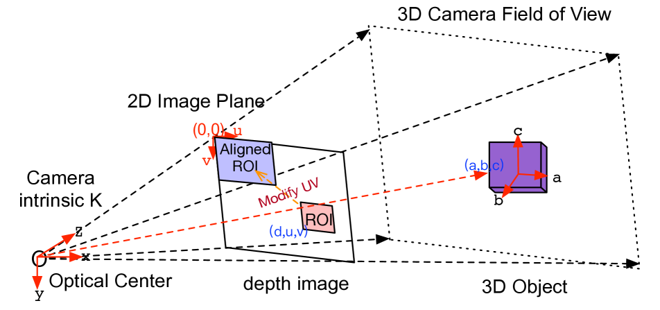
(a) Projection breakdown caused by the RoI transformation, including crop, resize and RoI-Align [8]: The red dotted line connects a 3D object and its projected RoI in the depth image. Any pixel $(d,u,v)$ in the RoI and its corresponding point $(a,b,c)$ on the 3D object follow the projection equation. The equation no longer holds if the built-in coordinate (UV) is modified by RoI-Align, as though the RoI was moved to the top left corner of the image.

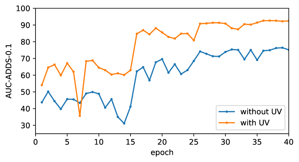
(b) Introducing UV data fixes the problem of projection breakdown and improve the 6D pose estimation performance with various spatial transformations. $x$ axis is the training epoch, and $y$ axis is the testing accuracy.

Figure 1: Visualization and experiment results of projection breakdown problem.

RGB-D sensors provide a direct signal of the surface texture and geometry of the physical 3D world, and as their prices fall, RGB-D images are becoming a more attractive data source for 6D pose estimation.

However, state of the arts [9, 10, 11, 12, 2, 13] typically use two separate backbone networks to extract features for RGB and depth images, with a 2D CNN for RGB images and per-pixel PointNet [14] or PointNet++ [15] for depth data. After these features have been obtained, an additional fusion process is designed to blend them. Existing methods use different backbones to account for the heterogeneity of these two types of data. However, the key reason they can’t extract features with a single backbone is hidden in the classic 3D vision projection equation:

$$\begin{bmatrix}u\\ v\\ 1\end{bmatrix}=\frac{K}{d}\begin{bmatrix}x\\ y\\ d\end{bmatrix}=\frac{K}{R_{z}(a,b,c)+T_{z}}\begin{pmatrix}R\times\begin{bmatrix}a\\ b\\ c\end{bmatrix}+T\end{pmatrix},$$ (1)

which describes a point $(a,b,c)$ first rotated by the rotation matrix $R\in SO(3)$ and translated by $T\in R^{3}$ to the position $(x,y,d)$ in camera coordinate system. It is then projected to the pixel at $(u,v)$ in image plane using the intrinsic matrix $K$ of the camera. The 3D structure of the visible points in the 3D model seen from the camera’s perspective is preserved by the depth value ($d$) of each pixel and its coordinate $(u,v)$ in the depth image. It implies in a single-channel depth image, each pixel value is linked to its built-in coordinates. The plain UV can be used to preserve the 3D structure and changing it will break the 3D projection equation. However, in the traditional CNN pipeline, spatial transformations such as pooling, crop, RoI-Align [8] in the convolution operator, and resize, crop, and flip in data augmentation do change the UV. As shown in Fig. 1(a), when those spatial transformations are applied to a depth image, the projection equation is broken, and we call this “projection breakdown”. This is the primary reason why the traditional CNN pipeline struggles to process RGB images and depth data at the same time.

In this paper, we propose a simple yet effective method to save the projection breakdown: explicitly feeding extra UV data along with depth to 2D CNN. D+UV acts as 3D data, making the value $(d,u,v)$ at each pixel self-complete and decoupling $d$ from its built-in coordinate in the image plane. Given the self-complete information at each pixel, the projection equation still holds after spatial transformations. As a result, we can extract features from RGB-D images using the traditional CNN pipeline, including its data augmentation methods. As shown in Fig 1(b), the accuracy of 6D pose estimation is greatly improved with extra UV data. Extensive experiments show that transformations in data augmentation greatly harm the accuracy without using UV data, but improve the accuracy with UV data is used.

Eq. 1 also indicates that the network should map visible points in an RGB-D image to their original coordinates in the 3D model. As far as we know, Existing keypoint-based 6D pose estimation approaches, such as [6] and [16], learn the 3D offset from visible points to selected keypoints and produce state-of-the-art accuracy. However, these methods require the iterative voting and regression mechanism as a post-process operation, which accounts for 92.9% of total frame processing time in FFB6D [16] and 79.2% in PVN3D [6] on the multiple-object dataset [17]. To achieve an accurate, real-time and practical pipeline, we propose Uni6D, an end-to-end 6D pose estimation network based on Mask R-CNN[8] that uses a unified backbone to extract feature from RGB-D images. Mask R-CNN performs the object detection and instance segmentation with parallel multi-head networks. On its basis, we add an extra RT head to predict the rotation matrix $R$ and the translation vector $T$ directly, with another abc head to carry out the mapping of visible points, instead of using the time-consuming post-processing used in previous works. Without any bells and whistles, Uni6D achieves 95.2% in terms of AUC of ADDS-0.1 on YCB-Video dataset and a real-time inference with 25.6 FPS, which is $7.2\times$ faster than the state of the art. To summarize, the main contributions of this paper are as follows: (1) We expose the “projection breakdown” problem that exists beneath CNN-based depth image processing and introduce the extra UV data into input to fix it, which indicates that a single CNN backbone is all you need for RGB-D feature extraction. (2) We propose an efficient and effective method denoted as Uni6D. The proposed abc head and RT head are optimized in a multitask manner, and we use RT head to directly obtain the pose estimation results. (3) We provide extensive experimental and ablation studies to highlight the benefits of our method, and the results show that our method outperforms existing methods in terms of the time efficiency and achieve promising performance.

2 Related Work

2.1 6DoF Pose Estimation from RGB Images

Holistic methods, keypoint-based approaches and dense correspondence methods are the three types of RGB-only pose estimation methods. Holistic methods [18, 19, 20, 21, 22, 23, 24, 25, 26] directly estimate the 6D pose of objects in an RGB image. They use rigid templates to compute the best match pose or directly regress the 6D pose with deep neural networks. However, non-linearity of the rotation space limits generalization ability of DNN based methods. On the contrary, keypoint-based approaches [27, 28, 29, 30, 31] detect the keypoints of objects and then estimate the pose by finding the 2D and 3D correlations at these points. Dense correspondence methods [32, 33, 34, 35, 36, 37, 38, 39, 40] utilize the correspondence between image pixels and mesh vertexes to estimation the pose with the Perspective-n-Point (PnP) method to recover poses. Although these dense correspondence method can improve robustness in occlusion situations, the performance is damaged by the unlimited output space. However, the performance of all these methods which only uses RGB images are limited by the loss of geometry information. Therefore, many point clouds based methods have been proposed.

2.2 6DoF Pose Estimation from Point Clouds

As the cost of depth sensors decreases and accuracy increases, several point clouds based methods has been proposed. The mainstream methods usually use 3D ConvNets [41, 42] or point cloud network [43, 43] to extract the feature and estimate the 6D pose. However, the performance of these methods are limited by the essential noise and shortcomings of the point clouds data. They do not perform well with the sparse and weakly textured point cloud, which indicates the necessity of RGB data.

2.3 6DoF Pose Estimation from RGB-D Data

Recently, most of 6D pose estimation state-of-the-art approaches utilize the RGB images and depths or point cloud data to achieve a higher accuracy. Classical methods [44, 45, 46, 33, 34, 47, 48] adopt the correspondence grouping and hypothesis verification for the rule based feature and templates of RGB-D data. With the development of deep learning, most data-driven methods use deep neural networks to extract features instead of hand-coded features. They extract features of RGB images and point clouds with independent feature extractors and then fuse them. Most of them [2, 9, 11, 10, 16] use 2D CNN for RGB images and point cloud network for depth data considering the data heterogeneity between them. Since the appearance and geometry features are extracted separately, they need to add more complex structure to iterative fuse two features into one in order to predict poses [9, 11, 10, 16] and enable the communication between the RGB and depth information [16].

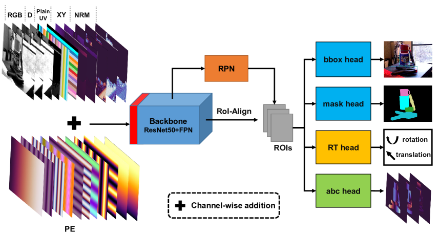
Figure 2: Overview architecture of our Uni6D, which inherits the basic network structure and the simplicity from Mask R-CNN. We add the RGB-D, UV encoding and NRM with PE in a channel-wise manner and feed this new input into the single backbone network. No fusion operation for RGB and depth feature is further required. The red part in the backbone network denotes the channel modification to adapt the RGB-D+UV+NRM (with PE) input, which is to increase the input channel of the first convolutional layer. RT head is used to predict rotation and translation directly and abc head aims to map visible points to their 3D coordinate in its 3D model. With above components, our Uni6D predicts object categories, localization and its RT matrix directly without any post-processing.

2.4 Analysis on State-of-the-art Approaches

As far as we know, the best result is obtained by two keypoint-based approaches, PVN3D [6] and FFB6D [16] for now. As the name implies, keypoint-based approaches design a network to predict the 3D offset from a visible point to some selected keypoints. Based on this offset, each visible point gives a prediction of keypoints in the camera coordinates system, i.e. $(x,y,z)$. An iterative voting mechanism is designed[6] to find the best prediction of keypoints by choosing the clustering with most votes. The coordinates of the keypoints, i.e. $(a,b,c)$ in 3D model, is known before inference. Given some matched pairs of $(a,b,c)$ and $(x,y,z)$, an iterative least-square regression is adopted to get the final 6D pose. We believe that the success of keypoint-based approaches is relies on two reasons: 1) Dense prediction and intelligent de-noising: each visible point will give prediction to visible points and voting is used to filter out bad predictions. Given depth images contain a lot of noise, voting is a great way of de-noising. 2) The 3D offset loss is useful to guide the network mapping visible points to its 3D model at pixel level.

PointNet++[14, 15] requires finding K-nearest neighbors in 3D space. We believe KNN for each pixel, iterative voting and regression are quite heavy when porting to real applications. We find that the essential reason is the aforementioned projection breakdown caused by the change operation on UV. In our work, we reveal and solve the projection breakdown problem and adopt a unified feature extractor of the RGB-D data. Benefited from a unified CNN backbone to extract feature from RGB-D images, we propose a straightforward 6D pose estimation pipeline which directly outputs the detection and pose estimation in an end-to-end manner instead of using time-consuming post-processes.

3 Methodology of the Uni6D

Our goal is to propose an accurate, real-time and practical 6D pose estimation method. To this end, we develop an end-to-end framework named Uni6D, which extracts the feature of RGB-D images through a unified backbone network and directly outputs the 6D pose with a straightforward pipeline. Our framework inherits the concise design of Mask R-CNN [8] and introduces a novel RT head and an abc head into it to obtain the 6D pose. With these two heads, we perform multitask joint optimization for the object classification, detection, segmentation and pose estimation. The overall proposed architecture is illustrated in Fig. 2. In this section, we discuss how to inherit the legacy of the Mask R-CNN (Section 3.1), how to encode UV to fix the projection breakdown (Section 3.2), the structure of the RT head and abc head (Section 3.3), the loss function (Section 3.4) and the inference process (Section 3.5).

3.1 Legacy of Mask R-CNN

Object detection and instance segmentation are usually the first steps in 6D pose estimation. As a widely used practical algorithm, Mask R-CNN is capable of achieving them with satisfactory results. Therefore, we use the Mask R-CNN as the basic network. As shown in Fig. 2. Uni6D inherits the basic network structure from Mask R-CNN, including the ResNet [49] backbone, the FPN [50] for feature pyramid, the RPN to propose RoIs of potential objects, a mask head for segmentation, and a bbox head for object detection and classification. Using one backbone for two heterogeneous data becomes possible after we solve the projection breakdown problem. As a result, rather than using separate backbone networks for RGB images and depth data as in other methods, we simply use a unified backbone network that can be implemented by making minor changes to Mask R-CNN. Furthermore, feature fusion is no longer required. Meanwhile, it is very natural to add the regression task of the RT matrix and abc points in parallel on the original basis of Mask R-CNN. An RT head is proposed to guide the network to map visible points to its 3D model, and an extra abc head is proposed to predict 6D pose directly.

3.2 Encoding UV Data as Input

To overcome the issue of projection breakdown, we add the UV data into the input RGB-D data and feed them together into the unified backbone. For the RGB-D data, we directly combine the RGB image and corresponding depth data along the channel dimension. There are three ways to encode positional information. 1) Plain UV coordinates UV: we directly concatenate this coordinates data with the RGB-D data along the channel dimension. Plain UV is the same height and width with RGB-D images. It has two channels, one channel stores the coordinate of U and the other V, i.e., the value at pixel $(u,v)$ in U-channel is $u$, and in V-channel is $v$. 2) Inverse projected XY: given camera intrinsic matrix $K$ and depth image, we encode corresponding plain UV coordinates $(u,v)$ of each pixel into inverse projected XY $(x,y)$ based on Equation 1. XY has two channels, too. We also concatenate XY with RGB-D data along the channel dimension. 3) Positional encoding PE [51, 52]: positional encoding is widely used in many other fields such as vision transformers [52]. We encode the position with the trigonometric function and add it into the input data. Overall, the aforementioned three forms of UV encoding information have their own advantages. Plain UV is more direct, XY implies the internal reference information, and PE can be added to other input channels to be more integrated. They work together to complete each other and get the best performance. Since depth normal vector is a widely used for depth image, we also concatenate it to the input and denote it as “NRM”.

3.3 RT head and abc head for Multitask Learning

We propose RT head and abc head to predict RT matrix and the points of 3D model, where $R$ is the rotation matrix in the form of quaternion and $T\in R^{3}$ is the translation matrix. These heads are added to Mask R-CNN as two novel parallel branches and take the features of all proposals extracted through RoI-Align as input. As shown in Fig. 3, the RT head in our method has a similar structure with the bbox head in Mask R-CNN, which contains two shared and two independent fully connected layers to obtain the RT matrix. The abc head is similar with the mask head as an FCN structure, which is developed with four $3\times 3$ and one $1\times 1$ convolutional layers to output the 3D points.

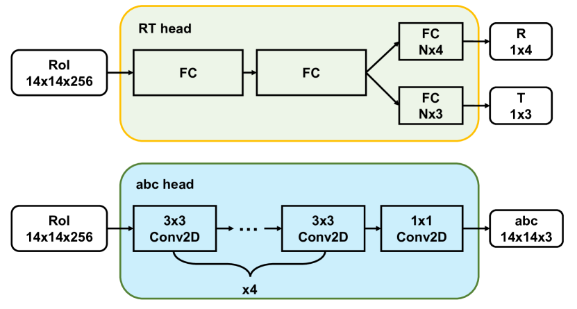
Figure 3: Details of RT head and abc head. Features of all proposals extracted through RoI-Align are used as the input of them. $N$ in the RT head is the number of the input dimension.

3.4 Loss Function

In addition to the classification, detection and segmentation loss functions in the original Mask R-CNN, there are two new loss functions for RT head and abc head. The formula of the RT head loss $\mathcal{L}_{rt}$ is:

$$\begin{split}\mathcal{L}_{rt}=\frac{1}{m}\sum_{x\in\mathcal{O}}||(Rx+T)-(R^{*}x+T^{*})||,\end{split}$$ (2)

where $\mathcal{O}$ is the vertex set sampled from the object’s 3D model, $R$ is the rotation matrix and $T$ is the translation vector. The loss of abc head is:

$$\begin{split}\mathcal{L}_{abc}=|a-a^{*}|+|b-b^{*}|+|c-c^{*}|,\end{split}$$ (3)

where $(a,b,c)$ are the coordinate of points. Thus, the overall loss function is:

$$\mathcal{L}=\lambda_{0}\cdot\mathcal{L}_{rt}+\lambda_{1}\cdot\mathcal{L}_{abc}+\lambda_{2}\cdot\mathcal{L}_{mask}\\ +\lambda_{3}\cdot(\mathcal{L}_{bbox}+\mathcal{L}_{cls})+\lambda_{4}\cdot\mathcal{L}_{rpn},$$ (4)

where $\lambda_{0}$, $\lambda_{1}$, $\lambda_{2}$, $\lambda_{3}$ and $\lambda_{4}$ are the weights for each loss.

3.5 Inference

Different with other state of the arts of 6D pose estimation, our method does not use any additional time-consuming post-processing and directly outputs the estimation results from the RT head. The straightforward pipeline of our method significantly improves its inference efficiency and practicality. Corresponding quantitative results of estimation accuracy and time efficiency are shown in Section 4.3.

4 Experiments

4.1 Benchmark Datasets

To evaluate our method, we perform experiments on three 6D pose estimation datasets, including YCB-Video, LineMOD and Occlusion LineMOD.

YCB-Video [17] includes 92 videos with a variety of textures and shapes of RGBD data from 21 YCB objects. All of this data is annotated with 6D poses and instance-level masks. We follow previous work [53, 6, 11] to split the training and testing dataset. We also take the synthetic images for training through the same method in [53] and apply the hole completion algorithm used in [6] for hole filling to the depth images.

LineMOD [44] contains 13 videos of 13 low-textured objects with the annotation of 6D pose and instance-level mask. We follow previous work [30, 53] to split the training and testing sets, and we also obtain synthesis images for the training set as the same with [53, 6].

Occlusion LineMOD [33] is extracted from the LineMOD dataset to evaluate the robustness under heavily occluded situations.

4.2 Evaluation Metrics

We evaluate our method following [53, 11, 16] with the average distance metrics ADD and ADD-S. The ADD metric calculates the point-pair average distance between objects vertexes transformed by the predicted pose $[R,T]$ and the ground truth pose $[R^{*},T^{*}]$:

$$\begin{split}\textrm{ADD}=\frac{1}{m}\sum_{x\in\mathcal{O}}||(Rx+T)-(R^{*}x+T^{*})||,\end{split}$$ (5)

where $x$ indicates the vertex sampled from the object’s 3D model. ADD-S is applied to symmetric objects based on the closest point distance:

$$\begin{split}\textrm{ADD-S}=\frac{1}{m}\sum_{x_{1}\in\mathcal{O}}\min_{x_{2}\in\mathcal{O}}||(Rx_{1}+T)-(R^{*}x_{2}+T^{*})||.\end{split}$$ (6)

For YCB-Video dataset, we follow [53, 11, 6, 16] to compute the ADD-S and ADD(S) under the accuracy-threshold curve obtained by varying the distance threshold with maximum threshold 0.1 meter (ADD-0.1). For LineMOD dataset, we follow [30, 16] to report the accuracy of distance less than 10% of the objects’ diameter (ADD-0.1d).

Table 1: Evaluation results (ADDS-S AUC, ADDS(S) AUC) on the YCB-Video dataset. Symmetric objects are denoted in bold.

	PoseCNN [53]		DenseFusion [11]		PVN3D [6]		FFB6D [16]		Our Uni6D
Object	ADD-S	ADD(S)	ADD-S	ADD(S)	ADD-S	ADD(S)	ADD-S	ADD(S)	ADD-S	ADD(S)
002_master_chef_can	83.9	50.2	95.3	70.7	96	80.5	96.3	80.6	95.4	70.2
003_cracker_box	76.9	53.1	92.5	86.9	96.1	94.8	96.3	94.6	91.8	85.2
004_sugar_box	84.2	68.4	95.1	90.8	97.4	96.3	97.6	96.6	96.4	94.5
005_tomato_soup_can	81.0	66.2	93.8	8.47	96.2	88.5	95.6	89.6	95.8	85.4
006_mustard_bottle	90.4	81.0	95.8	90.9	97.5	96.2	97.8	97.0	95.4	91.7
007_tuna_fish_can	88.0	70.7	95.7	79.6	96.0	89.3	96.8	88.9	95.2	79.0
008_pudding_box	79.1	62.7	94.3	89.3	97.1	95.7	97.1	94.6	94.1	89.8
009_gelatin_box	87.2	75.2	97.2	95.8	97.7	96.1	98.1	96.9	97.4	96.2
010_potted_meat_can	78.5	59.5	89.3	79.6	93.3	88.6	94.7	88.1	93.0	89.6
011_banana	86.0	72.3	90.0	76.7	96.6	93.7	97.2	94.9	96.4	93.0
019_pitcher_base	77.0	53.3	93.6	87.1	97.4	96.5	97.6	96.9	96.2	94.2
021_bleach_cleanser	71.6	50.3	94.4	87.5	96.0	93.2	96.8	94.8	95.2	91.1
024_bowl	69.6	69.6	86.0	86.0	90.2	90.2	96.3	96.3	95.5	95.5
025_mug	78.2	58.5	95.3	83.8	97.6	95.4	97.3	94.2	96.6	93.0
035_power_drill	72.7	55.3	92.1	83.7	96.7	95.1	97.2	95.9	94.7	91.1
036_wood_block	64.3	64.3	89.5	89.5	90.4	90.4	92.6	92.6	94.3	94.3
037_scissors	56.9	35.8	90.1	77.4	96.7	92.7	97.7	95.7	87.64	79.58
040_large_marker	71.7	58.3	95.1	89.1	96.7	91.8	96.6	89.1	96.66	92.76
051_large_clamp	50.2	50.2	71.5	71.5	93.6	93.6	96.8	96.8	95.93	95.93
052_extra_large_clamp	44.1	44.1	70.2	70.2	88.4	88.4	96.0	96.0	95.82	95.82
061_foam_brick	88.0	88.0	92.2	92.2	96.8	96.8	97.3	97.3	96.1	96.1
Avg	75.8	59.9	91.2	82.9	95.5	91.8	96.6	92.7	95.2	88.8

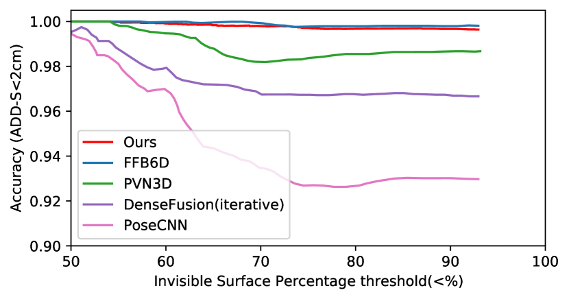
Figure 4: Performance of difference approaches under increasing level of occlusion on YCB-Video Dataset. Our per-RoI method is effective at identifying and handling occlusion.

4.3 Quantitative Comparison with Other Methods

We compare the proposed method with others on YCB-Video, LineMOD, and Occlusion LineMOD datasets. Experimental results of YCB-Video dataset are reported in main paper and the results of LineMOD and Occlusion LineMOD are in Appendix.

Evaluation results on YCB-Video dataset. We report the quantitative results of the proposed Uni6D on YCB-Video dataset in Table 1. In comparison to other methods, our approach achieves 95.2% on the ADD-S metric and 88.8% on the ADD(S) metric with a succinct and straightforward pipeline. Although the previous method DenseFusion [11] does not use post-processing like our method, our method improves the ADD-S by 4%. In contrast to DenseFusion, which requires two different backbones, CNN and PointNet [14], our method only needs a unified CNN to extract RGB-D features. It is worth emphasizing that although the performance of our method is a little bit lower than the current state-of-the-art methods [6, 16], it does not use any additional iterative refinement and post-process operations which are required in state-of-the-art methods. We discuss the time efficiency of our method below. Following [11, 16], we also evaluate the robustness towards occlusion in YCB-Video dataset through calculating how the accuracy ($\textrm{ADD-S}<2$cm) changes with extent of occlusion. As indicated in Fig. 4, the performances of our methods has the minimal drop compared with DenseFusion [11] and FFB6D [16]. In particular, the performance under increasing level of occlusion decrease by 0.3%, which is comparable to FFB6D. Occlusion should be better identified and handled because our RT prediction is based on a RoI.

Table 2: Time cost and frames per second (FPS) on YCB-Video Dataset. Our Uni6D is $7.2\times$ faster than FFB6D, and $13.6\times$ than PVN3D. It is capable of estimating 6D pose in real-time. Note that the results of PoseCNN and DenseFusion comes from [11], which does not state their device type.

Method	Network	Post-process	ALL	FPS
PoseCNN+ICP [53]	200	10400	10600	0.094
PoseCNN [53]	200	0	200	5
DenseFusion [11]	50	10	60	16.67
PVN3D [6]	110	420	530	1.89
FFB6D [16]	20	260	280	3.57
Ours	39	0	39	25.64

Time efficiency. To highlight the inference efficiency of our straightforward pipeline, we compare the inference speed of our method with PoseCNN+ICP [53], PoseCNN [53], DenseFusion [11], PVN3D [6] and FFB6D [16] in Table 2. Post-processing accounts for 92.9% of the total time in FFB6D and 79.2% in PVN3D. DenseFusion has a faster inference speed compares to them, while our method further speeds up the inference, benefited from our straightforward pipeline which does not need any post-processing. Our Uni6D is $7.2\times$ faster than FFB6D, and $13.6\times$ than PVN3D. Comparison results of inference time and performance are shown in Fig 5.

4.4 Implementation Details

In all experiments, we adopt ResNet-50 [49] as the backbone network with FPN [50]. We train all models with 16 GPUs (three images per GPU) for 40 epochs with an SGD optimizer which momentum is 0.9 and weight-decay is 0.0001. The initial learning rate is set to 0.0075 with a linear warm-up, and decreased by 0.1 after 15, 25 and 35 epochs. The weight hyperparameter $\lambda_{0}$ in the loss function of RT head is set to 1 in epoch $[1,20)$, 5 in $[20,30)$, 20 in $[30,38)$ and 50 in $[38,40]$.

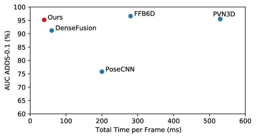
Figure 5: Balance the simplicity/speed and accuracy.

4.5 Ablation Study

4.5.1 Projection Breakdown Saved by UV

To investigate the effects of the UV encoding information in the projection breakdown problem, we perform experiments with several spatial transformations on the YCB-Video dataset in Table 3. Using any of the common spatial transformations as training augmentation methods, such as random resize, crop, horizontal flip, and vertical flip, significantly reduces performance by up to 15% ADD-S and 20% ADD(S). These results directly reflect the destructiveness of projection breakdown. We add explicit UV encoding information with UV, XY, and PE to solve this issue and make the one backbone is all you need possible.

4.5.2 UV Encoding Methods

We investigate the contributions of all components in UV encoding of our method on the YCB-Video dataset. The results are shown in Table 4. “RGB-D” denotes that we only use RGB-D data as input, which is used as the baseline. “Plain UV” means the plain UV coordinates data. “XY” represents adding the inverse projected XY coordinates data. “NRM” means the depth normal vector. “PE” is the position encoding. “abc head” denotes adding the abc head during training. We can see that the flip transformation degrades performance in the baseline, and that adding position information to the RGB-D data in the form of plain UV, XY, NRM, or PE can alleviate this degradation. Compared with the baseline, our method brings 4.19% improvement in ADD-S and 9.11% in ADD(S).

Table 3: Effects of the UV encoding under varying spatial transformations. Spatial transformations greatly harm the accuracy when no UV encoding information is provided, but improve the accuracy with UV encoding information.

UV Enc	Resize	Crop	Hflip	Vflip	ADD-S	ADD(S)
w/o	✓	✓	✓	✓	78.87	65.88
w	✓	✓	✓	✓	92.82	81.95
w/o	✓	✓	✓		79.01	65.79
w	✓	✓	✓		93.61	84.36
w/o	✓	✓		✓	90.40	79.26
w	✓	✓		✓	93.18	84.31
w/o	✓				92.92	83.39
w	✓				93.89	85.76
w/o		✓			92.45	83.18
w		✓			92.96	85.05

4.6 Qualitative Results

For intuitively comparing the qualitative results between our Uni6D and other methods [6, 16] on the YCB-Video dataset, we give some estimation results in Fig. 6. Our Uni6D significantly outperforms the state of the art and performs the most robust in different occlusion situations.

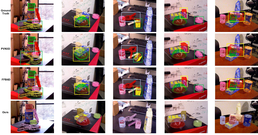
Figure 6: Qualitative results of 6D pose on the YCB-Video dataset.

5 Limitation Analysis

In this section, we discuss the limitations of our method.

For the performance of 6D pose estimation, our method still has a little gap compared with the state of the art in YCB dataset. The main reason is that we do not use any time-consuming post-processing or iteration refinement in the pipeline of our method. We only add a lightweight abc head with the abc regression task to introduce an auxiliary loss for auxiliary model training. In inference, the abc head is removed and we directly obtain the 6D pose estimation results from the RT head. This straightforward inference pipeline significantly improves the efficiency of inference and reduces the difficulty of engineering implementation. It is worth exploring more efficient post-processing algorithms for our unified 2D CNN to further improve the performance while maintaining real-time inference.

For the RoI-Align operation, it limits the performance of RT head and reduces the accuracy of our method. The training and testing of our end-to-end method is applied in a RoI-wise manner with a rough object-level feature for each object, which is different from the per-pixel dense prediction widely used in previous works [53, 11, 16]. More research into de-noising RoI features for better results without sacrificing simplicity is needed.

Table 4: Effects of each component in our work. Results of ADD(S) AUC and ADD-S AUC on YCB-Video are reported respectively. Compared with the baseline, our method brings 4.19% improvement in ADD-S and 9.11% in ADD(S).

RGB-D	Plain UV	XY	PE	NRM	abc head	ADD-S	ADD(S)
✓						90.99	79.72
✓	✓					94.06	85.39
✓		✓				94.17	85.66
✓			✓			93.54	85.05
✓				✓		93.79	84.79
✓	✓	✓				93.90	85.06
✓		✓	✓			93.27	84.49
✓	✓		✓			93.65	84.51
✓		✓		✓		94.70	86.76
✓	✓			✓		94.26	85.52
✓			✓	✓		93.31	83.42
✓	✓	✓	✓			93.55	84.83
✓	✓	✓	✓	✓		94.91	86.93
✓	✓	✓	✓	✓	✓	95.18	88.83

6 Conclusions

In this paper, we reveal the “projection breakdown” hidden underneath CNN-based depth image processing, which explains the two-backbone design for RGB-D processing and the per-pixel feature extraction for depth processing adopted by most of the existing literature. Rather than using two separate backbones, we fix the projection breakdown by explicitly feeding extra UV data along with depth to the backbone. As a result, all you need to extract the feature from RGB-D images is a general 2D CNN backbone. Thus, we propose Uni6D, an end-to-end 6D pose estimation framework based on Mask R-CNN. Uni6D uses ResNet and FPN as its backbone to extract features from RGB-D images, extra feature fusion is not required anymore. The 6D pose estimation results are obtained directly from the RT head using a straightforward inference pipeline that does not require any time-consuming post-processing. We also develop the abc head as an auxiliary task for training the network in our framework. Extensive experimental results show our method outperforms other state-of-the-art methods in terms of time efficiency, performance, and robustness in the challenging YCB-Video. Worthwhile and related future work can be spawned from the proposed new 6D pose estimation paradigm, which performs 6D pose estimation with a unified CNN framework with the above contributions.

Supplementary Material for
Uni6D: A Unified CNN Framework without Projection Breakdown for 6D Pose Estimation

7 More implementation details

7.1 The details of the positional encoding.

PE is implemented using equation 7 and the details will be added in the final version.

$$PE(x,y,2i)=sin(x/10000^{(4i/D)})$$ (7)

$$PE(x,y,2i+1)=cos(x/10000^{(4i/D)})$$

$$PE(x,y,2j+D/2)=sin(y/10000^{(4j/D)})$$

$$PE(x,y,2j+1+D/2)=cos(y/10000^{(4j/D)}),$$

where $(x,y)$ is a point in 2d space, $i,j$ is an integer in $[0,D/4)$, $D$ is the size of the channel dimension.

7.2 The details of the pre-trained weight.

We use the ImageNet pre-trained weight, and the first convolutional layer is initialized with the kaiming uniform. For YCB dataset:

• Backbone: ResNet50 + FPN;

• Input data: RGB-D+UV+PE+XY+NRM, rotation matrices are represented by quaternions, other settings are same with PVN3D [6];

• Data augmentation:

  1. multi-scale training: [320, 400, 480, 600, 720] (max size is 900);

  2. background replacing: replace the background of the rendered data with the real image background;

  3. random crop: 0.3 probability, need to keep all objects;

• Training:

  1. Pretrained: ImageNet;

  2. Schedule: 40epoch, MultiStepLR with [15, 25, 35] schedule and 0.1$\times$ decay ;

  3. Optimizer: SGD, momentum 0.9, weight_deacy 0.0001, warm-up 4 epoch;

• Loss function:

  1. $\mathcal{L}=\lambda_{0}\cdot\mathcal{L}_{rt}+\mathcal{L}_{abc}+\mathcal{L}_{mask}+\mathcal{L}_{bbox}+\mathcal{L}_{cls}+\mathcal{L}_{rpn}$

  2. $\lambda_{0}$ is changed in training: 1-15 epoch is 1, 16-25 epoch is 5, 26-35 epoch is 10 and 36-40 epoch is 20;

For Linemode dataset:

• Backbone: ResNet50 + FPN;

• Input data: RGB-D+UV+PE+XY+NRM, rotation matrices are represented by quaternions, other settings are same with PVN3D [6], except using camera intrinsics for real data to render data;

• Data augmentation:

  1. multi-scale training: [320, 400, 480, 600, 720] (max size is 900);

  2. background replacing: replace the background of the rendered data with the real image background;

  3. random crop: 0.3 probability, need to keep all objects;

  4. random erase: 0.1 probability

• Training:

  1. Pretrained: ImageNet;

  2. Schedule: 40epoch, MultiStepLR with [15, 25, 35] schedule and 0.1$\times$ decay ;

  3. Optimizer: SGD, momentum 0.9, weight_deacy 0.0001, warm-up 4 epoch;

• Loss function:

  1. $\mathcal{L}=\lambda_{0}\cdot\mathcal{L}_{rt}+\mathcal{L}_{abc}+\mathcal{L}_{mask}+\mathcal{L}_{bbox}+\mathcal{L}_{cls}+\mathcal{L}_{rpn}$

  2. $\lambda_{0}$ is changed in training: 1-15 epoch is 1, 16-25 epoch is 5, 26-35 epoch is 10 and 36-40 epoch is 20;

8 Ablation Studies of abc Head

We provide results of more ablation studies for abc head on YCB dataset in Table 5. We combine the abc head with different UV input information to verify the effectiveness of it. We can observe that our abc head can improve the performance without UV and it can further improve the performance with different types of UV. These results demonstrate the effectiveness of abc head as an auxiliary training task.

	RGB-D	Plain UV	XY	PE	NRM
w/o	90.99/79.72	94.06/85.39	94.17/85.66	93.54/85.05	93.79/84.79
w	91.13/80.89	94.49/86.46	94.33/86.90	93.53/86.09	93.89/84.96

Table 5: Ablation study results of abc head, the format is ADDS/ADD(S).

9 Quantitative Results on the LineMOD Dataset

Experimental results of LineMOD dataset are reported in Table 6, our approach achieves 97.03% ADD-0.1d ACC with a succinct and straightforward pipeline compared with other methods. LineMOD is usually thought to be less challenging due to the varying lighting conditions, significant image noise and occlusions in YCB-Video Dataset.

Table 6: Evaluation results (ADD-0.1d ACC) on the LineMOD dataset. Symmetric objects are denoted in bold.

	PoseCNN [53]	PVNet [30]	CDPN [36]	DOPD [54]	PointFusion [2]	DenseFusion [11]	G2L-Net [55]	PVN3D [6]	FFB6D [16]	Our Uni6D
ape	77.0	43.6	64.4	87.7	70.4	92.3	96.8	97.3	98.4	93.71
benchvise	97.5	99.9	97.8	98.5	80.7	93.2	96.1	99.7	100.0	99.81
camera	93.5	86.9	91.7	96.1	60.8	94.4	98.2	99.6	99.9	95.98
can	96.5	95.5	95.9	99.7	61.1	93.1	98.0	99.5	99.8	99.02
cat	82.1	79.3	83.8	94.7	79.1	96.5	99.2	99.8	99.9	98.10
driller	95.0	96.4	96.2	98.8	47.3	87.0	99.8	99.3	100.0	99.11
duck	77.7	52.6	66.8	86.3	63.0	92.3	97.7	98.2	98.4	89.95
eggbox	97.1	99.2	99.7	99.9	99.9	99.8	100.0	99.8	100.0	100.00
glue	99.4	95.7	99.6	96.8	99.3	100.0	100.0	100.0	100.0	99.23
holepuncher	52.8	82.0	85.8	86.9	71.8	92.1	99.0	99.9	99.8	90.20
iron	98.3	98.9	97.9	100.0	83.2	97.0	99.3	99.7	99.9	99.49
lamp	97.5	99.3	97.9	96.8	62.3	95.3	99.5	99.8	99.9	99.42
phone	87.7	92.4	90.8	94.7	78.8	92.8	98.9	99.5	99.7	97.41
Avg	88.6	86.3	89.9	95.2	73.7	94.3	98.7	99.4	99.7	97.03

10 Quantitative Results on the Occlusion LineMOD dataset

We follow the previous works [11, 16] to train our model on the LineMOD dataset and only use this dataset for testing. Experimental results of LineMOD dataset are reported in Table 7, and we obtain 30.71 ADDS-0.1d AUC.

Table 7: Evaluation results (ADD-0.1d ACC) on the Occlusion-LineMOD dataset. Symmetric objects are denoted in bold.

Method	PoseCNN [53]	Oberweger [29]	Pix2Pose [56]	PVNet [30]	DPOD [54]	Hu [57]	HybridPose [58]	PVN3D [6]	FFB6D [16]	Our Uni6D
ape	9.6	12.1	22.0	15.8	-	19.2	20.9	33.9	47.2	32.99
can	45.2	39.9	44.7	63.3	-	65.1	75.3	88.6	85.2	51.04
cat	0.9	8.2	22.7	16.7	-	18.9	24.9	39.1	45.7	4.56
driller	41.4	45.2	44.7	65.7	-	69.0	70.2	78.4	81.4	58.40
duck	19.6	17.2	15.0	25.2	-	25.3	27.9	41.9	53.9	34.80
eggbox	22.0	22.1	25.2	50.2	-	52.0	52.4	80.9	70.2	1.73
glue	38.5	35.8	32.4	49.6	-	51.4	53.8	68.1	60.1	30.16
holepuncher	22.1	36.0	49.5	39.7	-	45.6	54.2	74.7	85.9	32.07
Avg	24.9	27.0	32.0	40.8	47.3	43.3	47.5	63.2	66.2	30.71

11 More Qualitative Results

We give more qualitative comparison results between our method and the SOTA method FFB6D [16] in Fig. 7 for YCB-Video dataset and Fig. 8 for LineMOD dataset. Moreover, We strongly recommend readers to watch the video from https://youtu.be/6G__P282djw , which directly reflects the comparison results between our method and the FFB6D [16]. Compared with FFB6D, our method estimates the 6d pose more smoothly. Our method has better consistency between adjacent frames, less jitter, and more robust performance under severe occlusion conditions.

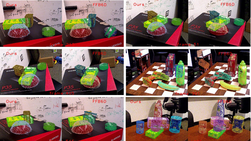
Figure 7: Qualitative results of 6D pose on the YCB-Video dataset. In each sub-figure, left is the result of our method and the right is of the SOTA method FFB6D [16].

Figure 8: Qualitative results of 6D pose on the LineMOD dataset.

References

- [1] Andreas Geiger, Philip Lenz, and Raquel Urtasun. Are we ready for autonomous driving? the kitti vision benchmark suite. In 2012 IEEE conference on computer vision and pattern recognition, pages 3354–3361. IEEE, 2012.
- [2] Danfei Xu, Dragomir Anguelov, and Ashesh Jain. Pointfusion: Deep sensor fusion for 3d bounding box estimation. In Proceedings of the IEEE conference on computer vision and pattern recognition, pages 244–253, 2018.
- [3] Xiaozhi Chen, Huimin Ma, Ji Wan, Bo Li, and Tian Xia. Multi-view 3d object detection network for autonomous driving. In Proceedings of the IEEE conference on Computer Vision and Pattern Recognition, pages 1907–1915, 2017.
- [4] Alvaro Collet, Manuel Martinez, and Siddhartha S Srinivasa. The moped framework: Object recognition and pose estimation for manipulation. The international journal of robotics research, 30(10):1284–1306, 2011.
- [5] Jonathan Tremblay, Thang To, Balakumar Sundaralingam, Yu Xiang, Dieter Fox, and Stan Birchfield. Deep object pose estimation for semantic robotic grasping of household objects. In Conference on Robot Learning, pages 306–316. PMLR, 2018.
- [6] Yisheng He, Wei Sun, Haibin Huang, Jianran Liu, Haoqiang Fan, and Jian Sun. Pvn3d: A deep point-wise 3d keypoints voting network for 6dof pose estimation. In IEEE/CVF Conference on Computer Vision and Pattern Recognition (CVPR), June 2020.
- [7] Eric Marchand, Hideaki Uchiyama, and Fabien Spindler. Pose estimation for augmented reality: a hands-on survey. IEEE transactions on visualization and computer graphics, 22(12):2633–2651, 2015.
- [8] Kaiming He, Georgia Gkioxari, Piotr Dollár, and Ross Girshick. Mask r-cnn. In Proceedings of the IEEE international conference on computer vision, pages 2961–2969, 2017.
- [9] Charles R Qi, Wei Liu, Chenxia Wu, Hao Su, and Leonidas J Guibas. Frustum pointnets for 3d object detection from rgb-d data. In Proceedings of the IEEE conference on computer vision and pattern recognition, pages 918–927, 2018.
- [10] Kentaro Wada, Edgar Sucar, Stephen James, Daniel Lenton, and Andrew J Davison. Morefusion: Multi-object reasoning for 6d pose estimation from volumetric fusion. In Proceedings of the IEEE/CVF conference on computer vision and pattern recognition, pages 14540–14549, 2020.
- [11] Chen Wang, Danfei Xu, Yuke Zhu, Roberto Martín-Martín, Cewu Lu, Li Fei-Fei, and Silvio Savarese. Densefusion: 6d object pose estimation by iterative dense fusion. In Proceedings of the IEEE/CVF conference on computer vision and pattern recognition, pages 3343–3352, 2019.
- [12] Guangliang Zhou, Yi Yan, Deming Wang, and Qijun Chen. A novel depth and color feature fusion framework for 6d object pose estimation. IEEE Transactions on Multimedia, 2020.
- [13] Nuno Pereira and Luís A Alexandre. Maskedfusion: Mask-based 6d object pose estimation. In 2020 19th IEEE International Conference on Machine Learning and Applications (ICMLA), pages 71–78. IEEE, 2020.
- [14] Charles R Qi, Hao Su, Kaichun Mo, and Leonidas J Guibas. Pointnet: Deep learning on point sets for 3d classification and segmentation. In Proceedings of the IEEE conference on computer vision and pattern recognition, pages 652–660, 2017.
- [15] Charles Ruizhongtai Qi, Li Yi, Hao Su, and Leonidas J Guibas. Pointnet++: Deep hierarchical feature learning on point sets in a metric space. Advances in neural information processing systems, 30, 2017.
- [16] Yisheng He, Haibin Huang, Haoqiang Fan, Qifeng Chen, and Jian Sun. Ffb6d: A full flow bidirectional fusion network for 6d pose estimation. In IEEE/CVF Conference on Computer Vision and Pattern Recognition (CVPR), June 2021.
- [17] Berk Calli, Arjun Singh, Aaron Walsman, Siddhartha Srinivasa, Pieter Abbeel, and Aaron M Dollar. The ycb object and model set: Towards common benchmarks for manipulation research. In 2015 international conference on advanced robotics (ICAR), pages 510–517. IEEE, 2015.
- [18] Daniel P Huttenlocher, Gregory A. Klanderman, and William J Rucklidge. Comparing images using the hausdorff distance. IEEE Transactions on pattern analysis and machine intelligence, 15(9):850–863, 1993.
- [19] Chunhui Gu and Xiaofeng Ren. Discriminative mixture-of-templates for viewpoint classification. In European Conference on Computer Vision, pages 408–421. Springer, 2010.
- [20] Stefan Hinterstoisser, Cedric Cagniart, Slobodan Ilic, Peter Sturm, Nassir Navab, Pascal Fua, and Vincent Lepetit. Gradient response maps for real-time detection of textureless objects. IEEE transactions on pattern analysis and machine intelligence, 34(5):876–888, 2011.
- [21] Yu Xiang, Tanner Schmidt, Venkatraman Narayanan, and Dieter Fox. Posecnn: A convolutional neural network for 6d object pose estimation in cluttered scenes. arXiv preprint arXiv:1711.00199, 2017.
- [22] Yi Li, Gu Wang, Xiangyang Ji, Yu Xiang, and Dieter Fox. Deepim: Deep iterative matching for 6d pose estimation. In Proceedings of the European Conference on Computer Vision (ECCV), pages 683–698, 2018.
- [23] Shubham Tulsiani and Jitendra Malik. Viewpoints and keypoints. In Proceedings of the IEEE Conference on Computer Vision and Pattern Recognition, pages 1510–1519, 2015.
- [24] Hao Su, Charles R Qi, Yangyan Li, and Leonidas J Guibas. Render for cnn: Viewpoint estimation in images using cnns trained with rendered 3d model views. In Proceedings of the IEEE International Conference on Computer Vision, pages 2686–2694, 2015.
- [25] Martin Sundermeyer, Zoltan-Csaba Marton, Maximilian Durner, Manuel Brucker, and Rudolph Triebel. Implicit 3d orientation learning for 6d object detection from rgb images. In Proceedings of the European Conference on Computer Vision (ECCV), pages 699–715, 2018.
- [26] Keunhong Park, Arsalan Mousavian, Yu Xiang, and Dieter Fox. Latentfusion: End-to-end differentiable reconstruction and rendering for unseen object pose estimation. In Proceedings of the IEEE/CVF conference on computer vision and pattern recognition, pages 10710–10719, 2020.
- [27] Fred Rothganger, Svetlana Lazebnik, Cordelia Schmid, and Jean Ponce. 3d object modeling and recognition using local affine-invariant image descriptors and multi-view spatial constraints. International journal of computer vision, 66(3):231–259, 2006.
- [28] Alex Kendall, Matthew Grimes, and Roberto Cipolla. Posenet: A convolutional network for real-time 6-dof camera relocalization. In Proceedings of the IEEE international conference on computer vision, pages 2938–2946, 2015.
- [29] Markus Oberweger, Mahdi Rad, and Vincent Lepetit. Making deep heatmaps robust to partial occlusions for 3d object pose estimation. In Proceedings of the European Conference on Computer Vision (ECCV), pages 119–134, 2018.
- [30] Sida Peng, Yuan Liu, Qixing Huang, Xiaowei Zhou, and Hujun Bao. Pvnet: Pixel-wise voting network for 6dof pose estimation. In Proceedings of the IEEE/CVF Conference on Computer Vision and Pattern Recognition, pages 4561–4570, 2019.
- [31] Xingyu Liu, Rico Jonschkowski, Anelia Angelova, and Kurt Konolige. Keypose: Multi-view 3d labeling and keypoint estimation for transparent objects. In Proceedings of the IEEE/CVF conference on computer vision and pattern recognition, pages 11602–11610, 2020.
- [32] Daniel Glasner, Meirav Galun, Sharon Alpert, Ronen Basri, and Gregory Shakhnarovich. Aware object detection and pose estimation. In 2011 International Conference on Computer Vision, pages 1275–1282. IEEE, 2011.
- [33] Eric Brachmann, Alexander Krull, Frank Michel, Stefan Gumhold, Jamie Shotton, and Carsten Rother. Learning 6d object pose estimation using 3d object coordinates. In European conference on computer vision, pages 536–551. Springer, 2014.
- [34] Wadim Kehl, Fausto Milletari, Federico Tombari, Slobodan Ilic, and Nassir Navab. Deep learning of local rgb-d patches for 3d object detection and 6d pose estimation. In European conference on computer vision, pages 205–220. Springer, 2016.
- [35] Andreas Doumanoglou, Rigas Kouskouridas, Sotiris Malassiotis, and Tae-Kyun Kim. Recovering 6d object pose and predicting next-best-view in the crowd. In Proceedings of the IEEE conference on computer vision and pattern recognition, pages 3583–3592, 2016.
- [36] Zhigang Li, Gu Wang, and Xiangyang Ji. Cdpn: Coordinates-based disentangled pose network for real-time rgb-based 6-dof object pose estimation. In Proceedings of the IEEE/CVF International Conference on Computer Vision, pages 7678–7687, 2019.
- [37] He Wang, Srinath Sridhar, Jingwei Huang, Julien Valentin, Shuran Song, and Leonidas J Guibas. Normalized object coordinate space for category-level 6d object pose and size estimation. In Proceedings of the IEEE/CVF Conference on Computer Vision and Pattern Recognition, pages 2642–2651, 2019.
- [38] Dengsheng Chen, Jun Li, Zheng Wang, and Kai Xu. Learning canonical shape space for category-level 6d object pose and size estimation. In Proceedings of the IEEE/CVF conference on computer vision and pattern recognition, pages 11973–11982, 2020.
- [39] Tomas Hodan, Daniel Barath, and Jiri Matas. Epos: Estimating 6d pose of objects with symmetries. In Proceedings of the IEEE/CVF conference on computer vision and pattern recognition, pages 11703–11712, 2020.
- [40] Ming Cai and Ian Reid. Reconstruct locally, localize globally: A model free method for object pose estimation. In Proceedings of the IEEE/CVF Conference on Computer Vision and Pattern Recognition, pages 3153–3163, 2020.
- [41] Shuran Song and Jianxiong Xiao. Sliding shapes for 3d object detection in depth images. In European conference on computer vision, pages 634–651. Springer, 2014.
- [42] Shuran Song and Jianxiong Xiao. Deep sliding shapes for amodal 3d object detection in rgb-d images. In Proceedings of the IEEE conference on computer vision and pattern recognition, pages 808–816, 2016.
- [43] Yin Zhou and Oncel Tuzel. Voxelnet: End-to-end learning for point cloud based 3d object detection. In Proceedings of the IEEE conference on computer vision and pattern recognition, pages 4490–4499, 2018.
- [44] Stefan Hinterstoisser, Stefan Holzer, Cedric Cagniart, Slobodan Ilic, Kurt Konolige, Nassir Navab, and Vincent Lepetit. Multimodal templates for real-time detection of texture-less objects in heavily cluttered scenes. In 2011 international conference on computer vision, pages 858–865. IEEE, 2011.
- [45] Stefan Hinterstoisser, Vincent Lepetit, Slobodan Ilic, Stefan Holzer, Gary Bradski, Kurt Konolige, and Nassir Navab. Model based training, detection and pose estimation of texture-less 3d objects in heavily cluttered scenes. In Asian conference on computer vision, pages 548–562. Springer, 2012.
- [46] Reyes Rios-Cabrera and Tinne Tuytelaars. Discriminatively trained templates for 3d object detection: A real time scalable approach. In Proceedings of the IEEE international conference on computer vision, pages 2048–2055, 2013.
- [47] Alykhan Tejani, Danhang Tang, Rigas Kouskouridas, and Tae-Kyun Kim. Latent-class hough forests for 3d object detection and pose estimation. In European Conference on Computer Vision, pages 462–477. Springer, 2014.
- [48] Paul Wohlhart and Vincent Lepetit. Learning descriptors for object recognition and 3d pose estimation. In Proceedings of the IEEE conference on computer vision and pattern recognition, pages 3109–3118, 2015.
- [49] Kaiming He, Xiangyu Zhang, Shaoqing Ren, and Jian Sun. Deep residual learning for image recognition. In Proceedings of the IEEE conference on computer vision and pattern recognition, pages 770–778, 2016.
- [50] Tsung-Yi Lin, Piotr Dollár, Ross Girshick, Kaiming He, Bharath Hariharan, and Serge Belongie. Feature pyramid networks for object detection. In Proceedings of the IEEE conference on computer vision and pattern recognition, pages 2117–2125, 2017.
- [51] Sho Takase and Naoaki Okazaki. Positional encoding to control output sequence length. In Proceedings of the 2019 Conference of the North American Chapter of the Association for Computational Linguistics: Human Language Technologies, Volume 1 (Long and Short Papers), pages 3999–4004, 2019.
- [52] Ashish Vaswani, Noam Shazeer, Niki Parmar, Jakob Uszkoreit, Llion Jones, Aidan N Gomez, Łukasz Kaiser, and Illia Polosukhin. Attention is all you need. In Advances in neural information processing systems, pages 5998–6008, 2017.
- [53] Yu Xiang, Tanner Schmidt, Venkatraman Narayanan, and Dieter Fox. Posecnn: A convolutional neural network for 6d object pose estimation in cluttered scenes. 2018.
- [54] Sergey Zakharov, Ivan Shugurov, and Slobodan Ilic. Dpod: 6d pose object detector and refiner. In Proceedings of the IEEE/CVF International Conference on Computer Vision, pages 1941–1950, 2019.
- [55] Wei Chen, Xi Jia, Hyung Jin Chang, Jinming Duan, and Ales Leonardis. G2l-net: Global to local network for real-time 6d pose estimation with embedding vector features. In Proceedings of the IEEE/CVF conference on computer vision and pattern recognition, pages 4233–4242, 2020.
- [56] P Kiru, Timothy Patten, and MV Pix2Pose. Pixel-wise coordinate regression of objects for 6d pose estimation. Proceedings of the ICCV, Seoul, Korea, pages 27–28, 2019.
- [57] Yinlin Hu, Pascal Fua, Wei Wang, and Mathieu Salzmann. Single-stage 6d object pose estimation. In Proceedings of the IEEE/CVF conference on computer vision and pattern recognition, pages 2930–2939, 2020.
- [58] Chen Song, Jiaru Song, and Qixing Huang. Hybridpose: 6d object pose estimation under hybrid representations. In Proceedings of the IEEE/CVF conference on computer vision and pattern recognition, pages 431–440, 2020.