Spontaneous scalarization in (A)dS gravity
at zero temperature

Alessio Marrani¹, Olivera Miskovic², and Paula Quezada Leon²

¹Instituto de Física Teorica, Dep.to de Física,
Universidad de Murcia, Campus de Espinardo, E-30100, Spain
jazzphyzz@gmail.com

²Instituto de Física, Pontificia Universidad Católica de Valparaíso,
Casilla 4059, Valparaíso, Chile
olivera.miskovic@pucv.cl
pquezada.l@gmail.com

We study spontaneous scalarization of electrically charged extremal black holes in $D\geq 4$ spacetime dimensions. Such a phenomenon is caused by the symmetry breaking due to quartic interactions of the scalar – Higgs potential and Stueckelberg interaction with electromagnetic and gravitational fields, characterized by the couplings $a$ and $b$, respectively. We use the entropy representation of the states in the vicinity of the horizon, apply the inverse attractor mechanism for the scalar field, and analyze analytically the thermodynamic stability of the system using the laws of thermodynamics. As a result, we obtain that the scalar field condensates on the horizon only in spacetimes which are asymptotically non-flat, $\Lambda\neq 0$ (dS or AdS), and whose extremal black holes have non-planar horizons $k=\pm 1$, provided that the mass $m$ of the scalar field belongs to a mass interval (area code) different for each set of the boundary conditions specified by $(\Lambda,k)$. A process of scalarization describes a second order phase transition of the black hole, from the extremal Reissner-Nordström (A)dS one, to the corresponding extremal hairy one. Furthermore, for the transition to happen, the interaction has to be strong enough, and all physical quantities on the horizon depend at most on the effective Higgs-Stueckelberg interaction $am^{2}-2b$. Most of our results are general, valid for any parameter and any spacetime dimension.

1 Introduction

The no-hair theorem, holding in Einstein-Maxwell theories [1, 2, 3], states that a black hole (BH) in four-dimensional asymptotically flat spacetime is determined in a unique way in terms of three physical parameters, namely by its mass $M$, electric charge $Q$ and angular momentum $J$; in other words, all higher BH multipole moments are determined only by $M$, $Q$ and $J$. More properly, such a theorem should be referred to as “no-independent-multipole-hair” theorem: higher gravitational multipole moments – quadrupole and higher – (and electromagnetic multipole moments – dipole and higher) are not independent for Kerr-Newman BHs. Moreover, the expectation of astrophysical BHs being with no electric charge yields to reasonably conjecture that, in presence of any type of matter-energy, the class of Kerr BHs is the end point of gravitational collapse and thus the most realistic class of solutions to Maxwell-Einstein equations, being uniquely characterized by $M$ and $J$, with no hair whatsoever (this is the so-called “Kerr hypothesis”). Current and future observations [4] are testing this conjecture, which has so far been confirmed in various ways, e.g., by the motion of stars around the supermassive BH at the center of the Milky Way (2020 Nobel Prize), by the observation of gravitational waves from BH mergers (2017 Nobel Prize), and by the observation of the shadow of the supermassive BH at the center of M87 (EHT collaboration).

However, throughout the years, stationary BH solutions, usually referred to as ‘hairy BHs’, with either new global charges (primary hair) or new non-trivial fields not associated to a Gauss law – even if not independent from the standard global charges (secondary hair) – have been found in a number of contexts, in which one or more assumptions underlying the aforementioned no-hair theorem were violated.

In fact, by allowing for more general –nonminimal– coupling functions of the scalar fields to gravity and electromagnetic fields in the Lagrangian density, a new interesting phenomenon, dubbed “spontaneous scalarization”, was observed: namely, the destabilization of scalar-free BH solutions and the arising of scalar hair. This typically occurs in a number of theories characterized by a non-minimal coupling of the scalar fields themselves, such that, at critical values of the coupling, BHs develop a tachyonic instability, and new branches of spontaneously scalarized BHs arise out. Neutron stars in scalar-tensor models in which scalar fields were coupled to the Ricci curvature have been the first framework in which scalarization was observed [5]. Since then, such a phenomenon has been established to occur in a number of contexts, e.g., when BHs are coupled to non-linear electrodynamics [6, 7], or surrounded by non-conformally invariant matter [8, 9], or in Einstein-Yang-Mills theory [10, 11, 12], Skyrme hairy black holes [13, 14], and black holes with dilatonic hair [15] (see [16], and e.g. [17] for a review on asymptotically flat BHs). The first example of scalarization with a conformally coupled scalar field $\frac{1}{6}\phi^{2}R$ in four dimensions has been discussed in [18, 19]. In general, fast rotation of the black hole can induce a tachyonic instability when the scalar is suitably coupled to the curvature [20].

On the other hand, BH scalarization can also be induced by higher curvature term corrections to Einstein gravity, coupled to the scalar fields. Furthermore, when the cosmological constant is negative, $\Lambda<0$, the Reissner-Nordström (RN) BH is not unique in four dimensions, and there are also other static BHs of Einstein-Maxwell gravity that have no continuous spatial symmetries; their horizons are smooth and topologically spherical, and they form bound states with the AdS soliton possessing an arbitrary multipole structure [21, 22]. In recent years, a number of studies [23]–[30] has investigated asymptotically anti-de-Sitter (AdS) spontaneously scalarized BHs, in which scalar fields are non-minimally couples to the Ricci scalar and Gauss-Bonnet term [31], also in higher dimensions [32]. In particular, the spontaneous scalarization phenomenon is also present in the spinning black holes in the Einstein-Gauss-Bonnet-scalar theory [33].

Either due to the existence of gravitating solitons, or due to the existence of some particular scalar-gravity couplings, there is now tantamount evidence that, notwithstanding scalar fields usually do not enjoy a Gauss-like law and consequently are hard to keep in equilibrium with an event horizon without trivializing, BH solutions with scalar hair, aka hairy BHs, exist nevertheless.

At any rate, in presence of non-linear and/or higher-derivative curvature terms, the equations of motion are hard to be solved in analytical way, and only numerical solutions are currently available. This has quite recently motivated the study of the dynamics of scalarized BHs in the simpler class of Einstein–Maxwell-scalar theories with non-minimal couplings between the scalar and Maxwell fields [22], which allows to analytically solve the equations of motion, describing the scalar flow in an intrinsically non-linear way [34, 35]. Various non-minimal coupling functions [36, 37] have been considered, as well as dyons including magnetic charges [38], axionic-type couplings [39], and massive and self-interacting scalar fields [40]–[43]. Spontaneous scalarization was also discussed in presence of a positive cosmological constant [44], as well.

On the other hand, the scalarization that occurs spontaneously in non-extremal BHs in AdS space is an important phenomenon in the context of the gauge/gravity duality, since its dual is provided by holographic superconductor-like systems at constant temperature [45, 46, 47]. A zero-temperature superconductor/insulator phase transition has been obtained in [48] through a mapping of the BH to the AdS soliton, such that the scalar field condensation occurs in the AdS soliton background. In this work, however, we are interested in different settings, namely, in a scalarization of the extremal BH. Such a zero-temperature system has a degenerate ground state with non-vanishing entropy, similarly to spin glasses, which have been of particular interest recently in condensed matter physics due to their intriguing properties (2021 Nobel Prize).

Within this venue of investigation, in [49] zero temperature phase transitions driven by the electric charge of asymptotically AdS extremal BHs in four space-time dimensions were investigated, by exploiting the complex Stueckelberg scalar field as an order parameter. Moreover, it was analytically shown in [49] that the (necessarily massive) scalar field can couple to a RN BH in the extremal limit of vanishing Hawking temperature, but only if the magnetic charge vanishes, and if space-time has a non-zero cosmological constant, and if a non-minimal coupling to gravity is present; in particular, in such a framework asymptotically AdS₄ BHs admit only spherical and hyperbolic near-horizon geometries.

The aforementioned BH scalarization consists of a spontaneous generation of a scalar field $\Psi$ (through symmetry breaking) around the horizon of a BH in a generic class of theories, which may be described by the Lagrangian density

$$\mathcal{L}_{\mathrm{scalarization}}=\frac{1}{2\varkappa}\,R-\frac{1}{2}\,\left(D_{\mu}\Psi\right)^{2}-\frac{1}{2}\,m^{2}\Psi^{2}+P(\Psi)\,\mathcal{I}(g,A)\,,\quad 2\varkappa=16\pi G_{\mathrm{N}}\,,$$ (1.1)

where $P(\Psi)\geq 0$ is at least quadratic in $\Psi,$ and $\mathcal{I}(g,A)$ is any other function of the matter fields (in our particular case, of the electromagnetic field) and the metric. This interaction between the scalar, gravity and electromagnetic field leads to the tachyonic scalar (with $m_{\mathrm{eff}}^{2}<0$) and therefore to spontaneous scalarization. In our case, the matter field appears in a $U(1)$-invariant combination,

$$\mathcal{I}(g,A,\sigma)=\left(\partial\sigma-A\right)^{2}\,,$$ (1.2)

and, in the non-extremal case, it needs at least the term $P(\Psi)=\Psi^{2}$. On the other hand, for the scalarization to occur, one needs that the scalar equation $m^{2}\Psi-f\,\frac{\mathrm{d}P}{\mathrm{d}\Psi}=0$ (where $f$ is the $\Psi$-independent function) possesses at least two different solutions in $\Psi$, and this fact hints at potentials of the form $P\sim\Psi^{n}$ ($n>2$) as natural candidates.

As mentioned above, spontaneous scalarization is usually traced back to a tachyonic instability of the scalar field; however, this may not be necessarily the case. In [51], the appearance of a scalarized RN BH in the Einstein-Maxwell-scalar theory is attributed to the Gregory-Laflamme-like, or modal instability [52], in the sense that it is based on the $\ell=0$ mode perturbations for scalar and tensor fields, and not on a tachyonic field; in other words, the linearized scalar equation of motion includes a non-tachyonic effective mass term which develops negative potential near the horizon from the Maxwell kinetic term. In particular, the coupling $\mathrm{e}^{\alpha\phi^{2}}F^{2}$ has been considered in [51], also pointing out that this exponential potential is very similar to $1+\alpha\phi^{2}$ from the point of view of the bifurcation points in the field equations. The authors performed numerical computations for the scalar field in the background of the RN BH, finding the threshold of the Gregory-Laflamme instability, $\alpha>\alpha_{\mathrm{th}}(q)$.

In [49] and in the present paper, we investigate the spontaneous scalarization of extremal BHs. As discussed in [53] and recalled above, BHs undergo spontaneous scalarization for sufficiently large scalar-tensor couplings $\gamma$, usually attributed to a tachyonic instability of the scalar field system. In the extremal case, a new domain for negative $\gamma$ appears, because of the fact that the near-horizon geometry of a nearly extremal charged black hole is AdS${}_{2}\times\mathbb{S}^{2}$. When the extremal BH is not asymptotically flat (for instance, in the case when $\Lambda<0$), then other geometries can replace $\mathbb{S}^{2}$, such as $\mathbb{R}^{2}$ or $\mathcal{H}^{2}$.

In the present paper, which develops and extends the results of [49], we analytically describe the process of scalarization, exploited via a second order phase transition, from the extremal RN (A)dS BH to the corresponding extremal hairy BH. In order to study phase transitions, a usual thermal field theory approach based on a free energy as an Euclidean continuation of the action is not applicable. Instead, the relevant thermodynamic quantity is the entropy and, to compute it, we apply the entropy function formalism [54, 55]. More explicitly, we are going to discuss thermodynamics of static, electrically charged extremal BHs in Einstein-Maxwell gravity, for any asymptotical behaviour and in presence of a complex scalar field, whose non-minimal couplings are described by the nonlinear Stueckelberg interaction (modifying the kinetic term of the scalar fields) and the Higgs potential. For the scalarization transition to take place, the interactions have to be strong enough; our results show that the scalar field condensates on the unique extremal BH horizon only in presence of a non-vanishing cosmological constant ($\Lambda\neq 0$) and of non-planar near-horizon geometries ($k=\pm 1$), provided that the (necessarily non-vanishing) mass of the scalar field is specified within a suitable interval depending on the boundary conditions specified by $\Lambda$ and $k$.

The plan of the paper is as follows. We introduce the $D$-dimensional Einstein-Maxwell system coupled to a complex scalar field in Sec. 2, where we also present a class of non-minimal interactions of interest. We then derive a set of algebraic equations that govern the entropic behaviour of the system in Sec. 3 where, at the end, we also point out some general features of our treatment. Next, we proceed to solve the equations without the scalar field in different settings in Sec. 4, whereas we discuss non-solvable equations in presence of the scalar field in Sec. 5, finding the critical points of the possible phase transitions. In Sec. 6, we determine the critical exponents for these transitions, and find a near-critical expression for the entropy in Secs. 7 and 8, without and with the scalar field, respectively. Since the equation for the radius of the transversal space strongly depends on the space dimension, in Sec. 9 we focus on the five-dimensional case, providing an interpretation of our results. However, at the end of the section, we highlight several general features valid in any dimension. Finally, we summarize our results and related open questions in Sec. 10.

2 Einstein-Maxwell-scalar systems with $\Lambda\neq 0$

We consider Einstein-Maxwell gravity coupled to one complex scalar field in $D$-dimensional spacetime, in presence of an arbitrary cosmological constant $\Lambda$. The dynamics is described by the action

$$I=\int\mathrm{d}^{D}x\,\sqrt{-g}\,\mathcal{L}=\int\mathrm{d}^{D}x\sqrt{-g}\left(\frac{1}{2\varkappa}\,\left(R-2\Lambda\right)-\frac{1}{4}\,F^{2}+\mathcal{L}_{\mathrm{S}}\right)\,,$$ (2.1)

where $R=g^{\mu\nu}R_{\mu\alpha\nu}^{\alpha}$ is the scalar curvature of the spacetime metric field $g_{\mu\nu}(x)$, $F_{\mu\nu}=\partial_{\mu}A_{\nu}-\partial_{\nu}A_{\mu}$ is the 2-form field strength associated to the vector potential $A_{\mu}(x)$ and $\mathcal{L}_{\mathrm{S}}$ is the scalar field Lagrangian density. We also denote the strength of gravitational interaction by $\varkappa=8\pi G_{\mathrm{N}}$.

The scalar field $\hat{\Psi}=\Psi(x)\mathrm{e}^{\mathrm{i}\sigma(x)}$ is coupled non-minimally to the system through a non-linear Stueckelberg interaction [58]

$$\mathcal{L}_{\mathrm{S}}=-\frac{1}{2}\,\left(\partial\Psi\right)^{2}-\frac{1}{2}\,P(\Psi)\left(\partial\sigma-A\right)^{2}-V(\Psi)\,,\quad P(\Psi)\geq 0\,,$$ (2.2)

often used to describe first and second order phase transitions of non-extremal black holes in Einstein-Maxwell-tensor gravity [47, 50]. The usual minimally coupled scalar Lagrangian $-\frac{1}{2}\,|\partial\hat{\Psi}-\mathrm{i}A\hat{\Psi}|^{2}$ is reproduced in the special case $P(\Psi)=\Psi^{2}$. Note that $\Psi:=|\hat{\Psi}|\geq 0$ and the field $\sigma(x)$ is defined on a compact domain due to an identification $\sigma+2n\pi=\sigma$, $n\in\mathbb{Z}$. The full action is thus invariant under the $U(1)$ gauge symmetry

$$\hat{\Psi}\rightarrow\mathrm{e}^{i\lambda}\hat{\Psi},\qquad A_{\mu}\rightarrow A_{\mu}+\partial_{\mu}\lambda\,,$$ (2.3)

or equivalently

$$\Psi\rightarrow\Psi\,,\qquad\sigma\rightarrow\sigma+\lambda\,,\qquad A_{\mu}\rightarrow A_{\mu}+\partial_{\mu}\lambda\,.$$ (2.4)

Interestingly, the above scalar Lagrangian (2.2) is a special case of the $\sigma$-model Lagrangian coupled to the electromagnetic field,

$$\mathcal{L}_{\mathrm{S}}=-\frac{1}{2}\,G_{ij}(\varphi)\,D_{\mu}\varphi^{i}D^{\mu}\varphi^{j}-V(\Psi)\,,$$ (2.5)

with the real scalar fields $\varphi^{i}=(\varphi^{1},\varphi^{2})=\left(\Psi,\sigma\right)$, covariant derivatives

$$D_{\mu}\varphi^{1} = D_{\mu}\Psi=\partial_{\mu}\Psi\,,$$

$$D_{\mu}\varphi^{2} = D_{\mu}\sigma=\partial_{\mu}\sigma-A_{\mu}\,,$$ (2.6)

and the metric of the scalar manifold given by

$$G_{ij}=\left(\begin{array}[]{cc}1&0\\ 0&P\left(\Psi\right)\end{array}\right).$$ (2.7)

Only the $U(1)$ covariant component (phase) of the complex coordinate $\hat{\Psi}$ of the scalar manifold is gauged by the vector $A_{\mu}$.

On the other hand, in the framework under consideration, the field $\sigma(x)$ is non-physical because it can be gauged away using the transformation $\sigma^{\prime}=\sigma+\lambda=0$. Thus, we can introduce a change of variables such that $A_{\mu}$ is replaced by the gauge-invariant field $\tilde{A}_{\mu}=A_{\mu}-\partial_{\mu}\sigma$ under transformations (2.4), and with the electromagnetic field strength remaining the same, $\tilde{F}_{\mu\nu}=F_{\mu\nu}$. Then $I_{\mathrm{S}}=\int\mathrm{d}^{D}x\sqrt{-g}\mathcal{L}_{\mathrm{S}}$ becomes explicitly $\sigma$-independent without loss of generality. This is consistent with the fact that the field equation $\delta I_{\mathrm{S}}/\delta\sigma=0$ is not independent and therefore it is redundant.

In fact, the variation of the action (2.1), (2.2) with respect to the independent fields yields to the following equations of motion,

$$\delta g_{\mu\nu} : \qquad E_{\nu}^{\mu}=R_{\nu}^{\mu}-\frac{1}{2}\,\delta_{\nu}^{\mu}R-\delta_{\nu}^{\mu}\Lambda-\varkappa T_{\nu}^{\mu}\,,$$

$$\delta A_{\nu} : \qquad E^{\nu}=\nabla_{\mu}F^{\mu\nu}+P\left(\Psi\right)\,\tilde{A}^{\nu}\,,$$

$$\delta\Psi : \qquad E=\square\Psi-\frac{1}{2}\left(\frac{\mathrm{d}V}{\mathrm{d}\Psi}+\frac{\mathrm{d}P}{\mathrm{d}\Psi}\,\tilde{A}^{2}\right)\,,$$

$$\delta\sigma : \qquad\nabla_{\mu}\left[P\left(\Psi\right)\tilde{A}^{\mu}\right]=0\,,$$ (2.8)

where the energy-momentum tensor reads

$$T_{\mu\nu}=F_{\nu\alpha}F_{\mu}^{\alpha}-\frac{1}{4}\,g_{\mu\nu}F^{2}+P\left(\Psi\right)\tilde{A}_{\mu}\tilde{A}_{\nu}-\frac{1}{2}\,g_{\mu\nu}\left[\left(\partial\Psi\right)^{2}+P\left(\Psi\right)\tilde{A}^{2}+2V\left(\Psi\right)\right]\,.$$ (2.9)

The last field equation (for $\sigma$) can be obtained from the Maxwell equation as $\nabla_{\mu}E^{\mu}=0$. Henceforth, we will set $\sigma=0$ and drop the tilde above the Maxwell field.

In what follows, we will focus on particular functional forms of the potentials $P$ and $V$. In fact, in [49] it was shown that the extremal Reissner-Nordström (RN) black hole in four spacetime dimensions, non-minimally coupled (with a quartic Stueckelberg function $P$ and $V=\frac{1}{2}\,m^{2}\Psi^{2}$), can suffer from a thermodynamic instability leading to a spontaneous scalarization when $\Lambda\neq 0$. Such an instability can be traced back to a spontaneous symmetry breaking, which thus in turn motivates the introduction of a Higgs scalar potential $V\neq 0$ known to produce a symmetry breaking, and the subsequent investigation of whether it also triggers a scalarization. More concretely, we will study the following two non-minimal couplings,

$$P\left(\Psi\right) = \Psi^{2}+\dfrac{a}{4}\,\Psi^{4}\geq 0\,,$$

$$V(\Psi) = \dfrac{1}{2}\,m^{2}\Psi^{2}+\dfrac{b}{4}\,\Psi^{4}\,.$$ (2.10)

The coupling constants $m$, $a$ and $b$ have natural dimensions (length)^-1, (length)^D-2 and (length)^D-4, respectively. Recall that the dimension of the gravitational constant $\varkappa$ is (length)^D-2.

The above Stueckelberg function $P$ is such that $a=0$ corresponds to the minimal coupling and admits the RN_Λ black hole with arbitrary $\Lambda$, whereas turning on a strong enough interaction $a\neq 0$ produces a black hole instability and the formation of a hairy black hole in $D=4$ in the non-extremal case [45, 46, 47] and in the extremal case only if $\Lambda\neq 0$ [49]. On the other hand, $V$ describes a potential for the massive complex scalar field $\Psi$, whose non-minimal coupling is characterized by the interaction parameter $b\neq 0$ with a ‘Mexican hat’ shape, known to give rise, in the thermal case, to a spontaneous symmetry breaking as well as to a second order phase transition in field theory.

3 Entropy function

We will now analyze the black hole instability due to the formation of scalar hair in the extremal case, when the geometry of the (unique) event horizon is known.

We start and consider a static, electrically charged, spherically symmetric extremal black hole in $D$ spacetime dimensions, with an event horizon $\mathbb{H}$ placed at a distance $r_{h}$ from the center of the black hole, whose near-horizon geometry has topology AdS${}_{2}\times\Sigma_{k}$ (with constant curvature $k=0,\pm 1$). The respective radii of the AdS₂ subspace and of the transversal section $\Sigma_{k}$ are denoted by $v_{1}$ and $v_{2}$ (both real and positive). The (mostly positive) near-horizon spacetime metric is generically their direct product,

$$\mathbb{H}:\quad\mathrm{d}s^{2}=g_{\mu\nu}\,\mathrm{d}x^{\mu}\mathrm{d}x^{\nu}=v_{1}\left(-r^{2}\mathrm{d}t^{2}+\frac{\mathrm{d}r^{2}}{r^{2}}\right)+v_{2}\,\mathrm{d}\Omega_{D-2}^{2}\,.$$ (3.1)

The radial coordinate $r$ measures the distance from the horizon $r_{h}$. The geometry of $\Sigma_{k}$ with the local coordinates $y^{m}$ is given by the line element on the unit constant curvature,

$$\mathrm{d}\Omega_{D-2}^{2}=\gamma_{mn}(y)\,\mathrm{d}y^{m}\mathrm{d}y^{n}\,.$$ (3.2)

Static and spherically symmetric electromagnetic and scalar fields have on the horizon the most general form

$$F_{\mu\nu}=\left(\delta_{\mu}^{r}\delta_{\nu}^{t}-\delta_{\nu}^{r}\delta_{\mu}^{t}\right)\,e\,,\qquad\Psi=u\geq 0\,,$$ (3.3)

where $e$ and $u$ are finite parameters. Therefore, one can choose

$$A_{\mu}=\delta_{\mu}^{t}\,er\,.$$ (3.4)

In $D=4$, of course also a generalized theta term could be added to the action (2.1); however, as found in [49], an extremal hole with non-vanishing magnetic charge $p$ does not undergo a spontaneous scalarization. Thus, we will set $p=0$ throughout.

On the other hand, the boundary conditions are the ones of asymptotically (A)dS or flat spacetimes, and the electric charge $q$ of the electromagnetic field is fixed on the boundary. On the horizon, due to the attractor mechanism [60], the scalar field does not depend on its value on the asymptotic boundary. Thus, one can write down for the scalar field $\Psi$ the attractor boundary conditions on the horizon,

$$\Psi\left(r_{h}\right)=u,\qquad\partial_{\mu}\Psi\left(r_{h}\right)=0\,.$$ (3.5)

In order to study the stability of this black hole, we have to focus on the entropy as the relevant thermodynamic quantity, since in the extremal limit the temperature vanishes and the two event horizons get to coincide. The above boundary behaviour allows for the entropy function formalism [54, 55] to be applied for the computation of the entropy. The procedure starts and define the free energy function, obtained as the Lagrangian density evaluated on the horizon,

$$f\left(u,v_{1},v_{2},e\right):=\int\limits_{\mathbb{H}}\mathrm{d}^{D-2}y\sqrt{-g}\mathcal{L\,},$$ (3.6)

and its Legendre transform, named entropy function, as

$$\mathcal{E}\left(u,v_{1},v_{2},e\right):=2\pi\left[eq-f\left(u,v_{1},v_{2},e\right)\right]\,,$$ (3.7)

with $q$ being the (asymptotic, conserved) electric charge. The action principle restricted to the horizon translates into the fact that the entropy function is maximized. This enables to find the values of the near-horizon parameters $u$, $v_{1}$, $v_{2}$, $e$ from the algebraic equations

$$\frac{\partial\mathcal{E}}{\partial u}=0\,,\qquad\frac{\partial\mathcal{E}}{\partial v_{1}}=0\,,\qquad\frac{\partial\mathcal{E}}{\partial v_{2}}=0\,,\qquad\frac{\partial\mathcal{E}}{\partial e}=0\,.$$ (3.8)

Therefore, the black hole entropy is the extremum of the entropy function,

$$S=\mathcal{E}_{\mathrm{ex}}\,.$$ (3.9)

In the framework under consideration, one can evaluate the following quantities in the near-horizon ansatz (3.1), (3.4) and (3.5),

$$F^{2} = -\frac{2e^{2}}{v_{1}^{2}}\,,\qquad\sqrt{-g}=v_{1}v_{2}^{\frac{D-2}{2}}\sqrt{\gamma}\,,$$

$$R = \frac{k}{v_{2}}\,\left(D-2\right)\left(D-3\right)-\frac{2}{v_{1}}\,,$$ (3.10)

where $\gamma$ is the (positive) determinant of the $\left(D-2\right)$-dimensional spacial metric (3.2) of $\Sigma_{k}$. Then, for arbitrary potentials $P$ and $V$, one finds the free energy function to read

$$f=\Omega_{D-2}v_{1}v_{2}^{\frac{D-2}{2}}\left[\frac{1}{2\varkappa}\left(\frac{k}{v_{2}}\left(D-2\right)\left(D-3\right)-\frac{2}{v_{1}}-2\Lambda\right)+\frac{e^{2}}{2v_{1}^{2}}+\frac{e^{2}}{2v_{1}}\,P(u)-V(u)\right]\,,$$ (3.11)

where the area of the horizon $\mathbb{H}$ is

$$\Omega_{D-2}=\int\limits_{\mathbb{H}}\mathrm{d}^{D-2}y\sqrt{\gamma}\,.$$ (3.12)

It is convenient to introduce the electric charge per surface unit of the horizon (i.e., the electric charge density) as

$$Q:=\frac{q}{\Omega_{D-2}}\,.$$ (3.13)

In that way, the entropy function (3.7) in $D$ dimensions becomes

$$\mathcal{E} = 2\pi\Omega_{D-2}\left[Qe-\frac{1}{2\varkappa}\left(k\left(D-2\right)\left(D-3\right)v_{1}v_{2}^{\frac{D-4}{2}}-2v_{2}^{\frac{D-2}{2}}-2v_{1}v_{2}^{\frac{D-2}{2}}\Lambda\right)\right.$$ (3.14)

$$-\left.v_{2}^{\frac{D-2}{2}}\frac{e^{2}}{2v_{1}}-v_{1}v_{2}^{\frac{D-2}{2}}\left(\frac{e^{2}}{2v_{1}}\,P(u)-V(u)\right)\right]\,.$$

By extremizing the above expression,

$$\dfrac{\partial\mathcal{E}}{\partial u}=0\,,\qquad\frac{\partial\mathcal{E}}{\partial v_{1}}=0\,,\qquad\frac{\partial\mathcal{E}}{\partial v_{2}}=0\,,\qquad\frac{\partial\mathcal{E}}{\partial e}=0\,,$$ (3.15)

we find the equations for the parameters on the horizon (such that $v_{1}v_{2}e\neq 0$),

$$\begin{array}[]{llll}0=\dfrac{\partial\mathcal{E}}{\partial u}&\Rightarrow&0=&2V^{\prime}\left(u\right)v_{1}-P^{\prime}\left(u\right)e^{2}\,,\vskip 6.0pt plus 2.0pt minus 2.0pt\\ 0=\dfrac{\partial\mathcal{E}}{\partial v_{1}}&\Rightarrow&0=&\dfrac{1}{2\varkappa}\left[k\left(D-2\right)\left(D-3\right)-2\Lambda v_{2}\right]-\dfrac{e^{2}v_{2}}{2v_{1}^{2}}-V\left(u\right)v_{2}\,,\vskip 6.0pt plus 2.0pt minus 2.0pt\\ 0=\dfrac{\partial\mathcal{E}}{\partial v_{2}}&\Rightarrow&0=&\dfrac{1}{2\varkappa}\left[kv_{1}\left(D-3\right)\left(D-4\right)-2v_{2}-2\Lambda v_{1}v_{2}\right]\vskip 6.0pt plus 2.0pt minus 2.0pt\\ &&&+\,\dfrac{e^{2}v_{2}}{2v_{1}}-v_{2}\left[V\left(u\right)v_{1}-\dfrac{1}{2}\,P\left(u\right)e^{2}\right]\,,\vskip 6.0pt plus 2.0pt minus 2.0pt\\ 0=\dfrac{\partial\mathcal{E}}{\partial e}&\Rightarrow&0=&Q-\dfrac{e}{v_{1}}\,v_{2}^{\frac{D-2}{2}}-P\left(u\right)\,e\,v_{2}^{\frac{D-2}{2}}.\end{array}$$ (3.16)

These algebraic equations are valid for any function $P\left(u\right)$ and $V\left(u\right)$, in any $D\geq 4$, as long as the scalar field does not depend on the asymptotic conditions.

3.1 On the general features of our treatment

So far, we have presented a gravitational theory coupled to a scalar field, and we highlighted the method which we will use in order to investigate the properties of extremal black holes. Before getting involved into the details of computations, it is here worth listing some remarks.

(i) Indirect evidence would suggest that hairy extremal black holes should be generally existing. One crucial piece of evidence is provided by holographic superconductors, which are studied at finite temperature $T$ (as duals to non-extremal black holes coupled to a Stückelberg scalar field), but which also admit a well defined near-extremal limit, $T\rightarrow 0$ [61], which exhibits the breakdown of the formalism based on the Euclidean continuation of the action. Another evidence that extremal black holes could undergo phase transitions is provided by a phenomenon, similar to the Meissner effect, observed at $T=0$ in extremal Kerr and Kerr-Newman black holes embedded in an external magnetic field [62, 63, 64]. Last but not least, spin glasses are QFT systems, dual to $T=0$ extremal black holes via the AdS/CFT correspondence, which have non-vanishing entropy and exhibit phase transitions, notwithstanding the vanishing of the temperature. All the above arguments strongly suggest the existence of extremal black holes with scalar condensates.

(ii) Black hole scalarization is the condensation of a scalar field in proximity of the event horizon, and it is thus legitimate and appropriate to investigate it by exploiting the entropy function formalism, as it has the great advantage to overcome the aforementioned mathematical issues.

(iii) We do not discuss the existence nor the global properties of particular black hole solutions. In fact, we touch upon global properties of black holes only as far as the cosmological constant enters the treatment or not, and also when exploiting the entropy function formalism (which is based on the assumption that the electric charge is fixed on the boundary, and the attractor mechanism takes place for the scalar field). If hairy black holes fulfilling these conditions exist (and the point (i) suggests a positive answer), then their entropy has to be characterized by the features discussed in this work.

All in all, our approach does not rely on the specification of a particular extremal black hole solution; this is actually a major advantage, as the corresponding nonlinear differential equations are quite difficult to be solved, especially for $D>4$, which is of utmost interest as far as holographic applications are concerned. Moreover, let us recall that backreaction is inherently taken into account in our treatment, in which the space of parameters ($m$, $\Lambda$, $a$, $b$) is arbitrary, and computations are analytic. One can then conclude that our results should be conceived as a first, necessary step towards the (numerical, or semi-analytic) study of extremal black hole solutions.

On the other hand, our approach is restricted only to phase transitions between extremal black holes, because the entropy function method relies on the existence of a horizon. It does not include other possible solutions in the theory, such as solitons, which could also be relevant. For instance, in [65], the authors show that the zero temperature AdS soliton has lower free energy than the extremal black hole in AdS space, thus a phase transition would naturally go in its direction. However, the results of ref. [65] are not comparable to the ones presented in this work, as they describe a phase transition that occurs in a different thermodynamic ensemble (the fixed chemical potential vs. fixed charge), and it involves only planar black holes, which are excluded from our study.

4 Extremal RN_Λ black hole

We start and analyze the case without the scalar field, $u=0$. The solution is the extremal Reissner-Nordström black hole in the spacetime with arbitrary cosmological constant $\Lambda$, which we will denote as RN_Λ. We will henceforth choose $P(u)$ and $V(u)$ to be given by (2.10), and thus $P(0)=0=V(0)$. The equations (3.16) describing the extremal RN_Λ black hole become

$$0 = \dfrac{1}{2\varkappa}\left[\frac{k}{v_{2}}\left(D-2\right)\left(D-3\right)-2\Lambda\right]-\frac{e^{2}}{2v_{1}^{2}}\,,$$

$$0 = \dfrac{1}{2\varkappa}\left[k\left(D-3\right)\left(D-4\right)-\frac{2v_{2}}{v_{1}}-2v_{2}\Lambda\right]+\frac{e^{2}v_{2}}{2v_{1}^{2}}\,,$$

$$0 = Q-\frac{ev_{2}^{\frac{D-2}{2}}}{v_{1}}.$$ (4.1)

Such three equations solve three parameters $e,$ $v_{1}$ and $v_{2}$ for the fixed charge $Q$ (assuming $ev_{1}v_{2}\neq 0$). The extremum of $\mathcal{E}$ corresponds to the black hole entropy $\mathring{S}(Q):=S_{u=0}(Q)$.

Depending on $\Lambda$ and $k$, we can distinguish the following cases.

4.1 $\Lambda=0$

When the spacetime is asymptotically flat, $\Lambda=0$, the solution is the extremal RN_Λ=0 (which we will simply denote by RN) black hole, whose horizon is necessarily spherical, $k=1$, and the volume $\Omega_{D-2}=(D-1)\pi^{\frac{D-1}{2}}/\Gamma\left(\frac{D+1}{2}\right)$ becomes the area of the surface of the sphere $\mathbb{S}^{D-1}$. The solutions of the system (4.1) read

$$v_{1} = \frac{1}{\left(D-3\right)^{2}}\left(\frac{\varkappa Q^{2}}{\left(D-2\right)\left(D-3\right)}\right)^{\frac{1}{D-3}},$$

$$v_{2} = \left(\frac{\varkappa Q^{2}}{\left(D-2\right)\left(D-3\right)}\right)^{\frac{1}{D-3}},$$

$$e = \frac{Q}{\left(D-3\right)^{2}}\left(\frac{\varkappa Q^{2}}{\left(D-2\right)\left(D-3\right)}\right)^{\frac{4-D}{2(D-3)}}.$$ (4.2)

The entropy of the extremal RN black hole is evaluated as the extremum of the entropy function (3.14) with the above parameters, yielding

$$\mathring{S}_{\Lambda=0}(Q)=\frac{2\pi\Omega_{D-2}}{\varkappa}\left(\frac{\varkappa Q^{2}}{\left(D-2\right)\left(D-3\right)}\right)^{\frac{D-2}{2\left(D-3\right)}}\,.$$ (4.3)

We conclude that the entropy $\mathring{S}(q)$ behaves as $q^{\frac{D-2}{D-3}}$, or $qe$, as expected. In $D=4$, one obtains $\Omega_{2}=4\pi$ and $\mathring{S}_{\Lambda=0}=\pi\Omega_{2}Q^{2}$, so that we reproduce the known result $\mathring{S}_{\Lambda=0}=q^{2}/4$ [66].

4.2 $k=0$

A planar event horizon ($k=0$) is supported only by $\Lambda<0$, in which case the equations (4.1) lead to the solution

$$v_{1}=-\frac{1}{2\Lambda}\,,\qquad v_{2}=\left(-\frac{\varkappa Q^{2}}{2\Lambda}\right)^{\frac{1}{D-2}},\qquad e=\sqrt{-\frac{1}{2\varkappa\Lambda}}\,,$$ (4.4)

and (3.14) yields the entropy

$$\mathring{S}_{k=0}(Q)=\frac{2\pi\Omega_{D-2}Q}{\sqrt{-2\varkappa\Lambda}}\,.$$ (4.5)

In $D=4$, the formulae for $\mathring{S}_{\Lambda=0}(Q)$ (4.3) and $\mathring{S}_{k=0}(Q)$ (4.5) allow to retrieve the known results [49].

4.3 $\Lambda\neq 0$, $k\neq 0$

Next, we can focus onto the spacetimes with $\Lambda\neq 0$, as well as on spherical or hyperbolic horizons ($k\neq 0$). The last equation of the system (4.1) is solved by

$$e=Qv_{1}v_{2}^{\frac{2-D}{2}}\,,$$ (4.6)

from which the middle equation of (4.1) becomes

$$k\left(D-3\right)\left(D-4\right)v_{1}-2v_{2}-2v_{2}v_{1}\Lambda+\frac{\varkappa Q^{2}v_{1}}{v_{2}^{D-3}}=0\,,$$ (4.7)

yielding the solution

$$v_{1}=\frac{2v_{2}^{D-2}}{k\left(D-3\right)\left(D-4\right)v_{2}^{D-3}-2\Lambda v_{2}^{D-2}+\varkappa Q^{2}}\,.$$ (4.8)

In turn, this implies from (4.6) that

$$e=\frac{2Qv_{2}^{\frac{D-2}{2}}}{k\left(D-3\right)\left(D-4\right)v_{2}^{D-3}-2\Lambda v_{2}^{D-2}+\varkappa Q^{2}}\,.$$ (4.9)

All parameters are now expressed in terms of $v_{2}$, which, by virtue of the first equation of (4.1), satisfies

$$2\Lambda v_{2}^{D-2}-k(D-2)(D-3)v_{2}^{D-3}+\varkappa Q^{2}=0\,.$$ (4.10)

This inhomogeneous polynomial equation in $v_{2}$ has degree $D-2$, thus it can be solved analytically only in special cases, namely $D=4$, $5$ and $6$, for which (4.10) becomes

$$D = 4:\qquad\Lambda v_{2}^{2}-kv_{2}+\frac{\varkappa Q^{2}}{2}=0\,,$$

$$D = 5:\qquad\Lambda v_{2}^{3}-3kv_{2}^{2}+\frac{\varkappa Q^{2}}{2}=0\,,$$

$$D = 6:\qquad\Lambda v_{2}^{4}-6kv_{2}^{3}+\frac{\varkappa Q^{2}}{2}=0\,.$$ (4.11)

The case $D=4$ has been discussed in [49] in full generality, so in the present paper we will consider the case $D=5$ in detail.

The $v_{2}$-dependent expression of the entropy $\mathring{S}(Q)$, obtained from (3.14), reads

$$\mathring{S}(Q)=\frac{2\pi\Omega_{D-2}}{\varkappa}\,v_{2}^{\frac{D-2}{2}}\geq 0\,.$$ (4.12)

For $D=4$, this result matches the one in [49], where $v_{2}^{k}=\frac{1}{2\Lambda}\left(k-\sqrt{1-2\varkappa\Lambda Q^{2}}\right)$. For $D=5$, one obtains

$$D=5:\qquad\mathring{S}(Q)=\frac{2\pi\Omega_{3}}{\varkappa}\,v_{2}^{\frac{3}{2}}\,,$$ (4.13)

where $v_{2}(Q)$ has to be determined from (4.10) with $D=5$. Explicit solutions of $v_{2}(Q)$ and the corresponding black hole entropy will be discussed in the treatment below.

It is here worth remarking that the inhomogeneous polynomial of degree $D-2\geq 2$ in $v_{2}$ given by (4.10) is characterized by the discriminant $\delta_{D}$, defined in terms of a determinant of the $(2D-5)\times(2D-5)$ Sylvester matrix of this polynomial and its first derivative, or in terms of the resultant of the polynomial and its derivative. Using the properties of the resultant, we can arrive to the general formula

$$\delta_{D}=(-1)^{\frac{(D-2)(D-3)}{2}}(\varkappa Q^{2})^{D-4}(D-2)^{D-2}\left[-(D-3)^{2D-5}k^{D-2}+\left(2\Lambda\right)^{D-3}\varkappa Q^{2}\right].$$ (4.14)

For $D=4,5,6$, respectively, it reads

$$\delta_{4} = 4\left(k^{2}-2\varkappa\Lambda Q^{2}\right)\,,$$

$$\delta_{5} = 108\,\varkappa Q^{2}\left(8k^{3}-\varkappa Q^{2}\,\Lambda^{2}\right)\,,$$

$$\delta_{6} = 256\varkappa^{2}Q^{4}\left(8\varkappa\Lambda^{3}Q^{2}-3^{7}k^{4}\right)\,.$$ (4.15)

The relation between $Q$, $\Lambda$ and $k$ (where $k=\pm 1$), through the discriminant, determines the corresponding space of the extremal RN_Λ black hole solutions. In $D=4$ and $D=5$, there are examples in which the vanishing discriminant does not admit a critical point at which the phase transition occurs, and thus the point is stable; for example, in $D=4$ without the scalar hair, this corresponds to the relation $2\varkappa\Lambda Q^{2}=1$ [49].

5 Scalar hair

In this Section we will allow for the existence of a nontrivial scalar field, $u>0$, for arbitrary couplings $a$, $b$ and $m$ in the functions $P$ and $V$ given by (2.10), and we will study the conditions of its existence near the horizon of the corresponding extremal black hole. In this framework, the system (3.16) becomes

$$0 = \left(m^{2}+bu^{2}\right)v_{1}-\left(1+\frac{a}{2}\,u^{2}\right)e^{2}\,,$$

$$0 = \dfrac{1}{\varkappa}\left[\rule{0.0pt}{13.0pt}k\left(D-2\right)\left(D-3\right)-2\Lambda v_{2}\right]-\dfrac{e^{2}v_{2}}{v_{1}^{2}}-\left(m^{2}u^{2}+\dfrac{b}{2}\,u^{4}\right)v_{2}\,,$$

$$0 = \dfrac{1}{\varkappa}\left[k\left(D-3\right)\left(D-4\right)-\frac{2v_{2}}{v_{1}}-2\Lambda v_{2}\right]+\dfrac{e^{2}v_{2}}{v_{1}^{2}}-v_{2}\left[\left(m^{2}u^{2}+\dfrac{b}{2}u^{4}\right)-\left(u^{2}+\frac{a}{4}u^{4}\right)\frac{e^{2}}{v_{1}}\right]\,,$$

$$0 = Q-\left(\dfrac{1}{v_{1}}+u^{2}+\frac{a}{4}u^{4}\,\right)e\,v_{2}^{\frac{D-2}{2}}\,.$$ (5.1)

For a non-vanishing scalar hair, $u$ can be obtained from the first equation,

$$u=\sqrt{\frac{e^{2}-m^{2}v_{1}}{bv_{1}-\frac{1}{2}\,ae^{2}}}\,,$$ (5.2)

and it is well defined if $2bv_{1}-ae^{2}\neq 0$ and the radicand is positive. The above equations are highly nonlinear and not possible to solve analytically for arbitrary $m$, $\Lambda$, $k$, $a$, $b$, even in the simplest four-dimensional case. This is why we will focus our attention to the behaviour of these equations in the vicinity of the critical point, where the scalar field is either zero or very small. Consistently, the previous treatment of the RN_Λ extremal black hole can be retrieved from the limit $u\rightarrow 0^{+}$ of (5.2). The resolution of the second, third and fourth equations of (5.1) allows to determine $e$, $v_{1}$ and $v_{2}$ in terms of the non-vanishing scalar hair $u$. As far as we know, this would provide the first example of the so-called ‘inverse attractor mechanism’ (cfr.e.g. [68]) for asymptotically non-flat ($\Lambda\neq 0$) extremal black holes.

5.1 Critical limit

By taking the ‘critical limit’ $u\rightarrow 0^{+}$ within the assumption $2bv_{1}-ae^{2}\neq 0$, when $m^{2}>0$, Eq. (5.2) allows to determine the following relation among the critical values of the horizon parameters :

$$e_{c}^{2}=m^{2}v_{1c}\,.$$ (5.3)

In turn, this allows to rewrite the second, third and fourth equation of the system (5.1) respectively as follows :

$$\,k\left(D-2\right)\left(D-3\right) = \left(2\Lambda+\dfrac{\varkappa e_{c}^{2}}{v_{1c}^{2}}\right)v_{2c}\,,$$

$$k\left(D-3\right)\left(D-4\right) = \left(2\Lambda+\frac{2}{v_{1c}}-\frac{\varkappa e_{c}^{2}}{v_{1c}^{2}}\right)v_{2c}\,,$$

$$Q_{c} = \dfrac{e_{c}}{v_{1c}}\,v_{2c}^{\frac{D-2}{2}}.$$ (5.4)

5.1.1 $\Lambda=0$

When $\Lambda=0$ and thus $k=1$, a solution exists only for a critical value of the scalar mass,

$$m_{c}^{2}=\frac{D-2}{\varkappa\left(D-3\right)}\,,$$ (5.5)

and for any value of the black hole electric charge density $Q$, since

$$v_{1c} = \frac{1}{\left(D-3\right)^{2}}\left(\frac{\varkappa Q^{2}}{\left(D-2\right)\left(D-3\right)}\right)^{\frac{1}{D-3}}\,,\qquad v_{2c}=\frac{\varkappa Q^{2}}{\left(D-2\right)\left(D-3\right)}\,,$$

$$e_{c} = \pm\frac{Q\,}{\left(D-3\right)^{2}}\left(\frac{\varkappa Q^{2}}{\left(D-2\right)\left(D-3\right)}\right)^{\frac{4-D}{2(D-3)}}\,.$$ (5.6)

Since $Q$ remains arbitrary, such a solution does not correspond to an isolated critical point for the black hole, but it corresponds rather to a ‘critical line’ : $u=0$ and $u\neq 0$ can in principle co-exist for any $Q$.

5.1.2 $k=0$

When $k=0$ and thus $\Lambda<0$, again the solution exists only for a critical value of the scalar mass,

$$m_{c}^{2}=\frac{1}{\varkappa}\,,$$ (5.7)

and the corresponding ‘critical’ line is described by the parameters

$$v_{1c}=-\frac{1}{2\Lambda}\,,\qquad v_{2c}=\left(-\frac{\varkappa Q^{2}}{2\Lambda}\right)^{\frac{1}{D-2}}\,,\qquad e_{c}=\pm\sqrt{-\frac{1}{2\varkappa\Lambda}}\,.$$ (5.8)

5.1.3 $\Lambda\neq 0$, $k\neq 0$

We leave the study of ‘critical lines’ for further future investigation. Instead, we focus on the cases with $D\geq 4$, $\Lambda\neq 0$, $k\neq 0$, and $\varkappa m\neq 1$. Then, the solution for the critical point is unique,

$$v_{1c}=\frac{\Delta}{2\Lambda}\,,\qquad v_{2c}=\frac{k\left(D-3\right)\Delta}{2\Lambda\left(\varkappa m^{2}-1\right)}\,,\qquad e_{c}^{2}=\frac{m^{2}\Delta}{2\Lambda}\,,$$ (5.9)

with

$$\Delta:=\varkappa m^{2}\left(D-3\right)-\left(D-2\right)\,.$$ (5.10)

The critical charge reads

$$Q_{c}=\sqrt{\frac{2\Lambda m^{2}}{\Delta}}\,\left(\frac{k\left(D-3\right)\Delta}{2\Lambda\left(\varkappa m^{2}-1\right)}\right)^{\frac{D-2}{2}},$$ (5.11)

where we chose $Q_{c}>0$ for simplicity’s sake. In $D=4$, (5.11) returns the known result.

From (5.9), the positivity of the parameters $v_{1c}$, $v_{2c}$ and $e_{c}^{2}$ requires

$$m^{2}>0\,,\qquad\Delta\Lambda>0\,,\qquad k\left(\varkappa m^{2}-1\right)>0\,.$$ (5.12)

For example, the scalar mass can take the value $\varkappa m^{2}=2$ only in $D\geq 5$, for which $\Delta=D-4>0$, and then necessarily $\Lambda>0$ in order to have real $e_{c}$. Similarly, each mass of the scalar field different than $0$, $1/\varkappa$ and $(D-2)/(D-3)\varkappa$, uniquely determines the signs of $k$ and $\Lambda$, and possible dimensions with non-trivial solutions for the near-horizon parameters. In the same line of reasoning, in general, solving the inequalities (5.12) determines the following three regions in the space of parameters,

$$\begin{array}[]{llll}\text{{A}.}&\Lambda>0\,,\quad(\Delta>0)\,,&k=1\,,&\dfrac{D-2}{D-3}<\varkappa m^{2}\,,\vskip 3.0pt plus 1.0pt minus 1.0pt\\ \text{{B}.}&\Lambda<0\,,\quad(\Delta<0)\,,&k=1\,,&1<\varkappa m^{2}<\dfrac{D-2}{D-3}\,,\vskip 3.0pt plus 1.0pt minus 1.0pt\\ \text{{C}.}&\Lambda<0\,,\quad(\Delta<0)\,,&k=-1\,,&0<\varkappa m^{2}<1\,.\end{array}$$ (5.13)

It is here worth remarking that (5.13) defines area codes (in the sense of non-uniqueness of the consistent solutions, as discussed in [69] and [70]) for the inverse attractor mechanism in asymptotically non-flat extremal black holes in $D\geq 4$ spacetime dimensions; such area codes are defined only by the scalar mass $m^{2}$ for one given background determined by $\Lambda$ and $k$.

Using (4.12) and (5.9), one can compute the critical entropy as

$$S_{c}=\mathring{S}(Q_{c})=\frac{2\pi\Omega_{D-2}}{\varkappa}\left(\frac{k\left(D-3\right)\Delta}{2\Lambda\left(\varkappa m^{2}-1\right)}\right)^{\frac{D-2}{2}}\,.$$ (5.14)

This expression coincides with the one of [49] when $D=4$.

6 Critical exponents

In order to determine the near-critical behavior of the horizon parameters $u$, $v_{1}$, $v_{2}$, $e$ and $Q$, we expand them around the critical point :

$$u = \left(A\epsilon\right)^{n}+\left(K\epsilon\right)^{z}+\cdots\,,$$

$$v_{1} = v_{1c}+B\epsilon^{w}+U\epsilon^{h}+\cdots\,,$$

$$v_{2} = v_{2c}+C\epsilon^{p}+N\epsilon^{c}+\cdots\,,$$

$$e = e_{c}+E\epsilon^{s}+R\epsilon^{d}+\cdots\,,$$

$$Q = Q_{c}+\epsilon\,,$$ (6.1)

where a small value of $\epsilon$ can be either positive or negative, with the sign determined by the dynamics. First, we will have to find the critical exponents of the leading order $n$, $w$, $p$, $s$, and then the ones of the sub-leading order, namely $z$, $h$, $c$, $d$. Note that $u=\tilde{A}\epsilon^{n}+\tilde{K}\epsilon^{z}$, with $\tilde{A}\epsilon^{n}>0$, has been conveniently written using $\tilde{A}=A^{n}$ and $\tilde{K}=K^{z}$.

By definition of critical point, by plugging the near-critical expansion (6.1) into the field equations (5.1), the finite orders cancel out, and at the leading order in $\epsilon$ the system of equations of motion can be written (after using (5.3)) in the following matrix form :

$$\left(\begin{array}[]{cccc}\left(b-\frac{am^{2}}{2}\right)v_{1c}&m^{2}&0&-2e_{c}\\ \frac{m^{2}v_{2c}}{2}&-\frac{m^{2}v_{2c}}{v_{1c}^{2}}&\dfrac{\Lambda}{\varkappa}+\frac{m^{2}}{2v_{1c}}&\frac{e_{c}v_{2c}}{v_{1c}^{2}}\\ 0&\frac{\left(1-\varkappa m^{2}\right)v_{2c}}{\varkappa v_{1c}^{2}}&\frac{\varkappa m^{2}-2}{2\varkappa v_{1c}}-\frac{\Lambda}{\varkappa}&\frac{e_{c}v_{2c}}{v_{1c}^{2}}\\ e_{c}\,v_{2c}^{\frac{D-2}{2}}&-\frac{e_{c}}{v_{1c}^{2}}\,v_{2c}^{\frac{D-2}{2}}&\dfrac{\left(D-2\right)e_{c}}{2v_{1c}}\,v_{2c}^{\frac{D-4}{2}}&\dfrac{v_{2c}^{\frac{D-2}{2}}}{v_{1c}}\end{array}\right)\left(\begin{array}[]{c}\rule{0.0pt}{20.0pt}\left(A\epsilon\right)^{2n}\\ \rule{0.0pt}{20.0pt}B\epsilon^{w}\\ \rule{0.0pt}{20.0pt}C\epsilon^{p}\\ \rule{0.0pt}{20.0pt}E\epsilon^{s}\end{array}\right)=\left(\begin{array}[]{c}\rule{0.0pt}{20.0pt}0\\ \rule{0.0pt}{20.0pt}0\\ \rule{0.0pt}{20.0pt}0\\ \rule{0.0pt}{20.0pt}\epsilon\end{array}\right).$$ (6.2)

In order to have a non-vanishing solution in terms of $(A^{2n},B,C,E)$ when $\epsilon\to 0$, all leading critical exponents must necessarily be equal, namely

$$2n=w=p=s=1\,.$$ (6.3)

Similarly, the next-to-leading critical exponents are found to read

$$z=\frac{3}{2}\,,\qquad h=c=d=2\,.$$ (6.4)

7 Extremal RN_Λ black hole near criticality

Without scalar hair (i.e., with $u=0$), the treatment of Sec. 4.3 yields that a consistent solution exists for any $Q$. If $Q$ is near its the critical value, one can then expand $\mathring{S}(Q)=\mathring{S}(Q_{c}+\epsilon)$ near $Q_{c}$.

Firstly, it is convenient to solve $v_{1}(Q)$ near $Q_{c}$ from Eq. (4.10) by exploiting the method of successive approximations. From (6.1), (6.3) and (6.4), it holds that

$$Q = Q_{c}+\epsilon\,,$$

$$v_{2}(Q) = v_{2c}+\mathring{C}\epsilon+\mathring{N}\epsilon^{2}+\mathcal{O}(\epsilon^{3})\,.$$ (7.1)

For $D\geq 4$ and $k\neq 0$, the critical coefficients at orders $\epsilon$ and $\epsilon^{2}$ are respectively found to be

$$\mathring{C} = \frac{\varkappa}{D-2}\sqrt{\frac{2m^{2}\Delta}{\Lambda}}\left(\frac{k\left(D-3\right)\Delta}{2\Lambda\left(\varkappa m^{2}-1\right)}\right)^{\frac{4-D}{2}}\,,$$

$$\mathring{N} = \frac{k\varkappa\left(\varkappa m^{2}-1\right)}{\left(D-3\right)\left(D-2\right)^{2}}\left(\frac{k\left(D-3\right)\Delta}{2\Lambda\left(\varkappa m^{2}-1\right)}\right)^{4-D}\left[\rule{0.0pt}{14.0pt}D-2+2\left(D-2+\Delta\right)\left(\varkappa m^{2}-2\right)\right]\,.$$

Thus, the entropy $\mathring{S}$, given by (4.12) of the corresponding extremal RN_Λ black hole, is

$$\mathring{S}=\mathring{S}(Q_{c}+\epsilon)=S_{c}+\epsilon\,\mathring{S}_{1}+\epsilon^{2}\mathring{S}_{2}+\mathcal{O}(\epsilon^{3})\,,$$ (7.3)

where the critical value $S_{c}$ is given by (5.14), and the first two critical coefficients read

$$\mathring{S}_{1} = S_{c}\,\frac{D-2}{2v_{2c}}\,\mathring{C}=2\pi\Omega_{D-2}\,e_{c}\,,$$

$$\mathring{S}_{2} = S_{c}\,\frac{D-2}{2v_{2c}}\left(\mathring{N}+\frac{D-4}{4v_{2c}}\,\mathring{C}^{2}\right)=\frac{\pi\Omega_{D-2}}{2\Lambda m^{2}}\,v_{2c}^{\frac{2-D}{2}}\left[\left(2\varkappa m^{2}-3\right)m^{2}\Delta+2\Lambda\mathbf{c}_{0}\right]\,,$$ (7.4)

where we have introduced the constant

$$\mathbf{c}_{0}:=\frac{m^{2}\Delta}{2\Lambda\left(D-2\right)}\,\left[\rule{0.0pt}{14.0pt}4\left(D-2\right)-\varkappa m^{2}\left(3D-8-2\Delta\right)\right]\,.$$ (7.5)

In what follows, we will see that the value of $\mathbf{c}_{0}$ determines a strong interaction regime, the only possible regime where the black hole scalarization might occur.

8 Scalar hair and spontaneous scalarization

Now, we compute the black hole entropy in presence of non-vanishing scalar hair, i.e. with $u\neq 0$. To this end, we have to solve the equations of motion (5.1) in the proximity of the critical point by exploiting the near-critical expansion (6.1)–(6.4) : this will allows us to determine the leading order coefficients ($A$, $B$, $C$, $E$) as well as the sub-leading order coefficients ($K$, $U$, $N$, $R$), which for $u\neq 0$, from (6.1) with (6.3) and (6.4), enter the near-critical expansions

$$u = \sqrt{A\epsilon}+\sqrt{K^{3}\epsilon^{3}}+\mathcal{O}(\epsilon^{5/2})\,,$$

$$v_{1} = v_{1c}+B\epsilon+U\epsilon^{2}+\mathcal{O}(\epsilon^{3})\,,$$

$$v_{2} = v_{2c}+C\epsilon+N\epsilon^{2}+\mathcal{O}(\epsilon^{3})\,,$$

$$e = e_{c}+E\epsilon+R\epsilon^{2}+\mathcal{O}(\epsilon^{3})\,.$$ (8.1)

By recalling that we use the explicit expressions of $P(u)$ and $V(u)$ given by (2.10), we interestingly find that the solution depends only on the effective parameter

$$\mathbf{c}:=m^{2}a-2b\,,$$ (8.2)

and not on the single parameters $m^{2}$, $a$ and $b$. In fact, we find the leading order coefficients to be uniquely determined as

$$A = -\frac{8k\Lambda\left(D-3\right)e_{c}v_{1c}^{2}v_{2c}^{-\frac{D}{2}}}{\left(D-2\right)\left(\mathbf{c}-\mathbf{c}_{0}\right)}\,,$$

$$B = \frac{2\varkappa k\left(D-3\right)e_{c}v_{1c}^{2}v_{2c}^{-\frac{D}{2}}}{\left(D-2\right)\left(\mathbf{c}-\mathbf{c}_{0}\right)}\,\left[\rule{0.0pt}{14.0pt}\mathbf{c}\left(D-3\right)-e_{c}^{2}\,\left(D-4\right)\right]\,,$$

$$C = \,\frac{2\varkappa e_{c}v_{2c}^{\frac{4-D}{2}}}{\left(D-2\right)\left(\mathbf{c}-\mathbf{c}_{0}\right)}\,\left[\rule{0.0pt}{14.0pt}\mathbf{c}+e_{c}^{2}\left(\varkappa m^{2}-2\right)\right]\,,$$

$$E = \frac{k(D-3)v_{2c}^{-\frac{D}{2}}}{\left(D-2\right)\left(\mathbf{c}-\mathbf{c}_{0}\right)}\,\left[\rule{0.0pt}{14.0pt}\mathbf{c}\left(D-2+4\Lambda v_{1c}\right)-\frac{\varkappa e_{c}^{4}}{v_{1c}}\,\left(D-4\right)\right],$$ (8.3)

where $\mathbf{c}_{0}$ is defined by (7.5). Without the interaction (i.e., for $\mathbf{c}=0$), the above critical coefficients do not vanish, even though we would expect $u=0$ in such a case; as we will find below, this can be traced back to the fact that, in general, the entropy or its derivatives change in a non-continuous way at the critical point, hinting at a possible scalarization.

Eqs. (8.3) imply some useful relations, which allows to express $C$ and $E$ only in terms of $A$ and $B$,

$$C = \frac{kv_{2c}^{2}}{\left(D-3\right)^{2}v_{1c}^{2}}\left(B-\frac{\varkappa e_{c}^{2}v_{1c}}{2}\,A\right)\,,$$

$$E = \frac{e_{c}}{2v_{1c}}\,B-\frac{v_{1c}}{4e_{c}}\,\mathbf{c}A\,,$$ (8.4)

and in turn $B$ in terms of $A$ only,

$$B=\frac{\varkappa A}{4\Lambda}\,\left[\rule{0.0pt}{14.0pt}\left(D-4\right)e_{c}^{2}-\left(D-3\right)\mathbf{c}\right]\,.$$ (8.5)

Thus, all coefficients $B$, $C$ and $E$ can be written in terms of $A$ only.

Again, the inequalities (5.12) guarantee that all coefficients are real and well defined; moreover, we also need $\mathbf{c}\neq\mathbf{c}_{0}$. We observe that the very existence of the scalar hair $u\neq 0$ determines the sign of the coefficient $A$ itself; for the time being, we notice that, when $k\neq 0$, $\Lambda\neq 0$ and $\mathbf{c}\neq\mathbf{c}_{0}$, it holds that

$$\mathrm{sgn}\left(A\right)=\mathrm{sgn}\left(k\Lambda\left(\mathbf{c}_{0}-\mathbf{c}\right)\right)\,.$$ (8.6)

The sub-leading order critical coefficients $K$, $U$, $N$, $R$ are given by cumbersome expressions which are not very illuminating, and they will not be explicitly written here, especially because the knowledge only of (8.3) suffices to determine $S$, which turns out not to depend on higher-order coefficients, up to the order $\epsilon^{3}$. In fact, from (3.16), by exploiting $\dfrac{\partial\mathcal{E}}{\partial v_{1}}=0$ and $\dfrac{\partial\mathcal{E}}{\partial e}=0$ only, the entropy (3.14) is given by a simple expression,

$$S=2\pi\Omega_{D-2}\left(\frac{1}{\varkappa}+\frac{e^{2}}{2}\,P\right)v_{2}^{\frac{D-2}{2}},$$ (8.7)

which matches $\mathring{S}$ when $u=0\Rightarrow P(0)=0$; cfr. Eq. (4.12). Again, near the critical point, the entropy behaves as

$$S=S_{c}+\epsilon\,S_{1}+\epsilon^{2}S_{2}+\mathcal{O}(\epsilon^{3})\,,$$ (8.8)

where the critical value $S_{c}$ is given by (5.14). The next-to-leading term reads

$$S_{1}=S_{c}\,\left(\frac{D-2}{2v_{2c}}\,C+\frac{\varkappa e_{c}^{2}}{2}\,A\right)\,,$$ (8.9)

which in turn, by means of the identity $\mathring{C}-C=\frac{\varkappa e_{c}^{2}v_{2c}}{D-2}\,A$, simplifies down to

$$S_{1}=S_{c}\,\frac{D-2}{2v_{2c}}\,\mathring{C}=\pi\Omega_{D-2}\sqrt{\frac{2m^{2}\Delta}{\Lambda}}.$$ (8.10)

This yields an interaction-free expression, namely,

$$S_{1}=\mathring{S}_{1}=2\pi\Omega_{D-2}\,e_{c}\,,$$ (8.11)

which is indeed satisfied according to Eq. (7.4) : up to the order $\mathcal{O}(\epsilon^{2})$, the entropy is continuous, $S(Q)=S_{c}+\left(Q-Q_{c}\right)\,\mathring{S}_{1}+\mathcal{O}(\left(Q-Q_{c}\right)^{2})$, since the presence of a non-vanishing scalar hair $u\neq 0$ does not change it. Thus, a phase transition, if any at all is involved in the scalarization, cannot be of the first order.

Without using the equations of motion, but rather only (5.4) and $k\neq 0$, the next-to-next-to-leading entropic term $S_{2}$ (i.e., the one multiplying the quadratic contribution in $\epsilon$ in (8.8)) can be computed to read

$$S_{2} = 2\pi\Omega_{D-2}E+S_{c}\left[-\frac{\varkappa c\Delta}{16\Lambda}\,A^{2}+\frac{\varkappa m^{2}}{2}\,AB-\frac{2\varkappa m^{2}\Lambda^{2}}{\Delta^{2}}\,B^{2}-\frac{\varkappa\Lambda}{\Delta}\,E^{2}\right.$$

$$+\frac{\Lambda^{2}(D-2)(\varkappa m^{2}-1)^{2}}{(D-3)^{2}\Delta^{2}}\left(\frac{(D-4)(\varkappa m^{2}-1)}{2}\,C^{2}+2k\,BC\right)$$

$$+\left.\varkappa\sqrt{\frac{m^{2}\Delta}{2\Lambda}}\left(-AE+\frac{4\Lambda^{2}}{\Delta^{2}}\,BE-\frac{2k(D-2)(\varkappa m^{2}-1)\Lambda^{2}}{\Delta^{2}(D-3)}\,CE\right)\right],$$

where the coefficients $A$, $B$, $C$ and $E$ are given by the first Eq. (8.3) and (8.4)–(8.5). As anticipated, (8) result does not depend on the sub-leading order critical coefficients $K$, $U$, $N$, $R$.

According to the first law of thermodynamics, the system will undergo a phase transition with the newly formed scalar hair $u\neq 0$ only if the corresponding black hole entropy near the critical point is larger than the entropy in absence of scalar hair (i.e., for $u=0$). Thus, by virtue of the interaction free result (8.11) a phase transition will take place if

$$S_{2}>\mathring{S}_{2};$$ (8.13)

since the formula (8) depends on many free parameters such as $m^{2}$, $\Lambda$, $k$, $\mathbf{c}$, it is difficult to draw immediate conclusions for a generic $D>3$.

For what concerns the role of the coupling constants $a$ and $b$ occurring in $P$ and $V$ as given by (2.10), we recall that the former modifies the kinetic term of the scalar field whereas the latter modifies the potential. As observed above, the effective dynamics near the critical point only depends on the effective combination $\mathbf{c}$ defined by (8.2), explicitly depending on the scalar mass. Nevertheless, from the treatment of spontaneous scalarization given below for $D=5$, we will see that this is just a near-critical feature, and it does not characterize the whole horizon dynamics.

9 Spontaneous scalarization in $D=5$

In order to obtain explicit results, we will now focus on $D=5$. The case $D=4$ has been studied in detail in [49], and the treatment is valid for any $a$ and $b$ by the replacement $a\rightarrow a-\frac{2b}{m^{2}}$. In this Section we will analyze in detail the case $\Lambda\neq 0$ and $k=\pm 1$, as discussed, in absence as well as in presence of scalar hair, respectively in Sections 4.3 and 5.1.3.

9.1 Extremal RN_Λ black hole

Without scalar hair (i.e., for $u=0$), the extremal black hole is the electrically charged RN_Λ one. For $D=5$, Eq. (4.11) has three solutions,

$$v_{2}^{(1)} = \frac{1}{\Lambda}\left(k+\frac{Y}{2}+\frac{2}{Y}\right)\,,$$

$$v_{2}^{(2)} = \frac{1}{\Lambda}\left[k-\frac{Y}{4}-\frac{1}{Y}+\frac{\mathrm{i}\sqrt{3}}{2}\left(\frac{Y}{2}-\frac{2}{Y}\right)\right]\,,$$

$$v_{2}^{(3)} = \frac{1}{\Lambda}\left[k-\frac{Y}{4}-\frac{1}{Y}-\frac{\mathrm{i}\sqrt{3}}{2}\left(\frac{Y}{2}-\frac{2}{Y}\right)\right]\,,$$ (9.1)

where

$$Y:=\left(8k-2\varkappa Q^{2}\Lambda^{2}+2Q\Lambda\sqrt{-\frac{4\delta_{5}}{27Q^{2}}}\right)^{1/3}\,.$$ (9.2)

The number of real solutions depends on the discriminant $\delta_{5}$ given by (4.15); depending on its sign, we can distinguish three cases :

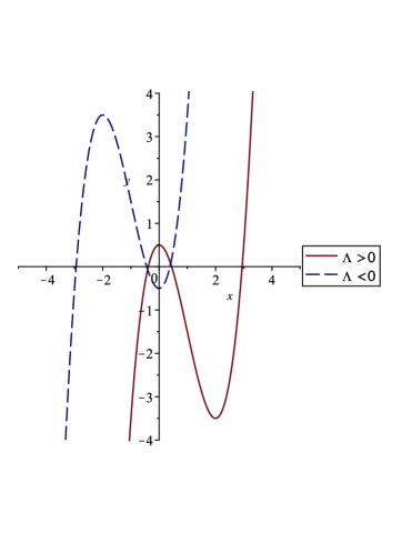
Figure 1: The graphs show the zeroes of the polynomial $F(x)$ with the positive discriminant, $\mathbf{Q}^{2}<\lambda^{2}$, corresponding to the solutions for horizon radius $x=v_{2}>0$ of the three-dimensional space $\Sigma_{k}$. When $\Lambda>0$ (continuous line), there are two solutions. When $\Lambda<0$ (dashed line), there is only one solution. The number of the solutions does not depend of the values of the parameters; the graphs are drawn for $\mathbf{Q}=1$ and $\Lambda=\pm 2$.

1. $\delta_{5}>0$. There are three different real roots because the cubic function in $v_{2}$ has a threefold intersection with the $v_{2}$-axis. This holds for

   $$\delta_{5}>0\quad\Rightarrow\quad Q^{2}<\frac{8k}{\varkappa\Lambda^{2}}\,,$$ (9.3)

   which in turn is possible only for spherical horizons ($k=1$), and when the charge (and the mass) of the extremal RN_Λ black hole are small. By simplifying the notation as $v_{2}=:x$, $\Lambda^{-1}=:\frac{\lambda}{2}$ and $\frac{\varkappa Q^{2}}{2}=:\mathbf{Q}^{2}$, we can analyze the curve $F(x)=x^{3}-\frac{3\lambda}{2}\,x^{2}+\frac{\lambda}{2}\,\mathbf{Q}^{2}$. The condition of positive discriminant means that $\mathbf{Q}^{2}<\lambda^{2}$. It holds that lim${}_{x\rightarrow\pm\infty}F(x)=\pm\infty$, whereas the extrema are at $0=F^{\prime}(x)=3x\left(x-\lambda\right)$, namely at the points $x=0$ and $x=\lambda$, for which $F(0)=\frac{\lambda}{2}\mathbf{Q}^{2}$ resp. $F(\lambda)=\frac{\lambda}{2}\left(\mathbf{Q}^{2}-\lambda^{2}\right)$. Since $F^{\prime\prime}(x)=3\left(2x-\lambda\right)$, it then holds that $F^{\prime\prime}(0)=-3\lambda$ and $F^{\prime\prime}(\lambda)=3\lambda$. Therefore, there is always one minimum and one maximum, depending on the sign of $\lambda$. When $\lambda>0$, both extrema are in the $x\geq 0$ half-plane, namely at $x=0$ and $x=\lambda$. Since $F^{\prime\prime}(0)=-3\lambda$, $x=0$ is the maximum which corresponds to $F_{\max}=\frac{\lambda}{2}\mathbf{Q}^{2}>0$; analogously, since $F^{\prime\prime}(\lambda)=3\lambda>0$, $x=\lambda$ is the minimum, corresponding to $F_{\min}=\frac{\lambda}{2}\left(\mathbf{Q}^{2}-\lambda^{2}\right)<0$. This shape of the cubic curve $F(x)$ is such that it intersects the $x$-axis exactly twice in the positive half-plane, and this implies that there are always, for any choice of parameters, exactly two positive real zeros (with the third real zero being always negative, and thence to be disregarded). Therefore, for $\lambda>0$, there are always two different solutions $v_{2}$, one in the interval $0<v_{2}<\frac{2}{\Lambda}$ (corresponding to $0<x<\lambda$) and another in the interval $v_{2}>\frac{2}{\Lambda}$ (corresponding to $x>\lambda$). When $\lambda<0$, both extrema are in the $x\leq 0$ half-plane, namely at $x=0$ and $x=\lambda$. Since $F^{\prime\prime}(0)=-3\lambda$, $x=0$ is the minimum, corresponding to $F_{\min}=\frac{\lambda}{2}\mathbf{Q}^{2}<0$, while, since $F^{\prime\prime}(\lambda)=3\lambda$, $x=\lambda$ is the maximum, corresponding to $F_{\max}=\frac{\lambda}{2}\left(\mathbf{Q}^{2}-\lambda^{2}\right)>0$. This shape of the cubic curve $F(x)$ is such that it intersects the $x$-axis exactly once in the positive half-plane, and this implies that there is always, for any choice of parameters, exactly one positive real zero (with the other two real zeros being always negative, and thus to be disregarded). Therefore, for $\lambda<0$, there is always exactly one solution $v_{2}>0$. The function $F(x)$ in the cases of positive and negative cosmological constant is shown in Fig. 1, where only its right half-plane zeros correspond to the physical solutions of the radius $v_{2}$.

2. $\delta_{5}=0$. There are two different real roots $v_{2}^{(1)}$ and $v_{2}^{(2)}$ in (9.1), because one of them is multiple ($v_{2}^{(2)}=v_{2}^{(3)}$) as the cubic function intersects only once the $v_{2}$-axis, and a second time it touches it. This means that the charge is fixed, and the positivity of $Q^{2}$ allows only for $k=1$,

   $$\delta_{5}=0\quad\Rightarrow\quad Q^{2}=\frac{8}{\varkappa\Lambda^{2}}\,,\quad k=1\,.$$ (9.4)

3. $\delta_{5}<0$. There is only one real root (the other two being complex), and thus

   $$\delta_{5}<0\quad\Rightarrow\quad Q^{2}>\frac{8k}{\varkappa\Lambda^{2}}\,.$$ (9.5)

   As we can see, this is possible for any kind of non-planar horizon (i.e., for $k=\pm 1$) : hyperbolic horizons can have arbitrary charge, whereas spherical horizons must have large charge (and large mass).

However, also in the cases 2 and 3 only positive values $v_{2}^{(i)}$ are physically meaningful, so only a subset of the solutions corresponding to (9.4) and (9.5) will give rise to a consistent radius of the three-dimensional transversal section $\Sigma_{k}$ of the extremal RN_Λ black hole. The above analysis shows that the number of real positive solutions for $v_{2}$ is always fixed for given parameters, whose precise value is not relevant for a qualitative analysis. Below, we list some explicit examples of the values of these parameters (for simplicity’s sake, we set $\varkappa=1$), corresponding to three broad classes (distinguished by labels A, B and C, as in (5.13)) :

$$1:\delta_{5}>0\quad\vskip 6.0pt plus 2.0pt minus 2.0pt$$ Class A

Class B

Class C —– —–

Class A

Class B

Class C —– —–

Class A —– —– (see below, also for )

Class B

Class C

The straight line means that no real positive solution exists for $v_{2}$. With the above reasoning, we have proved that there is no solution when $\delta_{5}\geq 0$ and $k=-1$. Now, we will show that there is no positive solution for $v_{2}$ when $\delta_{5}<0$ and $\Lambda>0$, for any kind of non-planar horizon (i.e., for $k=\pm 1$). We start by observing that $\delta_{5}<0$ implies $Y$ in (9.2) to be real, and thus $v_{2}^{(2,3)}$ are complex. Moreover, by setting $k=1$, the first of Eqs. (9.1) yields

$$v_{2}^{(1)}=1+\frac{Y}{2}+\frac{2}{Y}\,,$$ (9.6)

where, since $Y$ (9.2) depends on $\Lambda$ through the product $Q\Lambda$ and $\Lambda>0$, we have chosen $\Lambda=1$, obtaining

$$Y=\left(8-2Q^{2}+2Q\sqrt{Q^{2}-8}\right)^{1/3}<0\,,\qquad\text{ when }Q^{2}>8\,,$$ (9.7)

where we have assumed $Q>0$ without loss of generality. Therefore, for $v_{2}^{(1)}$ in (9.6) to be positive, it must hold that $\frac{Y}{2}+\frac{2}{Y}>-1$, which is impossible for $Y<0$. On the other hand, when $k=-1$, the first of Eqs. (9.1) yields

$$v_{2}^{(1)}=-1+\frac{Y}{2}+\frac{2}{Y}\,,$$ (9.8)

where, again, we have chosen $\Lambda=1$, obtaining

$$Y=\left(-8-2Q^{2}+2Q\sqrt{Q^{2}-8}\right)^{1/3}<0\,,\qquad\text{when }Q^{2}>8\,,$$ (9.9)

where again we have assumed $Q>0$ without loss of generality. Therefore, for $v_{2}^{(1)}$ in (9.8) to be positive, it must hold that $\frac{Y}{2}+\frac{2}{Y}>1$, which is impossible for $Y<0$. This means that there is no positive solution for $v_{2}$, q.e.d..

9.2 Entropy : with or without hair

Let us now study the $D=5$ extremal black hole near the critical point $Q_{c}$. The near-critical expansions of the extremal black hole entropies, in absence and presence of a non-trivial scalar hair (corresponding to the RN_Λ resp. the hairy black hole) read

$$\mathring{S} = S_{c}+2\pi\Omega_{3}e_{c}\,\epsilon+\mathring{S}_{2}\,\epsilon^{2}+\mathcal{O}(\epsilon^{3})\,,$$ (9.10)

$$S = S_{c}+2\pi\Omega_{3}e_{c}\,\epsilon+\mathring{S}_{2}\,\omega\epsilon^{2}+\mathcal{O}(\epsilon^{3})\,,$$ (9.11)

where the quadratic order $\mathring{S}_{2}$ of the entropy $\mathring{S}$ (i.e., with no scalar hair : $u=0$) is given by Eqs. (7.4) and (7.5) with $D=5$, yielding

$$\mathring{S}_{2}=\frac{k\pi\Omega_{3}}{6}\sqrt{\frac{k\Lambda\left(\varkappa m^{2}-1\right)}{2\varkappa m^{2}-3}}\left(\varkappa m^{2}-1\right)^{2}\left(4\varkappa m^{2}-3\right)\,.$$ (9.12)

On the other hand, by setting $D=5$ and plugging (8.3)–(8.5) into (8), the quadratic order $S_{2}$ of the entropy $S$ (i.e., with scalar hair : $u\neq 0$) can be computed to read

$$S_{2}=\frac{k\pi\Omega_{3}}{12\Lambda}\sqrt{\frac{k\Lambda(\varkappa m^{2}-1)}{2\varkappa m^{2}-3}}\frac{\left(\varkappa m^{2}-1\right)}{\left(\mathbf{c}_{0}-\mathbf{c}\right)}^{2}\left[\rule{0.0pt}{14.0pt}\varkappa m^{4}\left(2\varkappa m^{2}-3\right)-2\Lambda\mathbf{c}\left(4\varkappa m^{2}-3\right)\right]\,.$$ (9.13)

As resulting from (8.11), at the first order in $\epsilon$ there is no dependence of the RN_Λ extremal black hole entropy on the ‘effective interaction’ $\mathbf{c}$ (8.2). On the other hand, the dependence on $\mathbf{c}$ appears at the second order in $\epsilon$ in the expansion of the extremal hairy black hole entropy. Furthermore, $\mathbf{c}_{0}$ is given by (7.5) which, for $D=5$, becomes

$$\mathbf{c}_{0}=\frac{m^{2}}{6\Lambda}\,(2\varkappa m^{2}-3)(4\varkappa^{2}m^{4}-13\varkappa m^{2}+12)>0\,,$$ (9.14)

which is strictly positive as a consequence of the inequalities (5.12), as well as from the fact that $4y^{2}-13y+12>0$, $\forall y$.

The comparison of the quadratic terms of (9.10) and (9.11), namely of (9.12) and (9.13), allows one to define

$$\omega:=\frac{S_{2}}{\mathring{S}_{2}}=1+\frac{2m^{2}(\varkappa m^{2}-1)(2\varkappa m^{2}-3)^{3}}{3\Lambda(4\varkappa m^{2}-3)\left(\mathbf{c}-\mathbf{c}_{0}\right)}\,,$$ (9.15)

which is the unique source of dependence of (9.11) on $\mathbf{c}$, at the second order in $\epsilon$ included.

The factor $\omega$ plays the crucial role of determining which entropy is larger, and therefore it decides which state of the extremal black hole will be realised for given electric charge density $Q$, depending on the sign $\mathring{S}_{2}$ (9.12):

• when $\mathring{S}_{2}>0$, the hairy black hole has larger entropy than the RN_Λ black hole and thus a spontaneous scalarization takes place, when $\omega>1$;

• when $\mathring{S}_{2}<0$, the hairy black hole has larger entropy than the RN_Λ black hole and thus a spontaneous scalarization takes place, when $\omega<1$.

A detailed case study analysis yields that $\mathring{S}_{2}$ (9.12) is always positive, so the larger entropy solution always has $\omega>1$, except in the (example pertaining to the) class C above, in the interval of scalar masses $\varkappa m^{2}\in\left(\frac{3}{4},1\right)$ : in such a case, $\mathring{S}_{2}$ (9.12) becomes negative and the larger entropy solution has $\omega<1$. In all cases, regardless the sign of $k=\pm 1$, the spontaneous scalarization of the extremal black hole occurs if the ‘effective interaction’ $\mathbf{c}$ is positive and strong enough, namely if

$$\mathbf{c}>\mathbf{c}_{0}>0\,.$$ (9.16)

Apart from the sign of $\omega-1$, we should also ensure that the scalar hair $u$ is well defined, i.e., a real (positive) number; from the first of the near-critical expansions (8.1), this depends on the sign of the coefficient $A$, whose expression, by recalling (5.9), (5.10) and the first of Eqs. (8.3), reads for $D=5$ as follows :

$$A=\frac{2k\Lambda\left(\varkappa m^{2}-1\right)^{2}\sqrt{2km^{2}\left(\varkappa m^{2}-1\right)}}{3\left(\mathbf{c}_{0}-\mathbf{c}\right)}\,.$$ (9.17)

From (5.12), the critical coefficient $A$ is always real and, since (9.16) yields $\mathbf{c}_{0}-\mathbf{c}<0$, its sign coincides with the sign of $-k\Lambda$, as expressed by Eq. (8.6). Considering all the (examples pertaining to the) classes A, B and C discussed above, we obtain the following near-critical solutions for the scalar field $u$,

$$u_{\mathbf{A},\mathbf{C}}(Q) \simeq \sqrt{A(Q-Q_{c})}\,\mathcal{H}\left(Q_{c}-Q\right)\,,$$

$$u_{\mathbf{B}}(Q) \simeq \sqrt{A(Q-Q_{c})}\,\mathcal{H}\left(Q-Q_{c}\right)\,,$$ (9.18)

where $\mathcal{H}(Q)$ is the Heaviside step function which vanishes for negative arguments. Thus, it is worth remarking that the scalar field always condensates on only one side of the critical point $Q=Q_{c}$.

To summarize, for each of the (classes defined by the) boundary conditions determined by the pair $(\Lambda,k)$, there is a range of the scalar masses $m^{2}$, as given in (5.13), for which the spontaneous scalarization in $D=5$ spacetime dimensions takes place above or below the critical electric charge density $Q_{c}$, because the corresponding extremal hairy black hole becomes thermodynamically more stable than the electrically charged extremal RN_Λ black hole. In all cases, the process depends on the ‘effective coupling constant’ $\mathbf{c}$ defined by (8.2) : the value of $\mathbf{c}$ has to be larger than $\mathbf{c}_{0}$ given by (9.14) for the phase transition to occur, as expressed by the condition (9.16). Recalling that $\epsilon=Q-Q_{c}$ (cfr. the fifth Eq. of (6.1)), from the near-critical expansions (9.10)–(9.11) it is evident that the phase transition determined by the spontaneous scalarization of the electrically charged extremal RN_Λ black hole is characterized by the discontinuity of the response function $S^{\prime\prime}(Q)$,

$$\lim_{Q\to Q_{c}^{+}}S^{\prime\prime}(Q)\neq\lim_{Q\to Q_{c}^{-}}S^{\prime\prime}(Q),$$ (9.19)

thus implying that the phase transition that occurs at $Q=Q_{c}$ is a second order one.

9.3 Stueckelberg versus Higgs

We have observed that, near the critical point, only the effective coupling constant $\mathbf{c}$, defined by (8.2), matters. This feature does not hold away from criticality, because the Stueckelberg non-minimal interaction modifies the kinetic term as in the $\sigma$-model, while the Higgs interaction modifies only the potential. However, at the (unique) event horizon of the extremal black hole and near criticality, such two interacting terms do not play separate roles.

9.3.1 Symmetry enhancement at the critical point?

The (apriori unreasonable) effectiveness of $\mathbf{c}$ can be better appreciated by considering the scalar field effective potential, obtained as the total potential of the scalar field that includes electromagnetic and gravitational interaction [45],

$$V_{\mathrm{eff}}\left(\Psi\right):=V\left(\Psi\right)+\frac{1}{2}\,P\left(\Psi\right)\mathbf{A}^{2}=\frac{1}{2}\left(m^{2}+\mathbf{A}^{2}\right)\Psi^{2}+\frac{1}{4}\left(\dfrac{a}{2}\,\mathbf{A}^{2}+b\right)\Psi^{4}\,,$$ (9.20)

where

$$\mathbf{A}^{2}:=g^{\mu\nu}A_{\mu}A_{\nu}\,.$$ (9.21)

The equilibrium points for the scalar field are found from $V_{\mathrm{eff}}^{\prime}(\Psi)=0$, solved by

$$\Psi=0\,,\quad\text{and}\qquad\Psi_{0}^{2}=-\frac{\mathbf{A}^{2}+m^{2}}{\dfrac{a}{2}\,\mathbf{A}^{2}+b}\,,$$ (9.22)

respectively, corresponding to the local extrema of the potential,

$$V_{\mathrm{eff}}\left(0\right)=0\,,\quad\text{and}\qquad V_{\mathrm{eff}}\left(\Psi_{0}\right)=-\frac{1}{4}\,\frac{\left(\mathbf{A}^{2}+m^{2}\right)^{2}}{\dfrac{a}{2}\,\mathbf{A}^{2}+b}\,.$$ (9.23)

The effective mass

$$m_{\mathrm{eff}}^{2}\left(\Psi\right):=V_{\mathrm{eff}}^{\prime\prime 2}+\mathbf{A}^{2}+3\left(\dfrac{a}{2}\,\mathbf{A}^{2}+b\right)\Psi^{2}\,,$$ (9.24)

when non-vanishing, determines the unstable (maximum) or stable (minimum) nature of the critical points. It is an on-shell quantity and it clearly depends not only on the value of the scalar, but also on the value of the electromagnetic and gravitational fields through $\mathbf{A}^{2}$ (9.21), and therefore it involves the whole dynamics.

At the horizon $\mathbf{A}^{2}(r_{h})=-\frac{e^{2}}{v_{1}}$, and close to the critical point $\frac{e^{2}}{v_{1}}=m^{2}+\mathcal{O}(\epsilon)$, one obtains that $\mathbf{A}^{2}+m^{2}=\mathcal{O}(\epsilon)$ vanishes, and the effective coupling constant $\mathbf{c}$ (8.2) comes from the $\mathbf{A}^{2}$-interaction,

$$\dfrac{a}{2}\,\mathbf{A}^{2}+b=-\dfrac{m^{2}a-2b}{2}+\mathcal{O}(\epsilon)=:-\dfrac{\mathbf{c}}{2}+\mathcal{O}(\epsilon)\,.$$ (9.25)

Thus, the effective constant $\mathbf{c}$ arises naturally on the horizon and near criticality, i.e. when $Q\simeq Q_{c}$, and it is invariant under the exchange

$$am^{2}\leftrightarrow-2b\,.$$ (9.26)

This symmetry concerns all the horizon parameters up to linear order, as well as the black hole entropy up to quadratic order. However, the equations of motion in the near-horizon geometry are not invariant under (9.26). The fact that this property does not hold for general $Q$ (and thus away from $Q_{c}$) can be appreciated by continuing the near-$Q_{c}$ power-series expansion; by doing so, one would find that all horizon parameters, as well as the entropy, acquire terms which separately depend on $a$ and $b$, and which thus cannot be expressed only in terms of $\mathbf{c}$. This hints to a possible symmetry enhancement at $Q\simeq Q_{c}$ related to scale invariance and the answer, which can be obtained by analyzing near-horizon asymptotic isometries of the spacetime, surely deserves further investigation.

9.3.2 Effective mass and scalar condensation

On the other hand, to understand why the scalar field condensates and the scalarization takes place, we have to find its on-shell effective mass at the extremum points, which respectively reads

$$m_{\mathrm{eff}}^{2}(0)=m^{2}+\mathbf{A}^{2}\,,\qquad m_{\mathrm{eff}}^{2}\left(\Psi_{0}\right)=-2\left(\mathbf{A}^{2}+m^{2}\right)\,.$$ (9.27)

Since $m_{\mathrm{eff}}^{2}\left(0\right)$ and $m_{\mathrm{eff}}^{2}\left(\Psi_{0}\right)$ have opposite signs, only one of these two points is a (stable) minimum for a given set of parameters : it ultimately depends on the whole dynamics, because the equations of motion for $A_{\mu}(x)$ and $g_{\mu\nu}(x)$ have to be solved. Furthermore, the sign of $m_{\mathrm{eff}}^{2}$ itself also depends on the (squared) mass of the scalar field. Thus, the existence of another non-vanishing minimum $\Psi_{0}\neq 0$ depends on the full fledged dynamics of the electromagnetic, gravitational and scalar fields, as well as on the (choice of) values of coupling constants.

Since we are considering extremal black holes, the attractor mechanism [60] is at work, and it yields to a proper (i.e., stable) attractor value $u$ at the event horizon if and only if $u$ is a local minimum, i.e. if it has a positive effective mass, $m_{\mathrm{eff}}^{2}(u)>0$ (see e.g. [73]). In the framework under consideration, (9.27) implies in any $D\geq 4$ that

$$m_{\mathrm{eff}}^{2}(u)=-2\left(m^{2}-\frac{e^{2}}{v_{1}}\right)=-2m_{\mathrm{eff}}^{2}(0)\,,$$ (9.28)

and the result in turn depends on the solution for $e$ and $v_{1}$ obtained from other equations.

Eq. (9.28) yields that, if $u=0$ is a proper attractor ($m_{\mathrm{eff}}^{2}(0)>0$), then $u\neq 0$ is not a proper attractor, but rather a repeller, with $m_{\mathrm{eff}}^{2}(u)<0$, and the other way around: if $u\neq 0$ is a proper attractor, then $u=0$ is a repeller critical point :

• when $u=0$, a proper and unique attractor ($m_{\mathrm{eff}}^{2}(0)>0$ ), then Higgs potential $\approx$ Stueckelberg interaction, and the scalar hair $u\neq 0$ corresponds to a repeller critical point, with $m_{\mathrm{eff}}^{2}(u)<0$;

• when the scalar hair $u\neq 0$ corresponds to a proper (i.e. stable) attractor ($m_{\mathrm{eff}}^{2}(u)>0$), $u=0$ is a repeller critical point ($m_{\mathrm{eff}}^{2}(0)<0$) and the contribution of the Higgs and Stueckelberg interactions to $V_{\mathrm{eff}}$ can be interchanged by

  $$2b\leftrightarrow-a\,\frac{e^{2}}{v_{1}}\,,$$ (9.29)

  which follows from (9.26) and (9.28).

Clearly, without any interaction ($a=b=0$), it holds that $m_{\mathrm{eff}}^{2}=m^{2}\geq 0$, so $u=0$ is the only solution, and no phase transition takes place. On the other hand, the expansion of the effective mass (9.28) near the critical point $Q=Q_{c}$ yields

$$m_{\mathrm{eff}}^{2}(u)=-\frac{2e_{c}}{v_{1c}^{2}}\,\left(e_{c}\,B-2v_{1c}E\right)\left(Q-Q_{c}\right)+\mathcal{O}(\left(Q-Q_{c}\right)^{2})\,.$$ (9.30)

Using (8.4) and (8.5), this expression can be recast, in any dimension, in the following form :

$$m_{\mathrm{eff}}^{2}(u)=2\mathbf{c}A\left(Q_{c}-Q\right)+\mathcal{O}(\left(Q-Q_{c}\right)^{2})>0\,.$$ (9.31)

Thus, the effective mass of the scalar condensate is manifestly always positive on one side of the critical point, because (9.18) yields that $\mathrm{sgn}(Q-Q_{c})=\mathrm{sgn}(A)$ and $\mathbf{c}$ is positive (cfr. (9.16)). Crossing the critical point, the solution for $u$, as given by (9.18) for the various classes under consideration, vanishes and it yields $m_{\mathrm{eff}}^{2}(0)=0$, becoming the unique attractor point.

It is worth remarking here that, when $\Lambda<0$, it is known that the scalar equation in AdS_D spacetime admits a stable solution (under mechanical perturbations) for the scalar masses satisfying the Breitenlohner-Freedman bound [74, 75], $m_{\mathrm{eff}}^{2}\ell^{2}>-\frac{(D-1)^{2}}{4}$, where $\ell=\sqrt{\frac{(D-1)(D-2)}{2|\Lambda|}}$ is the AdS radius. Since in our case $m_{\mathrm{eff}}^{2}$ is positive, this bound is always satisfied. It does not mean, however, that the system is also thermodynamically stable. Indeed, the spontaneous scalarization could occur in the extremal cases when the particular conditions among the parameters are met, classified by intervals A, B or C. To prove that such thermodynamically unstable extremal black hole solutions exist in the whole space, it is necessary to solve the full fledged equations of motion.

Let us now discuss the above results within the classes A, B and C introduced in the previous treatment. We will consider the entropy density per horizon surface unit; for simplicity’s sake, we will set $\Omega_{3}=1$, $|\Lambda|=1$ and $\varkappa=1$. Also, the mass $m^{2}$ will be fixed, so that we can analyze the effect of interactions through the effective coupling $\mathbf{c}$, but the obtained results are valid generically within a given class.

Class A

Within this class, the extremal black hole without scalar hair is an electrically charged and asymptotically dS₅ Tangherlini black hole. The scalar field has mass $m^{2}=2$ and the ‘effective coupling’ is strong enough if $\mathbf{c}>\frac{2}{3}$, with respect to the value $\mathbf{c}_{0}=\frac{2}{3}$. Hence, the entropy density has the form

$$S(Q)=\left\{\begin{array}[]{lll}2\pi+2\pi\,(Q-Q_{c})+\dfrac{5\pi}{6}\,\left(Q-Q_{c}\right)^{2}+\mathcal{\cdots}\,,&Q\geq Q_{c},&\text{{\small Tangherlini~{}dS}}_{5}~{}\text{{\small BH};}\\ &&\\ 2\pi+2\pi\,(Q-Q_{c})+\dfrac{5\pi}{6}\dfrac{\left(\mathbf{c}-\frac{2}{5}\right)}{\left(\mathbf{c}-\frac{2}{3}\right)}\,\left(Q-Q_{c}\right)^{2}+\cdots\,,&Q\leq Q_{c},&\text{{\small sph.~{}hairy~{}dS}}_{5}~{}\text{{\small BH},}\end{array}\right.$$ (9.32)

and the order parameter (i.e., the value of the scalar field at the horizon) reads

$$u(Q)=\left\{\begin{array}[]{ll}0\,,&Q\geq Q_{c}\,,\vskip 6.0pt plus 2.0pt minus 2.0pt\\ \frac{2}{\sqrt{3}}\sqrt{\dfrac{Q_{c}-Q}{\mathbf{c}-\frac{2}{3}}}+\cdots\,,&Q\leq Q_{c}\,.\end{array}\right.$$ (9.33)

Thus, for large charges, i.e. for $Q\geq Q_{c}$, the extremal black hole is an asymptotically dS₅ Tangherlini black hole, with no scalar hair. Since $\dfrac{\mathbf{c}-\frac{2}{5}}{\mathbf{c}-\frac{2}{3}}>1$, as the electric charge density decreases to approach $Q_{c}$ from the right, the scalar field starts to condensate spontaneously on the horizon, because when $Q\leq Q_{c}$ the corresponding hairy extremal black hole has a higher entropy. As resulting from (9.32) (and as discussed above), the phase transition corresponding to the scalarization is of second order.

It is also instructive to show that, as we go farther from the critical point, the system begins to depend on both coupling constants $a$ and $b$ (occurring in (2.10)) separately, and not only on $\mathbf{c}$. For example, from the critical expansion (8.1) of the attractor horizon value $u$ of the scalar field, the sub-leading term reads

$$\sqrt{(K\epsilon)^{3}}=\sqrt{\frac{\epsilon^{3}}{A}}\frac{-33\mathbf{c}^{2}+12(2a-3)\mathbf{c}+4(2a+3)}{2\left(3\mathbf{c}-2\right)^{3}}\,.$$ (9.34)

In the above expression, the coupling $a$ appears as an independent parameter, but it does affect the value of the scalar (9.33) and the entropy (9.32) until the relevant order in $\epsilon$. However, as we depart farther from the horizon, the scalar field is well defined only if (9.34) is positive, which is possible (with $\mathbf{c}>\frac{2}{3}$ and $A\epsilon>0$) only when the polynomial in the numerator is positive. Because the numerator geometrically presents a mostly negative hyperbola in $\mathbf{c}$, the conditions in $a$ have to ensure an existence of a positive section of the hyperbola, that is,

$$\frac{2}{3}<\mathbf{c}\leq\frac{2}{11}\left(2a-3+\frac{1}{3}\sqrt{a^{2}-\frac{7a}{6}+5}\right)\,,$$ (9.35)

where one root is smaller than $\frac{2}{3}$. The right bound is real for any $a$ and it is bigger than $\frac{2}{3}$ when $a>\frac{9}{10}$. Thus, there are infinitely many possibilities for the coupling constants $a$ and $\mathbf{c}$ leading to the scalarization. Interestingly, neither too strong nor too weak coupling $\mathbf{c}$ will produce a scalarization. This situation (existence of the solution) is generic in all cases A, B or C, and we will not analyze it in other cases, as it does not influence the physics in the vicinity of the critical point.

Class B

Within this class, the extremal black hole without scalar hair is an electrically charged and asymptotically AdS₅ Tangherlini black hole. This scalar field has mass $m^{2}=\frac{6}{5}$, the strength of the interaction is measured with respect to $\mathbf{c}_{0}=2\left(\frac{3}{5}\right)^{4}=\frac{162}{625}$, and the effective coupling is $\mathbf{c}>\frac{162}{625}\simeq 0,29$. Hence, the entropy density has the form

$$S(Q)=\left\{\begin{array}[]{lll}6\sqrt{3}\pi+\dfrac{6\pi}{5}\,\left(Q-Q_{c}\right)+\dfrac{\sqrt{3}\pi}{250}\,\left(Q-Q_{c}\right)^{2}+\mathcal{\cdots}\,,&Q\leq Q_{c},&\text{Tangherlini~{}AdS}_{5}~{}\text{BH;}\\ &&\\ 6\sqrt{3}\pi+\dfrac{6\pi}{5}\,\left(Q-Q_{c}\right)+\dfrac{\sqrt{3}\pi}{250}\dfrac{\left(\mathbf{c}-\frac{6}{25}\right)}{\left(\mathbf{c}-\frac{162}{625}\right)}\,\left(Q-Q_{c}\right)^{2}+\mathcal{\cdots}\,,&Q\geq Q_{c},&\text{sph.~{}hairy~{}AdS}_{5}~{}\text{BH,}\end{array}\right.$$ (9.36)

and the order parameter reads

$$u(Q)=\left\{\begin{array}[]{ll}0\,,&Q\leq Q_{c}\,,\vskip 6.0pt plus 2.0pt minus 2.0pt\\ \frac{2}{5\sqrt{5}\sqrt[4]{3}}\sqrt{\dfrac{Q-Q_{c}}{\mathbf{c}-\frac{162}{625}}}+\cdots\,,&Q\geq Q_{c}.\end{array}\right.$$ (9.37)

Thus, for small charges, i.e. for $Q\leq Q_{c}$, the extremal black hole is an asymptotically AdS₅ Tangherlini black hole, with no scalar hair. Since $\dfrac{\mathbf{c}-\frac{6}{25}}{\mathbf{c}-\frac{162}{625}}>1$, as the electric charge density decreases to approach $Q_{c}$ from the left, the scalar field starts to condensate on the horizon, because when $Q\geq Q_{c}$ the corresponding hairy extremal black hole has a higher entropy. Again, as resulting from (9.36), the phase transition corresponding to the scalarization is of second order.

Class C (light scalar)

Within this class, the extremal black hole without scalar hair is the analogue of an electrically charged and asymptotically AdS₅ Tangherlini black hole, but with hyperbolic horizon ($k=-1$); let us denote it with “hypTangh.”. Consider a ‘light’ scalar field with mass $m^{2}=\frac{1}{2}$, with the strength of the effective interaction measured with respect to $\mathbf{c}_{0}=\frac{13}{12}$, and given by $\mathbf{c}>\frac{13}{12}$. Hence, the entropy density has the form

$$S(Q)=\left\{\begin{array}[]{lll}\sqrt{2}\pi+16\pi\left(Q-Q_{c}\right)+\dfrac{\pi}{48}\,\left(Q-Q_{c}\right)^{2}+\mathcal{\cdots}\,,&Q\geq Q_{c},&\text{hypTangh.~{}AdS }_{5}~{}\text{BH;}\\ &&\\ \sqrt{2}\pi+16\pi\left(Q-Q_{c}\right)+\dfrac{\pi}{48}\dfrac{\left(\mathbf{c}+\frac{1}{4}\right)}{\left(\mathbf{c}-\frac{13}{12}\right)}\,\left(Q-Q_{c}\right)^{2}+\mathcal{\cdots}\,,&Q\leq Q_{c},&\text{hyp.~{}hairy~{}AdS}_{5}~{}\text{BH,}\end{array}\right.$$ (9.38)

and the order parameter is

$$u(Q)=\left\{\begin{array}[]{ll}0\,,&Q\geq Q_{c}\,,\vskip 6.0pt plus 2.0pt minus 2.0pt\\ \frac{\sqrt[4]{2}}{2\sqrt{3}}\sqrt{\dfrac{Q_{c}-Q}{\mathbf{c}-\frac{13}{12}}}+\cdots\,,&Q\leq Q_{c}\,.\end{array}\right.$$ (9.39)

For large charges $Q\geq Q_{c}$, the extremal black hole is an asymptotically AdS₅ hyperbolic Tangherlini black hole, with no scalar hair. Because $\dfrac{\mathbf{c}+\frac{1}{4}}{\mathbf{c}-\frac{13}{12}}>1$, as the electric charge density decreases to approach $Q_{c}$ from the right, the scalar field condensates on the horizon since, when $Q\leq Q_{c}$, the corresponding hairy extremal black hole has a higher entropy. As in the other cases, the phase transition (9.38) corresponding to the scalarization is of second order.

Class C (heavy scalar)

Within the same class, we can consider a ‘heavy’ scalar field with mass $m^{2}=\frac{4}{5}$, with the strength of the effective interaction compared to $\mathbf{c}_{0}=\frac{91}{3}\left(\frac{2}{5}\right)^{4}=\frac{1,456}{1,875}$ and given by $\mathbf{c}>\frac{1,456}{1,875}$. Hence, the entropy density has the form

$$S(Q) = \left\{\begin{array}[]{lll}S_{01}(Q)-\dfrac{\sqrt{7}\pi}{5,250}\,\left(Q-Q_{c}\right)^{2}+\mathcal{\cdots}\,,&Q\geq Q_{c},&\text{hypTangh.~{}AdS}_{5}~{}\text{BH;}\\ &&\\ S_{01}(Q)-\dfrac{\sqrt{7}\pi}{5,250}\dfrac{\left(\mathbf{c}-\frac{4,200}{1,875}\right)}{\left(\mathbf{c}-\frac{1,456}{1,875}\right)}\,\left(Q-Q_{c}\right)^{2}+\mathcal{\cdots}\,,&Q\leq Q_{c}&\text{hyp.~{}hairy~{}AdS}_{5}~{}\text{BH,}\end{array}\right.$$ (9.43)

where $S_{01}(Q):=14\sqrt{7}\pi+\dfrac{2\sqrt{14}\pi}{5}\,\left(Q-Q_{c}\right)$ and its derivatives are continuous in the limit $Q\to Q_{c}$, and the order parameter is

$$u(Q)=\left\{\begin{array}[]{ll}0\,,&Q\geq Q_{c}\,,\\ \frac{2\sqrt[4]{2}}{5\sqrt{5}\sqrt{3}}\sqrt{\dfrac{Q_{c}-Q}{\mathbf{c}-\frac{1,456}{1,875}}}+\mathcal{\cdots}\,,&Q\leq Q_{c}\,,\vskip 6.0pt plus 2.0pt minus 2.0pt\end{array}\right.$$ (9.45)

Differently from all other classes treated above, in the ‘heavy scalar’ regime of the class C the second order term in the near-critical expansion of the extremal black hole entropy becomes negative, and thus a separate analysis is deserved.

For large charges, i.e. for $Q\geq Q_{c}$, the extremal black hole is an asymptotically AdS₅ hyperbolic Tangherlini black hole. Since $\dfrac{\mathbf{c}-\frac{4,200}{1,875}}{\mathbf{c}-\frac{1,456}{1,875}}<1$ (and $\lim\limits_{\mathbf{c}\rightarrow\infty}\dfrac{\mathbf{c}-\frac{4,200}{1,875}}{\mathbf{c}-\frac{1,456}{1,875}}=1^{-}$), as the electric charge density decreases to approach $Q_{c}$ from the right, the scalar field condensates on the horizon, because when $Q\leq Q_{c}$ the corresponding hairy extremal black hole has a higher entropy. From (LABEL:4-entropy), we can conclude that the phase transition corresponding to the scalarization is of second order.

10 Conclusions

We discuss thermodynamics of static, electrically charged extremal black holes in Einstein-Maxwell gravity coupled to a complex scalar field in $D$ dimensions, in presence of an arbitrary cosmological constant $\Lambda$. A non-minimal coupling of the scalar field is described by the non-linear Stueckelberg interaction and the Higgs potential, characterized by the coupling constants $a$ and $b$, respectively. The former modifies the kinetic term of the scalar field whereas the latter modifies the potential. When $a,b=0$, the coupling becomes minimal.

The relevant thermodynamic quantity of the extremal black holes is the entropy. We compute it using the entropy function formalism and analyse its global maxima describing stable states. We show that there is always a critical point, with the electric charge density $Q_{c}$, where the scalar field spontaneously condensates, leading to a thermodynamic instability of the Reissner-Nordström black hole. For a given background with $\Lambda\neq 0$ and the non-planar black hole horizon $k\neq 0$, we find three regions in the space of the solutions, called A, B and C, determined by the positive intervals of the scalar mass, $\varkappa m^{2}\neq 1,\frac{D-2}{D-3}$. In these sectors, the hairy extremal black hole is thermodynamically more stable than the electrically charged extremal Reissner-Nordström-(A)dS one, when the effective interaction is strong enough, $\mathbf{c}>\mathbf{c}_{0}$. We determine the critical exponents in the vicinity of the critical point. In particular, the order parameter has critical exponent $1/2$, the same as in the Landau-Ginsburg theory. In the Ehrenfest-like classification based on the behavior of the entropy, this phase transition is of second order, because the response function $S^{\prime\prime}(Q)$ has a discontinuity in $Q_{c}$. Out of the regions A, B and C, the extremal black hole is thermodynamically stable.

The effective coupling constant $\mathbf{c}=m^{2}a-2b$ appears due to the attractor mechanism of the extremal black holes, yielding a proper attractor value of the scalar field at the event horizon, $u$, for a positive effective mass, $m_{\mathrm{eff}}^{2}(u)=2A\mathbf{c}\left(Q_{c}-Q\right)>0$. Since $m_{\mathrm{eff}}^{2}(u)$ and $m_{\mathrm{eff}}^{2}(0)$ have opposite signs, when $u=0$ is a proper attractor, then $u\neq 0$ is a repeller, and vice versa. Away from criticality ($Q-Q_{c}$ is not small), both $a$ and $b$ play important roles, governed by the field equations, such that the Stueckelberg interaction modifies the kinetic term as in the $\sigma$-model, while the Higgs interaction modifies only the potential.

We work out five-dimensional case in detail. A typical process of scalarization goes as follows (on the example of the extremal black hole belonging to the class A): the strongly coupled ($\mathbf{c}>\mathbf{c}_{0}$) Tangherlini dS₅ extremal black hole, electrically charged with $Q>Q_{c}$, has vanishing scalar field. When we slowly decrease the charge so that the black hole remains extremal, after the critical point ($Q<Q_{c}$), the scalar field will start to condensate on the horizon, and forming a hairy black hole, which has larger entropy. This system describes a phase transition of second order. Similar situation occurs in cases B and C.

There are still many open questions related to spontaneous scalarization of extremal black holes. One of the most important ones is to find an explicit solution of the Einstein-Maxwell equations for a given boundary conditions, in one of the sectors A, B or C, which shows a phase transition. To this end, one should choose a good radial coordinate to be able to impose correct boundary conditions for extremal black holes, by introducing a warp factor and the extremality parameter, $\xi$, which is a measure of deviation of two different horizons $r_{+}>r_{-}$ from their extremal value $r_{h}$, that is, $r_{\pm}=r_{h}\pm\xi$. For the scalar to be regular, one needs the physical distance $\mathrm{d}\rho^{2}=\mathrm{e}^{-2U}\mathrm{d}r^{2}$ and $\Psi(\rho_{h})$ to be finite. Note that our radial coordinate appearing in AdS₂ is the distance from the horizon (thus located at $r=0$).

Another important step is embedding this model in supergravity and studying similar instabilities using particular forms of $V(\Psi)$ and $P(\Psi)$ coming from the gauged supergravity. In particular, it would be interesting to make $\sigma(x)$ a dynamic field within the $\sigma$-model, and study the exponential potential between the scalar field and the electrodynamics, as typically occurs in supergravity. Concerning the embedding in $D=5$ supergravity, since the model discussed here contains one Maxwell field and one complex scalar field, it cannot be regarded as the (purely) bosonic sector of any $\mathcal{N}\geq 2$ gauged supergravity. Still, it might be embedded in gauged supergravity with suitable truncation of the bosonic sector (namely, of the scalar and vector fields). If this were possible, it would then be interesting to see whether the relation between the $Q$, $\Lambda$ and $k$ is related to the BPS states. We leave the investigation of these issues to future work.

We also leave for further study an analysis of asymptotic symmetries near the horizon in the vicinity of the critical point, looking for the symmetry enhancement related to the scale invariance. We expect that only the effective constant $\mathbf{c}$ will play a relevant role in this approximation.

References

- [1] W. Israel, Event horizons in static vacuum space-times, Phys. Rev. 164, 1776–1779 (1967).
- [2] B. Carter, Axisymmetric black hole has only two degrees of freedom, Phys. Rev. Lett. 26, 331–333 (1971).
- [3] R. Ruffini, J.A. Wheeler, Introducing the black hole, Phys. Today 24(1), 30 (1971).
- [4] V. Cardoso, L. Gualtieri, Testing the black hole ‘no-hair’ hypothesis, Class. Quant. Grav. 33, no.17, 174001 (2016), arXiv:1607.03133 [gr-qc].
- [5] T. Damour, G. Esposito-Farese, Nonperturbative strong field effects in tensor–scalar theories of gravitation, Phys. Rev. Lett. 70, 2220–2223 (1993).
- [6] I.Z. Stefanov, S.S. Yazadjiev, M.D. Todorov, Phases of 4D scalar-tensor black holes coupled to Born–Infeld nonlinear electrodynamics, Mod. Phys. Lett. A23, 2915–2931 (2008), arXiv:0708.4141 [gr-qc].
- [7] D.D. Doneva, S.S. Yazadjiev, K.D. Kokkotas, I.Z. Stefanov, Quasi-normal modes, bifurcations and non-uniqueness of charged scalar-tensor black holes, Phys. Rev. D82, 064030 (2010), arXiv:1007.1767 [gr-qc].
- [8] V. Cardoso, I.P. Carucci, P. Pani, T.P. Sotiriou, Matter around Kerr black holes in scalar-tensor theories: scalarization and superradiant instability, Phys. Rev. D88, 044056 (2013), arXiv:1305.6936 [gr-qc].
- [9] V. Cardoso, I.P. Carucci, P. Pani, T.P. Sotiriou, Black holes with surrounding matter in scalar-tensor theories, Phys. Rev. Lett. 111, 111101 (2013), arXiv:1308.6587 [gr-qc].
- [10] M.S. Volkov, D.V. Galtsov, NonAbelian Einstein Yang–Mills black holes, JETP Lett. 50, 346–350 (1989).
- [11] P. Bizon, Colored black holes, Phys. Rev. Lett. 64, 2844–2847 (1990).
- [12] B.R. Greene, S.D. Mathur, C.M. O’Neill, Eluding the no hair conjecture: black holes in spontaneously broken gauge theories, Phys. Rev. D47, 2242–2259 (1993), hep-th/9211007.
- [13] H. Luckock, I. Moss, Black holes have skyrmion hair, Phys. Lett. B176, 341–345 (1986).
- [14] S. Droz, M. Heusler, N. Straumann, New black hole solutions with hair, Phys. Lett. B268, 371–376 (1991).
- [15] P. Kanti, N.E. Mavromatos, J. Rizos, K. Tamvakis, E. Winstanley, Dilatonic black holes in higher curvature string gravity, Phys. Rev. D54, 5049–5058 (1996), hep-th/9511071.
- [16] B. Kleihaus, J. Kunz and S. Yazadjiev, Scalarized Hairy Black Holes, Phys. Lett. B744 (2015), 406-412, arXiv:1503.01672 [gr-qc].
- [17] C.A.R. Herdeiro, E. Radu, Asymptotically flat black holes with scalar hair: a review, Int. J. Mod. Phys. D24(09), 1542014 (2015), arXiv:1504.08209 [gr-qc].
- [18] J. D. Bekenstein, Exact solutions of Einstein conformal scalar equations, Annals Phys. 82 (1974), 535-547.
- [19] N. M. Bocharova, K. A. Bronnikov, V. N. Melnikov, Instability of black holes with scalar charge (in Russian), Vestn. Mosk. Univ. Fiz. Astron. 6 (1970) 706.
- [20] A. Dima, E. Barausse, N. Franchini and T. P. Sotiriou, Spin-induced black hole spontaneous scalarization, Phys. Rev. Lett. 125 (2020) no.23, 231101, arXiv:2006.03095 [gr-qc].
- [21] C. A. R. Herdeiro, E. Radu, Static Einstein-Maxwell black holes with no spatial isometries in AdS space, Phys. Rev. Lett. 117 (2016) 221102, arXiv:1606.02302 [gr-qc].
- [22] C. A. R. Herdeiro, E. Radu, N. Sanchis-Gual, J. A. Font, Spontaneous scalarization of charged black holes, Phys. Rev. Lett. 121 (2018) 101102, arXiv:1806.05190 [gr-qc].
- [23] D. D. Doneva, S. S. Yazadjiev, New Gauss-Bonnet Black Holes with Curvature-Induced Scalarization in Extended Scalar-Tensor Theories, Phys. Rev. Lett. 120 (2018) no.13, 131103, arXiv:1711.01187 [gr-qc].
- [24] H. O. Silva, J. Sakstein, L. Gualtieri, T. P. Sotiriou, E. Berti, Spontaneous scalarization of black holes and compact stars from a Gauss-Bonnet coupling, Phys. Rev. Lett. 120 (2018) no.13, 131104, arXiv:1711.02080 [gr-qc].
- [25] G. Antoniou, A. Bakopoulos, P. Kanti, Evasion of no-hair theorems and novel black-hole solutions in Gauss–Bonnet theories, Phys. Rev. Lett. 120(13), 131102 (2018), arXiv:1711.03390 [hep-th].
- [26] D. D. Doneva, S. Kiorpelidi, P. G. Nedkova, E. Papantonopoulos, S. S. Yazadjiev, Charged Gauss-Bonnet black holes with curvature induced scalarization in the extended scalar-tensor theories, Phys. Rev. D98 (2018) no.10, 104056, arXiv:1809.00844 [gr-qc].
- [27] P.V.P. Cunha, C.A.R. Herdeiro, E. Radu, Spontaneously scalarized Kerr black holes in extended scalar-tensor-Gauss–Bonnet gravity, Phys. Rev. Lett. 123(1), 011101 (2019), arXiv:1904.09997 [gr-qc].
- [28] H. O. Silva, C. F. B. Macedo, T. P. Sotiriou, L. Gualtieri, J. Sakstein, E. Berti, Stability of scalarized black hole solutions in scalar-Gauss-Bonnet gravity, Phys. Rev. D99 (2019) no.6, 064011, arXiv:1812.05590 [gr-qc].
- [29] C.A.R. Herdeiro, E. Radu, H.O. Silva, T.P. Sotiriou, N. Yunes, Spin-induced scalarized black holes, Phys. Rev. Lett. 126(1), 011103 (2021), arXiv:2009.03904 [gr-qc].
- [30] E. Berti, L.G. Collodel, B. Kleihaus, J. Kunz, Spin-induced black-hole scalarization in Einstein-scalar-Gauss–Bonnet theory, Phys. Rev. Lett. 126(1), 011104 (2021), arXiv:2009.03905 [gr-qc].
- [31] Y. Brihaye, B. Hartmann, N. P. Aprile, J. Urrestilla, Scalarization of asymptotically anti de Sitter black holes with applications to holographic phase transitions, Phys. Rev. D101 (2020) no.12, 124016, arXiv:1911.01950 [gr-qc].
- [32] D. Astefanesei, C. Herdeiro, J. Oliveira, E. Radu, Higher dimensional black hole scalarization, JHEP 09 (2020) 186, arXiv:2007.04153 [gr-qc].
- [33] S. Hod, Onset of spontaneous scalarization in spinning Gauss-Bonnet black holes, Phys. Rev. D 102 (2020) no.8, 084060, arXiv:2006.09399 [gr-qc].
- [34] R. A. Konoplya, A. Zhidenko, Analytical representation for metrics of scalarized Einstein-Maxwell black holes and their shadows, Phys. Rev. D100 (2019) no.4, 044015, arXiv:1907.05551 [gr-qc].
- [35] S. Hod, Spontaneous scalarization of charged Reissner-Nordström black holes: Analytic treatment along the existence line, Phys. Lett. B798 (2019), 135025, arXiv:2002.01948 [gr-qc].
- [36] P.G.S. Fernandes, C.A.R. Herdeiro, A.M. Pombo, E. Radu, N. Sanchis-Gual, Spontaneous scalarisation of charged black holes: coupling dependence and dynamical features, Class. Quantum Gravity 36(13), 134002 (2019). [Erratum: Class. Quantum Gravity 37, 049501 (2020)], arXiv:1902.05079 [gr-qc].
- [37] J.L. Blázquez-Salcedo, C.A.R. Herdeiro, J. Kunz, A.M. Pombo, E. Radu, Einstein–Maxwell-scalar black holes: the hot, the cold and the bald, Phys. Lett. B806, 135493 (2020), arXiv: 2002.00963 [gr-qc].
- [38] D. Astefanesei, C. Herdeiro, A. Pombo, E. Radu, Einstein–Maxwell-scalar black holes: classes of solutions, dyons and extremality, JHEP 10, 078 (2019), arXiv: 1905.08304 [hep-th].
- [39] P.G.S. Fernandes, C.A.R. Herdeiro, A.M. Pombo, E. Radu, Charged black holes with axionic-type couplings: classes of solutions and dynamical scalarization, Phys. Rev. D100(8), 084045 (2019), arXiv:1908.00037 [gr-qc].
- [40] F. M. Ramazanoğlu, F. Pretorius, Spontaneous Scalarization with Massive Fields, Phys. Rev. D93 (2016) no.6, 064005, arXiv:1601.07475 [gr-qc].
- [41] C. F. B. Macedo, J. Sakstein, E. Berti, L. Gualtieri, H. O. Silva, T. P. Sotiriou, Self-interactions and Spontaneous Black Hole Scalarization, Phys. Rev. D99 (2019) no.10, 104041, arXiv:1903.06784 [gr-qc].
- [42] D. C. Zou, Y. S. Myung, Scalarized charged black holes with scalar mass term, Phys. Rev. D100 (2019) no.12, 124055, arXiv:1909.11859 [gr-qc].
- [43] P. G. S. Fernandes, Einstein-Maxwell-scalar black holes with massive and self-interacting scalar hair, Phys. Dark Univ. 30 (2020) 100716, arXiv:2003.01045 [gr-qc].
- [44] Y. Brihaye, C. Herdeiro, E. Radu, Black hole spontaneous scalarisation with a positive cosmological constant, Phys. Lett. B802, 135269 (2020), arXiv: 1910.05286 [gr-qc].
- [45] S. S. Gubser, Breaking an Abelian gauge symmetry near a black hole horizon, Phys. Rev. D78, 065034 (2008), arXiv:0801.2977 [hep-th].
- [46] S. A. Hartnoll, C. P. Herzog, G. T. Horowitz, Building a Holographic Superconductor, Phys. Rev. Lett. 101, 031601 (2008), arXiv:0803.3295 [hep-th].
- [47] S. A. Hartnoll, C. P. Herzog, G. T. Horowitz, Holographic Superconductors, JHEP 0812 (2008) 015, arXiv:0810.1563 [hep-th].
- [48] T. Nishioka, S. Ryu and T. Takayanagi, Holographic Superconductor/Insulator Transition at Zero Temperature, JHEP 03 (2010), 131 arXiv:0911.0962 [hep-th].
- [49] A. Marrani, O. Miskovic, P. Q. Leon, Extremal Black Holes, Stueckelberg Scalars and Phase Transitions, JHEP 02 (2018), 080, arXiv:1712.01425 [hep-th].
- [50] S. Franco, A. Garcia-Garcia, D. Rodriguez-Gomez, A General class of holographic superconductors, JHEP 1004 (2004) 092, arXiv:0906.1214 [hep-th].
- [51] Y. S. Myung, D. C. Zou, Instability of Reissner-Nordström black hole in Einstein-Maxwell-scalar theory, Eur. Phys. J. C 79 (2019) no.3, 273, arXiv:1808.02609 [gr-qc].
- [52] R. Gregory, R. Laflamme, Black strings and p-branes are unstable, Phys. Rev. Lett. 70 (1993), 2837-2840, hep-th/9301052.
- [53] Y. Brihaye, B. Hartmann, Spontaneous scalarization of charged black holes at the approach to extremality, Phys. Lett. B792 (2019), 244-250, arXiv:1902.05760 [gr-qc].
- [54] A. Sen, Black hole entropy function and the attractor mechanism in higher derivative gravity, JHEP 0509 (2005) 038, hep-th/0506177.
- [55] A. Sen, Entropy function for heterotic black holes, JHEP 0603 (2006) 008, hep-th/0508042.
- [56] E. Cremmer, J. Scherk, S. Ferrara, SU(4) Invariant Supergravity Theory, Phys. Lett. B 74 (1978) 61.
- [57] P. Fré, A. S. Sorin, M. Trigiante, Integrability of Supergravity Black Holes and New Tensor Classifiers of Regular and Nilpotent Orbits, JHEP 04 (2012) 015, arXiv:1103.0848 [hep-th].
- [58] E. C. G. Stueckelberg, Interaction forces in electrodynamics and in the field theory of nuclear forces, Helv. Phys. Acta 11 (1938) 299.
- [59] S. Ferrara, K. Hayakawa, A. Marrani, Lectures on Attractors and Black Holes, Fortsch. Phys. 56 (2008) 993, arXiv:0805.2498 [hep-th].
- [60] S. Ferrara, R. Kallosh, A. Strominger, extremal black holes, Phys. Rev. D52 (1995) 5412, hep-th/9508072. A. Strominger, Macroscopic Entropy of Extremal Black Holes, Phys. Lett. B383 (1996) 39, hep-th/9602111. S. Ferrara, R. Kallosh, Supersymmetry and Attractors, Phys. Rev. D54 (1996) 1514, hep-th/9602136. S. Ferrara, R. Kallosh, Universality of Supersymmetric Attractors, Phys. Rev. D54 (1996) 1525, hep-th/9603090.
- [61] G. T. Horowitz and M. M. Roberts, Zero Temperature Limit of Holographic Superconductors, JHEP 11 (2009) 015, arXiv:0908.3677 [hep-th].
- [62] M. Astorino, Magnetised Kerr/CFT correspondence, Phys. Lett. B 751 (2015) 96, arXiv:1508.01583 [hep-th].
- [63] J. Bičák and F. Hejda, Near-horizon description of extremal magnetized stationary black holes and Meissner effect, Phys. Rev. D 92 (2015) 104006, arXiv:1510.01911 [gr-qc].
- [64] M. Astorino, CFT Duals for Accelerating Black Holes, Phys. Lett. B 760 (2016) 393, arXiv:1605.06131 [hep-th].
- [65] G. T. Horowitz and B. Way, Complete Phase Diagrams for a Holographic Superconductor/Insulator System, JHEP 11 (2010) 011, arXiv:1007.3714 [hep-th].
- [66] A. Sen, Black Hole Entropy Function, Attractors and precision counting of microstates, Gen. Rel. Grav. 40 (2008) 2249, arXiv:0708.1270 [hep-th].
- [67] A. Gallerati, Constructing black hole solutions in supergravity theories, Int. J. Mod. Phys. A 34 (2020) 1930017, arXiv:1905.04104 [hep-th].
- [68] K. Saraikin, C. Vafa, Non-supersymmetric black holes and topological strings, Class. Quant. Grav. 25 (2008) 095007, hep-th/0703214.
- [69] G. W. Moore, Arithmetic and attractors, hep-th/9807087.
- [70] A. Giryavets, New attractors and area codes, JHEP 0603 (2006) 020, hep-th/0511215.
- [71] F. R. Tangherlini, Schwarzschild field in dimensions and the dimensionality of space problem, Nuovo Cimento 27, 636 (1963).
- [72] R. C. Myers, M. J. Perry, Black Holes in Higher Dimensional Space-Times, Ann. Phys. 172, 304 (1986).
- [73] K. Goldstein, N. Iizuka, R. P. Jena, S. P. Trivedi, Non-supersymmetric attractors, Phys. Rev. D72 (2005) 124021, hep-th/0507096.
- [74] P. Breitenlohner, D. Z. Freedman, Stability in gauged extended supergravity, Annals Phys. 144 (1982) 249.
- [75] P. Breitenlohner, D. Z. Freedman, Positive energy in anti-de Sitter backgrounds and gauged extended supergravity, Phys. Lett. B115 (1982) 197.