Benchmarking Deep AUROC Optimization:
Loss Functions and Algorithmic Choices

Abstract

The area under the ROC curve (AUROC) has been vigorously applied for imbalanced classification and moreover combined with deep learning techniques. However, there is no existing work that provides sound information for peers to choose appropriate deep AUROC maximization techniques. In this work, we fill this gap from three aspects. (i) We benchmark a variety of loss functions with different algorithmic choices for deep AUROC optimization problem. We study the loss functions in two categories: pairwise loss and composite loss, which includes a total of 10 loss functions. Interestingly, we find composite loss, as an innovative loss function class, shows more competitive performance than pairwise loss from both training convergence and testing generalization perspectives. Nevertheless, data with more corrupted labels favors a pairwise symmetric loss. (ii) Moreover, we benchmark and highlight the essential algorithmic choices such as positive sampling rate, regularization, normalization/activation, and optimizers. Key findings include: higher positive sampling rate is likely to be beneficial for deep AUROC maximization; different datasets favors different weights of regularizations; appropriate normalization techniques, such as sigmoid and $\ell_{2}$ score normalization, could improve model performance. (iii) For optimization aspect, we benchmark SGD-type, Momentum-type, and Adam-type optimizers for both pairwise and composite loss. Our findings show that although Adam-type method is more competitive from training perspective, but it does not outperform others from testing perspective.

Keywords: AUROC optimization, deep learning, benchmark

1 Introduction

It is widely accepted that the area under the ROC curve (AUROC) (Hanley and McNeil, 1982) is a better metric than accuracy for classification problems on imbalanced datasets because the majority class could be dominating in the calculation of the accuracy metric and the surrogate loss function as well for model training process. On the other hand, AUROC evaluates how well a model classifies positive samples given threshold fixed by every negative sample. Alternatively, AUROC could also be interpreted as the probability that a random positive sample enjoys a larger predicted value than a random negative sample. AUROC metric has been applied in a variety of areas, such as, medical imaging diagnosis, molecular property prediction, natural hazards, meteorology (Irvin et al., 2019; Wu et al., 2018; Peres and Cancelliere, 2014; Murphy, 1996); and potentially any imbalanced datasets. Moreover, deep learning has been achieving many successes since last decade in many areas, such as, computer vision, natural language processing, molecular property prediction (Krizhevsky et al., 2012; Vaswani et al., 2017; Wu et al., 2018). Given that deep learning could handle more complicated tasks than traditional machine learning, it is unavoidable to consider optimizing AUROC under the deep learning setting.

AUROC optimization has been vigorously studied since last two decades. Some of the early studies utilize boosting algorithms, support vector machine (SVM), decision tree as the learning framework to optimize AUROC (Cortes and Mohri, 2003; Joachims, 2005; Ferri et al., 2002). However, unfortunately those approaches cannot be applied to deep learning setting. Inspired by Wilcoxon-Man-Whitney statistic, a variety of pairwise losses have been studied for AUROC optimization, e.g., pairwise square loss, pairwise squared hinge loss, pairwise hinge loss, pairwise logistic loss, pairwise sigmoid loss and pairwise barrier hinge loss (Gao et al., 2013; Zhao et al., 2011; Kotlowski et al., 2011; Gao and Zhou, 2015; Calders and Jaroszewicz, 2007; Charoenphakdee et al., 2019); all of them are convex surrogate functions of 0-1 loss for AUROC and could be potentially applied to deep learning setting by mini-batch approximation. In this paper, we investigate the performance of deep AUROC maximization with a broader family of objectives beyond the pairwise losses, which includes a family of composite losses. The bridge between the family of pairwise losses and the family of composite losses is a min-max objective corresponding to the pairwise square loss function (Ying et al., 2016). The min-max objective has been extended to a min-max margin objective (known as AUC-M) in (Yuan et al., 2020). In order to study a broad family of objectives that includes min-max objective and min-max margin objective, we formulate a family of composite loss, which is composed of three components, where the first two components correspond to the within-class variance of prediction scores for both positive and negative class, the last component penalizes the large difference between the average score of positive data and the average score of negative data. Similar to the pairwise loss, the composite loss could have different variants by utilizing different surrogate loss functions for formulating the third component, such as hinge loss, logistic loss, sigmoid loss, etc. Overall, there are more than ten different choices of loss functions for deep AUROC maximization.

Moreover, over-sampling and algorithmic regularization for model parameters are two techniques that are useful for learning on the imbalanced dataset (Cao et al., 2019; Yuan et al., 2020). Besides, other algorithmic choices are essential for deep learning, such as weight decay, activation normalization, and optimizers (Goodfellow et al., 2016). To the best of our knowledge, there is no benchmark research for AUROC optimization under deep learning setting. This work investigates different methods for AUROC optimization under deep learning setting with the consideration of multiple key algorithmic choices. Our contribution could be summarized as three points:

• We benchmark all existing ten main-stream loss functions (either pairwise or composite) for deep AUROC maximization with the considerations of different algorithmic choices, including different positive sampling ratios, algorithmic regularization, weight decay, activation/normalization functions at the output layer, and optimizers. We conduct experiments on six image datasets and six molecule graph datasets, including large scale dataset CheXpert that contains 191,027 samples and five targets for recognition. To the best of our knowledge, this is the most comprehensive study for deep AUROC learning to date.

• We analyze the our findings based on our 14,400 unique runs and summarize the insights from three aspects: (i) how different algorithmic choices impact the learning performance. Specifically, we find over-sampling is useful for deep AUROC maximization; the sigmoid and $\ell_{2}$ score normalization are two effective choices for the output layer of deep learning model. (ii) Optimizer matters: Adam-type optimizers have better training performance for most of the experiments; however, for validation and testing performance, it is worse than Momentum and SGD type of methods. The finding verifies the drawback for adaptive optimizers from previous work (Wilson et al., 2017). (iii) For loss functions: the composite loss function is more competitive from both training and testing perspective. On the other hand, using the pairwise barrier hinge loss could achieve better testing performance for the data (CheXpert Edema and Consolidation) with larger label noise (Charoenphakdee et al., 2019).

• We package and publish our research code in a modularized manner that would be easy for peers to conduct future experiments and make extensions. All the ten loss functions, multiple networks and optimizers in this work could be further utilized for future studies on deep AUROC maximization.

1.1 Related Work

The benchmark for deep learning is more challenging because there are many factors (network structure, activation function, normalization, optimizer, etc.) that matter. Moreover, deep learning is an emerging area that has been studied vigorously during the last decade. Therefore, the benchmark research for deep learning is limited. Some prior work benchmarks reinforcement deep learning (Duan et al., 2016), interpretability for time series prediction (Ismail, 2020), optimizers for deep learning (Schmidt et al., 2021). There is no existing benchmark research with different deep AUROC maximization methods. Most of the prior knowledge comes from the previous deep AUROC maximization research work that proposes a novel method and then presents comparison with several other baselines (Yuan et al., 2020). Given that we have a large space of possible combinations of algorithmic choices for deep AUROC maximization, there is no clear answer or insights for how to choose appropriate techniques for a task.

2 Methods

In this section, we first illustrate the loss functions, optimizers and other algorithmic choices that are utilized for benchmarking. Then we introduce the benchmarking process for this work.

2.1 Loss Functions

According to the definition for AUROC (Hanley and McNeil, 1982):

$$\text{AUC}(\mathbf{w})=\mathrm{E}_{\mathbf{x},\mathbf{x}^{\prime}}[\mathbb{I}(h_{\mathbf{w}}(\mathbf{x})\geq h_{\mathbf{w}}(\mathbf{x}^{\prime}))|y=+1,y^{\prime}=-1]$$

where $h_{\mathbf{w}}(\cdot)$ denotes model prediction with model parameters $\mathbf{w}$; $\mathbf{x}$ and $\mathbf{x}^{\prime}$ represent a positive data and negative data; $y$ and $y^{\prime}$ represent their class labels, respectively. We consider binary classification by AUROC maximization in this work. Based on this definition, a surrogate loss is usually used. Denote by $\ell(\cdot)$ a surrogate loss, one usually minimizes the following empirical AUC loss:

$$\min_{\mathbf{w}}\frac{1}{N_{+}}\frac{1}{N_{-}}\sum_{x_{i}\in\mathcal{D}_{+}}\sum_{\mathbf{x}_{j}\in\mathcal{D}_{-}}\ell(h_{\mathbf{w}}(\mathbf{x}_{i})-h_{\mathbf{w}}(\mathbf{x}_{j}))$$

where $\mathcal{D}_{+}$ represents positive data pool with size $N_{+}$ and $\mathcal{D}_{-}$ represents negative data pool with size $N_{-}$. Given that the form of the loss function involves pairs of positive and negative data samples, it is known as pairwise loss. We study six different pairwise loss functions in this work, which are summarized at Table 1. It is notable that pairwise barrier hinge (PBH) loss is a symmetric loss, which was proposed for handling noisy labels.

Loss name	reference	Formulation for Each Pair,  $\ell(\cdot)$
Pairwise Square (PSQ)	(Gao et al., 2013)	$\ell_{\text{PSQ}}(t,c)=(c-t)^{2}$
Pairwise Squared Hinge (PSH)	(Zhao et al., 2011)	$\ell_{\text{PSH}}(t,c)=(c-t)_{+}^{2}$
Pairwise Hinge (PH)	(Kotlowski et al., 2011)	$\ell_{\text{PH}}(t,c)=(c-t)_{+}$
Pairwise Logistic (PL)	(Gao and Zhou, 2015)	$\ell_{\text{PL}}(t,s)=\log(1+\exp(-st))$
Pairwise Sigmoid (PSM)	(Calders and Jaroszewicz, 2007)	$\ell_{\text{PSM}}(t,s)=(1+\exp(st))^{-1}$
Pairwise Barrier Hinge (PBH)	(Charoenphakdee et al., 2019)	$\ell_{\text{PBH}}(t,s,c)=\max(-s(c+t)+c,\max(s(t-c),c-t))$

Table 1: Pairwise loss functions. For the sake of simplicity, denote $\max(0,t)$ by $t_{+}$, denote the scaling hyper-parameter by $s$ and margin hyper-parameter by $c$. For AUROC learning: $t=h_{\mathbf{w}}(\mathbf{x}_{i})-h_{\mathbf{w}}(\mathbf{x}_{j}),x_{i}\in\mathcal{D}_{+},x_{j}\in\mathcal{D}_{-}$. Pairwise loss is defined as the empirical mean of their individual formulation for all pairs, i.e. $\frac{1}{N_{+}}\frac{1}{N_{-}}\sum_{x_{i}\in\mathcal{D}_{+}}\sum_{\mathbf{x}_{j}\in\mathcal{D}_{-}}\ell(h_{\mathbf{w}}(\mathbf{x}_{i})-h_{\mathbf{w}}(\mathbf{x}_{j}))$.

Some researchers have studied a min-max objective corresponding to a pairwise square loss for online/stochastic setting (Ying et al., 2016):

$$\min_{\mathbf{w},a,b}\mathrm{E}_{\mathbf{x}|y=1}[(h_{\mathbf{w}}(\mathbf{x}) -a)^{2}]+\mathrm{E}_{\mathbf{x}^{\prime}|y^{\prime}=-1}[(h_{\mathbf{w}}(\mathbf{x}^{\prime})-b)^{2}]$$

$$+ \max_{\alpha}\alpha(c+b(\mathbf{w})-a(\mathbf{w}))-\frac{1}{2}\alpha^{2},$$

where $a(\mathbf{w})=\mathrm{E}[h_{\mathbf{w}}(\mathbf{x})|y=1]$ and $b(\mathbf{w})=\mathrm{E}[h_{\mathbf{w}}(\mathbf{x})|y=-1]$. The min-max margin objective (i.e., AUC-M loss) (Yuan et al., 2020) adds a constraint for $\alpha$ as $\alpha\geq 0$. A stochastic primal-dual stochastic algorithm (PESG) can be used for solving the above min-max objectives (Yuan et al., 2020).

We study a family of composite losses given by the following formulation:

$$\min_{\mathbf{w},a,b}\mathrm{E}_{\mathbf{x}|y=1}[(h_{\mathbf{w}}(\mathbf{x}) -a)^{2}]+\mathrm{E}_{\mathbf{x}^{\prime}|y^{\prime}=-1}[(h_{\mathbf{w}}(\mathbf{x}^{\prime})-b)^{2}]$$

$$+\ell(a(\mathbf{w})-b(\mathbf{w})),$$

where $\ell(\cdot)$ is a proper surrogate function. When $\ell(\cdot)$ is a square function, the above composite loss is equivalent to min-max objective of the square loss, and when it is squared hinge function it reduces to the min-max margin objective. We study four different forms for the composite loss based on different $\ell$. We summarize them in Table 2. It is worth noting that CSH loss is equivalent with AUC-M loss (Yuan et al., 2020).

Table 2: Composite loss functions. For the sake of simplicity, we denote $\max(0,t)$ by $t_{+}$, and denote the scaling hyper-parameter by $s$ and margin hyper-parameter by $c$.

Loss name	Formulation
Composite Square (CSQ)	$\mathrm{E}_{\mathbf{x}|y=1}[(h_{\mathbf{w}}(\mathbf{x})-a)^{2}]+\mathrm{E}_{\mathbf{x}^{\prime}|y^{\prime}=-1}[(h_{\mathbf{w}}(\mathbf{x}^{\prime})-b)^{2}]+\frac{1}{2}(c+b(\mathbf{w})-a(\mathbf{w}))^{2}$
Composite Squared Hinge (CSH)	$\mathrm{E}_{\mathbf{x}|y=1}[(h_{\mathbf{w}}(\mathbf{x})-a)^{2}]+\mathrm{E}_{\mathbf{x}^{\prime}|y^{\prime}=-1}[(h_{\mathbf{w}}(\mathbf{x}^{\prime})-b)^{2}]+\frac{1}{2}(c+b(\mathbf{w})-a(\mathbf{w}))_{+}^{2}$
Composite Hinge (CH)	$\mathrm{E}_{\mathbf{x}|y=1}[(h_{\mathbf{w}}(\mathbf{x})-a)^{2}]+\mathrm{E}_{\mathbf{x}^{\prime}|y^{\prime}=-1}[(h_{\mathbf{w}}(\mathbf{x}^{\prime})-b)^{2}]+(c+b(\mathbf{w})-a(\mathbf{w}))_{+}$
Composite Logistic (CL)	$\mathrm{E}_{\mathbf{x}|y=1}[(h_{\mathbf{w}}(\mathbf{x})-a)^{2}]+\mathrm{E}_{\mathbf{x}^{\prime}|y^{\prime}=-1}[(h_{\mathbf{w}}(\mathbf{x}^{\prime})-b)^{2}]+\log(1+\exp(s(b(\mathbf{w})-a(\mathbf{w}))))$

2.2 Optimizers

We provide a brief description for optimizers at this section. Due to limit of space, the detailed steps of algorithms are included in the supplement. We benchmark three different types of optimizers for both pairwise and composite losses, namely SGD-style, Momentum-style and Adam-style.

For optimizing the pairwise loss, we utilize the standard SGD, Momentum and Adam optimizers (Sutskever et al., 2013; Kingma and Ba, 2014). A unified description of these optimizers is presented in Alg. 1.

For optimizing the composite loss, we develop SGD, Momentum and Adam style optimizers. The development is inspired by a vast literature of stochastic compositional optimization (Wang et al., 2017; Ghadimi et al., 2020; Wang et al., 2021) for handling the compositional term $\ell(c+b(\mathbf{w})-a(\mathbf{w}))$. The unified description of all optimizers are presented in Alg. 2. It is notable that the SGD-style optimizer is applying the SCGD method in (Wang et al., 2017), the Momentum-style optimizer is applying the NASA method in (Ghadimi et al., 2020), and the Adam-style optimizer is a simplified version of that proposed in (Wang et al., 2021).

Algorithm 1 Optimizer for pairwise loss

  Input: dataset, iteration number $T$. Individual pairwise loss function $\ell(\cdot)$. Learning rate schedule $\eta_{t}$. Optimizer types at {‘SGD’, ‘Momentum’, ‘Adam’}. $\beta_{t}$ as extra momentum parameter, $\beta_{t}^{\prime}$ and $G_{0}$ as extra Adam parameters.

  for $t=0$ to $T$ do

     Sample mini-batch of positive data $\mathcal{B}_{+}$ and negative data $\mathcal{B}_{-}$ and compute stochastic gradient:

$$\nabla_{F}(\mathbf{w}_{t})=\sum_{x_{i}\in\mathcal{B}_{+},\mathbf{x}_{j}\in\mathcal{B}_{-}}\frac{\nabla\ell(h_{\mathbf{w}}(\mathbf{x}_{i})-h_{\mathbf{w}}(\mathbf{x}_{j}))}{(|\mathcal{B}_{+}||\mathcal{B}_{-}|)}$$

     if optimizer = ‘SGD’ then

        $g_{t+1}=\nabla_{F}(\mathbf{w}_{t})$

     else

        $\mathbf{v}_{t+1}=(1-\beta_{t})\mathbf{v}_{t}+\beta_{t}\nabla_{F}(\mathbf{w}_{t})$

        if optimizer = ‘Momentum’ then

           $g_{t+1}=\mathbf{v}_{t+1}$

        else if optimizer = ‘Adam’ then

           $\mathbf{u}_{t+1}=(1-\beta^{\prime})\mathbf{u}_{t}+\beta^{\prime}\nabla_{F}^{2}(\mathbf{w}_{t})$

           $g_{t+1}=\frac{\mathbf{v}_{t+1}}{\sqrt{\mathbf{u}_{t+1}+G_{0}}}$

        end if

     end if

     $\mathbf{w}_{t+1}=\mathbf{w}_{t}-\eta_{t}g_{t}$

  end for

Algorithm 2 Optimizer for composite loss

  Input: dataset, iteration number $T$. Composite loss function with $\ell(\cdot)$. Learning rate schedule $\eta_{t}$. Optimizer types at {‘SGD-style’, ‘momentum-style’, ‘Adam-style’}. $\beta_{0}$ for composite function moving average parameter. $\beta_{t}$ as extra momentum parameter, $\beta_{t}^{\prime}$ and $G_{0}$ as extra Adam parameters.

  Encode model parameters as $\bar{\mathbf{w}}=(\mathbf{w},a,b)$

  for $t=0$ to $T$ do

     Sample mini-batch of positive data $\mathcal{B}_{+}$ and negative data $\mathcal{B}_{-}$ and compute the following components:

$$H_{+}(\mathbf{w}_{t},a_{t})=\sum_{\mathbf{x}_{i}\in\mathcal{B}_{+}}(h_{w_{t}}(\mathbf{x}_{i})-a_{t})^{2}/|\mathcal{B}_{+}|$$

$$H_{-}(\mathbf{w}_{t},b_{t})=\sum_{\mathbf{x}_{j}\in\mathcal{B}_{-}}(h_{w_{t}}(\mathbf{x}_{j})-b_{t})^{2}/|\mathcal{B}_{-}|$$

$$A(\mathbf{w}_{t})=\sum_{\mathbf{x}_{i}\in\mathcal{B}_{+}}h_{w_{t}}(\mathbf{x}_{i})/|\mathcal{B}_{+}|$$

$$B(\mathbf{w}_{t})=\sum_{\mathbf{x}_{j}\in\mathcal{B}_{-}}h_{w_{t}}(\mathbf{x}_{j})/|\mathcal{B}_{-}|$$

$$d_{t+1}=(1-\beta_{0})d_{t}+\beta_{0}(A(\mathbf{w}_{t})-B(\mathbf{w}_{t}))$$

$$\nabla_{F}(\bar{\mathbf{w}}_{t}) =\partial H_{+}(\mathbf{w}_{t},a_{t})+\partial H_{-}(\mathbf{w}_{t},b_{t})+\nabla\ell(d_{t+1})(\partial A(\mathbf{w}_{t})-\partial B(\mathbf{w}_{t}))$$

     if optimizer = ‘SGD-style’ then

        $g_{t+1}=\nabla_{F}(\bar{\mathbf{w}}_{t})$

     else

        $\mathbf{v}_{t+1}=(1-\beta_{t})\mathbf{v}_{t}+\beta_{t}\nabla_{F}(\bar{\mathbf{w}}_{t})$

        if optimizer = ‘momentum-style’ then

           $g_{t+1}=\mathbf{v}_{t+1}$

        else if optimizer = ‘Adam-style’ then

           $\mathbf{u}_{t+1}=(1-\beta^{\prime})\mathbf{u}_{t}+\beta^{\prime}\nabla_{F}^{2}(\bar{\mathbf{w}}_{t})$

           $g_{t+1}=\frac{\mathbf{v}_{t+1}}{\sqrt{\mathbf{u}_{t+1}+G_{0}}}$

        end if

     end if

     $\bar{\mathbf{w}}_{t+1}=\bar{\mathbf{w}}_{t}-\eta_{t}g_{t+1}$

  end for

2.3 Algorithmic Choices

We introduce the four deep learning algorithmic aspects for our benchmark research at this subsection. We investigate the best choices for these aspects.

Sampling Positive Rate (SPR): previous research has shown that over-sampling could be beneficial for learning on the imbalanced dataset (Cao et al., 2019). However, it has not been investigated for deep AUROC maximization. The SPR is defined as: $\text{SPR}=|\mathcal{B}_{+}|/|\mathcal{B}|$, where $\mathcal{B}_{+}$ is the sampled positive set and $\mathcal{B}$ includes all sampled examples per-iteration.

Consecutive Epoch Regularization (CER) (Yuan et al., 2020): this is an algorithmic regularization for model parameters that is added to each stage of training (one stage is defined as a number of iterations using a fixed learning rate). It is defined as: $\text{CER}=\gamma\|\mathbf{w}-\bar{\mathbf{w}}^{k-1}\|_{2}^{2},$ where $\bar{\mathbf{w}}^{k-1}$ is the averaged model parameter from the previous stage.

Weight Decay (WD): this is a standard $\ell_{2}$-norm regularization of the model parameter: $\text{WD}=\frac{\lambda}{2}\|\mathbf{w}\|_{2}^{2}.$

Normalization/Activation for output layer: Normalization is generally effective for deep learning training process. Specifically for deep AUROC maximization, it further provides the benefit that the outputs could be regularized into a certain region, which might prevent extreme outlier prediction for AUROC. In the following experiments, we consider an $\ell_{2}$-norm normalization that is applied to the non-activated scores of the mini-batch examples, which is adopted in the previous work (Yuan et al., 2020), and a sigmoid activation function that directly transforms the output into $[0,1]$. We also study $\ell_{1}$-norm normalization applied to the non-activated scores, and the batch-normalization as well.

2.4 Benchmarking Process

Exhaustive tuning is impossible. There are ten loss functions to benchmark in this work. For each loss functions, there could be scale or/and margin hyper-parameters need to be tuned. There are also many other choices to be tuned, including three types of optimizers and their learning rates, and four other algorithmic aspects mentioned above. Once we fix all the settings (more details are included in Section 3), we have to run multiple times to reduce the random effects to make results more robust. Last but not the least, we have twelve datasets to conduct experiments. Based on our tuning settings and a simplified calculation: {10: loss functions}$\times${3: hyper-parameter range for loss function}$\times${3: optimizer type}$\times${5: learning rate}$\times${4: sampling positive rate}$\times${3: consecutive epoch regularization}$\times${5: weight decay}$\times${5: normalization}$\times${12: datasets}$\times${5: repeat by different data splits or random seeds} = 8,100,000. It is the estimated number of unique runs. Notice that some loss functions such as PBH, need more tuning efforts because it has two hyper-parameters and CheXpert has multiple targets. Hence, the big number is even optimistic.

Simplified Tuning Process. To simplify the tuning efforts, we will focus on two loss functions namely PSQ from the pairwise loss family and CSQ from the compsite loss family in order to study the effect of SPR, CER, WD, normalization/activation and optimizers. For each of these losses, we first tune their hyper-parameters, optimizer types, learning rate of the optimizer. Once the optimal choices of these coordinates are fixed, we study the effect of SPR, CER, WD, normalization/activation, and optimizer. This gives a total of {2:loss functions}$\times${3: hyper-parameter range for loss function}$\times${12: datasets}$\times${5: repeat by different data or random seed}$\times$ ({3: optimizer type}$\times${5: learning rate}+ {4: sampling positive rate} + {3: consecutive epoch regularization} + {5: weight decay} + {5:normalization}) = 11,520 unique runs. Lastly, we compare different loss functions on different datasets, which gives {11+5: tasks}$\times${9+3: loss functions, PBH contributes for 3 times more tuning}$\times${3: hyper-parameter range for each loss function}$\times${5: repeats by different data splits or random seeds} = 2880. The number of all unique runs is 14,400.

The high level overview for the process is that we experiment with different settings sequentially (SPR$\rightarrow$CER$\rightarrow$WD$\rightarrow$normalization/activation$\rightarrow$optimizer). Once we finish the tuning of one option, we fix it as a reasonable value based on the results at the time. Until we finish the tuning for all settings, we choose the best combination of the algorithmic settings and optimizer settings for the pairwise loss and the composite loss and run the final comparison experiments for all loss functions on the datasets.

3 Experiments

The experiments are conducted on 6 image datasets and 6 molecule datasets, namely: STL10, CIFAR10, CIFAR100, Cat vs Dog, Melanoma, CheXpert, HIV, MUV, Tox21(t0), Tox21(t2), ToxCast(t8), ToxCast(t12) (Coates et al., 2011; Krizhevsky et al., 2009; Elson et al., 2007; Rotemberg et al., 2021; Irvin et al., 2019; Wu et al., 2018). We arrange this section as following: 1) provide the information for the datasets and pre-processing. 2) illustrate the experiment setups and steps we tune the hyper-parameters. 3) deliver the final comprehensive comparison for all loss functions. 4) present numerical analysis for training by different optimizers.

3.1 Datasets, Pre-processing and Settings

3.1.1 Datasets and Pre-processing

All of the molecule datasets and the two medical image datasets (Melanoma and CheXpert) are naturally imbalanced, which are suitable for AUROC maximization. For the four datasets: STL10, CIFAR10, CIFAR100, Cat vs Dog , we manually make it imbalanced in order to better fit the AUROC optimization task. The process is as following: first we treat the first half classes with smaller class index as positive samples, and the remaining as negative samples; then for training data we manually delete partial positive samples to certain amount so that the positive ratio (PR), i.e. $|\mathcal{D}_{+}|/|\mathcal{D}|$ is 10% and keep the origin 50% positive ratio for testing data. We keep the original train/test split for these four datasets.

For Melanoma dataset , we split the original data as training and testing according to 90%/10%; and we resize each image to 96$\times$96 resolution. For CheXpert dataset , we use the original training as training data and validation as testing data for this work. The image resolution is scaled to 224$\times$224. We follow the same way to handle uncertain and missing labels as the previous research (Yuan et al., 2020). For the sake of simplicity, we directly refer to the targeted diseases of CheXpert: cardiomegaly, edema, consolidation, atelectasis, pleural effusion, as datasets below.

The MUV dataset has 93,127 molecules from the PubChem library, and molecules are labelled by whether a bioassay property exists or not. Note that the MUV dataset provides labels of 17 properties in total and we only conduct experiments to predict the third property as this property is more imbalanced. The Tox21 and ToxCast contain 8014 and 8589 molecules, respectively. There are 12 property prediction tasks in Tox21, and we conduct experiments on Task 0 and Task 2. Similarly, we select Task 12 and Task 8 of ToxCast for experiments. Because those targets are more imbalanced. For all molecule datasets, we utilize 90%/10% train/test split as the provided in the previous research (Wu et al., 2018). The statistics of all the benchmark datasets are summarized in Table 3.

Table 3: Statistics of Datasets. PR means the ratio of the number of positive examples to the total number of examples.

Dataset	Domain	# train / test	dimension	PR(train) / (test) (%)
STL10	Image	2777 / 8000	96$\times$96	10.0 / 50.0
CIFAR10	Image	27777 / 10000	32$\times$32	10.0 / 50.0
CIFAR100	Image	27777 / 10000	32$\times$32	10.0 / 50.0
Cat vs Dog	Image	11128 / 5000	50$\times$50	10.0 / 50.0
Melanoma	Image	29814 / 3312	96$\times$96	1.8 / 1.5
Cardiomegaly	Image	191027 / 202	224$\times$224	12.2 / 32.7
CheXpert/Edema	Image	191027 / 202	224$\times$224	32.2 / 20.8
CheXpert/Consolidation	Image	191027 / 202	224$\times$224	6.8 / 15.8
CheXpert/Atelectasis	Image	191027 / 202	224$\times$224	31.2 / 37.1
CheXpert/Pleural Effusion	Image	191027 / 202	224$\times$224	40.3 / 31.7
HIV	Graph	37721 / 4192	NA	3.6 / 3.1
MUV(bioassay)	Graph	13172 / 1562	NA	0.2 / 0.2
Tox21(t0)	Graph	6687 / 752	NA	4.1 / 4.4
Tox21(t2)	Graph	6022 / 669	NA	11.7 / 12.1
ToxCast(t8)	Graph	936 / 97	NA	8.8 / 9.3
ToxCast(t12)	Graph	936 / 97	NA	3.0 / 1.0

3.1.2 Basic Settings

We first introduce the basic settings of our experiments that are kept unchanged throughout this work. For all experiments, we use 64 as the mini-batch size. We use 50 as the total training epochs for all datasets except for CheXpert. The learning rate is decreased by ten folds at the end of 30-th and 40-th epoch. For CheXpert, we train 2 epochs and decrease the learning rate by ten folds at the end of the first epoch similar as the previous research (Yuan et al., 2020). For each individual run, we utilize five-fold cross validation to choose the best hyper-parameter and the evaluation stopping point for each loss function to evaluate test AUROC.

More specifically, for pairwise square loss (PSQ), pairwise squared hinge loss (PSH), pairwise hinge loss (PH), composite squared loss (CSQ), composite squared hinge loss (CSH), composite hinge loss (CH), we tune the margin parameter from {0.1, 1.0, 10.0} when there is no activation function for the output layer, and from {0.1, 0.5, 1.0} whenever there is an activation or normalization function (such as sigmoid, $\ell_{1}$ and $\ell_{2}$ normalization) that scale the magnitude of the final prediction less equal to 1.0. For pairwise logistic loss (PL), pairwise sigmoid loss (PSM), and composite logistic loss (CL), we tune the scaling parameter from {0.1, 1.0, 10.0}. For pairwise barrier hinge loss (PBH), we tune the margin parameter by the same way as PSQ, and we tune its scaling parameter by the same way as PL. After five-fold cross validation, we report mean and standard deviation of the desired measurements, such as testing AUROC, validation AUROC and training loss.

For CheXpert and molecule datasets, we pre-train deep neural network with cross entropy loss; and we train from scratch for the other simpler benchmark datasets. For image datasets, we utilize densenet-121 for CheXpert, resnet-20 for the remaining image datasets (Huang et al., 2017; He et al., 2016). For molecule datasets, we utilize message passing neural network (MPNN) for MUV(bioassay), Tox21(t2) and ToxCast(t12) datasets (Gilmer et al., 2017); we utilize graph isomorphism network (GINE) for Tox21(t0) and ToxCast(t8) datasets (Hu et al., 2019; Xu et al., 2018); we utilize multi-level message passing neural network (ML-MPNN) for HIV dataset (Wang et al., 2020).

3.2 Hyper-parameter Tuning

As a prior work proved, the PSQ loss and CSQ loss are equivalent but with different forms (Ying et al., 2016). Therefore, we choose them as representatives for pairwise loss and composite loss for parameter tuning to avoid tuning burdens. We conduct experiments for PSQ loss and CSQ loss from five aspects: sampling positive ratio (SPR) for mini-batch, consecutive epoch regularization (CER), weight decay (WD), normalization function at prediction (last) layer, and optimizer with different learning rates. In order to get more direct insights, we report the test AUROC in the following main content for each algorithmic or optimizer setting. It is worth noting that we use the validation AUROC for choosing the best hyper-parameter in our process and do final training/evaluation for each loss function by using the best combination of the algorithmic and optimizer settings; and we include the validation AUROC results at the appendix. Because CheXpert has a huge data size which would take tremendous cost for tuning, we only tune the cardiomegaly target and adopt the same hyper-parameters for the other CheXpert targets.

Table 4: Tesing AUROC with different sampling positive ratios (SPR)

Loss	Dataset	SPR$=$origin	SPR$=5\%$	SPR$=25\%$	SPR$=50\%$
	STL10	0.742(0.020)	0.704(0.017)	0.771(0.022)	0.763(0.014)
	CIFAR10	0.864(0.003)	0.840(0.005)	0.884(0.008)	0.886(0.003)
	CIFAR100	0.659(0.008)	0.640(0.007)	0.658(0.015)	0.659(0.010)
	Cat vs Dog	0.900(0.006)	0.874(0.008)	0.918(0.005)	0.921(0.007)
	Melanoma	0.779(0.022)	0.828(0.014)	0.821(0.021)	0.809(0.018)
	Cardiomegaly	0.816(0.017)	0.829(0.005)	0.835(0.014)	0.820(0.009)
PSQ	HIV	0.748(0.021)	0.754(0.007)	0.762(0.014)	0.759(0.014)
	MUV(bioassay)	0.617(0.130)	0.716(0.081)	0.627(0.098)	0.638(0.033)
	Tox21(t0)	0.777(0.014)	0.781(0.013)	0.763(0.013)	0.747(0.005)
	Tox21(t2)	0.881(0.007)	0.883(0.006)	0.883(0.014)	0.880(0.016)
	ToxCast(t8)	0.455(0.019)	0.450(0.012)	0.491(0.040)	0.497(0.029)
	ToxCast(t12)	0.795(0.079)	0.760(0.193)	0.817(0.095)	0.676(0.236)
	STL10	0.661(0.100)	0.622(0.089)	0.684(0.131)	0.676(0.121)
	CIFAR10	0.826(0.056)	0.809(0.038)	0.851(0.051)	0.850(0.047)
	CIFAR100	0.648(0.027)	0.629(0.015)	0.656(0.012)	0.658(0.017)
	Cat vs Dog	0.843(0.034)	0.843(0.045)	0.848(0.072)	0.872(0.049)
	Melanoma	0.765(0.016)	0.835(0.007)	0.808(0.019)	0.810(0.016)
	Cardiomegaly	0.840(0.006)	0.847(0.004)	0.840(0.005)	0.834(0.003)
CSQ	HIV	0.739(0.011)	0.768(0.011)	0.764(0.012)	0.747(0.012)
	MUV(bioassay)	0.642(0.074)	0.686(0.066)	0.638(0.069)	0.702(0.092)
	Tox21(t0)	0.769(0.013)	0.762(0.017)	0.773(0.008)	0.757(0.016)
	Tox21(t2)	0.895(0.009)	0.887(0.006)	0.893(0.011)	0.890(0.006)
	ToxCast(t8)	0.445(0.014)	0.446(0.017)	0.469(0.018)	0.470(0.030)
	ToxCast(t12)	0.716(0.100)	0.744(0.034)	0.760(0.100)	0.740(0.109)

Table 5: Testing AUROC with different Consecutive epoch regularizations

Loss	Dataset	$\gamma=0$	$\gamma=0.002$	$\gamma=0.02$
	STL10	0.763(0.014)	0.761(0.014)	0.809(0.013)
	CIFAR10	0.886(0.003)	0.907(0.002)	0.890(0.005)
	CIFAR100	0.659(0.010)	0.669(0.011)	0.642(0.012)
	Cat vs Dog	0.921(0.007)	0.930(0.004)	0.931(0.008)
	Melanoma	0.809(0.018)	0.798(0.012)	0.792(0.018)
	Cardiomegaly	0.820(0.007)	0.832(0.007)	0.835(0.007)
PSQ	HIV	0.759(0.014)	0.757(0.015)	0.758(0.014)
	MUV(bioassay)	0.638(0.033)	0.629(0.052)	0.525(0.091)
	Tox21(t0)	0.747(0.005)	0.744(0.010)	0.744(0.008)
	Tox21(t2)	0.880(0.016)	0.881(0.013)	0.879(0.011)
	ToxCast(t8)	0.497(0.029)	0.489(0.031)	0.514(0.050)
	ToxCast(t12)	0.676(0.236)	0.677(0.235)	0.743(0.163)
	STL10	0.676(0.121)	0.727(0.063)	0.808(0.013)
	CIFAR10	0.850(0.047)	0.902(0.005)	0.883(0.008)
	CIFAR100	0.658(0.017)	0.680(0.008)	0.646(0.016)
	Cat vs Dog	0.872(0.049)	0.926(0.008)	0.930(0.003)
	Melanoma	0.810(0.015)	0.802(0.019)	0.807(0.013)
	Cardiomegaly	0.834(0.003)	0.833(0.005)	0.835(0.007)
CSQ	HIV	0.747(0.012)	0.752(0.010)	0.763(0.019)
	MUV(bioassay)	0.702(0.092)	0.673(0.096)	0.631(0.083)
	Tox21(t0)	0.757(0.016)	0.758(0.017)	0.758(0.017)
	Tox21(t2)	0.890(0.006)	0.893(0.007)	0.890(0.007)
	ToxCast(t8)	0.470(0.030)	0.489(0.024)	0.491(0.028)
	ToxCast(t12)	0.740(0.109)	0.738(0.108)	0.708(0.142)

The impact of SPR. For SPR, i.e., the sampling positive ratio enforced for each mini-batch, we investigate four different values: origin, 5%, 25% and 50%, which covers the original positive ratio of the dataset, low, medium, and high positive sampling ratios. If a SPR makes positive sample number below 1 for each mini-batch, we enforce it as 1 in order to make each loss function well defined. We fix the $\gamma$ in CER as 0, WD as 1e-4, prediction activation function as sigmoid, optimizer as the momentum optimizer with a learning rate of 1e-2 for image datasets and the Adam optimizer with a learning rate of 1e-3 for molecule datasets.

Table 6: Tesing AUROC with different output normalization/activation layers

Loss	Dataset	None	sigmoid	$\ell_{2}$-normalization
	STL10	0.726(0.030)	0.772(0.023)	0.769(0.006)
	CIFAR10	0.900(0.005)	0.911(0.001)	0.893(0.006)
	CIFAR100	0.660(0.012)	0.681(0.007)	0.683(0.006)
	Cat vs Dog	0.895(0.036)	0.932(0.003)	0.919(0.004)
	Melanoma	0.793(0.035)	0.794(0.013)	0.810(0.011)
	Cardiomegaly	0.800(0.010)	0.832(0.007)	0.815(0.030)
PSQ	HIV	0.760(0.010)	0.734(0.031)	0.745(0.006)
	MUV(bioassay)	0.579(0.101)	0.598(0.063)	0.604(0.049)
	Tox21(t0)	0.744(0.008)	0.782(0.004)	0.768(0.017)
	Tox21(t2)	0.883(0.009)	0.883(0.012)	0.888(0.008)
	ToxCast(t8)	0.518(0.051)	0.500(0.040)	0.477(0.068)
	ToxCast(t12)	0.735(0.170)	0.840(0.104)	0.613(0.054)
	STL10	0.656(0.079)	0.751(0.046)	0.763(0.011)
	CIFAR10	0.781(0.048)	0.908(0.004)	0.894(0.006)
	CIFAR100	0.631(0.025)	0.676(0.010)	0.675(0.007)
	Cat vs Dog	0.814(0.114)	0.929(0.006)	0.916(0.009)
	Melanoma	0.801(0.015)	0.798(0.013)	0.811(0.013)
	Cardiomegaly	0.809(0.015)	0.833(0.005)	0.814(0.024)
CSQ	HIV	0.756(0.019)	0.744(0.017)	0.741(0.008)
	MUV(bioassay)	0.639(0.091)	0.599(0.063)	0.578(0.107)
	Tox21(t0)	0.756(0.018)	0.755(0.005)	0.773(0.014)
	Tox21(t2)	0.889(0.004)	0.895(0.005)	0.892(0.008)
	ToxCast(t8)	0.490(0.033)	0.523(0.065)	0.483(0.047)
	ToxCast(t12)	0.721(0.150)	0.985(0.008)	0.769(0.061)

Table 7: Testing AUROC by using different optimizers for two objectives.

Loss	Dataset	SGD-style	Momentum-style	Adam-style
	STL10	0.771(0.007)	0.803(0.015)	0.794(0.011)
	CIFAR10	0.909(0.002)	0.911(0.001)	0.868(0.004)
	CIFAR100	0.688(0.002)	0.681(0.007)	0.669(0.011)
	Cat vs Dog	0.937(0.004)	0.932(0.003)	0.902(0.010)
	Melanoma	0.804(0.024)	0.801(0.009)	0.810(0.015)
	Cardiomegaly	0.848(0.005)	0.848(0.005)	0.853(0.009)
PSQ	HIV	0.767(0.005)	0.767(0.005)	0.766(0.002)
	MUV(bioassay)	0.690(0.030)	0.703(0.030)	0.702(0.053)
	Tox21(t0)	0.788(0.005)	0.788(0.005)	0.752(0.011)
	Tox21(t2)	0.903(0.002)	0.904(0.001)	0.893(0.004)
	ToxCast(t8)	0.444(0.018)	0.460(0.104)	0.553(0.056)
	ToxCast(t12)	0.908(0.036)	0.908(0.047)	0.910(0.040)

Loss	Dataset	SGD-style	Momentum-style	Adam-style	PESG
	STL10	0.796(0.013)	0.819(0.003)	0.785(0.016)	0.766(0.020)
	CIFAR10	0.910(0.002)	0.905(0.006)	0.845(0.023)	0.886(0.007)
	CIFAR100	0.678(0.010)	0.684(0.005)	0.652(0.007)	0.664(0.006)
	Cat vs Dog	0.934(0.006)	0.930(0.004)	0.907(0.008)	0.916(0.006)
	Melanoma	0.803(0.020)	0.818(0.004)	0.812(0.009)	0.815(0.016)
	Cardiomegaly	0.861(0.004)	0.862(0.004)	0.840(0.012)	0.861(0.004)
CSQ	HIV	0.770(0.003)	0.770(0.003)	0.763(0.005)	0.775(0.007)
	MUV(bioassay)	0.715(0.040)	0.699(0.026)	0.684(0.084)	0.721(0.049)
	Tox21(t0)	0.779(0.002)	0.777(0.017)	0.781(0.012)	0.778(0.003)
	Tox21(t2)	0.898(0.003)	0.899(0.002)	0.893(0.007)	0.898(0.007)
	ToxCast(t8)	0.445(0.009)	0.499(0.002)	0.467(0.055)	0.443(0.006)
	ToxCast(t12)	0.875(0.084)	0.883(0.047)	0.900(0.036)	0.821(0.044)

Table 8: Uncertain and missing rates on CheXpert dataset

Target	Uncertain rate	Missing rate
Cardiomegaly	0.031	0.722
Edema	0.063	0.572
Consolidation	0.121	0.664
Atelectasis	0.157	0.684
Pleural Effusion	0.051	0.410

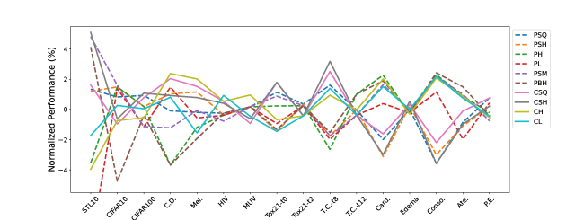
Figure 1: Loss functions comparisons on benchmark datasets (C.D for Cat vs Dog, Mel for Melanoma, T.C. for ToxCast, Card. for Cardiomegaly, Conso. for Consolidation, Ate. for Atelectasis, P.E. for Pleural Effusion. The percentages are normalized with the mean test AUROC of each data for all losses.)

As we can see from the results in Table 4, most of the data favors higher SPR than lower SPR. The phenomenon is more obvious on the generated image dataset. The observation indicates over-sampling positive data in the mini-batch could improve the AUROC optimization performance especially when testing data is more balanced.

The impact of CER. For CER, following (Yuan et al., 2020), we investigate three different values for $\gamma$: 0, 0.002, and 0.02. We fix other hyper-parameters as in the previous SPR setting and fix SPR as 50%. The results are presented in the Table 5. From the results, we can see CER generally improves the generalization performance for the image datasets. However, for some datasets that are more imbalanced, such as MUV(bioassay) with 0.2% positive rate and ToxCast(t12) with 3.0% positive rate, large CER could degrade model performance badly.

The impact of WD. The weight decay (WD) is tuned at {1e-1, 1e-2, 1e-3, 1e-4, 0}. The other hyper-parameters are fixed as in previous CER setting, except we now fix $\gamma$ in CER as 0.002 for image datasets and fix $\gamma$ in CER as 0 for molecule datasets as these two extremely imbalanced datasets don’t favor CER. The results are at appendix, as the observations are standard. Weight decay is generally believed to improve model generalization; it should be tuned in practice for different datasets.

The impact of activation/normalization. Next, we further fix WD as 1e-4, and tune the activation/normalization function for the output (last) layer as: none, sigmoid, $\ell_{1}$ score normalization, $\ell_{2}$ score normalization, and batch normalization. Because $\ell_{1}$ score normalization and batch-normalization are not so competitive as others, we omit them in the main content and show partial results in Table 6, which indicates that normalization is effective. The full results are included at appendix. We can see that the sigmoid activation and the $\ell_{2}$ norm score normalization are competitive and the former one wins more cases.

The impact of optimizers. Next, we fix last normalization function as sigmoid and conduct experiments on different optimizers from {SGD-style, Momentum-style, Adam-style} with different learning rates tuned from {1e-1, 1e-2, 1e-3, 1e-4, 1e-5}. The other settings are inherited as previous choices, that is, 50% for SPR, 0.002 for CER and 1e-4 for weight decay. The results are presented in Table 7. We also include the best learning rate with the optimizers at the appendix. The SGD and Momentum method perform well for all datasets; Adam optimizer doesn’t enjoy good testing performance, although it enjoys faster empirical training convergence speed, which we will elaborate shortly in subsection 3.4.

We also include the performance of the method PESG for solving the CSQ in the min-max form as used in (Yuan et al., 2020). It is notable that PESG uses a primal-dual stochastic gradient style update for solving the min-max form. The SGD-style optimizer for solving the composite form is equivalent to a primal-dual style update according to (Zhang and Lan, 2021). Neverthess, we can see that the SGD-style update for solving the composite form is better than PESG in more cases. This is probably due to another key difference between them, which is that PESG adopts random sampling while other three optimizers adopts the oversampling strategy. The observations are consistent with the previous observation for CSQ loss for SPR (sampling positive rate) study Table 4. For example, MUV, HIV and Cardiomegaly don’t necessarily require oversampling, where PESG enjoys better performance.

3.3 Pairwise Losses vs Composite Losses

Now that we get prior knowledge for the hyper-parameters, we conduct the final comparison for all loss functions of pairwise loss and composite loss classes. For all datasets except CheXpert, we choose the best hyper-parameters by validation AUROC produced by the above simplified sequential hyper-parameter tuning steps (SPR$\rightarrow$CER$\rightarrow$WD$\rightarrow$normalization/activation
$\rightarrow$optimizer) for PSQ and CSQ losses, whose details are included in the appendix. The results are presented at Figure 1. From the results, although there is no clear winner, composite loss outperforms classical pairwise loss on most of the datasets.

For all the targets at CheXpert dataset, we choose the hyper-parameters by prior knowledge on the other benchmark datasets, namely, SPR=50%, CER with $\gamma=0.002$, WD=1e-4, last activation as $\ell_{2}$-normalization, momentum-style optimizer with a learning rate of 1e-3. The choices are also close to the best choices based on the validation results for CheXpert Cardiomegaly under the simplified sequential tuning process. The results for CheXpert dataset are also presented at Figure 1. We include the detailed numerical tabular results for all benchmark datasets at Table 9, 10, 11.

All the five targets for CheXpert have uncertain labels and missing labels. The rates are shown in Table 8. Consolidation and Atelectasis are the two targets with highest uncertain rate; and they also have high missing rate. From the results in Table 11 in the appendix, the pairwise barrier hinge loss achieves the best performance and pairwise sigmoid loss also achieves good performance, which confirms the point that a symmetric loss is better under the learning with corrupted labels (Charoenphakdee et al., 2019).

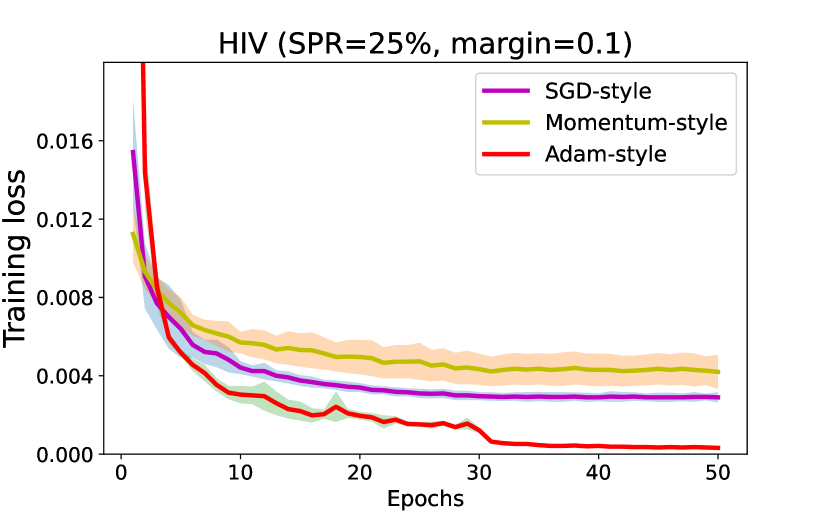
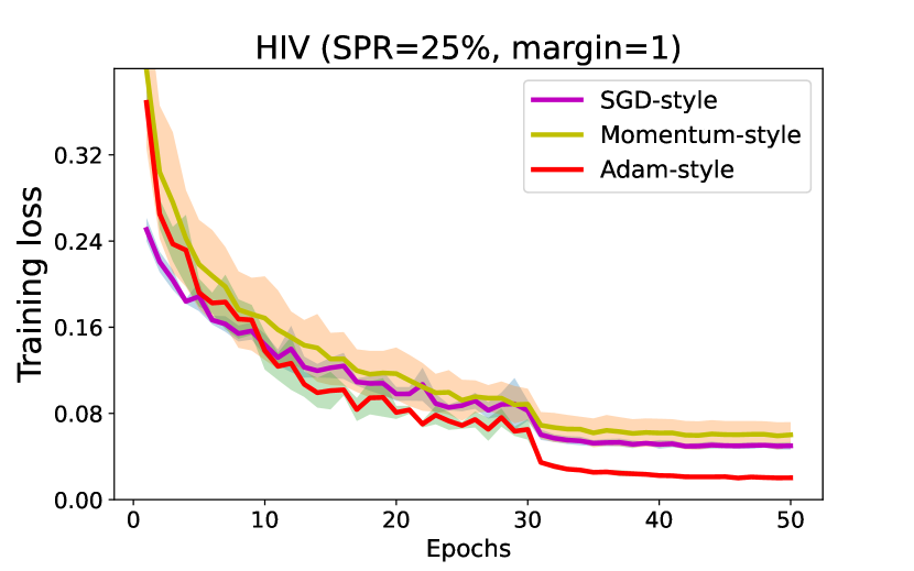
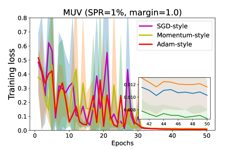
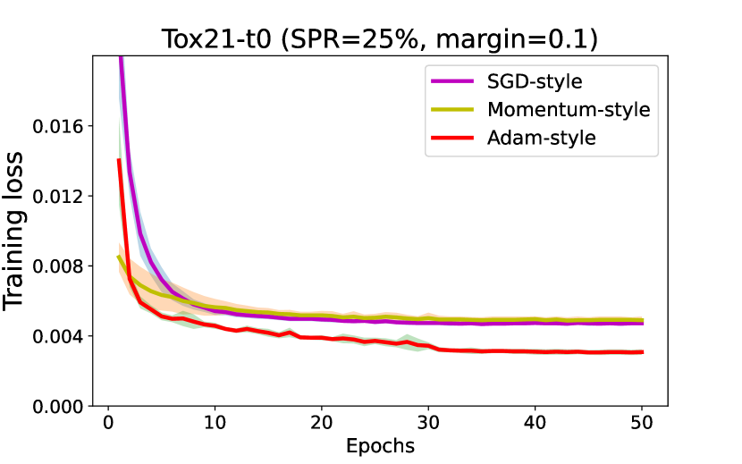
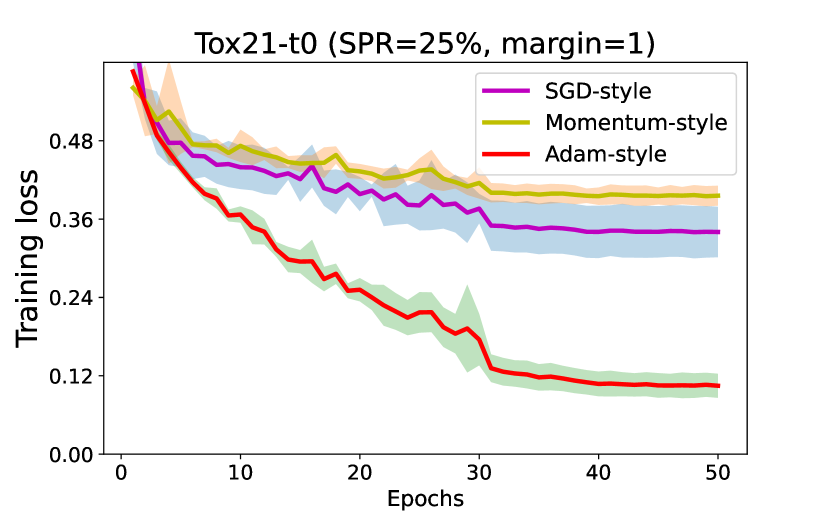
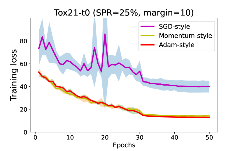
Figure 2: Different Optimizers for Composite Squared Hinge (CSH) Loss on Benchmark Datasets

Table 9: Different loss functions on image datasets

	Dataset	STL10	CIFAR10	CIFAR100	Cat vs Dog	Melanoma
	PSQ	0.727(0.031)	0.904(0.004)	0.683(0.003)	0.890(0.011)	0.810(0.013)
	PSH	0.726(0.031)	0.910(0.003)	0.678(0.005)	0.900(0.002)	0.821(0.014)
Pairwise	PH	0.692(0.056)	0.910(0.001)	0.678(0.008)	0.858(0.006)	0.802(0.015)
Loss	PL	0.653(0.070)	0.909(0.012)	0.669(0.013)	0.904(0.012)	0.807(0.016)
	PSM	0.752(0.025)	0.911(0.004)	0.669(0.014)	0.880(0.011)	0.811(0.014)
	PBH	0.747(0.017)	0.854(0.019)	0.674(0.014)	0.858(0.023)	0.796(0.017)
	CSQ	0.729(0.020)	0.888(0.014)	0.682(0.009)	0.909(0.011)	0.824(0.011)
Composite	CSH	0.754(0.033)	0.891(0.006)	0.684(0.005)	0.899(0.007)	0.818(0.013)
Loss	CH	0.689(0.052)	0.890(0.016)	0.673(0.024)	0.912(0.009)	0.828(0.002)
	CL	0.705(0.062)	0.899(0.004)	0.677(0.012)	0.898(0.010)	0.799(0.015)

Table 10: Different loss functions on molecular datasets

	Dataset	HIV	MUV(bioassay)	Tox21(t0)	Tox21(t2)	ToxCast(t8)	ToxCast(t12)
	PSQ	0.761(0.001)	0.639(0.001)	0.779(0.004)	0.901(0.002)	0.453(0.027)	0.573(0.016)
	PSH	0.760(0.002)	0.639(0.001)	0.759(0.002)	0.901(0.002)	0.438(0.013)	0.573(0.016)
Pairwise	PH	0.760(0.002)	0.639(0.001)	0.772(0.002)	0.900(0.001)	0.434(0.003)	0.579(0.008)
Loss	PL	0.760(0.003)	0.639(0.001)	0.763(0.012)	0.900(0.001)	0.437(0.008)	0.571(0.018)
	PSM	0.757(0.001)	0.639(0.001)	0.777(0.001)	0.900(0.001)	0.438(0.003)	0.571(0.018)
	PBH	0.761(0.002)	0.639(0.001)	0.760(0.008)	0.900(0.003)	0.439(0.011)	0.579(0.014)
	CSQ	0.767(0.002)	0.632(0.008)	0.784(0.007)	0.894(0.001)	0.457(0.012)	0.571(0.017)
Composite	CSH	0.766(0.002)	0.634(0.008)	0.784(0.007)	0.894(0.001)	0.460(0.011)	0.571(0.017)
Loss	CH	0.767(0.007)	0.644(0.008)	0.765(0.004)	0.894(0.001)	0.450(0.005)	0.573(0.016)
	CL	0.770(0.004)	0.635(0.009)	0.759(0.001)	0.894(0.002)	0.452(0.005)	0.571(0.017)

Table 11: Different loss functions on CheXpert dataset

	Dataset	Cardiomegaly(t0)	Edema(t1)	Consolidation(t2)	Atelectasis(t3)	Pleural Effusion(t4)
	PSQ	0.782(0.011)	0.922(0.006)	0.836(0.016)	0.800(0.007)	0.927(0.002)
	PSH	0.773(0.025)	0.924(0.004)	0.841(0.028)	0.798(0.021)	0.922(0.007)
Pairwise	PH	0.816(0.006)	0.919(0.002)	0.887(0.010)	0.814(0.004)	0.918(0.002)
Loss	PL	0.801(0.005)	0.920(0.003)	0.877(0.016)	0.791(0.002)	0.924(0.001)
	PSM	0.811(0.005)	0.921(0.001)	0.886(0.013)	0.815(0.005)	0.913(0.003)
	PBH	0.813(0.005)	0.920(0.001)	0.888(0.009)	0.819(0.003)	0.916(0.001)
	CSQ	0.785(0.013)	0.925(0.004)	0.848(0.022)	0.806(0.006)	0.927(0.005)
Composite	CSH	0.774(0.025)	0.927(0.003)	0.836(0.019)	0.799(0.015)	0.922(0.007)
Loss	CH	0.814(0.004)	0.919(0.001)	0.885(0.010)	0.814(0.004)	0.915(0.002)
	CL	0.810(0.005)	0.922(0.001)	0.886(0.008)	0.813(0.004)	0.916(0.002)

3.4 Numerical Analysis of Optimizers

We compare different styles of optimizers for optimizing CSH loss, namely PESG (Yuan et al., 2020), the momentum-style (Ghadimi et al., 2020), and the Adam-style (Wang et al., 2021). The learning rates are tuned from {1e-1, 1e-2, 1e-3, 1e-4, 1e-5}. Partial training convergence curves are presented in Figure 2. Full results are included in the appendix. The results show that the Adam-style optimizer is more competitive than other optimizers for solving the composite loss from the training perspective. The observation is especially strong for the molecule graph datasets. However, as we check the testing performance in Table 7, the Adam-style optimizer does not show better testing performance. The findings confirm that adaptive optimizer doesn’t have good generalization performance from the previous research (Wilson et al., 2017). We also compare the training convergence for composite loss v.s. pairwise loss at appendix. Overall, composite loss is more competitive for training convergence versus iteration number. Moreover, composite loss consumes smaller running time for each iteration.

4 Limitations and Conclusions

The limitation for this study is that we did not exhaustively search all the settings of different algorithmic factors for deep AUROC optimization due to the computational cost. However, based on our carefully designed experiments, we gain three insights for deep AUROC maximization from the perspective of loss functions, algorithmic choices and optimizers: (i) composite loss performs well and data with corrupted labels favors a symmetric pairwise loss; (2) some algorithmic choices such as over-sampling and normalization are helpful for deep AUROC maximization; (iii) Adam-type optimizer performs well on training data but not testing data. We expect these findings will be useful for future research and development on deep AUROC maximization.

Appendix A More Experiments for Test AUROC

A.1 Weight Decay

All test AUROC results for different weight decays are included at Table 12.

A.2 Normalization for Last Layer

All test AUROC results for normalization functions of last layer are included at Table 13.

A.3 Optimizers with Best Learning Rates

All test AUROC results for optimiers (SGD, Momentum, Adam type) and their learning rates (from {1e-1,1e-2,1e-3,1e-4,1e-5}) are included at Table 14.

A.4 Test AUROC for Loss Functions

The final comprehensive evaluation of all loss functions for image dataset, molecule dataset and specifically CheXpert dataset are included at Table 9, Table 10 and Table 11.

Appendix B More Experiments for Validation AUROC

B.1 Sampling positive rate

We include the sampling positive rate with validation AUROC at Table 15. Similar with test AUROC, over-sampling also improve validation AUROC.

B.2 Consecutive Epoch Regularization

We include the consecutive epoch regularization with validation AUROC at Table 16, where we see CER could improve validation AUROC as well.

B.3 Weight Decay

We include the weight decay with validation AUROC at Table 17. Although most of the datasets favors WD with medium value for Validation AUROC. It is better to tune it for different datasets in practice.

B.4 Normalization for Last Layer

We include the normalization of last layer with validation AUROC at Table 18. Sigmoid function is the most competitive normalization function, which is also consistant with the test AUROC results.

B.5 Optimizers with Best Learning Rates

We include the optimizers performance with their best learning rates for validation AUROC at Table 19. As the test AUROC, Adam-type of optimizer doesn’t perform well for validation AUROC either.

Appendix C More Experiments for Training Convergence

C.1 Optimizers Comparison for CSH Loss

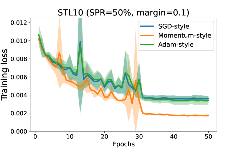
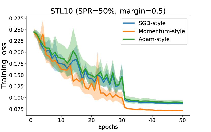
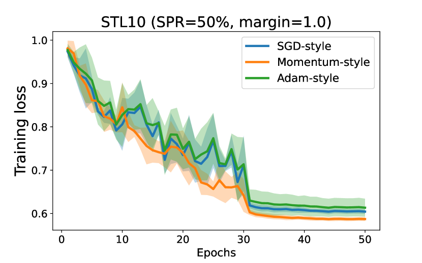
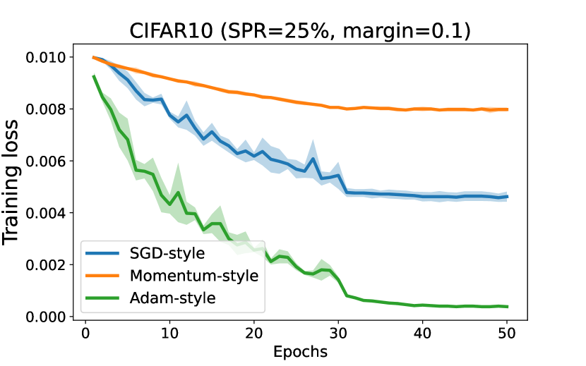
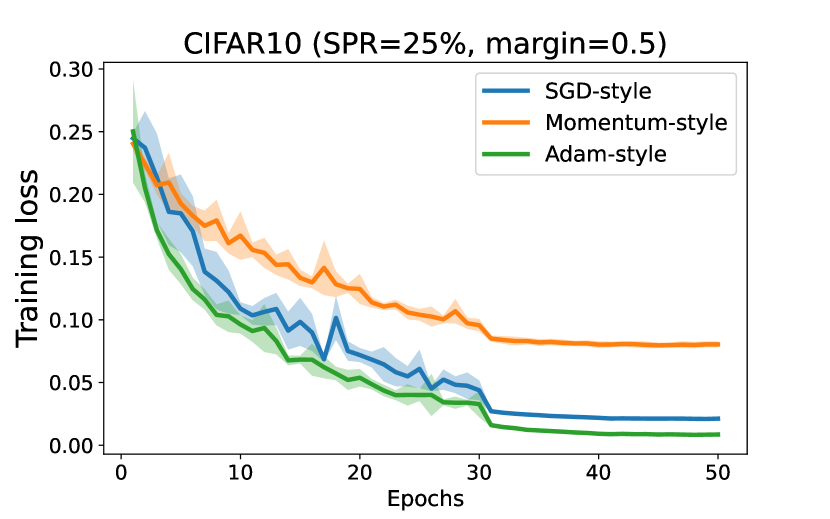
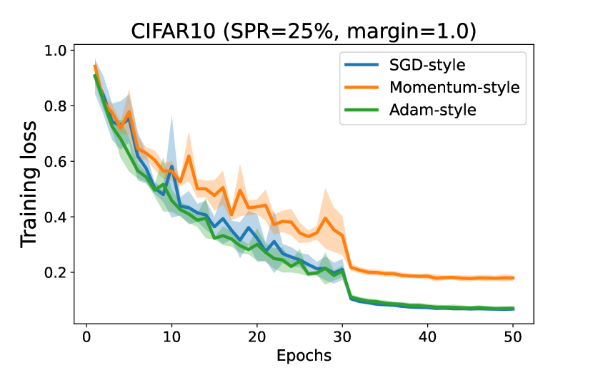
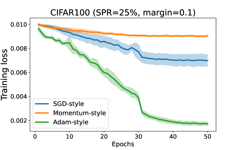
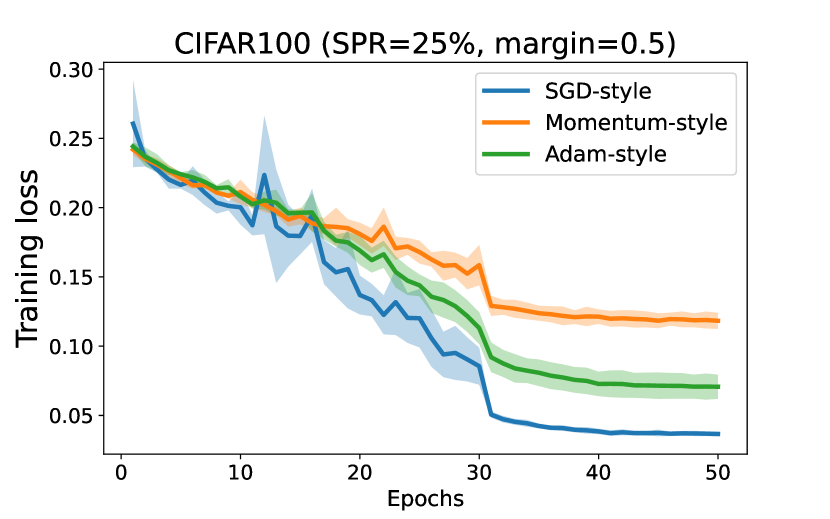
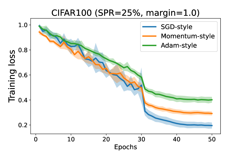
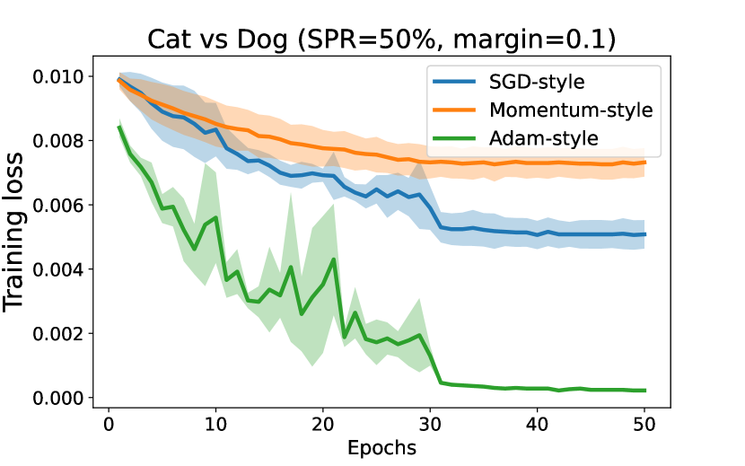
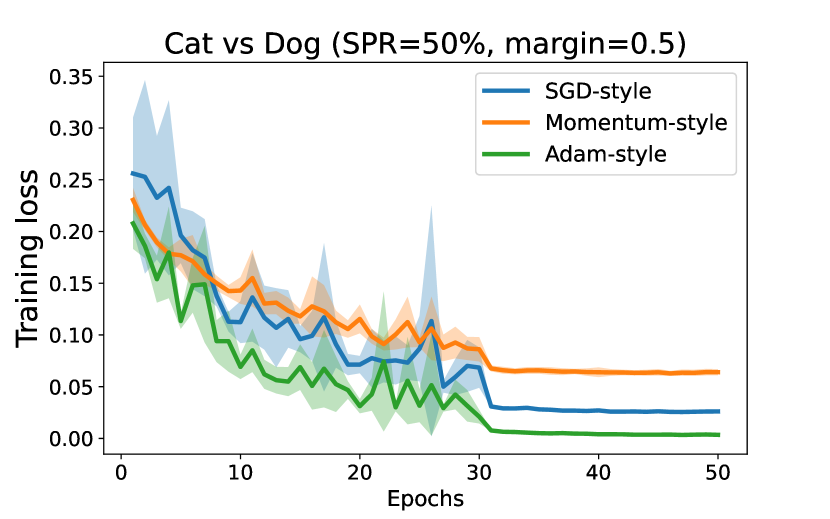
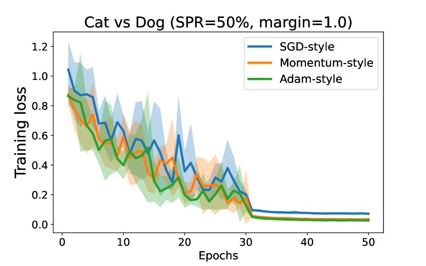
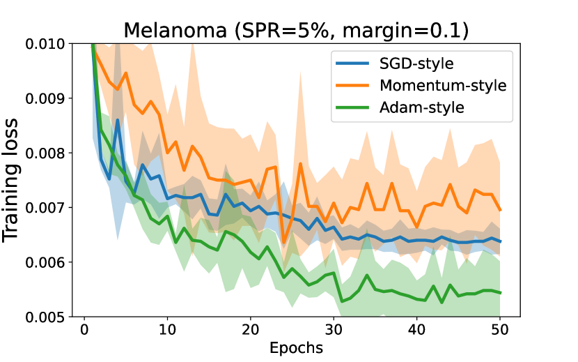
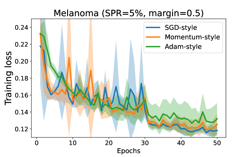
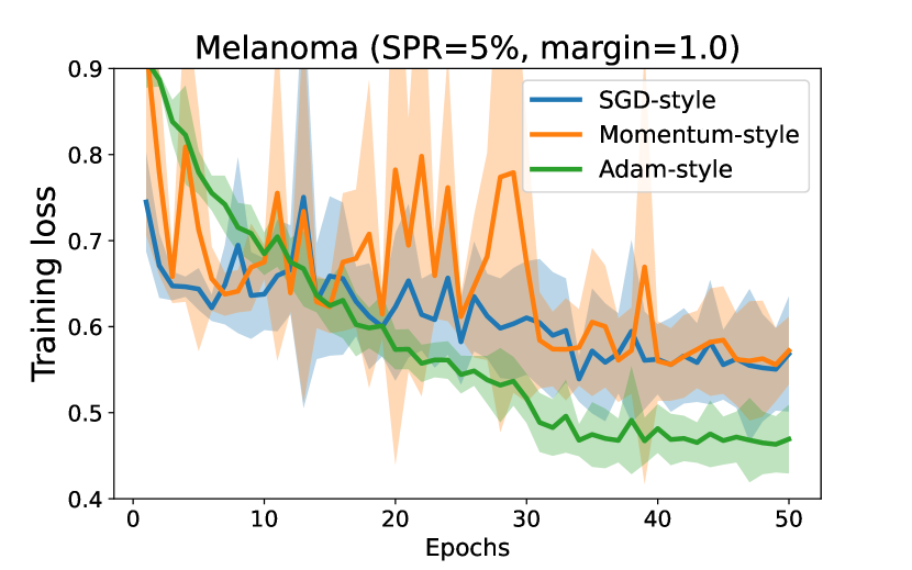
Figure 4: Different Optimizers for Composite Squared Hinge Loss on Image datasets

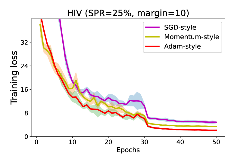
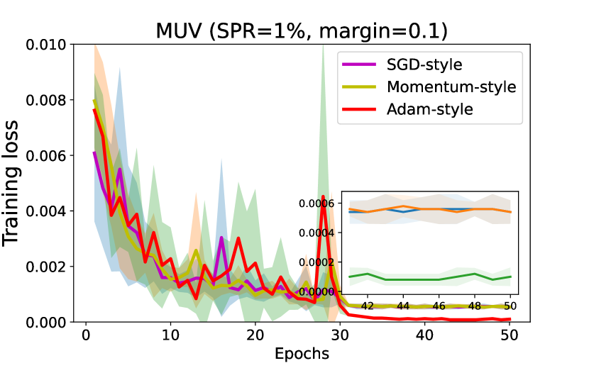
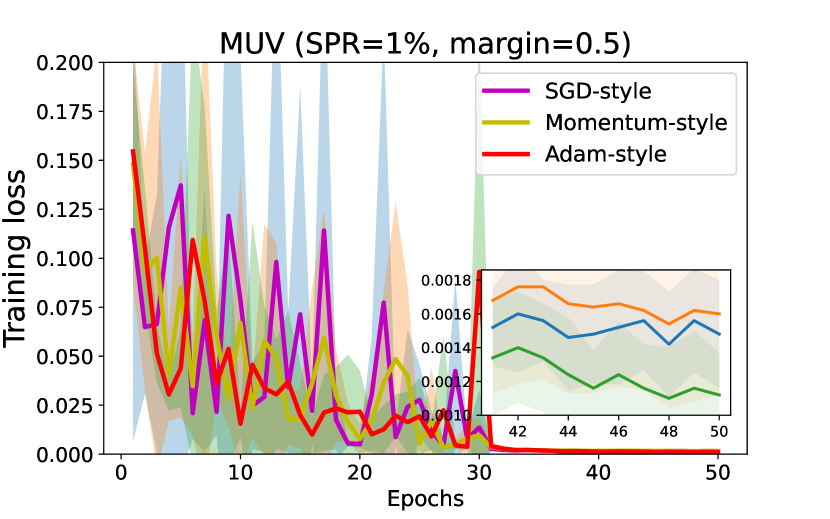
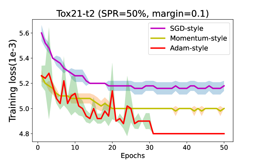
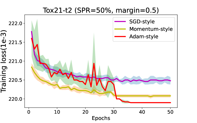
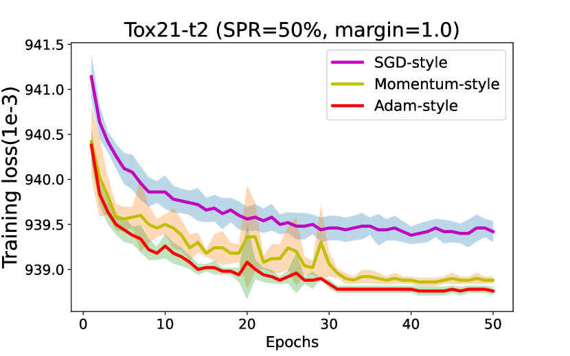
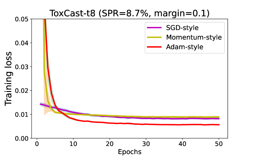
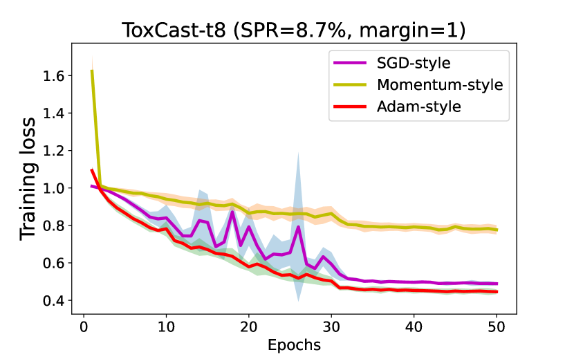
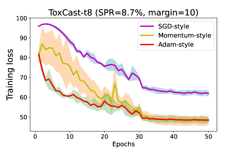
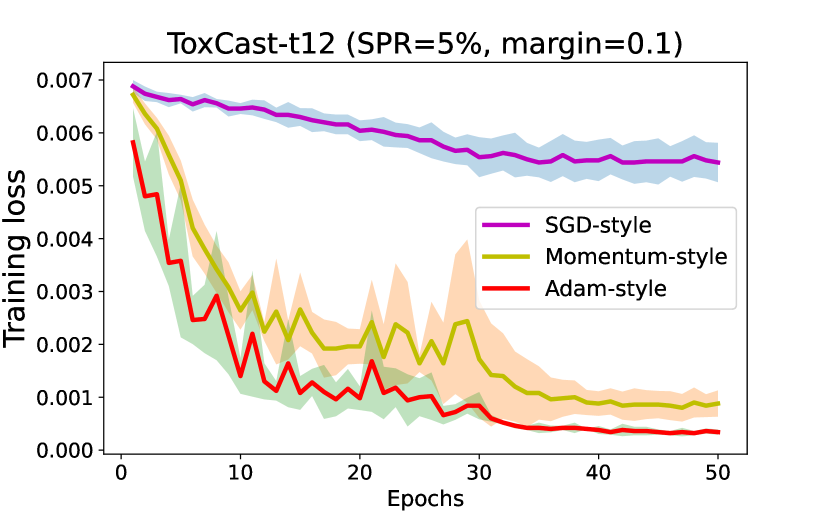
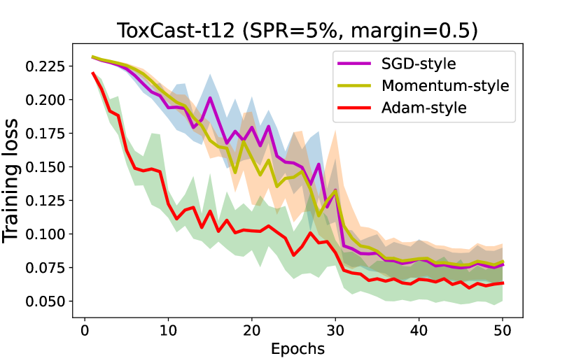
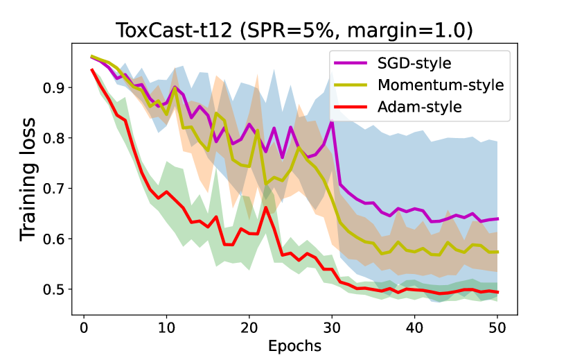
Figure 5: Different Optimizers for Composite Squared Hinge Loss on Molecule datasets

We include all the figures for optimizers (SGD, Momentum and Adam styles) for CSH loss at Figure 4 for image datasets and Figure 5 for molecule datasets. CAdam is the most competitive optimizer for all the datasets, and even achieve dominating performance for molecule datasets from the training convergence perspective. However, as emphasized at the main content, the drawback for CAdam is it doesn’t generalize well.

C.2 Optimization: PSQ v.s. CSQ

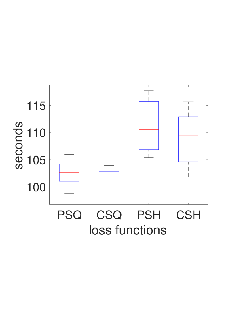
Figure 3: Time Consuming for every 40 iterations

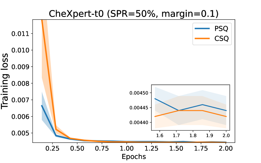
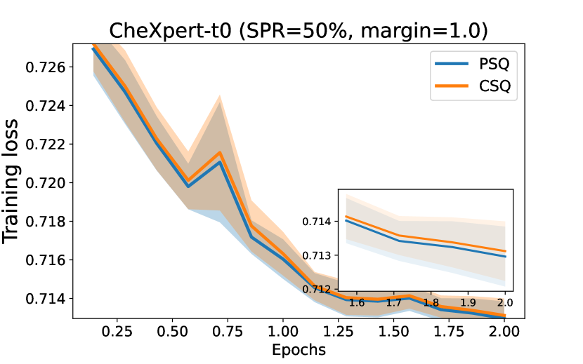
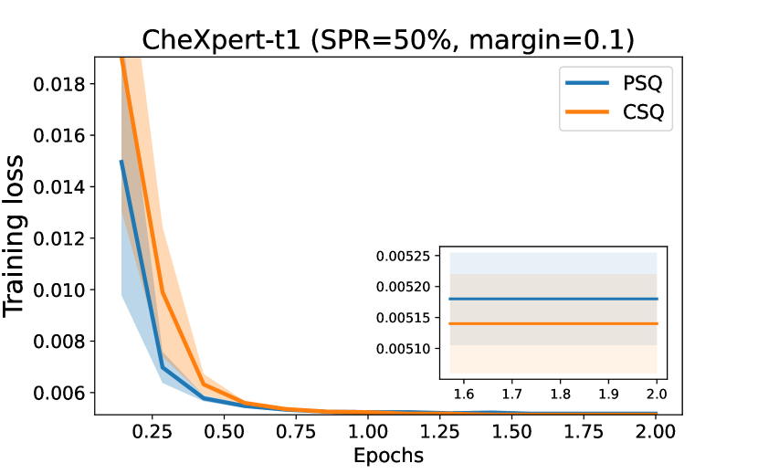
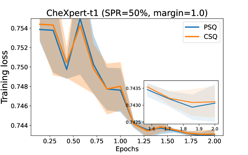
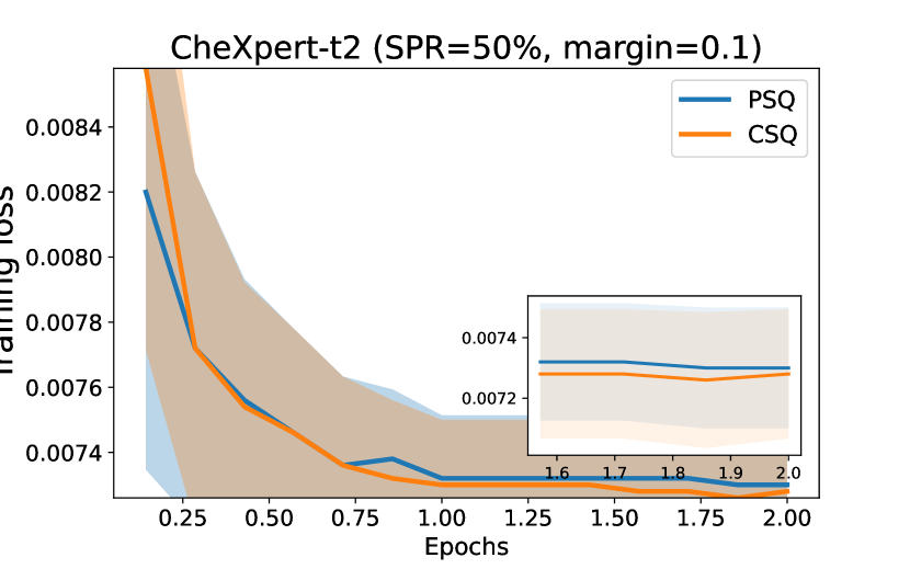
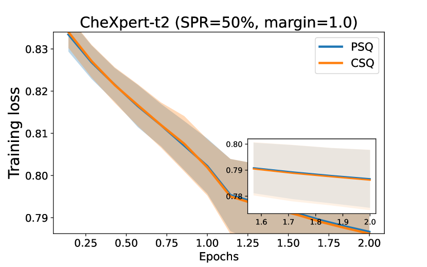
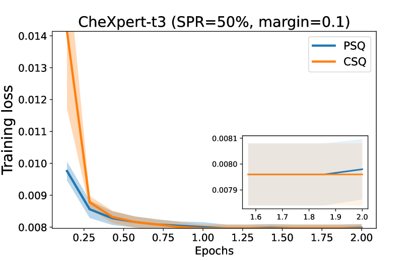
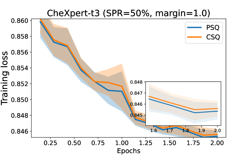
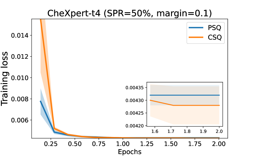
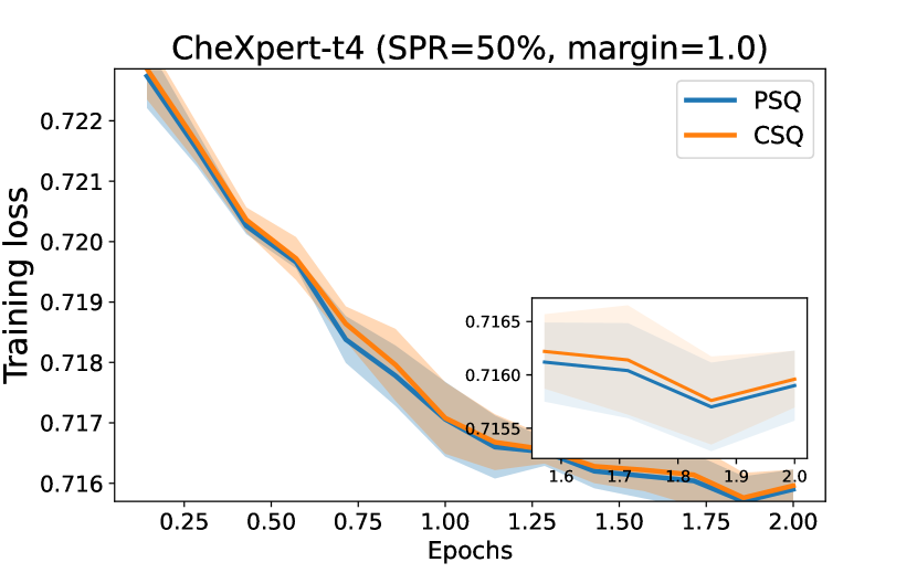
Figure 6: PSQ v.s. CSQ on CheXpert dataset

Because PSQ and CSQ are proved equivalent Ying et al. (2016), we may wonder which one is better only from the optimization perspective. To this purpose, we compare them under sigmoid normalization for last layer, momentum optimizer with learning rate as 1e-3. We include the training convergence for PSQ and CSQ loss on CheXpert dataset for the five targets, t0: Cardiomegaly, t1: Edema, t2: Consolidation, t3: Atelectasis, t4: Pleural Effusion, at Figure 6. From the results, we can see CSQ is clearly better than PSQ for smaller margin parameter (0.1), but slightly worse when margin is larger (1.0). To this end, we investigate the running time for PSQ v.s. CSQ, and PSH v.s. CSH because they are equivalent as well. We count the running time under GeForce GTX 1080 Ti Graphics Card for every 40 iterations of mini-batch of 64 at Figure 3, where We repeat the counting independently for 20 times. Both CSQ and CSH are faster than PSQ and PSH, which could due to pairwise loss need generate all pairs inside of mini-batch.

Table 12: Weight decay with testing AUROC

Loss	Dataset	WD$=1e-1$	WD$=1e-2$	WD$=1e-3$	WD$=1e-4$	WD$=0$
	STL10	0.761(0.040)	0.793(0.013)	0.772(0.023)	0.761(0.014)	0.780(0.019)
	CIFAR10	0.620(0.010)	0.899(0.002)	0.911(0.001)	0.907(0.002)	0.907(0.002)
	CIFAR100	0.549(0.007)	0.652(0.025)	0.681(0.006)	0.669(0.011)	0.678(0.008)
	Cat vs Dog	0.688(0.010)	0.945(0.004)	0.932(0.003)	0.930(0.004)	0.927(0.007)
	Melanoma	0.719(0.014)	0.802(0.012)	0.794(0.013)	0.798(0.012)	0.806(0.019)
	Cardiomegaly	0.841(0.007)	0.835(0.006)	0.826(0.005)	0.832(0.007)	0.828(0.006)
PSQ	HIV	0.753(0.021)	0.753(0.015)	0.758(0.007)	0.759(0.014)	0.750(0.008)
	MUV(bioassay)	0.518(0.060)	0.563(0.089)	0.651(0.102)	0.638(0.033)	0.627(0.050)
	tox21(t0)	0.743(0.011)	0.748(0.015)	0.742(0.009)	0.747(0.005)	0.746(0.008)
	tox21(t2)	0.881(0.009)	0.885(0.013)	0.881(0.012)	0.880(0.016)	0.889(0.006)
	toxcast(t8)	0.490(0.024)	0.484(0.025)	0.492(0.025)	0.497(0.029)	0.496(0.032)
	toxcast(t12)	0.734(0.167)	0.640(0.214)	0.673(0.243)	0.676(0.236)	0.642(0.217)
	STL10	0.669(0.099)	0.795(0.010)	0.751(0.045)	0.727(0.064)	0.729(0.078)
	CIFAR10	0.564(0.037)	0.893(0.010)	0.908(0.004)	0.902(0.005)	0.907(0.005)
	CIFAR100	0.551(0.012)	0.665(0.006)	0.676(0.010)	0.680(0.008)	0.684(0.006)
	Cat vs Dog	0.668(0.029)	0.943(0.004)	0.930(0.006)	0.926(0.008)	0.920(0.004)
	Melanoma	0.714(0.008)	0.782(0.022)	0.798(0.013)	0.802(0.019)	0.783(0.017)
	Cardiomegaly	0.838(0.015)	0.833(0.005)	0.832(0.005)	0.833(0.005)	0.832(0.006)
CSQ	HIV	0.763(0.015)	0.766(0.016)	0.763(0.015)	0.747(0.012)	0.741(0.012)
	MUV(bioassay)	0.579(0.092)	0.629(0.073)	0.689(0.056)	0.702(0.092)	0.659(0.071)
	tox21(t0)	0.761(0.016)	0.756(0.016)	0.758(0.019)	0.757(0.016)	0.760(0.020)
	tox21(t2)	0.887(0.009)	0.887(0.009)	0.881(0.012)	0.890(0.006)	0.892(0.005)
	toxcast(t8)	0.487(0.030)	0.479(0.027)	0.487(0.023)	0.470(0.030)	0.476(0.022)
	toxcast(t12)	0.708(0.160)	0.727(0.152)	0.746(0.111)	0.740(0.109)	0.723(0.152)

Table 13: Normalization function for prediction layer with testing AUROC

Loss	Dataset	None	sigmoid	$\ell_{1}$-normalization	$\ell_{2}$-normalization	batch normalization
	STL10	0.726(0.030)	0.772(0.023)	0.734(0.012)	0.769(0.006)	0.747(0.020)
	CIFAR10	0.900(0.005)	0.911(0.001)	0.853(0.004)	0.893(0.006)	0.893(0.009)
	CIFAR100	0.660(0.012)	0.681(0.007)	0.669(0.014)	0.683(0.006)	0.667(0.002)
	Cat vs Dog	0.895(0.036)	0.932(0.003)	0.824(0.030)	0.919(0.004)	0.922(0.005)
	Melanoma	0.793(0.035)	0.794(0.013)	0.780(0.011)	0.810(0.011)	0.805(0.010)
	Cardiomegaly	0.800(0.010)	0.832(0.007)	0.832(0.007)	0.815(0.030)	0.832(0.007)
PSQ	HIV	0.760(0.010)	0.734(0.031)	0.731(0.013)	0.745(0.006)	0.755(0.019)
	MUV(bioassay)	0.579(0.101)	0.598(0.063)	0.603(0.034)	0.604(0.049)	0.580(0.194)
	Tox21(t0)	0.744(0.008)	0.782(0.004)	0.772(0.017)	0.768(0.017)	0.738(0.014)
	Tox21(t2)	0.883(0.009)	0.883(0.012)	0.886(0.006)	0.888(0.008)	0.886(0.015)
	ToxCast(t8)	0.518(0.051)	0.500(0.040)	0.469(0.025)	0.477(0.068)	0.481(0.031)
	ToxCast(t12)	0.735(0.170)	0.840(0.104)	0.590(0.052)	0.613(0.054)	0.617(0.105)
	STL10	0.656(0.079)	0.751(0.046)	0.698(0.019)	0.763(0.011)	0.746(0.021)
	CIFAR10	0.781(0.048)	0.908(0.004)	0.853(0.006)	0.894(0.006)	0.898(0.003)
	CIFAR100	0.631(0.025)	0.676(0.010)	0.676(0.006)	0.675(0.007)	0.670(0.004)
	Cat vs Dog	0.814(0.114)	0.929(0.006)	0.842(0.023)	0.916(0.009)	0.917(0.010)
	Melanoma	0.801(0.015)	0.798(0.013)	0.788(0.015)	0.811(0.013)	0.799(0.029)
	Cardiomegaly	0.809(0.015)	0.833(0.005)	0.833(0.005)	0.814(0.024)	0.830(0.005)
CSQ	HIV	0.756(0.019)	0.744(0.017)	0.734(0.012)	0.741(0.008)	0.756(0.006)
	MUV(bioassay)	0.639(0.091)	0.599(0.063)	0.641(0.072)	0.578(0.107)	0.597(0.103)
	Tox21(t0)	0.756(0.018)	0.755(0.005)	0.754(0.035)	0.773(0.014)	0.750(0.023)
	Tox21(t2)	0.889(0.004)	0.895(0.005)	0.887(0.003)	0.892(0.008)	0.886(0.006)
	ToxCast(t8)	0.490(0.033)	0.523(0.065)	0.456(0.034)	0.483(0.047)	0.499(0.055)
	ToxCast(t12)	0.721(0.150)	0.985(0.008)	0.585(0.042)	0.769(0.061)	0.660(0.092)

Table 14: Optimizers with testing AUROC

Loss	Dataset	SGD-style	Momentum-style	Adam-style
	STL10	0.771(0.007)	0.803(0.015)	0.794(0.011)
	CIFAR10	0.909(0.002)	0.911(0.001)	0.868(0.004)
	CIFAR100	0.688(0.002)	0.681(0.007)	0.669(0.011)
	Cat vs Dog	0.937(0.004)	0.932(0.003)	0.902(0.010)
	Melanoma	0.804(0.024)	0.801(0.009)	0.810(0.015)
	Cardiomegaly	0.848(0.005)	0.848(0.005)	0.853(0.009)
PSQ	HIV	0.767(0.005)	0.767(0.005)	0.766(0.002)
	MUV(bioassay)	0.690(0.030)	0.703(0.030)	0.702(0.053)
	Tox21(t0)	0.788(0.005)	0.788(0.005)	0.752(0.011)
	Tox21(t2)	0.903(0.002)	0.904(0.001)	0.893(0.004)
	ToxCast(t8)	0.444(0.018)	0.460(0.104)	0.553(0.056)
	ToxCast(t12)	0.908(0.036)	0.908(0.047)	0.910(0.040)
	STL10	1e-1	1e-1	1e-3
	CIFAR10	1e-1	1e-2	1e-3
	CIFAR100	1e-1	1e-2	1e-4
	Cat vs Dog	1e-1	1e-3	1e-3
	Melanoma	1e-2	1e-3	1e-4
	Cardiomegaly	1e-4	1e-5	1e-3
PSQ	HIV	1e-4	1e-5	1e-4
	MUV(bioassay)	1e-1	1e-2	1e-3
	Tox21(t0)	1e-4	1e-5	1e-3
	Tox21(t2)	1e-3	1e-4	1e-4
	ToxCast(t8)	1e-2	1e-1	1e-2
	ToxCast(t12)	1e-2	1e-3	1e-4

Loss	Dataset	SGD-style	Momentum-style	Adam-style	PESG
	STL10	0.796(0.013)	0.819(0.003)	0.785(0.016)	0.766(0.020)
	CIFAR10	0.910(0.002)	0.905(0.006)	0.845(0.023)	0.886(0.007)
	CIFAR100	0.678(0.010)	0.684(0.005)	0.652(0.007)	0.664(0.006)
	Cat vs Dog	0.934(0.006)	0.930(0.004)	0.907(0.008)	0.916(0.006)
	Melanoma	0.803(0.020)	0.818(0.004)	0.812(0.009)	0.815(0.016)
	Cardiomegaly	0.861(0.004)	0.862(0.004)	0.840(0.012)	0.861(0.004)
CSQ	HIV	0.770(0.003)	0.770(0.003)	0.763(0.005)	0.775(0.007)
	MUV(bioassay)	0.715(0.040)	0.699(0.026)	0.684(0.084)	0.721(0.049)
	Tox21(t0)	0.779(0.002)	0.777(0.017)	0.781(0.012)	0.778(0.003)
	Tox21(t2)	0.898(0.003)	0.899(0.002)	0.893(0.007)	0.898(0.007)
	ToxCast(t8)	0.445(0.009)	0.499(0.002)	0.467(0.055)	0.443(0.006)
	ToxCast(t12)	0.875(0.084)	0.883(0.047)	0.900(0.036)	0.821(0.044)
	STL10	1e-1	1e-1	1e-3	1e-1
	CIFAR10	1e-1	1e-2	1e-3	1e-1
	CIFAR100	1e-1	1e-2	1e-4	1e-2
	Cat vs Dog	1e-1	1e-3	1e-3	1e-1
	Melanoma	1e-1	1e-3	1e-5	1e-2
	Cardiomegaly	1e-4	1e-5	1e-4	1e-4
CSQ	HIV	1e-4	1e-5	1e-4	1e-4
	MUV(bioassay)	1e-1	1e-2	1e-3	1e-2
	Tox21(t0)	1e-5	1e-4	1e-3	1e-5
	Tox21(t2)	1e-3	1e-4	1e-3	1e-3
	ToxCast(t8)	1e-3	1e-1	1e-1	1e-4
	ToxCast(t12)	1e-2	1e-3	1e-4	1e-2

Table 15: Sampling positive rate with validation AUROC

Loss	Dataset	PR$=$origin	PR$=5\%$	PR$=25\%$	PR$=50\%$
	STL10	0.776(0.030)	0.724(0.014)	0.809(0.027)	0.810(0.027)
	CIFAR10	0.916(0.018)	0.884(0.008)	0.930(0.015)	0.928(0.013)
	CIFAR100	0.725(0.011)	0.715(0.021)	0.749(0.030)	0.740(0.018)
	Cat vs Dog	0.912(0.015)	0.887(0.015)	0.928(0.012)	0.924(0.012)
	Melanoma	0.764(0.014)	0.803(0.010)	0.802(0.021)	0.802(0.015)
	Cardiomegaly	0.873(0.002)	0.872(0.002)	0.874(0.002)	0.875(0.002)
PSQ	HIV	0.875(0.028)	0.879(0.034)	0.890(0.034)	0.891(0.036)
	MUV	0.929(0.050)	0.902(0.046)	0.914(0.053)	0.912(0.060)
	tox21(t0)	0.861(0.013)	0.862(0.015)	0.868(0.020)	0.870(0.020)
	tox21(t2)	0.954(0.009)	0.952(0.010)	0.957(0.011)	0.955(0.007)
	toxcast(t8)	0.840(0.031)	0.838(0.040)	0.847(0.036)	0.844(0.030)
	toxcast(t12)	0.950(0.029)	0.948(0.040)	0.933(0.055)	0.935(0.056)
	STL10	0.680(0.088)	0.634(0.077)	0.699(0.113)	0.705(0.107)
	CIFAR10	0.871(0.062)	0.849(0.047)	0.898(0.048)	0.893(0.052)
	CIFAR100	0.726(0.020)	0.692(0.028)	0.731(0.017)	0.721(0.023)
	Cat vs Dog	0.812(0.065)	0.864(0.040)	0.775(0.094)	0.891(0.030)
	Melanoma	0.771(0.023)	0.802(0.021)	0.795(0.018)	0.796(0.020)
	Cardiomegaly	0.872(0.002)	0.871(0.002)	0.874(0.002)	0.876(0.002)
CSQ	HIV	0.862(0.035)	0.874(0.033)	0.886(0.032)	0.873(0.025)
	MUV	0.918(0.058)	0.906(0.068)	0.899(0.068)	0.893(0.064)
	tox21(t0)	0.857(0.016)	0.859(0.015)	0.876(0.016)	0.874(0.022)
	tox21(t2)	0.957(0.009)	0.951(0.010)	0.958(0.009)	0.960(0.009)
	toxcast(t8)	0.839(0.031)	0.837(0.039)	0.834(0.034)	0.837(0.042)
	toxcast(t12)	0.965(0.043)	0.972(0.038)	0.964(0.045)	0.962(0.052)

Table 16: Consecutive epoch regularization with validation AUROC

Loss	Dataset	$\gamma=0$	$\gamma=0.002$	$\gamma=0.02$
	STL10	0.810(0.027)	0.817(0.033)	0.829(0.019)
	CIFAR10	0.928(0.013)	0.945(0.012)	0.937(0.005)
	CIFAR100	0.740(0.018)	0.744(0.020)	0.706(0.013)
	Cat vs Dog	0.924(0.012)	0.940(0.009)	0.950(0.008)
	Melanoma	0.802(0.015)	0.797(0.012)	0.806(0.019)
PSQ	Cardiomegaly	0.874(0.002)	0.876(0.002)	0.877(0.002)
	HIV	0.891(0.036)	0.885(0.035)	0.873(0.023)
	MUV	0.912(0.061)	0.915(0.053)	0.909(0.046)
	tox21(t0)	0.870(0.020)	0.868(0.022)	0.864(0.027)
	tox21(t2)	0.955(0.007)	0.954(0.006)	0.951(0.007)
	toxcast(t8)	0.844(0.030)	0.839(0.030)	0.847(0.039)
	toxcast(t12)	0.935(0.056)	0.936(0.057)	0.937(0.058)
	STL10	0.705(0.108)	0.741(0.068)	0.829(0.032)
	CIFAR10	0.893(0.052)	0.942(0.011)	0.932(0.007)
	CIFAR100	0.721(0.023)	0.741(0.012)	0.735(0.014)
	Cat vs Dog	0.891(0.030)	0.934(0.008)	0.947(0.007)
	Melanoma	0.796(0.020)	0.800(0.018)	0.805(0.018)
	Cardiomegaly	0.876(0.002)	0.876(0.002)	0.877(0.002)
CSQ	HIV	0.873(0.025)	0.875(0.026)	0.878(0.027)
	MUV	0.893(0.064)	0.901(0.064)	0.905(0.061)
	tox21(t0)	0.874(0.022)	0.873(0.022)	0.873(0.023)
	tox21(t2)	0.960(0.009)	0.958(0.007)	0.956(0.006)
	toxcast(t8)	0.837(0.042)	0.831(0.043)	0.842(0.024)
	toxcast(t12)	0.962(0.052)	0.961(0.053)	0.963(0.050)

Table 17: Weight decay with validation AUROC

Loss	Dataset	$WD=1e-1$	$WD=1e-2$	$WD=1e-3$	$WD=1e-4$	$WD=0$
	STL10	0.780(0.038)	0.834(0.019)	0.816(0.035)	0.817(0.033)	0.810(0.020)
	CIFAR10	0.645(0.012)	0.946(0.003)	0.946(0.008)	0.945(0.012)	0.943(0.008)
	CIFAR100	0.588(0.015)	0.735(0.022)	0.747(0.009)	0.745(0.020)	0.754(0.006)
	Cat vs Dog	0.724(0.008)	0.954(0.005)	0.944(0.011)	0.940(0.009)	0.939(0.011)
	Melanoma	0.728(0.017)	0.804(0.018)	0.795(0.018)	0.797(0.012)	0.803(0.017)
	Cardiomegaly	0.838(0.001)	0.877(0.002)	0.876(0.002)	0.876(0.002)	0.876(0.002)
PSQ	HIV	0.857(0.032)	0.877(0.032)	0.889(0.034)	0.891(0.036)	0.891(0.034)
	MUV	0.923(0.051)	0.918(0.049)	0.921(0.057)	0.912(0.061)	0.905(0.061)
	tox21(t0)	0.862(0.025)	0.865(0.025)	0.864(0.026)	0.870(0.020)	0.864(0.026)
	tox21(t2)	0.949(0.007)	0.953(0.006)	0.954(0.007)	0.955(0.007)	0.954(0.008)
	toxcast(t8)	0.841(0.031)	0.849(0.037)	0.843(0.036)	0.844(0.030)	0.848(0.036)
	toxcast(t12)	0.933(0.055)	0.937(0.058)	0.934(0.056)	0.935(0.056)	0.935(0.056)
	STL10	0.712(0.082)	0.815(0.022)	0.779(0.049)	0.741(0.068)	0.771(0.080)
	CIFAR10	0.586(0.033)	0.951(0.007)	0.946(0.008)	0.942(0.011)	0.949(0.010)
	CIFAR100	0.616(0.016)	0.727(0.015)	0.747(0.015)	0.741(0.012)	0.753(0.011)
	Cat vs Dog	0.702(0.022)	0.954(0.008)	0.936(0.013)	0.934(0.008)	0.927(0.016)
	Melanoma	0.728(0.022)	0.801(0.013)	0.808(0.015)	0.800(0.018)	0.798(0.014)
	Cardiomegaly	0.839(0.001)	0.877(0.002)	0.876(0.002)	0.876(0.002)	0.876(0.002)
CSQ	HIV	0.870(0.026)	0.872(0.029)	0.880(0.027)	0.872(0.025)	0.877(0.029)
	MUV	0.902(0.066)	0.901(0.062)	0.898(0.063)	0.893(0.064)	0.899(0.067)
	tox21(t0)	0.870(0.019)	0.874(0.022)	0.874(0.024)	0.874(0.022)	0.873(0.022)
	tox21(t2)	0.954(0.007)	0.959(0.010)	0.959(0.009)	0.960(0.009)	0.960(0.009)
	toxcast(t8)	0.830(0.033)	0.831(0.025)	0.838(0.032)	0.837(0.042)	0.838(0.037)
	toxcast(t12)	0.959(0.054)	0.961(0.052)	0.962(0.052)	0.962(0.052)	0.961(0.051)

Table 18: Normalization with validation AUROC

Loss	Dataset	None	sigmoid	$\ell_{1}$-normalization	$\ell_{2}$-normalization	batch normalization
	STL10	0.769(0.027)	0.816(0.035)	0.771(0.020)	0.812(0.023)	0.793(0.026)
	CIFAR10	0.932(0.014)	0.946(0.008)	0.898(0.005)	0.933(0.009)	0.931(0.012)
	CIFAR100	0.727(0.015)	0.747(0.009)	0.728(0.011)	0.754(0.008)	0.736(0.011)
	Cat vs Dog	0.899(0.028)	0.944(0.011)	0.856(0.023)	0.922(0.010)	0.926(0.011)
	Melanoma	0.796(0.016)	0.795(0.018)	0.790(0.014)	0.794(0.014)	0.789(0.016)
	Cardiomegaly	0.876(0.001)	0.876(0.002)	0.876(0.002)	0.873(0.002)	0.876(0.002)
PSQ	HIV	0.874(0.025)	0.809(0.016)	0.770(0.021)	0.798(0.022)	0.876(0.024)
	MUV	0.910(0.047)	0.895(0.054)	0.918(0.043)	0.887(0.064)	0.888(0.067)
	tox21(t0)	0.864(0.025)	0.844(0.018)	0.845(0.020)	0.846(0.015)	0.863(0.027)
	tox21(t2)	0.953(0.007)	0.953(0.010)	0.957(0.008)	0.948(0.009)	0.953(0.010)
	toxcast(t8)	0.841(0.034)	0.836(0.033)	0.835(0.032)	0.837(0.037)	0.832(0.040)
	toxcast(t12)	0.935(0.056)	0.983(0.028)	0.987(0.018)	0.985(0.026)	0.966(0.036)
	STL10	0.664(0.077)	0.779(0.049)	0.724(0.030)	0.802(0.022)	0.787(0.020)
	CIFAR10	0.829(0.043)	0.946(0.008)	0.896(0.015)	0.935(0.014)	0.933(0.013)
	CIFAR100	0.689(0.025)	0.747(0.015)	0.717(0.010)	0.744(0.015)	0.738(0.010)
	Cat vs Dog	0.899(0.028)	0.936(0.013)	0.868(0.014)	0.919(0.017)	0.928(0.012)
	Melanoma	0.795(0.019)	0.807(0.015)	0.789(0.018)	0.796(0.017)	0.787(0.024)
	Cardiomegaly	0.874(0.004)	0.876(0.002)	0.876(0.002)	0.873(0.001)	0.876(0.002)
CSQ	HIV	0.874(0.029)	0.797(0.015)	0.762(0.020)	0.795(0.023)	0.872(0.024)
	MUV	0.905(0.060)	0.921(0.047)	0.908(0.038)	0.882(0.058)	0.917(0.051)
	tox21(t0)	0.873(0.023)	0.826(0.013)	0.837(0.013)	0.840(0.021)	0.863(0.017)
	tox21(t2)	0.957(0.007)	0.954(0.011)	0.959(0.008)	0.950(0.008)	0.951(0.008)
	toxcast(t8)	0.842(0.027)	0.772(0.046)	0.841(0.048)	0.830(0.038)	0.842(0.039)
	toxcast(t12)	0.962(0.050)	0.902(0.060)	0.986(0.026)	0.982(0.025)	0.956(0.041)

Table 19: Optimizers with validation AUROC

Loss	Dataset	SGD-style	Momentum-style	Adam-style
	STL10	0.802(0.014)	0.843(0.019)	0.824(0.013)
	CIFAR10	0.950(0.009)	0.946(0.008)	0.918(0.012)
	CIFAR100	0.748(0.012)	0.747(0.009)	0.747(0.014)
	Cat vs Dog	0.937(0.012)	0.940(0.009)	0.927(0.008)
	Melanoma	0.807(0.020)	0.798(0.022)	0.799(0.011)
	Cardiomegaly	0.879(0.002)	0.879(0.002)	0.878(0.002)
PSQ	HIV	0.940(0.029)	0.940(0.030)	0.939(0.031)
	MUV	0.967(0.031)	0.965(0.034)	0.965(0.031)
	tox21(t0)	0.917(0.023)	0.915(0.022)	0.914(0.022)
	tox21(t2)	0.985(0.010)	0.985(0.009)	0.985(0.009)
	toxcast(t8)	0.898(0.038)	0.899(0.038)	0.896(0.038)
	toxcast(t12)	0.994(0.011)	0.994(0.011)	0.994(0.012)
	STL10	1e-1	1e-1	1e-3
	CIFAR10	1e-1	1e-2	1e-3
	CIFAR100	1e-1	1e-2	1e-4
	Cat vs Dog	1e-1	1e-2	1e-3
	Melanoma	1e-2	1e-3	1e-3
	Cardiomegaly	1e-1	1e-2	1e-5
PSQ	HIV	1e-4	1e-5	1e-5
	MUV	1e-5	1e-5	1e-5
	tox21(t0)	1e-5	1e-5	1e-5
	tox21(t2)	1e-2	1e-3	1e-5
	toxcast(t8)	1e-3	1e-4	1e-5
	toxcast(t12)	1e-2	1e-3	1e-5

Loss	Dataset	SGD-style	Momentum-style	Adam-style	PESG
	STL10	0.818(0.011)	0.844(0.024)	0.819(0.015)	0.803(0.026)
	CIFAR10	0.950(0.007)	0.942(0.007)	0.905(0.003)	0.932(0.005)
	CIFAR100	0.756(0.020)	0.742(0.023)	0.736(0.004)	0.741(0.007)
	Cat vs Dog	0.943(0.010)	0.944(0.011)	0.925(0.010)	0.926(0.010)
	Melanoma	0.798(0.014)	0.803(0.009)	0.800(0.009)	0.788(0.015)
	Cardiomegaly	0.878(0.001)	0.878(0.001)	0.872(0.002)	0.875(0.002)
CSQ	HIV	0.940(0.030)	0.940(0.030)	0.938(0.032)	0.945(0.030)
	MUV	0.966(0.032)	0.963(0.032)	0.963(0.031)	0.966(0.031)
	tox21(t0)	0.917(0.024)	0.915(0.024)	0.907(0.023)	0.916(0.022)
	tox21(t2)	0.986(0.009)	0.986(0.009)	0.985(0.010)	0.986(0.010)
	toxcast(t8)	0.895(0.041)	0.895(0.041)	0.888(0.044)	0.892(0.038)
	toxcast(t12)	0.993(0.013)	0.993(0.013)	0.993(0.014)	0.993(0.015)
	STL10	1e-1	1e-1	1e-3	1e-1
	CIFAR10	1e-1	1e-2	1e-3	1e-1
	CIFAR100	1e-1	1e-2	1e-4	1e-1
	Cat vs Dog	1e-1	1e-2	1e-3	1e-1
	Melanoma	1e-1	1e-3	1e-4	1e-2
	Cardiomegaly	1e-1	1e-2	1e-5	1e-2
CSQ	HIV	1e-3	1e-4	1e-5	1e-3
	MUV	1e-5	1e-4	1e-5	1e-5
	tox21(t0)	1e-5	1e-5	1e-5	1e-5
	tox21(t2)	1e-3	1e-4	1e-5	1e-2
	toxcast(t8)	1e-4	1e-5	1e-5	1e-5
	toxcast(t12)	1e-3	1e-4	1e-5	1e-2

References

- Calders and Jaroszewicz (2007) Toon Calders and Szymon Jaroszewicz. Efficient auc optimization for classification. In European Conference on Principles of Data Mining and Knowledge Discovery, pages 42–53. Springer, 2007.
- Cao et al. (2019) Kaidi Cao, Colin Wei, Adrien Gaidon, Nikos Arechiga, and Tengyu Ma. Learning imbalanced datasets with label-distribution-aware margin loss. In Advances in Neural Information Processing Systems, pages 1567–1578, 2019.
- Charoenphakdee et al. (2019) Nontawat Charoenphakdee, Jongyeong Lee, and Masashi Sugiyama. On symmetric losses for learning from corrupted labels. In International Conference on Machine Learning, pages 961–970. PMLR, 2019.
- Coates et al. (2011) Adam Coates, Andrew Ng, and Honglak Lee. An analysis of single-layer networks in unsupervised feature learning. In Proceedings of the fourteenth international conference on artificial intelligence and statistics, pages 215–223. JMLR Workshop and Conference Proceedings, 2011.
- Cortes and Mohri (2003) Corinna Cortes and Mehryar Mohri. Auc optimization vs. error rate minimization. Advances in neural information processing systems, 16:313–320, 2003.
- Duan et al. (2016) Yan Duan, Xi Chen, Rein Houthooft, John Schulman, and Pieter Abbeel. Benchmarking deep reinforcement learning for continuous control. In International conference on machine learning, pages 1329–1338. PMLR, 2016.
- Elson et al. (2007) Jeremy Elson, John R Douceur, Jon Howell, and Jared Saul. Asirra: a captcha that exploits interest-aligned manual image categorization. CCS, 7:366–374, 2007.
- Ferri et al. (2002) César Ferri, Peter Flach, and José Hernández-Orallo. Learning decision trees using the area under the roc curve. In ICML, volume 2, pages 139–146, 2002.
- Gao and Zhou (2015) Wei Gao and Zhi-Hua Zhou. On the consistency of auc pairwise optimization. In Twenty-Fourth International Joint Conference on Artificial Intelligence, 2015.
- Gao et al. (2013) Wei Gao, Rong Jin, Shenghuo Zhu, and Zhi-Hua Zhou. One-pass auc optimization. In International conference on machine learning, pages 906–914. PMLR, 2013.
- Ghadimi et al. (2020) Saeed Ghadimi, Andrzej Ruszczynski, and Mengdi Wang. A single timescale stochastic approximation method for nested stochastic optimization. SIAM Journal on Optimization, 30(1):960–979, 2020.
- Gilmer et al. (2017) Justin Gilmer, Samuel S Schoenholz, Patrick F Riley, Oriol Vinyals, and George E Dahl. Neural message passing for quantum chemistry. In International conference on machine learning, pages 1263–1272. PMLR, 2017.
- Goodfellow et al. (2016) Ian Goodfellow, Yoshua Bengio, and Aaron Courville. Deep learning. MIT press, 2016.
- Hanley and McNeil (1982) James A Hanley and Barbara J McNeil. The meaning and use of the area under a receiver operating characteristic (roc) curve. Radiology, 143(1):29–36, 1982.
- He et al. (2016) Kaiming He, Xiangyu Zhang, Shaoqing Ren, and Jian Sun. Deep residual learning for image recognition. In Proceedings of the IEEE conference on computer vision and pattern recognition, pages 770–778, 2016.
- Hu et al. (2019) Weihua Hu, Bowen Liu, Joseph Gomes, Marinka Zitnik, Percy Liang, Vijay Pande, and Jure Leskovec. Strategies for pre-training graph neural networks. arXiv preprint arXiv:1905.12265, 2019.
- Huang et al. (2017) Gao Huang, Zhuang Liu, Laurens Van Der Maaten, and Kilian Q Weinberger. Densely connected convolutional networks. In Proceedings of the IEEE conference on computer vision and pattern recognition, pages 4700–4708, 2017.
- Irvin et al. (2019) Jeremy Irvin, Pranav Rajpurkar, Michael Ko, Yifan Yu, Silviana Ciurea-Ilcus, Chris Chute, Henrik Marklund, Behzad Haghgoo, Robyn Ball, Katie Shpanskaya, et al. Chexpert: A large chest radiograph dataset with uncertainty labels and expert comparison. In Proceedings of the AAAI conference on artificial intelligence, volume 33, pages 590–597, 2019.
- Ismail (2020) AA Ismail. Benchmarking deep learning interpretability in time series predictions. In 34th Conference on Neural Information Processing Systems (NeurIPS 2020), 2020.
- Joachims (2005) Thorsten Joachims. A support vector method for multivariate performance measures. In Proceedings of the 22nd international conference on Machine learning, pages 377–384, 2005.
- Kingma and Ba (2014) Diederik P Kingma and Jimmy Ba. Adam: A method for stochastic optimization. arXiv preprint arXiv:1412.6980, 2014.
- Kotlowski et al. (2011) Wojciech Kotlowski, Krzysztof Dembczynski, and Eyke Huellermeier. Bipartite ranking through minimization of univariate loss. In ICML, 2011.
- Krizhevsky et al. (2009) Alex Krizhevsky, Geoffrey Hinton, et al. Learning multiple layers of features from tiny images. 2009.
- Krizhevsky et al. (2012) Alex Krizhevsky, Ilya Sutskever, and Geoffrey E Hinton. Imagenet classification with deep convolutional neural networks. Advances in neural information processing systems, 25:1097–1105, 2012.
- Murphy (1996) Allan H Murphy. The finley affair: A signal event in the history of forecast verification. Weather and forecasting, 11(1):3–20, 1996.
- Peres and Cancelliere (2014) DJ Peres and A Cancelliere. Derivation and evaluation of landslide-triggering thresholds by a monte carlo approach. Hydrology and Earth System Sciences, 18(12):4913–4931, 2014.
- Rotemberg et al. (2021) Veronica Rotemberg, Nicholas Kurtansky, Brigid Betz-Stablein, Liam Caffery, Emmanouil Chousakos, Noel Codella, Marc Combalia, Stephen Dusza, Pascale Guitera, David Gutman, et al. A patient-centric dataset of images and metadata for identifying melanomas using clinical context. Scientific data, 8(1):1–8, 2021.
- Schmidt et al. (2021) Robin M Schmidt, Frank Schneider, and Philipp Hennig. Descending through a crowded valley-benchmarking deep learning optimizers. In International Conference on Machine Learning, pages 9367–9376. PMLR, 2021.
- Sutskever et al. (2013) Ilya Sutskever, James Martens, George Dahl, and Geoffrey Hinton. On the importance of initialization and momentum in deep learning. In International conference on machine learning, pages 1139–1147. PMLR, 2013.
- Vaswani et al. (2017) Ashish Vaswani, Noam Shazeer, Niki Parmar, Jakob Uszkoreit, Llion Jones, Aidan N Gomez, Łukasz Kaiser, and Illia Polosukhin. Attention is all you need. In Advances in neural information processing systems, pages 5998–6008, 2017.
- Wang et al. (2021) Guanghui Wang, Ming Yang, Lijun Zhang, and Tianbao Yang. Momentum accelerates the convergence of stochastic auprc maximization. arXiv preprint arXiv:2107.01173, 2021.
- Wang et al. (2017) Mengdi Wang, Ethan X Fang, and Han Liu. Stochastic compositional gradient descent: algorithms for minimizing compositions of expected-value functions. Mathematical Programming, 161(1-2):419–449, 2017.
- Wang et al. (2020) Zhengyang Wang, Meng Liu, Youzhi Luo, Zhao Xu, Yaochen Xie, Limei Wang, Lei Cai, Qi Qi, Zhuoning Yuan, Tianbao Yang, et al. Advanced graph and sequence neural networks for molecular property prediction and drug discovery. arXiv preprint arXiv:2012.01981, 2020.
- Wilson et al. (2017) Ashia C Wilson, Rebecca Roelofs, Mitchell Stern, Nathan Srebro, and Benjamin Recht. The marginal value of adaptive gradient methods in machine learning. In Proceedings of the 31st International Conference on Neural Information Processing Systems, pages 4151–4161, 2017.
- Wu et al. (2018) Zhenqin Wu, Bharath Ramsundar, Evan N Feinberg, Joseph Gomes, Caleb Geniesse, Aneesh S Pappu, Karl Leswing, and Vijay Pande. Moleculenet: a benchmark for molecular machine learning. Chemical science, 9(2):513–530, 2018.
- Xu et al. (2018) Keyulu Xu, Weihua Hu, Jure Leskovec, and Stefanie Jegelka. How powerful are graph neural networks? arXiv preprint arXiv:1810.00826, 2018.
- Ying et al. (2016) Yiming Ying, Longyin Wen, and Siwei Lyu. Stochastic online auc maximization. Advances in neural information processing systems, 29:451–459, 2016.
- Yuan et al. (2020) Zhuoning Yuan, Yan Yan, Milan Sonka, and Tianbao Yang. Robust deep auc maximization: A new surrogate loss and empirical studies on medical image classification. arXiv preprint arXiv:2012.03173, 2020.
- Zhang and Lan (2021) Zhe Zhang and Guanghui Lan. Optimal algorithms for convex nested stochastic composite optimization. ArXiv e-prints, arXiv:2011.10076, 2021.
- Zhao et al. (2011) Peilin Zhao, Steven CH Hoi, Rong Jin, and Tianbo Yang. Online auc maximization. 2011.