Ab initio calculation of the $\beta$-decay from ¹¹Be to a p${+}^{10}$Be resonance

Abstract

The exotic $\beta$-delayed proton emission is calculated in ¹¹Be from first principles using chiral two- and three-nucleon forces. To investigate the unexpectedly-large branching ratio measured in [PRL 123, 082501 (2019)] we calculate the proposed $(1/2^{+},1/2)$ proton resonance in ¹¹B using the no-core shell model with continuum. This calculation helps to address whether this enhancement is caused by unknown dark decay modes or an unobserved proton resonance. We report a branching ratio of $b_{p}=(1.3\pm 0.5)\times 10^{-6}$, suggesting that its unexpectedly-large value is caused by an unobserved proton resonance in ¹¹B.

I Introduction

Nuclear $\beta$-decay is well-recognized as a process sensitive to nuclear structure [1] . When considering neutron-rich nuclei, a particularly interesting $\beta$-decay reaction known as $\beta$-delayed particle emission is possible [2]. Specifically, $\beta$-delayed proton emission is a rare process in which the parent nucleus undergoes $\beta$-decay into a proton-unbound state from which the proton is emitted. Due to energy conservation, this exotic process is forbidden unless $S_{n}<(m_{n}-m_{p}-m_{e})c^{2}\approx 782$ keV where $S_{n}$ is the neutron separation energy and $m_{n}$, $m_{p}$, and $m_{e}$ are the neutron, proton, and electron rest masses, respectively [2]. The ¹¹Be nucleus is a halo nucleus with a neutron separation energy of 0.5016 MeV, making it an ideal candidate for such a decay. It has been suggested that this particular process can shed some light on the neutron lifetime puzzle in that it could reveal an exotic dark-decay mode [3].

The $\beta$ decay of the ground state of ¹¹Be into the continuum was originally calculated using a cluster expansion resulting in a small branching ratio, $b_{p}=3.0\times 10^{-8}$ [2]. This small branching suggested it was extremely rare compared to other $\beta$-decay branches such as to the ground state ($b_{p}=0.547$) or to one of the many excited states in ¹¹B (e.g. $b_{p}=0.314$ to the $1/2_{1}^{-}$ excited state, $b_{p}=0.0647$ to the $1/2_{1}^{+}$ excited state etc.) [4]. To further investigate this $\beta$-delayed proton emission, Riisager et al. indirectly measured the decay of ¹¹Be to ¹⁰Be [5]. This experiment revealed a large branching ratio of $b_{p}=8.3(9)\times 10^{-6}$, two orders of magnitude larger than the previous theoretical calculation. Thus, two possible explanations were proposed for this discrepancy. Either the halo neutron decays to an unobserved proton resonance in ¹¹B, or there are other unobserved, exotic neutron decay modes such as dark decay modes [5]. Seven years later, in 2019, Ayyad et al. directly observed the ¹¹Be $\beta$-delayed proton emission in an experiment performed at TRIUMF. The corresponding experimental branching ratio of $b_{p}=1.3(3)\times 10^{-5}$ is consistent with the large branching ratio observed in the previous indirect experiment [6]. This branching ratio equates to $B(\mathrm{GT})=5.5^{+8.3}_{-3.3}$ which falls under the theoretical limit of 3 for the $\beta$-decay of a free neutron within one standard deviation [7]. Furthermore, because this experiment involved direct detection, the ejected proton distribution was used to locate the possible proton resonance in ¹¹B. The resonance was found to have spin 1/2 (or 3/2), positive parity, and isospin 1/2 with an excitation energy of 197 keV. This measurement supported the first explanation: the existence of an unobserved resonance in ¹¹B.

There have been several theoretical investigations of the proposed ¹⁰Be+$p$ resonance with differing results. The authors of Ref. [8], using a shell model embedded in the continuum (SMEC), conclude that the branching ratio of $\beta$-delayed $\alpha$ emission, the predicted resonance width, and the observed $\beta$-delayed proton emission in Ref. [6] can not be reconciled within their calculations. Another shell model analysis of this system claims that the experimentally observed branching ratio is impossible to explain [3]. The halo effective field theory analysis in Ref. [9] supports the existence of the proposed proton resonance.

In this work, we address the $\beta$-delayed proton emission in ¹¹Be from first principles using the no-core shell model with continuum (NCSMC) [10, 11, 12, 13]. First, we carry out $p$+¹⁰Be scattering calculations to search for the proposed resonance in ¹¹B. Second, we develop the framework to consistently compute $\beta$-decay matrix elements within the NCSMC approach and evaluate the $\beta$-decay branching ratio from the ground state of ¹¹Be to the $p$+¹⁰Be channel. The NCSMC is well-suited to describe this particular decay since it not only accurately describes the structure of light nuclei, but properly profiles the continuum in the low-energy regime. In Sect. II, we briefly introduce the NCSMC and the microscopic Hamiltonian adopted in the present study. Main results are presented in Sect. III and conclusions are given in Sect. IV. Details of the calculation of the NCSMC formalism for the calculation of $\beta$-decay matrix elements are given in Appendix A.

II Theory

The $\beta$-decay operator of the $J^{\pi}{=}1/2^{+}$, $T{=}3/2$ ground state of ¹¹Be to a $J^{\pi}{=}1/2^{+}$,$T{=}1/2$ proton-unbound $p+^{10}$Be state is purely driven by the (reduced) matrix elements of the Gamow-Teller (GT) operator due to the change in isospin [1]:

$$B(\mathrm{GT})=\frac{1}{2}\left|\Braket{\Psi_{{}^{11}B}^{\frac{1}{2}^{+}\frac{1}{2}}}{\hat{\mathrm{GT}}}{\Psi_{{}^{11}Be}^{\frac{1}{2}^{+}\frac{3}{2}}}\right|^{2}.$$ (1)

Here we consider the leading order GT operator

$$\hat{\mathrm{GT}}=\sum_{i=1}^{A}\hat{\bm{\sigma}}_{i}\hat{\tau}^{+}_{i},$$ (2)

where $\hat{\bm{\sigma}}_{i}$ is the single-particle Pauli operator and $\hat{\tau}_{i}^{+}$ is the single-particle isospin-raising operator [1]. The evaluation of Eq. (1) requires a framework such as the NCSMC where bound and scattering wave functions are consistently calculated. The ansatz for the NCSMC initial(final) state is a generalized cluster expansion [13]

$$\Ket{\Psi^{J^{\pi}T}_{A}}= \sum_{\lambda}c_{\lambda}^{J^{\pi}T}\Ket{A\lambda J^{\pi}T}$$

$$+\sum_{\nu}\int drr^{2}\frac{\gamma_{\nu}^{J^{\pi}T}(r)}{r}\hat{\mathcal{A}}_{\nu}\Ket{\Phi_{\nu r}^{J^{\pi}T}}.$$ (3)

The first term is an expansion over no-core shell model (NCSM) [14] eigenstates of the aggregate system $\Ket{AJ^{\pi}T}$ (either ¹¹Be in the intial state or ¹¹B in the final state) calculated in a many-body harmonic oscillator basis. The second term is an expansion over microscopic cluster channels $\hat{\mathcal{A}}_{\nu}\Ket{\Phi_{\nu r}^{J^{\pi}T}}$ which describe the clusters (either ¹⁰Be+$n$ in the initial state or ¹⁰Be+$p$ in the final state) in relative motion:

$$\ket{\Phi^{J^{\pi}T}_{\nu r}}= \Big{[}\big{(}\ket{{}^{10}{\rm Be}\,\alpha_{1}I_{1}^{\pi_{1}}T_{1}}\ket{N\,\tfrac{1}{2}^{\texttt{+}}\tfrac{1}{2}}\big{)}^{(sT)}Y_{\ell}(\hat{r}_{10,1})\Big{]}^{(J^{\pi}T)}$$

$$\times\,\frac{\delta(r{-}r_{10,1})}{rr_{10,1}}\;,$$ (4)

where $\ket{{}^{10}{\rm Be}\,\alpha_{1}I_{1}^{\pi_{1}}T_{1}}$ and $\ket{N\,\tfrac{1}{2}^{\texttt{+}}\tfrac{1}{2}}$ are the eigenstates of ¹⁰Be and $N$, respectively, with $N$ representing $n$ for the initial state (¹¹Be) and $p$ for the final state (¹¹B) . The cluster channels enable the description of scattering states as well as weakly bound extended (halo) states in the NCSMC. The ¹⁰Be eigenstate (also calculated within the NCSM) has angular momentum $I_{1}$, parity $\pi_{1}$, isospin $T_{1}$, and energy label $\alpha_{1}$. Here $r$ denotes the distance between the clusters and $\nu$ is a collective index of the relevant quantum numbers. The coefficients $c_{\lambda}^{J^{\pi}T}$ and relative-motion amplitudes $\gamma_{\nu}^{J^{\pi}T}(r)$ are found by solving a two-component, generalized Bloch Schrödinger equations derived in detail in Ref. [13]. The $\hat{\mathcal{A}}_{\nu}$ term is the inter-cluster antisymmetrizer:

$$\hat{\mathcal{A}}_{\nu}=\sqrt{\frac{(A-1)!}{A!}}\left(1+\sum_{P\neq id}(-1)^{p}P\right),$$ (5)

where the sum runs over all possible permutations of nucleons P (different from the identical one) that can be carried out between the target cluster and projectile, and $p$ is the number of interchanges characterizing them. The resulting NCSMC equations are solved using the coupled-channel R-matrix method on a Lagrange mesh [15, 11].

We start from a microscopic Hamiltonian including the nucleon-nucleon ($NN$) chiral interaction at next-to-next-to-next-to-next-to leading order (N⁴LO) with a cutoff $\Lambda{=}500$ MeV developed by Entem et al [16, 17], denoted as $NN$-N⁴LO(500). In addition to the two-body interaction, we include a three-body ($3N$) interaction at next-to-next-to leading order (N²LO) with simultaneous local and nonlocal regularization  [18, 19, 20, 21]. The whole interaction (two- and three-body) will be referred to as $NN$-N⁴LO(500)$+3N_{\rm lnl}$. A faster convergence of our NCSMC calculations is obtained by softening the Hamiltonian through the similarity renormalization group (SRG) technique [22, 23, 24, 25]. The SRG unitary transformation induces many-body forces that we include up to the three-body level. Four- and higher-body induced terms are small at the $\lambda_{\mathrm{SRG}}{=}1.8$ fm^-1 resolution scale used in the present calculations [26]. Concerning the frequency of the underlying HO basis, we choose $\hbar\Omega=18$ MeV for which the ground state energies of the investigated nuclei present minimum. For technical reasons, we are not able to reach basis sizes beyond $N_{\rm max}{=}7$ for ¹¹B and ¹¹Be.

We note that the present calculations are the first application of the NCSMC approach to the description of $\beta$-decay transitions. While the present calculation is implemented solely for the GT operator, the formalism is also valid for the Fermi (as well as the spin part of M1) one-body operator. We are able to calculate the relevant matrix elements without approximations (as opposed to the radiative capture calculations in, e.g., Ref. [26]) and evaluate the transition kernels (i.e., matrix elements entering the integrals in Eq. (12)) using a similar technique applied to calculate Hamiltonian interaction/norm kernels. See Appendix A for the full derivation of the NCSMC GT matrix element utilizing second quantization.

III Results

III.1 NCSMC calculations for ¹¹Be and ¹¹B

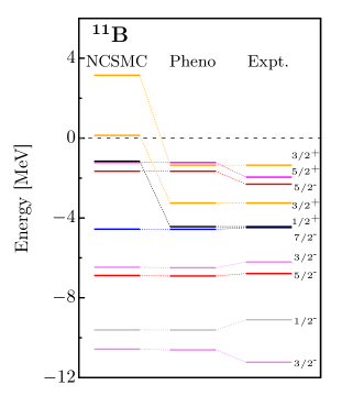
We start by performing NCSM calculations for ^10,11Be and ¹¹B. The obtained eigenvalues and eigenvectors serve as input for the NCSMC. For the expansion in Eq. (3), we used the ¹⁰Be $0^{+}$ ground state and the first excited $2^{+}$ state, the lowest 12 (10) positive (negative) parity eigenstates for ¹¹Be, and 20 (12) positive (negative) eigenstates for ¹¹B with $J$ ranging from $1/2$ to $11/2$. The resulting NCSMC energy spectra of ¹¹Be and ¹¹B are shown in Figs. 1 and 2, respectively. We present only states corresponding to experimentally bound states with respect to the ¹⁰Be$+$p (for ¹¹B) and ¹⁰Be$+$n (for ¹¹Be) threshold.

Figure 1: Calculated and experimental levels of ¹¹Be. Only states corresponding to experimentally bound states with respect to the ¹⁰Be$+$n threshold (horizontal red dashed line) are shown. The left column shows the original ab initio NCSMC calculation in $N_{\rm max}{=}7$ space. The phenomenological adjusted calculation is presented in the middle column. See the text for details.

Figure 2: Calculated and experimental levels in ¹¹B. Selected states corresponding to experimentally bound states with respect to the ¹⁰Be$+$p threshold (horizontal red dashed line) are shown. The SRG evolved $NN$-N⁴LO(500)$+3N_{\rm lnl}$ interaction was used. The left column shows the original ab initio NCSMC calculation in $N_{\rm max}{=}7$ space. The phenomenolgically adjusted calculation is presented in the middle column. See the text for details. The isospin of all shown states is $T{=}1/2$.

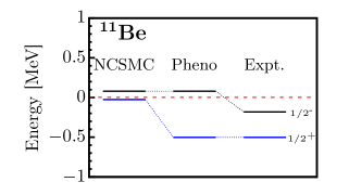
The low-lying level ordering in ¹¹Be is important because the energies of the $1/2^{+}$ and $1/2^{-}$ states are inverted compared to what would be expected from a standard shell-model picture. Our chosen interaction reproduces this parity inversion in the resulting NCSMC levels, as can be seen in Fig. 1. In previous NCSMC calculations using different interactions, the parity inversion could be reproduced with the non-local N²LO_sat interaction [27] but not using interactions with local $3N$ [28]. Since the $NN$-N⁴LO(500)$+3N_{\rm lnl}$ interaction reproduces this peculiarity of ¹¹Be, we feel that (i) the non-locality of the $3N$ interaction is an important feature for the description of exotic nuclei (i.e. it leads to a better reproduction of the extended nuclear density) and (ii) the selected interaction is appropriate for calculating the ¹¹Be $\beta$ decay. The present description is still showing discrepancies with data as the $1/2^{+}$ state is less bound than in experiment and the experimentally very weakly bound $1/2^{-}$ state is obtained just above the ¹⁰Be$+$n threshold.

The lowest negative-parity ¹¹B levels are well reproduced in our calculations with an under-prediction of the splitting between the $3/2^{-}$ ground state and the $1/2^{-}$ first excited state, indicating a weaker spin-orbit strength of the employed interaction. The lowest $5/2^{-}$ and $7/2^{-}$ as well as $3/2^{-}_{2}$ and $5/2^{-}_{2}$ states match well the experimental energies. The experimental $3/2^{-}_{3}$ state at 8.56 MeV (not shown in Fig. 2) with a pronounced $\alpha$-cluster structure is, however, overpredicted in the present NCSMC calculations [29]. Similarly, the lowest positive parity states appear more than 2.5 MeV too high. This is in part a consequence of the missing ⁷Li${+}\alpha$ mass partition in the calculations that we were not able to include for technical reasons. The ⁷Li${+}\alpha$ threshold appears experimentally 2.56 MeV below the ¹⁰Be$+$p threshold. The focus of this work is in particular on the $T{=}1/2$ $1/2^{+}$ and $3/2^{+}$ states in ¹¹B. As seen in Fig. 2, we obtain one $T{=}1/2$ $1/2^{+}$ bound state and the lowest $3/2^{+}$ state is just above the ¹⁰Be$+$p threshold.

Figure 3: NCSMC-calculated ¹⁰Be$+$p diagonal phase shifts. The solid lines correspond to the ${}^{2}S_{1/2}$ (or ${}^{2}P_{1/2}$) channels while the dashed and dotted curves correspond to the ${}^{4}D_{1/2}$ and ${}^{6}D_{1/2}$ channels, respectively. The vertical dashed line indicates the experimentally-predicted location of the $(1/2^{+},1/2)$ resonance at 197 keV. (a) NCSMC-calculated phase shifts using $N_{\rm max}{=}5$ basis size. (b) NCSMC-calculated phase shifts using $N_{\rm max}{=}7$ basis size. (c) Phenomenologically adjusted, NCSMC_pheno, phase shifts such that the $(1/2^{+},1/2)$ resonance coincides with the experimentally-predicted resonance at 197 keV. The $(3/2^{+},1/2)$ resonance is the result of shifting the degenerate states to the corresponding experimental levels (see Fig. 2). See the text for details. $E_{\rm c.m.}$ is the kinetic energy of ¹⁰Be$+$p in the center-of-mass frame.

Figure 4: NCSMC-calculated ¹⁰Be$+$p eigenphase shifts. The vertical dashed line indicates the experimentally-predicted location of the $(1/2^{+},1/2)$ resonance at 197 keV. (a) NCSMC-calculated phase shifts using $N_{\mathrm{max}}=5$ basis size. (b) NCSMC-calculated phase shifts using $N_{\rm max}{=}7$ basis size. The solid lines correspond to the first while the dashed and dotted curves correspond to the second and the third eigenphase shift, respectively. The sharp resonance in the $(1/2^{+},1/2)$ solid line in (b) is not shifted by $\pi$ for clarity. $E_{\rm c.m.}$ is the kinetic energy of ¹⁰Be$+$p in the center-of-mass frame.

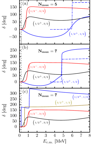
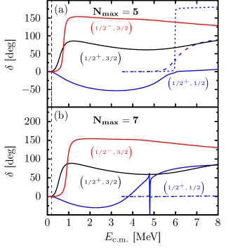
In addition to bound-state energy spectra, the NCSMC provides the low-energy phase shifts and eigenphase shifts for the ¹⁰Be$+$p channel, see Figs. 3 and 4, respectively. To show the effect of increasing the basis size, both the $N_{\rm max}{=}5$ and $N_{\rm max}{=}7$ results are presented in Fig. 3(a) and Fig. 3(b), respectively, and similarly for the eigenphase shifts in Fig. 4. The $(1/2^{-},3/2)$ and $(1/2^{+},3/2)$ phase shifts, isobaric analogues of the two bound states in ¹¹Be, are plotted to emphasize the parity inversion discussed in the previous paragraph. Both the $N_{\rm max}{=}5$ and $N_{\rm max}{=}7$ calculations reproduce the parity inversion in that the $(1/2^{+},3/2)$ resonance is lower in energy than the $(1/2^{-},3/2)$ resonance. The separation between these two resonances is more pronounced in the more converged result of $N_{\rm max}{=}7$ (see Fig. 3(b)).

$J^{\pi}$	$S(^{11}$B$\rightarrow^{10}$Be$)$	$S(^{11}$B$\rightarrow^{10}$B$)$		$S(^{11}$B$\rightarrow^{7}$Li$)$
	$(0^{+},1)$	$(1_{1}^{+},0)$	$(1_{2}^{+},0)$	$(3/2^{+},1/2)$
$1/2_{1}^{+}$	0.276	0.250	$2\times 10^{-4}$	0.218
$1/2_{2}^{+}$	0.0525	0.171	0.562	0.002
$1/2_{3}^{+}$	0.067	0.231	0.188	0.011
$3/2_{1}^{+}$	0.079	$6\times 10^{-4}$	0.215	0.009
$3/2_{2}^{+}$	$4\times 10^{-4}$	0.581	0.002	0.012
$3/2_{3}^{+}$	$6\times 10^{-4}$	0.011	0.006	0.021
$3/2_{4}^{+}$	0.067	0.034	0.35	0.006

Table 1: NCSM spectroscopic factors calculated from the overlap between select ¹¹B states and ¹⁰Be, ¹⁰B, and ⁷Li states. The first column displays the $J^{\pi}$ of each considered $T=1/2$ ¹¹B state. Spectroscopic factors of the ground states of ¹⁰B and ¹⁰Be and the first two $(1^{+},0)$ excited states of ¹⁰B are presented.

Shifting focus to the $(1/2^{+},1/2)$ phase shifts, two resonances are present - one broad and one sharp. Thus, the NCSMC supports the existence of a $(1/2^{+},1/2)$ resonance in the ¹⁰Be$+$p system. However, the energy of either resonance is higher than the experimental prediction of 197 keV. Furthermore, it is unclear which resonance should correspond to the experimental prediction. To gain insight in the structure of the $1/2^{+}$ states, we follow Ref. [30] to calculate the overlap between the corresponding NCSM ¹¹B states and the ¹⁰Be ground state, ¹⁰B $(1^{+},0)$ excited states, and the ⁷Li ground state (see Table 1). The first $1/2^{+}$ state with the largest overlap with the ¹⁰Be ground state corresponds to the bound state shown in Fig. 2 while the second and third $1/2^{+}$ states, corresponding to the two $(1/2^{+},1/2)$ resonances in Fig. 3, have comparably low overlaps. While these proton spectroscopic factors do not distinguish between the two resonances, the large $1/2^{+}_{2}$ ¹⁰B overlap indicates that its corresponding NCSMC resonance contains significant single-neutron content. From this, it is clear that the sharp resonance is caused by the lack of ¹⁰B $1^{+}$ channels and would be broadened by their inclusion in the NCSMC calculation. With the sharp resonance classified, the broad resonance must therefore correspond to the $1/2_{3}^{+}$ NCSM state and be the candidate for the experimentally-measured proton resonance.

III.2 Phenomenologically adjusted NCSMC

With the resonance identified, the next step is to calculate the branching ratio for the $\beta$-decay from the ¹¹Be ground state to the ¹¹B proton resonance. In order to better evaluate how well this resonance explains the experimentally observed branching ratio, we introduce a phenomenological shift to the NCSMC calculation (see, e.g., Ref. [28]) resulting in the calculated resonance lying at 197 keV, see Fig. 3(c). This approach, dubbed NCSMC_pheno, proceeds by using the ¹⁰Be, ¹¹B, and ¹¹Be NCSM eigenenergies as adjustable parameters in the NCSMC equations. First, the ¹⁰Be $2^{+}$ excitation energy is set to its experimental value (a change from NCSM calculated 3.48 MeV to experimental 3.37 MeV). We then adjust only the $1/2^{+}$ and $3/2^{+}$ channels relevant for the $\beta$ decay calculations. Consequently, there is almost no change in energies of negative parity states and the $5/2^{+}$ state in Figs. 1 and 2, and in the $T{=}3/2$ phase shift in Fig. 3(c). The fact that the $(1/2^{+},1/2)$ resonances shift slightly more than 1 MeV lower in energy when increasing the basis size from $N_{\rm max}{=}5$ to the $N_{\rm max}{=}7$ (compare Figs. 3(a), 4(a) and  3(b), 4(b)) implies that a larger model space can bring the resonance down further. Thus, this phenomenological shift is emulating the effect of including more channels. In addition to shifting the $(1/2^{+},1/2)$ resonance to 197 keV, we shift the ¹¹B $(3/2^{+},1/2)$ levels as well as the ¹¹Be ground state to its experimental value, see Figs. 1 and 2. These phenomenological shifts bring the NCSMC major shell splittings closer to experimental values. A consequence of shifting the first two $(3/2^{+},1/2)$ ¹¹B levels is the emergence of a sharp resonance (previously broad and higher in energy) just 573 keV above threshold in Fig. 3. The location of this resonance is similar to the predicted resonance at 262 keV in Ref. [31]. The authors of Ref. [31] suggest that this could be the unassigned resonance observed in Ref. [32].

III.3 ¹¹Be $\beta$ decay

We first calculate $B(\mathrm{GT})$ for the $\beta$-decay from the ¹¹Be ground state to the first bound $(1/2^{+},1/2)$ state in ¹¹B. This level is shifted to its experimental value as well, see Fig. 2. The results are shown in Table 2. Also shown in Table 2 is the $B(\mathrm{GT})$ calculated for the $\beta$-decay to the three bound $(3/2^{+},1/2)$ states. The third bound $(3/2^{+},1/2)$ state is a result of phenomenologically shifting the first two levels to their corresponding experimental values. To determine the half-life from $B(\mathrm{GT})$, we use [1]:

$$fT^{p}_{1/2}=\frac{6141}{g_{A}^{2}B(\mathrm{GT})},$$ (6)

where $g_{A}{=}-1.27$ is the GT coupling constant, $f$ is a phase-space factor determined by the $Q$-value of the decay, and $T^{p}_{1/2}$ is the half-life of the decay. The half-life of the decay can be used to calculate the corresponding branching ratio using the following expression:

$$b_{p}=\frac{T^{{}^{11}{\rm Be}}_{1/2}}{T^{p}_{1/2}},$$ (7)

where $T^{{}^{11}{\rm Be}}_{1/2}=13.8\;s$ is the half-life of the ¹¹Be nucleus. Using Eqs. (6) and (7), the experimental branching ratios (see Ref. [4]) were converted to the $B(\mathrm{GT})$ values in Table 2. It is clear from Table. 2 that the inclusion of the proton and neutron channels in the NCSMC improves the calculated $B(\mathrm{GT})$ values over the NCSM results.

$B(\mathrm{GT})$	NCSM	NCSMCpheno	Expt.
$1/2^{+}_{1}$	0.341	0.277	0.004
$3/2^{+}_{1}$	0.023	0.002	0.010
$3/2^{+}_{2}$	2.92	0.286	0.228
$3/2^{+}_{3}$	0.011	$7\times 10^{-5}$	-

Table 2: $B(\mathrm{GT})$ values from the ground state of ¹¹Be to the specified bound states of ¹¹B. The first column displays the $J^{\pi}$ of each considered $T=1/2$ ¹¹B state. The NCSMC_pheno approach was applied. Both the NCSM and NCSMC_pheno values were obtained at $N_{\mathrm{max}}=7$. Experimental values obtained as branching ratios from Ref. [4] and converted to $B(\mathrm{GT})$ values (see text).

The transition strength to the $1/2_{1}^{+}$ state is unexpectedly large compared to the experimental strength. This is indicative of the mixing of strength between the bound $1/2_{1}^{+}$ state and the resonance in question. It is also worth noting that the overlap between the $1/2_{1}^{+}$ state and both the ⁷Li$+\alpha$ ground and ¹⁰B$+$n $(1_{1}^{+},0)$ states is significant (see Table 1). Thus, the inclusion of these channels in the NCSMC calculation could address this discrepancy. The NCSMC_pheno calculations of the experimentally strong transition to the $3/2^{+}_{2}$ state show great improvement over the NCSM calculations. The cause of the enhanced NCSM $B(\mathrm{GT})$ value can be attributed to the large overlap with the ¹⁰B$+$n $(1_{1},0)$ state (see Table. 1). With the inclusion of the ¹⁰Be+$n$ channel in the NCSMC calculation, the halo structure of ¹¹Be is reproduced which has a small overlap with the ¹¹B $3/2^{+}_{2}$ state thus suppressing the NCSMC $B(\mathrm{GT})$.

Figure 5: Energy-dependent $B_{\mathrm{GT}}(E)$ calculated from the ground state of ¹¹Be to the $(1/2^{+},1/2)$ proton continuum of ¹¹B using the NCSMC.

The calculation of the branching ratio for the $\beta$-decay to the $(1/2^{+},1/2)$ resonance is more involved since the final state in Eq. (1) is an energy-dependent scattering wave function. The scattering wave function is calculated in $k$-space (using the same same convention from Ref. [13]), thus the matrix element in Eq. (1) must be evaluated with a volume integral in $k$-space,

$$B(\mathrm{GT})=4\pi\int_{k_{min}}^{k_{max}}dkk^{2}B_{\mathrm{GT}}(k),$$ (8)

where $k_{min}$ and $k_{max}$ are chosen to isolate the location of the resonance. In order to calculate the branching ratio for this process, $B_{\mathrm{GT}}(k)$ must be folded with the energy-dependent phase-space factor $f$. Thus, we first transform Eq. (8) to energy-space such that

$$B(GT)=\int_{E_{min}}^{E_{max}}dEB_{\mathrm{GT}}(E),$$ (9)

where

$$B_{\mathrm{GT}}(E):=\frac{4\pi\mu k}{\hbar^{2}}B_{\mathrm{GT}}(k)$$ (10)

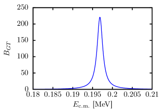
and $k=\frac{\sqrt{2\mu E}}{\hbar}$ with $\mu$ the reduced mass. The energy-dependent $B_{\mathrm{GT}}(E)$ is shown in Fig. 5, where it displays a prominent peak at the resonance energy of 197 keV. The sharp peak in $B_{\mathrm{GT}}(E)$ is a visual representation of how a resonance can enhance the $\beta$-decay transition rate to the continuum. The $Q$-value at a given energy can be expressed as $Q=Q_{0}-E$ where $Q_{0}=0.281$ MeV is the Q-value evaluated at the p${+}^{10}$Be threshold. The branching ratio of the $\beta$-decay to the resonance can be calculated by combining Eqs. (6), (7), and (9) in the following way:

$$b_{p}=\frac{T_{1/2}^{{}^{11}{\rm Be}}g_{A}^{2}}{6141}\int_{E_{min}}^{E_{max}}dEB_{\mathrm{GT}}(E)f(Q_{0}-E).$$ (11)

$(1/2^{+},1/2)$	$N_{\rm max}=5$		$N_{\rm max}=7$		Expt.
	NCSM	NCSMCpheno	NCSM	NCSMCpheno
$B(\mathrm{GT})$	1.95	0.325	1.39	0.565	$5.5^{8.3}_{3.3}$
$b_{p}$	-	$7.4\times 10^{-7}$	-	$1.3\times 10^{-6}$	$1.3(3)\times 10^{-5}$

Table 3: $B(\mathrm{GT})$ $\beta$-decay values for the transition from the ground state of ¹¹Be to the p+¹⁰Be resonance. The NCSM results correspond to the $(1/2_{3}^{+},1/2)$ state. The experimental values are those presented in Ref. [6]

Using Eq. (11), we integrate $B_{\mathrm{GT}}(E)$ over the energy-range shown in Fig. 5 resulting in the values shown in Table 3. The NCSMC $B(\mathrm{GT})$ value reported in Table 3 is calculated as $B(\mathrm{GT})=\int dEB_{\mathrm{GT}}(E)$. Although the calculated branching ratio, $b_{p}=(1.3\pm 0.5)\times 10^{-6}$, is lower than the two experimental observations [5, 6], it is consistent when taking into account that the non-resonant decay branching ratio calculated in Ref. [2] is two orders of magnitude smaller. The uncertainty is estimated by comparing the NCSMC_pheno results using $N_{\rm max}=5$ and $N_{\rm max}=7$. To verify that we shifted the correct resonance, we also calculated $B(\mathrm{GT})=0.0483$ for the transition to the $(1/2^{+},1/2)$ resonance located around $1$ MeV in Fig. 3(c). This weak transition strength confirms that we have chosen the correct candidate. We also investigate the sharp $(3/2^{+},1/2)$ resonance in Fig. 3(c) as it was suggested as a candidate for the large branching ratio [6]. While there is a non-negligible overlap between $3/2^{+}_{4}$ and ¹⁰Be+p (see Table 1), we calculate that $B(\mathrm{GT})=0.00131$ for this particular resonance. This is contrary to the large $B(\mathrm{GT})$ empirically calculated for this resonance in Ref [31]. It is also worth nothing that the $\alpha$ spectroscopic factors for the $1/2_{2}$ and $1/2_{3}$ states in Table 1 are significantly smaller than those calculated in the shell model calculations in Ref. [3]. The smaller spectroscopic factors indicate that the proton decay channel will not have as much competition with the $\alpha$ decay channel as was indicated of Ref. [3]. With these considerations, we conclude that the large observed branching is due to the existence of this $(1/2^{+},1/2)$ p+¹⁰Be resonance.

IV Conclusions

Using the ab initio NCSMC, we investigated the bound energy-levels and low-lying resonances in both ¹¹Be and ¹¹B. The two- and three-body interactions, $NN$-N⁴LO(500)$+3N_{\rm lnl}$, produce realistic energy spectra in both ¹¹Be and ¹¹B. The experimentally-observed parity inversion in ¹¹Be is reproduced. We identified two $(1/2^{+},1/2)$ resonances in the p+¹⁰Be continuum and determined that the broad resonance dominated by the $1/2^{+}_{3}$ NCSM state is the candidate resonance. The location of the resonance is several MeV higher than the experimentally predicted location of 197 keV although its position decreases dramatically with the increasing basis size. In order to determine if this resonance can explain the large branching ratio observed by experiment, we phenomenologically shifted the NCSMC resonance to 197 keV.

With the resonance determined, we developed the procedure to calculate $B(\mathrm{GT})$ fully within the NCSMC. Appendix A contains the relevant derivations. We then extended the calculation to the continuum by deriving the necessary expressions to calculate the branching ratio for the decay to a resonance state (in the p+¹⁰Be continuum). The resulting branching ratio for the $\beta$-decay to the candidate $(1/2^{+},1/2)$ resonance is $b_{p}=(1.3\pm 0.5)\times 10^{-6}$. This calculated branching ratio is consistent with both experimental branching ratios reported Ref. [5] and Ref. [6] taking into account that the non-resonant decay branching ratio is two orders of magnitude smaller. Furthermore, we calculate a small $B(\mathrm{GT})$ for the nearby $(3/2^{+},1/2)$ resonance which further reinforces our conclusions.

The present calculations can be further improved by including the ⁷Li+$\alpha$ and ¹⁰B+n mass partitions. The former would particularly impact the description of the $1/2^{+}_{1}$ bound state and presumably redistribute some of the $B(\mathrm{GT})$ strength from the bound state to the $(1/2^{+},1/2)$ resonance. Work in this direction is under way, see Ref. [33] for the latest developments regarding the inclusion of $\alpha$ clustering in the NCSMC.

V Acknowledgements

This work was supported by the NSERC Grant No. SAPIN-2016-00033 and by the U.S. Department of Energy, Office of Science, Office of Nuclear Physics, under Work Proposals No. SCW0498. TRIUMF receives federal funding via a contribution agreement with the National Research Council of Canada. This work was prepared in part by LLNL under Contract No. DE-AC52-07NA27344. Computing support came from an INCITE Award on the Summit supercomputer of the Oak Ridge Leadership Computing Facility (OLCF) at ORNL, from Livermore Computing, Westgrid and Compute Canada.

Appendix A Derivation of $B(\mathrm{GT})$ in the NCSMC

To calculate $B(\mathrm{GT})$, the reduced matrix element of the GT operator is calculated with NCSMC initial and final states. We derive this reduced matrix element for a general coordinate-independent one-body operator, $\mathcal{O}^{(\kappa\tau)}_{\mu_{\tau}}$ with $\kappa$ and $\tau$ the spin and isospin rank, respectively, and $\mu_{\tau}$ the isospin projection, e.g., GT, Fermi, spin part of the M1 operator. The GT operator corresponds to the case where $\kappa{=}1$, $\tau{=}1$, and $\mu_{\tau}{=}+1$. Inserting the form of the NCSMC wave function (Eqs.(3) and (4)) in Eq. (1) leads to four contributions:

$$\Braket{\Psi^{J_{f}^{\pi_{f}}T_{f}}_{f\;\;M_{T_{f}}}}{\hat{\mathcal{O}}^{(\kappa\tau)}_{\mu_{\tau}}}{\Psi^{J_{i}^{\pi_{i}}T_{i}}_{i\;\;M_{T_{i}}}}=$$

$$\sum_{\lambda_{i}\lambda_{f}}\tilde{c}^{*}_{\lambda_{f}}\tilde{c}_{\lambda_{i}}\Braket{A\lambda_{f}J_{f}T_{f}M_{T_{f}}}{\hat{\mathcal{O}}^{(\kappa\tau)}_{\mu_{\tau}}}{A\lambda_{i}J_{i}T_{i}M_{T_{i}}}$$

$$+\sum_{\lambda_{f}\nu_{i}}\tilde{c}^{*}_{\lambda_{f}}\int_{0}^{\infty}drr^{2}\tilde{\chi}_{\nu_{i}}(r)\textstyle{\frac{1}{r}}$$

$$\times\Braket{A\lambda_{f}J_{f}T_{f}M_{T_{f}}}{\hat{\mathcal{O}}^{(\kappa\tau)}_{\mu_{\tau}}\hat{\mathcal{A}}_{\nu_{i}}}{\Phi_{\nu_{i}r}^{J_{i}T_{i}M_{T_{i}}}}$$

$$+\sum_{\lambda_{i}\nu_{f}}\tilde{c}_{\lambda_{i}}\int_{0}^{\infty}drr^{2}\tilde{\chi}^{*}_{\nu_{f}}(r)\textstyle{\frac{1}{r}}$$

$$\times\Braket{\Phi_{\nu_{f}r}^{J_{f}T_{f}M_{T_{f}}}}{\hat{\mathcal{A}}_{\nu_{f}}\hat{\mathcal{O}}^{(\kappa\tau)}_{\mu_{\tau}}}{A\lambda_{i}J_{i}T_{i}M_{T_{i}}}$$

$$+\sum_{\nu_{f}\nu_{i}}\int_{0}^{\infty}dr^{\prime}r^{\prime 2}\tilde{\chi}^{*}_{\nu_{f}}(r^{\prime})\textstyle{\frac{1}{r^{\prime}}}\int_{0}^{\infty}drr^{2}\tilde{\chi}_{\nu_{i}}(r)\textstyle{\frac{1}{r}}$$

$$\times\Braket{\Phi_{\nu_{f}r^{\prime}}^{J_{f}T_{f}M_{T_{f}}}}{\hat{\mathcal{A}}_{\nu_{f}}\hat{\mathcal{O}}^{(\kappa\tau)}_{\mu_{\tau}}\hat{\mathcal{A}}_{\nu_{i}}}{\Phi_{\nu_{i}r}^{J_{i}T_{i}M_{T_{i}}}}\;.$$ (12)

The expansion coefficients $\tilde{c}$ and $\tilde{\chi}(r)$ can be related to the expansion (3) and NCSMC norm kernels according to Eqs. (20), (32) and (33) in Ref. [11]. We note that the $J^{\pi}TM_{T}$ quantum number dependence of these coefficients is not displayed to simplify the notation. Similarly, we omit the parity quantum number in most of the states. In the present case, $A{=}11$. We also note that matrix element (12) is reduced only in spin-space, not isospin-space.

In order to proceed with the derivation, all contributions from localized terms are calculated in a HO basis and then converted to coordinate space with the following relation [34]:

$$\Ket{\Phi_{\nu r}^{JTM_{T}}}=\sum_{n}\Ket{\Phi_{\nu n}^{JTM_{T}}}R_{n\ell}(r),$$ (13)

where $R_{nl}(r)$ are radial HO functions and

$$\ket{\Phi^{JTM_{T}}_{\nu n}}= \Big{[}\big{(}\ket{{}^{10}{\rm Be}\,\alpha_{1}I_{1}^{\pi_{1}}T_{1}}\ket{N\,\tfrac{1}{2}^{\texttt{+}}\tfrac{1}{2}}\big{)}^{(sT)}$$

$$\times\,Y_{\ell}(\hat{r}_{10,1})\Big{]}^{(J^{\pi}T)}_{M_{T}}\,R_{n\ell}(r_{10,1})\;,$$ (14)

with $N$ representing p for ¹¹B and n for ¹¹Be. See also the discussion in Sect. II.C.1 in Ref. [34].

The process to calculate each of the terms in Eq. (12) is analogous to the procedure for calculating the norm and Hamiltonian kernels for the NCSMC [13]. The first term in Eq. (12) involves NCSM matrix elements of $\hat{\mathcal{O}}^{(\kappa\tau)}_{\mu_{\tau}}$ calculated using standard second-quantization techniques. The second and third terms are analogous to the coupling kernels when solving the NCSMC Hamiltonian equations [13]. In order to continue, we represent the operator in a second-quantized form:

$$\hat{\mathcal{O}}^{(\kappa\tau)}_{\mu_{\kappa}\mu_{\tau}}=\left(\frac{-1}{\hat{\kappa}}\right)\sum\Braket{j_{a}\textstyle{\frac{1}{2}}m_{t_{a}}}{\hat{\mathcal{O}}^{(\kappa\tau)}_{\mu_{\tau}}}{j_{b}\textstyle{\frac{1}{2}}m_{t_{b}}}$$

$$\times\hat{a}^{\dagger}_{j_{a}m_{a}\textstyle{\frac{1}{2}}m_{t_{a}}}\tilde{a}_{j_{b}m_{b}\textstyle{\frac{1}{2}}m_{t_{b}}}\Braket{j_{a}m_{a}j_{b}m_{b}}{\kappa\mu_{\kappa}}\;,$$ (15)

with $\tilde{a}_{jm\textstyle{\frac{1}{2}}m_{t}}{=}(-1)^{j-m}a_{j\;-m\;\textstyle{\frac{1}{2}}m_{t}}$. To expand this term, we also represent the cluster wave function in a second-quantized form (see Sect. II.D.2 of Ref. [34] and Sect. II.A of Ref. [35]):

$$\hat{\mathcal{A}}_{\nu} \ket{\Phi_{\nu n}^{J_{i}M_{i}T_{i}M_{T_{i}}}}_{\rm SD}=\sum(-1)^{I_{1}+J_{i}+j}\hat{s}\hat{j}\begin{Bmatrix}I_{1}&\textstyle{\frac{1}{2}}&s\\ \ell&J_{i}&j\end{Bmatrix}$$

$$\times\Braket{I_{1}M_{1}jm}{J_{i}M_{i}}\Braket{T_{1}M_{T_{1}}\textstyle{\frac{1}{2}}m_{t}}{T_{i}M_{T_{i}}}$$

$$\times\hat{a}^{\dagger}_{n\ell jm\textstyle{\frac{1}{2}}m_{t}}\ket{{}^{10}{\rm Be}\,\alpha_{1}I_{1}M_{1}T_{1}M_{T_{1}}}_{\rm SD},$$ (16)

where $\ket{{}^{10}{\rm Be}\,\alpha_{1}I_{1}M_{1}T_{1}M_{T_{1}}}_{\rm SD}$ is an NCSM state of the $(A{-}1)$ system ¹⁰Be expanded in the HO Slater Determinant (SD) basis, $\begin{Bmatrix}I_{1}&I_{2}&s\\ \ell&J_{i}&j\end{Bmatrix}$ is the standard Wigner 6j-symbol [36], and $\hat{x}$ denotes $\sqrt{2x+1}$. The $nl$ HO quantum numbers in the $nlj$ single-particle states are omitted from now on for simplicity. The relationship between the SD eigenstates entering Eq. (16) and the relative coordinate eigenstates in Eqs. (4) and (14) is given by

$$\ket{{}^{10}{\rm Be}\,\alpha_{1}I_{1}M_{1}T_{1}M_{T_{1}}}_{\rm SD} =\ket{{}^{10}{\rm Be}\,\alpha_{1}I_{1}M_{1}T_{1}M_{T_{1}}}$$

$$\times\,\varphi_{00}(\vec{R}^{(10)}_{\rm c.m.})\;,$$ (17)

with $\vec{R}^{(10)}_{\rm c.m.}$ the c.m. coordinate of ¹⁰Be and $\varphi_{00}$ the HO wave function of the c.m. motion. Using Eq. (16), the coupling term becomes:

$${}_{\rm SD}\Braket{A\lambda J_{f}T_{f}M_{T_{f}}}{\hat{\mathcal{O}}^{(\kappa\tau)}_{\mu_{\tau}}\hat{\mathcal{A}}_{\nu}}{\Phi_{\nu n}^{J_{i}T_{i}M_{T_{i}}}}_{\rm SD}=\sum(-1)^{1+\kappa+J_{f}-J_{i}}\hat{J}_{i}\hat{s}\hat{j}\begin{Bmatrix}I_{1}&j&J_{i}\\ \kappa&J_{f}&j_{a}\end{Bmatrix}\begin{Bmatrix}I_{1}&\textstyle{\frac{1}{2}}&s\\ \ell&J_{i}&j\end{Bmatrix}\Braket{T_{1}M_{T_{1}}\textstyle{\frac{1}{2}}m_{t}}{T_{i}M_{T_{i}}}$$

$$\times\Braket{j_{a}\textstyle{\frac{1}{2}}m_{t_{a}}}{\hat{\mathcal{O}}^{(\kappa\tau)}_{\mu_{\tau}}}{j\textstyle{\frac{1}{2}}m_{t}}\,_{\rm SD}\Braket{A\lambda J_{f}T_{f}M_{T_{f}}}{\hat{a}^{\dagger}_{j_{a}\textstyle{\frac{1}{2}}m_{t_{a}}}}{A{-}1\,\alpha_{1}I_{1}T_{1}M_{T_{1}}}_{\rm SD}$$

$$+\sum(-1)^{J_{f}-J_{1}+J_{2}+j_{b}+\kappa-J_{i}}\hat{s}\hat{j}\hat{J}_{i}\hat{J}_{1}\hat{J}_{2}\begin{Bmatrix}j_{a}&j_{b}&\kappa\\ J_{1}&j&J_{2}\end{Bmatrix}\begin{Bmatrix}I_{1}&j&J_{i}\\ \kappa&J_{f}&J_{1}\end{Bmatrix}\begin{Bmatrix}I_{1}&\textstyle{\frac{1}{2}}&s\\ \ell&J_{i}&j\end{Bmatrix}\Braket{T_{1}M_{T_{1}}\textstyle{\frac{1}{2}}m_{t}}{T_{i}M_{T_{i}}}$$

$$\times\Braket{j_{a}\textstyle{\frac{1}{2}}m_{t_{a}}}{\hat{\mathcal{O}}^{(\kappa\tau)}_{\mu_{\tau}}}{j_{b}\textstyle{\frac{1}{2}}m_{t_{b}}}\,_{\rm SD}\Braket{A\lambda J_{f}T_{f}M_{T_{f}}}{\left[(\hat{a}^{\dagger}_{j_{a}\textstyle{\frac{1}{2}}m_{t_{a}}}\hat{a}^{\dagger}_{j\textstyle{\frac{1}{2}}m_{t}})^{(J_{2})}\tilde{a}_{j_{b}\textstyle{\frac{1}{2}}m_{t_{b}}}\right]^{(J_{1})}}{A{-}1\,\alpha_{1}I_{1}T_{1}M_{T_{1}}}_{\rm SD},$$ (18)

where $\Braket{\hat{a}^{\dagger}_{j_{a}\textstyle{\frac{1}{2}}m_{t_{a}}}}$ and $\Braket{\left[\left(\hat{a}^{\dagger}_{j_{a}\textstyle{\frac{1}{2}}m_{t_{a}}}\hat{a}^{\dagger}_{j\textstyle{\frac{1}{2}}m_{t}}\right)^{(J_{2})}\tilde{a}_{j_{b}\textstyle{\frac{1}{2}}m_{t_{b}}}\right]^{(J_{1})}}$ are 1-particle and 2-particle-1-hole transition matrices between the composite and the target (here ¹¹B and ¹⁰Be) NCSM wave functions. Similarly as for the target eigenstates (17), the composite system (¹¹Be or ¹¹B) eigenstates expanded in the HO SD basis are related to the relative coordinate eigenstates appearing in Eq. (12) by

$$\Ket{A\lambda JTM_{T}}_{\rm SD}=\Ket{A\lambda JTM_{T}}\varphi_{00}(\vec{\xi}_{0})\;,$$ (19)

with $\vec{\xi}_{0}$ the c.m. coordinate of the composite $A$-nucleon system and $\varphi_{00}$ the HO wave function of the c.m. motion. See also the appendix of Ref. [11] and Ref. [35]. The third term in Eq. (12) is calculated by taking advantage of the following relation:

$${}_{\rm SD}\Braket{A\lambda_{f}J_{f}T_{f}M_{T_{f}}}{\hat{\mathcal{O}}^{(\kappa\tau)}_{\mu_{\tau}}\hat{\mathcal{A}}_{\nu}}{\Phi_{\nu n}^{J_{i}T_{i}M_{T_{i}}}}_{\rm SD}=(-1)^{J_{f}-J_{i}}\,\;_{\rm SD}\Braket{\Phi_{\nu n}^{J_{i}T_{i}M_{T_{i}}}}{\left[\hat{\mathcal{O}}^{(\kappa\tau)}_{\mu_{\tau}}\hat{\mathcal{A}}_{\nu}\right]^{\dagger}}{A\lambda_{f}J_{f}T_{f}M_{T_{f}}}_{\rm SD}.$$ (20)

Thus, Eq. (18) is sufficient for both coupling terms in Eq. (12).

The last term in Eq. (12) is derived using a similar procedure:

$${}_{\rm SD}\Braket{\Phi_{\nu^{\prime}n^{\prime}}^{J_{f}T_{f}M_{T_{f}}}}{\hat{A}_{\nu^{\prime}}\hat{\mathcal{O}}^{(\kappa\tau)}_{\mu_{\tau}}\hat{A}_{\nu}}{\Phi_{\nu n}^{J_{i}T_{i}M_{T_{i}}}}_{\rm SD}=\delta_{\alpha_{1}\alpha_{1}^{\prime}}\delta_{I_{1}I_{1}^{\prime}}\delta_{T_{1}T_{1}^{\prime}}\delta_{M_{T_{1}}M^{\prime}_{T_{1}}}\hat{J_{f}}\hat{J_{i}}\hat{s}\hat{s}^{\prime}$$

$$\times\sum\hat{j}\hat{j}^{\prime}(-1)^{I_{1}+\kappa+J_{i}+j^{\prime}}\begin{Bmatrix}I_{1}&j&J_{i}\\ \kappa&J_{f}&j^{\prime}\\ \end{Bmatrix}\begin{Bmatrix}I_{1}&\textstyle{\frac{1}{2}}&s\\ \ell&J_{i}&j\\ \end{Bmatrix}\begin{Bmatrix}I_{1}&\textstyle{\frac{1}{2}}&s^{\prime}\\ \ell^{\prime}&J_{f}&j^{\prime}\\ \end{Bmatrix}$$

$$\times\Braket{j^{\prime}\textstyle{\frac{1}{2}}m_{t}^{\prime}}{\hat{\mathcal{O}}^{(\kappa\tau)}_{\mu_{\tau}}}{j\textstyle{\frac{1}{2}}m_{t}}\Braket{T_{1}M_{T_{1}}\textstyle{\frac{1}{2}}m_{t}}{T_{i}M_{T_{i}}}\Braket{T_{1}M_{T_{1}}\textstyle{\frac{1}{2}}m_{t}^{\prime}}{T_{f}M_{T_{f}}}$$

$$-\sum\hat{s}\hat{s}^{\prime}\hat{j}\hat{j^{\prime}}\hat{J_{f}}\hat{J_{i}}\hat{J_{2}}\hat{J_{3}}\hat{J_{4}}(-1)^{j^{\prime}+j_{a}+\kappa+J_{3}+j_{b}+I_{1}-J_{f}}\begin{Bmatrix}I_{1}&\frac{1}{2}&s\\ \ell&J_{i}&j\\ \end{Bmatrix}\begin{Bmatrix}I_{1}^{\prime}&\frac{1}{2}&s^{\prime}\\ \ell^{\prime}&J_{f}&j^{\prime}\\ \end{Bmatrix}\begin{Bmatrix}-&j&I_{1}&J_{i}\\ j^{\prime}&-&I_{1}^{\prime}&J_{f}\\ j_{b}&j_{a}&-&\kappa\\ J_{4}&J_{2}&J_{3}&-\end{Bmatrix}$$

$$\times_{\rm SD}\Braket{A{-}1\,\alpha_{1}^{\prime}I_{1}^{\prime}T_{1}^{\prime}M_{T_{1}}^{\prime}}{\left[\left(\hat{a}^{\dagger}_{j_{a}\textstyle{\frac{1}{2}}m_{t_{a}}}\hat{a}^{\dagger}_{j\textstyle{\frac{1}{2}}m_{t}}\right)^{(J_{2})}\left(\tilde{a}_{j^{\prime}\textstyle{\frac{1}{2}}m_{t}^{\prime}}\tilde{a}_{j_{b}\textstyle{\frac{1}{2}}m_{t_{b}}}\right)^{(J_{4})}\right]^{(J_{3})}}{A{-}1\,\alpha_{1}I_{1}T_{1}M_{T_{1}}}_{\rm SD}$$

$$\times\Braket{j_{a}\textstyle{\frac{1}{2}}m_{t_{a}}}{\hat{\mathcal{O}}^{(\kappa\tau)}_{\mu_{\tau}}}{j_{b}\textstyle{\frac{1}{2}}m_{t_{b}}}\Braket{T_{1}^{\prime}M_{T_{1}}^{\prime}\textstyle{\frac{1}{2}}m_{t}^{\prime}}{T_{f}M_{T_{f}}}\Braket{T_{1}M_{T_{1}}\textstyle{\frac{1}{2}}m_{t}}{T_{i}M_{T_{i}}}$$

$$-\sum\hat{s}\hat{s}^{\prime}\hat{j}\hat{j}^{\prime}\hat{J_{f}}\hat{J_{i}}\hat{J_{2}}(-1)^{j_{a}+j^{\prime}+I_{1}+I_{1}^{\prime}+\kappa+J_{i}+J_{f}}\begin{Bmatrix}I_{1}&\frac{1}{2}&s\\ \ell&J_{i}&j\\ \end{Bmatrix}\begin{Bmatrix}I_{1}^{\prime}&\frac{1}{2}&s^{\prime}\\ \ell^{\prime}&J_{f}&j^{\prime}\\ \end{Bmatrix}\begin{Bmatrix}j_{a}&j&\kappa\\ J_{i}&J_{f}&I_{1}\\ \end{Bmatrix}\begin{Bmatrix}I_{1}&j_{a}&J_{f}\\ j^{\prime}&I_{1}^{\prime}&J_{2}\\ \end{Bmatrix}$$

$$\times\Braket{j_{a}\textstyle{\frac{1}{2}}m_{t_{a}}}{\hat{\mathcal{O}}^{(\kappa\tau)}_{\mu_{\tau}}}{j\textstyle{\frac{1}{2}}m_{t}}_{\rm SD}\Braket{A{-}1\,\alpha_{1}^{\prime}I_{1}^{\prime}T_{1}^{\prime}M_{T_{1}}^{\prime}}{\left(\hat{a}^{\dagger}_{j_{a}\textstyle{\frac{1}{2}}m_{t_{a}}}\tilde{a}_{j^{\prime}\textstyle{\frac{1}{2}}m_{t}^{\prime}}\right)^{(J_{2})}}{A{-}1\,\alpha_{1}I_{1}T_{1}M_{T_{1}}}_{\rm SD}$$

$$\times\Braket{T_{1}M_{T_{1}}tm}{T_{i}M_{T_{i}}}\Braket{T_{1}^{\prime}M_{T_{1}}^{\prime}\textstyle{\frac{1}{2}}m_{t}^{\prime}}{T_{f}M_{T_{f}}}$$

$$-\sum\hat{j}\hat{j}^{\prime}\hat{s}\hat{s}^{\prime}\hat{J_{f}}\hat{J_{i}}\hat{J_{1}}(-1)^{j_{b}-j^{\prime}-\kappa+1}\begin{Bmatrix}I_{1}&\frac{1}{2}&s\\ \ell&J_{i}&j\\ \end{Bmatrix}\begin{Bmatrix}I_{1}^{\prime}&\frac{1}{2}&s^{\prime}\\ \ell^{\prime}&J_{f}&j^{\prime}\\ \end{Bmatrix}\begin{Bmatrix}I_{1}&j&J_{i}\\ j_{b}&I_{1}^{\prime}&J_{1}\\ \end{Bmatrix}\begin{Bmatrix}j^{\prime}&j_{b}&\kappa\\ J_{i}&J_{f}&I_{1}^{\prime}\\ \end{Bmatrix}$$

$$\times\Braket{j^{\prime}\textstyle{\frac{1}{2}}m_{t^{\prime}}}{\hat{\mathcal{O}}^{(\kappa\tau)}_{\mu_{\tau}}}{j_{b}\textstyle{\frac{1}{2}}m_{t_{b}}}_{\rm SD}\Braket{A{-}1\,\alpha_{1}^{\prime}I_{1}^{\prime}T_{1}^{\prime}M_{T_{1}}^{\prime}}{\left(\hat{a}^{\dagger}_{j\textstyle{\frac{1}{2}}m_{t}}\tilde{a}_{j_{b}\textstyle{\frac{1}{2}}m_{t_{b}}}\right)^{(J_{1})}}{A{-}1\,\alpha_{1}I_{1}T_{1}M_{T_{1}}}_{\rm SD}$$

$$\times\Braket{T_{1}M_{T_{1}}\textstyle{\frac{1}{2}}m_{t}}{T_{i}M_{T_{i}}}\Braket{T_{1}^{\prime}M_{T_{1}}^{\prime}\textstyle{\frac{1}{2}}m_{t}^{\prime}}{T_{f}M_{T_{f}}}$$

$$+\delta_{nn^{\prime}}\delta_{\ell\ell^{\prime}}\frac{\hat{s}\hat{s}^{\prime}\hat{J_{f}}\hat{J_{i}}}{\hat{\kappa}}(-1)^{I_{1}^{\prime}+l-{\textstyle\frac{1}{2}}+J_{i}+s+s^{\prime}}\begin{Bmatrix}s^{\prime}&s&\kappa\\ I_{1}&I_{1}^{\prime}&\textstyle{\frac{1}{2}}\\ \end{Bmatrix}\begin{Bmatrix}s^{\prime}&s&\kappa\\ J_{i}&J_{f}&\ell\\ \end{Bmatrix}\sum\Braket{j_{a}\textstyle{\frac{1}{2}}m_{t_{a}}}{\hat{\mathcal{O}}^{(\kappa\tau)}_{\mu_{\tau}}}{j_{b}\textstyle{\frac{1}{2}}m_{t_{b}}}$$

$$\times_{\rm SD}\Braket{A{-}1\,\alpha_{1}^{\prime}I_{1}^{\prime}T_{1}^{\prime}M_{T_{1}}^{\prime}}{\left[\hat{a}^{\dagger}_{j_{a}\textstyle{\frac{1}{2}}m_{t_{a}}}\tilde{a}_{j_{b}\textstyle{\frac{1}{2}}m_{t_{b}}}\right]^{(\kappa)}}{A{-}1\,\alpha_{1}I_{1}T_{1}M_{T_{1}}}_{\rm SD}$$

$$\times\Braket{T_{1}M_{T_{1}}\textstyle{\frac{1}{2}}m_{t}}{T_{i}M_{T_{i}}}\Braket{T_{1}^{\prime}M_{T_{1}}^{\prime}\textstyle{\frac{1}{2}}m_{t}}{T_{f}M_{T_{f}}}$$ (21)

where $\Braket{\left[\left(\hat{a}^{\dagger}_{j_{a}\textstyle{\frac{1}{2}}m_{t_{a}}}\hat{a}^{\dagger}_{j\textstyle{\frac{1}{2}}m_{t}}\right)^{(J_{2})}\left(\tilde{a}_{j^{\prime}\textstyle{\frac{1}{2}}m_{t}^{\prime}}\tilde{a}_{j_{b}\textstyle{\frac{1}{2}}m_{t_{b}}}\right)^{(J_{4})}\right]^{(J_{3})}}$, $\Braket{\left(\hat{a}^{\dagger}_{j_{a}\textstyle{\frac{1}{2}}m_{t_{a}}}\tilde{a}_{j^{\prime}\textstyle{\frac{1}{2}}{m_{t}^{\prime}}}\right)^{(J_{2})}}$, $\Braket{\left(\hat{a}^{\dagger}_{j\textstyle{\frac{1}{2}}m_{t}}\tilde{a}_{j_{b}\textstyle{\frac{1}{2}}m_{t_{b}}}\right)^{(J_{1})}}$, and $\Braket{\left(\hat{a}^{\dagger}_{j_{a}\textstyle{\frac{1}{2}}m_{t_{a}}}\tilde{a}_{j_{b}\textstyle{\frac{1}{2}}m_{t_{b}}}\right)^{(\kappa)}}$ are two- and one-body density matrices between the target (here ¹⁰Be) NCSM wave functions. The 12j symbol is the 12j(II) definition in Ref. [37].

The reduced matrix elements in Eqs. (18), (20), (21) are in the SD basis, thus they are not translationally invariant since they contain the spurious motion of the $(A{-}1)$-nucleon cluster center of mass. Before transforming from the SD-space to coordinate space, these matrix elements must be made translationally invariant. The procedure to remove this spurious motion in Ref. [34] is generalized here to be applicable to operators of non-zero order. The SD cluster wavefunction is related to the invariant cluster wavefunction in the following way:

$$\Ket{\Phi_{\nu n}^{J^{\pi}T}}_{\rm SD}= \sum_{n_{r}\ell_{r}NLJ_{r}}\hat{\ell}\hat{J_{r}}(-1)^{s+\ell_{r}+L+J}\begin{Bmatrix}s&\ell_{r}&J_{r}\\ L&J&\ell\\ \end{Bmatrix}\braket{n_{r}\ell_{r}NL\ell}{00n\ell\ell}_{\frac{a}{A-a}}\left[\Ket{\Phi_{\nu_{r}n_{r}}^{J_{r}^{\pi_{r}}T}}\phi_{NL}(\vec{\xi}_{0})\right]^{(J^{\pi}T)},$$ (22)

where $\braket{n_{r}\ell_{r}NL\ell}{00n\ell\ell}_{\frac{a}{A-a}}$ is a generalized HO bracket for two particles with mass ratio $d=\frac{a}{A-a}$ [38]. In the present case of a single-nucleon projectile $a{=}1$. Using Eq. (22), the translationally-invariant reduced matrix element can be extracted by inverting the following expression:

$${}_{\rm SD}\Braket{\Phi_{\nu^{\prime}n^{\prime}}^{J^{\prime\pi}T^{\prime}M_{T}^{\prime}}}{\hat{\mathcal{A}}_{\nu^{\prime}}\hat{\mathcal{O}}^{(\kappa\tau)}_{\mu_{\tau}}\hat{\mathcal{A}}_{\nu}}{\Phi_{\nu n}^{J^{\pi}TM_{T}}}_{\rm SD}=\sum_{NLn_{r}\ell_{r}J_{r}n_{r}^{\prime}\ell_{r}^{\prime}J_{r}^{\prime}}(-1)^{s+\ell_{r}+s^{\prime}+\ell_{r}^{\prime}+J^{\prime}-J_{r}^{\prime}+\kappa+L}\hat{J}\hat{J^{\prime}}\hat{\ell}\hat{\ell^{\prime}}\hat{J_{r}}\hat{J_{r}^{\prime}}\begin{Bmatrix}\kappa&J_{r}&J_{r}^{\prime}\\ L&J^{\prime}&J\\ \end{Bmatrix}$$

$$\times\begin{Bmatrix}s&\ell_{r}&J_{r}\\ L&J&\ell\\ \end{Bmatrix}\begin{Bmatrix}s^{\prime}&\ell_{r}^{\prime}&J_{r}^{\prime}\\ L&J^{\prime}&\ell^{\prime}\\ \end{Bmatrix}\braket{n_{r}\ell_{r}NL\ell}{00n\ell\ell}_{\frac{a}{A-a}}\braket{n_{r}^{\prime}\ell_{r}^{\prime}NL\ell^{\prime}}{00n^{\prime}\ell^{\prime}\ell^{\prime}}_{\frac{a}{A-a}}$$

$$\times\Braket{\Phi_{\nu_{r}^{\prime}n_{r}^{\prime}}^{J_{r}^{\prime\pi_{r}}T^{\prime}M_{T}^{\prime}}}{\hat{\mathcal{A}}_{\nu^{\prime}_{r}}\hat{\mathcal{O}}^{(\kappa\tau)}_{\mu_{\tau}}\hat{\mathcal{A}}_{\nu_{r}}}{\Phi_{\nu_{r}n_{r}}^{J_{r}^{\pi_{r}}TM_{T}}}.$$ (23)

Equation (23) is a generalization of Eq. (32) in Ref. [34].

The removal of the spurious c.m. motion from the coupling matrix elements is still more straightforward. Following Refs.  [11] and [30], we find

$${}_{\rm SD}\Braket{A\lambda J_{f}T_{f}M_{T_{f}}}{\hat{\mathcal{O}}^{(\kappa\tau)}_{\mu_{\tau}}\hat{\mathcal{A}}_{\nu}}{\Phi_{\nu n}^{J_{i}T_{i}M_{T_{i}}}}_{\rm SD}=\langle n\ell 00\ell|00n\ell\ell\rangle_{\frac{a}{A-a}}\Braket{A\lambda J_{f}T_{f}M_{T_{f}}}{\hat{\mathcal{O}}^{(\kappa\tau)}_{\mu_{\tau}}\hat{\mathcal{A}}_{\nu}}{\Phi_{\nu n}^{J_{i}T_{i}M_{T_{i}}}}$$ (24)

with a generalized HO bracket due to the c.m. motion, which value is simply given by

$$\langle n\ell\ell 00\ell|00n\ell\ell\rangle_{\frac{a}{A-a}}=(-1)^{\ell}\left(\frac{A-a}{A}\right)^{\frac{2n+\ell}{2}}\;.$$ (25)

After removing the spurious c.m. motion using either Eq. (23) or  (24), the conversion of the matrix elements to coordinate space using Eq. (13) is straight-forward with the exception of the first term in Eq. (21). The first term in Eq. (21) is completely contracted, thus it contains the Kronecker delta $\delta_{nn^{\prime}}$. The Kronecker delta would analytically convert to a Dirac-delta $\delta(r-r^{\prime})$ using Eq. (13) assuming an infinitely large basis size. Of course, in practice the HO basis is finite, so Eq. (13) will not properly transform the Kronecker delta from the first term in Eq. (21). To account for this, we first split the operator between the target and projectile:

$$\hat{\mathcal{O}}_{A}=\hat{\mathcal{O}}_{(A-1)}+\hat{\mathcal{O}}_{1}.$$ (26)

By splitting the operator, we can insert complete sets over the target and projectile NCSM states (note that in the rest of this section we omit isospin quantum numbers for simplicity):

$$\Braket{\Phi_{\nu^{\prime}r^{\prime}}^{J_{f}}}{\hat{A}_{\nu^{\prime}}\hat{\mathcal{O}}^{(\kappa)}\hat{A}_{\nu}}{\Phi_{\nu r}^{J_{i}}}=\sum\Braket{\Phi_{\nu^{\prime}r^{\prime}}^{J_{f}}}{\hat{\mathcal{A}}_{\nu^{\prime}}\hat{\mathcal{A}}_{\nu}}{A{-}1\,\alpha_{1}I_{1}}$$

$$\times\Braket{A{-}1\,\alpha_{1}I_{1}}{\hat{\mathcal{O}}^{(\kappa)}_{(A-1)}}{\Phi_{\nu r}^{J_{i}}}+\sum\Braket{\Phi_{\nu^{\prime}r^{\prime}}^{J_{f}}}{\hat{\mathcal{A}}_{\nu^{\prime}}\hat{\mathcal{A}}_{\nu}}{\alpha_{2}I_{2}}\Braket{\alpha_{2}I_{2}}{\hat{\mathcal{O}}^{(\kappa)}_{(1)}}{\Phi_{\nu r}^{J_{i}}}.$$ (27)

After substituting Eq. (16) and performing some angular momentum recoupling, the expression becomes:

$$\Braket{\Phi_{\nu^{\prime}r^{\prime}}^{J_{f}}}{\hat{A}_{\nu^{\prime}}\hat{\mathcal{O}}^{(\kappa)}\hat{A}_{\nu}}{\Phi_{\nu r}^{J_{i}}}=\hat{J_{i}}\hat{J_{f}}\sum\hat{s}\hat{s}^{\prime}\begin{Bmatrix}\kappa&I_{1}^{\prime}&I_{1}\\ I_{2}&s&s^{\prime}\\ \end{Bmatrix}\begin{Bmatrix}\kappa&s^{\prime}&s\\ \ell&J_{i}&J_{f}\\ \end{Bmatrix}(-1)^{J_{i}+\ell+s^{\prime}-s-I_{2}-I_{1}^{\prime}}$$

$$\times\Braket{\Phi_{\nu^{\prime}r^{\prime}}^{J_{f}}}{\hat{\mathcal{A}}_{\nu^{\prime}}\hat{\mathcal{A}}_{\bar{\nu}}}{\Phi_{\bar{\nu}r}^{J_{f}}}\Braket{A{-}1\,\alpha_{1}^{\prime}I_{1}^{\prime}}{\hat{\mathcal{O}}^{(\kappa}_{(A-1)}}{A{-}1\,\alpha_{1}I_{1}}$$

$$+\hat{J_{i}}\hat{J_{f}}\sum\hat{s}\hat{s}^{\prime}\begin{Bmatrix}\kappa&I_{2}^{\prime}&I_{2}\\ I_{1}&s&s^{\prime}\\ \end{Bmatrix}\begin{Bmatrix}\kappa&s^{\prime}&s\\ \ell&J_{i}&J_{f}\\ \end{Bmatrix}(-1)^{J_{i}+\ell-I_{2}-I_{1}}$$

$$\times\Braket{\Phi_{\nu^{\prime}r^{\prime}}^{J_{f}}}{\hat{\mathcal{A}}_{\nu^{\prime}}\hat{\mathcal{A}}_{\tilde{\nu}}}{\Phi_{\tilde{\nu}r}^{J_{f}}}\Braket{\alpha_{2}^{\prime}I_{2}^{\prime}}{\hat{\mathcal{O}}^{(\kappa\tau)}_{(1)}}{\alpha_{2}I_{2}}\;,$$ (28)

with the projectile states $\Ket{\alpha_{2}I_{2}T_{2}M_{T_{2}}}$ representing either a proton or a neutron with $\alpha_{2}{\equiv}1$, $I_{2}{=}1/2$. The cumulative quantum numbers $\bar{\nu}$ and $\tilde{\nu}$ represent $(A{-}1\alpha_{1}^{\prime}I_{1}^{\prime}\alpha_{2}I_{2}s^{\prime}\ell)$ and $(A{-}1\alpha_{1}I_{1}\alpha_{2}^{\prime}I_{2}^{\prime}s^{\prime}\ell)$, respectively. The matrix elements of $\hat{\mathcal{A}}_{\nu^{\prime}}\hat{\mathcal{A}}_{\bar{\nu}}$ are defined as the norm kernels in Ref. [13]:

$$\mathcal{N}_{\nu^{\prime}\bar{\nu}}^{J_{f}}(r^{\prime},r)=\Braket{\Phi_{\nu^{\prime}r^{\prime}}^{J_{f}}}{\hat{\mathcal{A}}_{\nu^{\prime}}\hat{\mathcal{A}}_{\bar{\nu}}}{\Phi_{\bar{\nu}r}^{J_{f}}}$$

$$=\delta_{\nu^{\prime}\bar{\nu}}\frac{\delta(r^{\prime}-r)}{r^{\prime}r}+\sum_{nn^{\prime}}R_{n^{\prime}\ell^{\prime}}(r^{\prime})\left[N_{\nu^{\prime}n^{\prime}\bar{\nu}n}^{J_{f}}-\delta_{\nu^{\prime}\bar{\nu}}\delta_{n^{\prime}n}\right]R_{n\ell}(r),$$ (29)

where $N_{\nu^{\prime}n^{\prime}\bar{\nu}n}^{J_{f}}=\Braket{\Phi_{\nu^{\prime}n^{\prime}}^{J_{f}}}{\hat{\mathcal{A}}_{\nu^{\prime}}\hat{\mathcal{A}}_{\bar{\nu}}}{\Phi_{\bar{\nu}n}^{J_{f}}}$ is the norm kernel in HO space. The coordinate-space norm kernel defined in Eq. (29) is written to explicitly treat the $\delta$-term in coordinate space and subtracting the completely contracted part from the HO-space norm kernel. Using this expression, Eq. (28) becomes:

$$\Braket{\Phi_{\nu^{\prime}r^{\prime}}^{J_{f}}}{\hat{\mathcal{A}}_{\nu^{\prime}}\hat{\mathcal{O}}^{(\kappa)}\hat{\mathcal{A}}_{\nu}}{\Phi_{\nu r}^{J_{i}}} =\hat{J_{i}}\hat{J_{f}}\sum\hat{s}\hat{s}^{\prime}\begin{Bmatrix}\kappa&I_{1}^{\prime}&I_{1}\\ I_{2}&s&s^{\prime}\\ \end{Bmatrix}\begin{Bmatrix}\kappa&s^{\prime}&s\\ \ell&J_{i}&J_{f}\\ \end{Bmatrix}(-1)^{J_{i}+\ell+s^{\prime}-s-I_{2}-I_{1}^{\prime}}$$

$$\times\delta_{\nu^{\prime}\bar{\nu}}\frac{\delta(r^{\prime}-r)}{r^{\prime}r}\Braket{A{-}1\,\alpha_{1}^{\prime}I_{1}^{\prime}}{\hat{\mathcal{O}}^{(\kappa)}_{(A-1)}}{A{-}1\,\alpha_{1}I_{1}}$$

$$+\hat{J_{i}}\hat{J_{f}}\sum\hat{s}\hat{s}^{\prime}\begin{Bmatrix}\kappa&I_{2}^{\prime}&I_{2}\\ I_{1}&s&s^{\prime}\\ \end{Bmatrix}\begin{Bmatrix}\kappa&s^{\prime}&s\\ \ell&J_{i}&J_{f}\\ \end{Bmatrix}(-1)^{J_{i}+\ell-I_{2}-I_{1}}$$

$$\times\delta_{\nu^{\prime}\tilde{\nu}}\frac{\delta(r^{\prime}-r)}{r^{\prime}r}\Braket{\alpha_{2}^{\prime}I_{2}^{\prime}}{\hat{\mathcal{O}}^{(\kappa)}_{(1)}}{\alpha_{2}I_{2}}$$

$$+\sum_{nn^{\prime}}R_{n^{\prime}\ell^{\prime}}(r^{\prime})\Braket{\Phi_{\nu^{\prime}n^{\prime}}^{J_{f}}}{\hat{\mathcal{A}}_{\nu^{\prime}}\left[\hat{\mathcal{O}}^{(\kappa)}-1\right]\hat{\mathcal{A}}_{\nu}}{\Phi_{\nu n}^{J_{i}}}R_{n\ell}(r).$$ (30)

The HO matrix element in the last line of Eq. (30), $\Braket{\Phi_{\nu^{\prime}n^{\prime}}^{J_{f}}}{\hat{\mathcal{A}}_{\nu^{\prime}}\left[\hat{\mathcal{O}}^{(\kappa)}-1\right]\hat{\mathcal{A}}_{\nu}}{\Phi_{\nu n}^{J_{i}}}$, corresponds to Eq. (21) (after removing the c.m. motion) with the completely-contracted term omitted.

References

- Bohr and Mottelson [1997] A. Bohr and B. R. Mottelson, Nuclear Structure: Volume I (World Scientific, 1997).
- Baye and Tursunov [2011] D. Baye and E. Tursunov, Physics Letters B 696, 464 (2011).
- Volya [2020] A. Volya, EPL (Europhysics Letters) 130, 12001 (2020).
- Millener et al. [1982] D. J. Millener, D. E. Alburger, E. K. Warburton, and D. H. Wilkinson, Phys. Rev. C 26, 1167 (1982).
- Riisager et al. [2014] K. Riisager, O. Forstner, M. Borge, J. Briz, M. Carmona-Gallardo, L. Fraile, H. Fynbo, T. Giles, A. Gottberg, A. Heinz, J. Johansen, B. Jonson, J. Kurcewicz, M. Lund, T. Nilsson, G. Nyman, E. Rapisarda, P. Steier, O. Tengblad, R. Thies, and S. Winkler, Physics Letters B 732, 305 (2014).
- Ayyad et al. [2019] Y. Ayyad, B. Olaizola, W. Mittig, G. Potel, V. Zelevinsky, M. Horoi, S. Beceiro-Novo, M. Alcorta, C. Andreoiu, T. Ahn, M. Anholm, L. Atar, A. Babu, D. Bazin, N. Bernier, S. S. Bhattacharjee, M. Bowry, R. Caballero-Folch, M. Cortesi, C. Dalitz, E. Dunling, A. B. Garnsworthy, M. Holl, B. Kootte, K. G. Leach, J. S. Randhawa, Y. Saito, C. Santamaria, P. Šiurytė, C. E. Svensson, R. Umashankar, N. Watwood, and D. Yates, Phys. Rev. Lett. 123, 082501 (2019).
- Ayyad et al. [2020] Y. Ayyad, B. Olaizola, W. Mittig, G. Potel, V. Zelevinsky, M. Horoi, S. Beceiro-Novo, M. Alcorta, C. Andreoiu, T. Ahn, M. Anholm, L. Atar, A. Babu, D. Bazin, N. Bernier, S. S. Bhattacharjee, M. Bowry, R. Caballero-Folch, M. Cortesi, C. Dalitz, E. Dunling, A. B. Garnsworthy, M. Holl, B. Kootte, K. G. Leach, J. S. Randhawa, Y. Saito, C. Santamaria, P. Šiurytė, C. E. Svensson, R. Umashankar, N. Watwood, and D. Yates, Phys. Rev. Lett. 124, 129902 (2020).
- Okolowicz et al. [2021] J. Okolowicz, M. Ploszajczak, and W. Nazarewicz, “ and decay of the 11be neutron halo ground state,” (2021), arXiv:2112.05622 [nucl-th] .
- Elkamhawy et al. [2021] W. Elkamhawy, Z. Yang, H.-W. Hammer, and L. Platter, Physics Letters B 821, 136610 (2021).
- Baroni et al. [2013a] S. Baroni, P. Navrátil, and S. Quaglioni, Phys. Rev. Lett. 110, 022505 (2013a).
- Baroni et al. [2013b] S. Baroni, P. Navrátil, and S. Quaglioni, Phys. Rev. C 87, 034326 (2013b).
- Hupin et al. [2014] G. Hupin, S. Quaglioni, and P. Navrátil, Phys. Rev. C 90, 061601 (2014).
- Navrátil et al. [2016] P. Navrátil, S. Quaglioni, G. Hupin, C. Romero-Redondo, and A. Calci, Physica Scripta 91, 053002 (2016).
- Barrett et al. [2013] B. R. Barrett, P. Navrátil, and J. P. Vary, Progress in Particle and Nuclear Physics 69, 131 (2013).
- Descouvemont and Baye [2010] P. Descouvemont and D. Baye, Rep. Prog. Phys. 73, 036301 (2010).
- Entem et al. [2015] D. R. Entem, N. Kaiser, R. Machleidt, and Y. Nosyk, Phys. Rev. C 91, 014002 (2015).
- Entem et al. [2017] D. R. Entem, R. Machleidt, and Y. Nosyk, Phys. Rev. C 96, 024004 (2017).
- Navratil [2007] P. Navratil, Few-Body Systems 41, 117 (2007).
- Gennari et al. [2018] M. Gennari, M. Vorabbi, A. Calci, and P. Navrátil, Phys. Rev. C 97, 034619 (2018).
- Gysbers et al. [2019] P. Gysbers, G. Hagen, J. D. Holt, G. R. Jansen, T. D. Morris, P. Navrátil, T. Papenbrock, S. Quaglioni, A. Schwenk, S. R. Stroberg, and K. A. Wendt, Nat. Phys. 15, 428 (2019).
- Somà et al. [2020] V. Somà, P. Navrátil, F. Raimondi, C. Barbieri, and T. Duguet, Phys. Rev. C 101, 014318 (2020).
- Wegner [1994] F. Wegner, Ann. Phys. 506, 77 (1994).
- Bogner et al. [2007] S. K. Bogner, R. J. Furnstahl, and R. J. Perry, Phys. Rev. C 75, 061001 (2007).
- Roth et al. [2008] R. Roth, S. Reinhardt, and H. Hergert, Phys. Rev. C 77, 064003 (2008).
- Jurgenson et al. [2009] E. D. Jurgenson, P. Navrátil, and R. J. Furnstahl, Phys. Rev. Lett. 103, 082501 (2009).
- McCracken et al. [2021] C. McCracken, P. Navrátil, A. McCoy, S. Quaglioni, and G. Hupin, Phys. Rev. C 103, 035801 (2021).
- Ekström et al. [2015] A. Ekström, G. R. Jansen, K. A. Wendt, G. Hagen, T. Papenbrock, B. D. Carlsson, C. Forssén, M. Hjorth-Jensen, P. Navrátil, and W. Nazarewicz, Phys. Rev. C 91, 051301 (2015).
- Calci et al. [2016] A. Calci, P. Navrátil, R. Roth, J. Dohet-Eraly, S. Quaglioni, and G. Hupin, Phys. Rev. Lett. 117, 242501 (2016).
- Kawabata et al. [2007] T. Kawabata, H. Akimune, H. Fujita, Y. Fujita, M. Fujiwara, K. Hara, K. Hatanaka, M. Itoh, Y. Kanada-En’yo, S. Kishi, K. Nakanishi, H. Sakaguchi, Y. Shimbara, A. Tamii, S. Terashima, M. Uchida, T. Wakasa, Y. Yasuda, H. Yoshida, and M. Yosoi, Physics Letters B 646, 6 (2007).
- Navrátil [2004] P. Navrátil, Phys. Rev. C 70, 054324 (2004).
- Refsgaard et al. [2019] J. Refsgaard, J. Büscher, A. Arokiaraj, H. O. U. Fynbo, R. Raabe, and K. Riisager, Phys. Rev. C 99, 044316 (2019).
- Kelley et al. [2012] J. Kelley, E. Kwan, J. Purcell, C. Sheu, and H. Weller, Nuclear Physics A 880, 88 (2012).
- Kravvaris et al. [2020] K. Kravvaris, S. Quaglioni, G. Hupin, and P. Navratil, (2020), arXiv:2012.00228 [nucl-th] .
- Quaglioni and Navrátil [2009] S. Quaglioni and P. Navrátil, Phys. Rev. C 79, 044606 (2009).
- Hupin et al. [2013] G. Hupin, J. Langhammer, P. Navrátil, S. Quaglioni, A. Calci, and R. Roth, Phys. Rev. C 88, 054622 (2013).
- Gottfried and Yan [2004] K. Gottfried and T.-M. Yan, Quantum Mechanics: Fundamentals (Springer, New York, 2004).
- Varshalovich et al. [1988] D. A. Varshalovich, A. N. Mokalev, and V. K. Khersonskij, Quantum Theory of Angular Momentum (World Scientific, Singapore, 1988).
- Trlifaj [1972] L. Trlifaj, Phys. Rev. C 5, 1534 (1972).