Mapping out the thermodynamic stability of a QCD equation of state
with a critical point using active learning

Abstract

The Beam Energy Scan Theory (BEST) collaboration’s equation of state (EoS) incorporates a 3D Ising model critical point into the Quantum Chromodynamics (QCD) equation of state from lattice simulations. However, it contains 4 free parameters related to the size and location of the critical region in the QCD phase diagram. Certain combinations of the free parameters lead to acausal or unstable realizations of the EoS that should not be considered. In this work, we use an active learning framework to rule out pathological EoS efficiently. We find that checking stability and causality for a small portion of the parameters’ range is sufficient to construct algorithms that perform with $>$96% accuracy across the entire parameter space. Though in this work we focus on a specific case, our approach can be generalized to any EoS containing a parameter space–class correspondence.

I Introduction

The phase diagram of nuclear matter, while widely studied, remains mostly unknown. It has been established from lattice simulations of Quantum Chromodynamics (QCD) that the transition from hadronic to quark degrees of freedom is a crossover at vanishing baryon chemical potential Aoki:2006we . Effective models predict this transition will become first-order at finite densities (for a review see Refs. Stephanov:2004wx ; Stephanov:1998dy ). Since large-scale, first-principle lattice QCD calculations cannot yet be performed directly at finite baryon density, experimental searches for the critical point (CP) and a first-order phase transition are vital in determining the phase structure of QCD at different densities. Preliminary results from the first phase of the Beam Energy Scan (BES-I) program at the Relativistic Heavy-Ion Collider (RHIC) showed promising trends in the data STAR:2020tga ; STAR:2021fge ; STAR:2020dav . These will be confirmed or disproved during the second phase of the program, BES-II, which ran through 2021 with improvements to detectors and statistics. The determination of the phase structure of QCD, along with the existence and location of its critical point, remains among the most important goals of high-energy nuclear physics in view of results from BES-II Aprahamian:2015qub ; Bzdak:2019pkr ; Dexheimer:2020zzs ; Monnai:2021kgu ; An:2021wof . At even lower beam energies, the HADES (High Acceptance Di-Electron Spectrometer) experiment is searching for a first-order phase transition to support the presence of a critical point HADES:2020wpc .

Previously, a key factor limiting research of critical signatures on the theoretical side was the lack of an equation of state (EoS) including a critical point in the correct universality class and matching what is already known from lattice simulations. Such an EoS is now available and ready to be implemented in hydrodynamic simulations at BES-II energies Parotto:2018pwx ; Karthein:2021nxe . Results from such simulations are essential for the analysis of BES-II measurements, because they can provide precise calculations of higher order net-proton cumulants as functions of the collision energy $\sqrt{s_{NN}}$ – promising experimental signatures for criticality Pradeep:2021opj ; An:2021wof ; An:2020vri ; Nahrgang:2018afz . Moreover, they could help quantify the likelihood that such signatures survive final hadronic scatterings. A first effort in that direction was presented in Ref. Mroczek:2020rpm , where the effects of a critical point on the fourth order baryon number susceptibility $\chi^{B}_{4}$, accessible experimentally via net-proton kurtosis measurements, were studied in the context of the parameterized EoS introduced in Ref. Parotto:2018pwx . Much work needs to be done before direct theory-to-experiment comparisons can be made, including adjustments in hydrodynamic calculations near the critical point Stephanov:2009ra ; Nahrgang:2011mg ; Stephanov:2017ghc ; Nahrgang:2018afz ; Bluhm:2020mpc . Once these modifications are quantified, the EoS in Ref. Parotto:2018pwx would allow for a precise survey of collisions at BES-II energies.

The procedure described in Ref. Parotto:2018pwx is based on combining a critical point in the 3D Ising model universality class and lattice QCD results in the form of a Taylor expansion. This requires the Ising variables $(r,h)$ – reduced temperature $r$ and magnetic field $h$, respectively – to be mapped to QCD variables $(T,\mu_{B})$ – temperature and baryon chemical potential, although the nature of this mapping is not fixed from first-principles. One is free to choose a map, which might lead to a particular parameterization of the EoS that is not thermodynamically stable and causal by construction. Therefore, a filtering of viable equations of state must take place post EoS computation. In order to do this, a number of thermodynamic quantities must be calculated across the phase diagram, and then thermodynamics inequalities must be verified for all $(T,\mu_{B})$. A machine-learning (ML) assisted classification would clearly provide a computational advantage if the process of computing and checking multiple quantities over a grid could be eliminated. The choice to eliminate these steps is motivated by the fact that all thermodynamic quantities relevant for stability analyses are directly related to derivatives of the pressure. Therefore, all the information needed is encoded in the pressure itself. Moreover, for the EoS presented in Ref. Parotto:2018pwx , once the lattice input is chosen, the properties of the EoS are dictated solely by the input parameters, which can in turn be mapped to stable and causal, acausal, and unstable realizations of the EoS. This second option, using input parameters instead of the pressure to determine stability and causality, allows one to bypass the computation of the EoS entirely once a ML model learns the acceptable parameter space regions.

In addition to using traditional supervised learning to tackle the EoS stability and causality problem, we incorporate active learning settles2009 into the training pipeline, and compare the performance of models trained in different frameworks. In active learning, ML models place queries and request labels for points that are considered most informative; this leads to a significant reduction in the class labeling cost (normally as a logarithmic factor), and a speed up in training, as queries are likely to be placed over points located close to the decision boundary separating examples of different classes. For a review on active learning and query strategies see Refs. settles2009active ; Hino2020 ; Pengzhen21 . In this work, we implement active learning to expedite learning the map between the parameter space and output class. The problem of determining the acceptable parameter space range for a high-dimensional model using active learning has been shown to work effectively in Ref. Caron:2019xkx .

With the goal of developing a tool that can quickly rule out pathological EoS, we train a set of classifiers to identify thermodynamically stable and causal realizations of the EoS. We start by defining two viable options for the training data – one consisting of the set of input parameters, and the other being the pressure as a function of temperature and baryon chemical potential. We then select a set of competitive learning algorithms – random forests (RF), $K$-nearest-neighbor (KNN), and support vector machines (SVM) – and train them on the EoS input parameters using both active learning and random sampling Hastie09 ; Murphy2012 ; Bishop2006 . We find that active learning settles2009active outperforms random sampling in every case, but the random forests model is the only one that converges to high accuracy within the number of training samples generated. We then train a different random forests classifier using a dimension-reduced version of the pressure – rather than the EoS input parameters – as training data, using both active learning and random sampling. The random forests classifier trained on the pressure data using active learning converges even faster and to higher accuracy than the previous random forests model. This systematic exploration of learning and sampling models yields a particular combination that is optimal for the task of thermodynamic stability classification of the EoS model. Lastly, we demonstrate how one of the top performing classifiers can be used to map the stable and causal regions of this particular EoS formulation, which can in turn inform theoretical and experimental studies of the QCD critical point.

We note that various machine learning algorithms have been previously used in the context of heavy-ion collisions Pang:2016vdc ; Haake:2017dpr ; Bielcikova:2020mxw ; Steinheimer:2019iso ; Du:2020pmp ; Boehnlein:2021eym ; Mallick:2021wop ; Lai:2021ckt , but we are not aware of other works that have been used to constrain the parameter space of possible critical points through thermodynamic stability. Previous well-known examples are an attempt to identify new signatures of the QCD phase transition Pang:2016vdc ; Steinheimer:2019iso or classify jets origination from quarks vs. gluons Chien:2018dfn ; Lai:2021ckt . We are also not aware of previous investigations in the context of heavy-ion collisions that have used active learning (though it has been employed in other contexts in nuclear theory Sarkar:2021fpz and high-energy physics Buhmann:2021caf ; Rocamonde:2022gyw ; Caron:2019xkx ). For a recent review of artificial intelligence and machine learning applications in nuclear physics, see Ref. Boehnlein:2021eym .

The paper is structured as follows. Section II summarizes the methodology introduced in Parotto:2018pwx for generating a realization of the EoS. In Section III, we discuss how thermodynamic stability and causality issues can arise in the EoS formulation, the possible formats of the training data, as well as the preprocessing framework. In Section IV, we outline the basic ideas behind active learning and our query strategy. Section V deals with the implementation of our training and sampling methods in the development of the classifiers. Results and conclusions follow.

II parameterized EoS with a critical point

Due to the fermion sign problem, direct lattice simulations at finite chemical potentials are not possible at the moment. The most straightforward way to work around this problem is to define a Taylor expansion around $\mu_{B}=0$. For the equation of state, this commonly consists of an expansion of the pressure as:

$$\frac{P}{T^{4}}(T,\mu_{B})=\sum_{n}c_{n}(T)\left(\frac{\mu_{B}}{T}\right)^{n}$$ (1)

where the coefficients are related to the derivatives of the pressure with respect to the chemical potential:

$$c_{n}(T)=\frac{1}{n!}\chi^{B}_{n}(T)=\frac{1}{n!}\frac{\partial^{n}(P/T^{4})}{\partial(\mu_{B}/T)^{n}}\,\,.$$ (2)

The BEST Collaboration’s family of EoS of Ref. Parotto:2018pwx was constructed by incorporating a critical point from the 3D Ising model universality class, and imposing exact matching with lattice QCD results at $\mu_{B}=0$ (up to order ${\cal O}(\mu_{B}^{4})$).

We summarize here the steps followed in Ref. Parotto:2018pwx for generating each EoS:

1. Define a parameterization of the 3D Ising model EoS in the vicinity of the critical point. This parameterization imposes the correct critical behavior by expressing the magnetization $M$, the magnetic field $h$ and the reduced temperature $r=(T-T_{c})/T_{c}$, where $T_{c}$ is the critical temperature, in terms of new parameters $(R,\theta)$ with Nonaka:2004pg ; Guida:1996ep ; Schofield:1969zz ; Bluhm:2006av :

   $$M =M_{0}R^{\beta}\theta\,\,,$$

   $$h =h_{0}R^{\beta\delta}\tilde{h}(\theta)\,\,,$$ (3)

   $$r =R(1-\theta^{2})\,\,,$$

   where $M_{0}\simeq 0.605$ and $h_{0}\simeq 0.364$ are normalization constants, $\tilde{h}(\theta)=\theta(1+a\theta^{2}+b\theta^{4})$, with $a=-0.76201$ and $b=0.00804$, and $\beta\simeq 0.326$, $\delta\simeq 4.80$ are 3D Ising model critical exponents Guida:1996ep . The parameters satisfy $R\geq 0$ and $\left|\theta\right|\leq\theta_{0}$, with $\theta_{0}\simeq 1.154$.

2. Map the phase diagram of the 3D Ising model onto that of QCD, in a way that allows one to choose the location of the critical point. This mapping can be done using a simple linear map, which requires six parameters Rehr:1973zz :

   $$\frac{T-T_{C}}{T_{C}} =w\left(r\rho\,\sin\alpha_{1}+h\,\sin\alpha_{2}\right)\,\,,$$ (4)

   $$\frac{\mu_{B}-\mu_{BC}}{T_{C}} =w\left(-r\rho\,\cos\alpha_{1}-h\,\cos\alpha_{2}\right)\,\,,$$ (5)

   where $(T_{C},\mu_{BC})$ indicate the location of the critical point, while $(\alpha_{1},\alpha_{2})$ are the angles between the horizontal $(T=\textit{const})$ lines on the QCD phase diagram and the $h=0$ and $t=0$ Ising model axes, respectively. The size of the critical region is roughly determined by the scaling parameters $w,\rho$ in the Ising-to-QCD map Pradeep:2019ccv ; Mroczek:2020rpm .

   The number of free parameters is reduced from six to four by imposing that the critical point is located on the chiral transition line predicted by lattice QCD:

   $$T=T_{0}+\kappa_{2}\,T_{0}\left(\frac{\mu_{B}}{T_{0}}\right)^{2}+{\cal O}(\mu_{B}^{4}),$$ (6)

   which fixes the value of $T_{C}$ and $\alpha_{1}$, given a choice of $\mu_{BC}$.

   The lattice QCD input for the pressure and its derivatives at $\mu_{B}=0$ is from the Wuppertal-Budapest Collaboration Borsanyi:2013bia ; Bellwied:2015lba , and the QCD transition line is assumed to be a parabola with curvature $\kappa_{2}=-0.0149$, as estimated in Ref. Bellwied:2015rza . This is a valid assumption in the range of chemical potentials covered by the BEST EoS and the BES-II program. Although more recent results have since become available, determining the “hyper-curvature” $\kappa_{4}$ HotQCD:2018pds ; Borsanyi:2020fev of the transition line, it is found to be consistent with zero within errors.

3. Impose that the EoS exactly matches lattice QCD at $\mu_{B}=0$ by requiring that the expansion coefficients determined from the lattice are a sum of a contribution from the critical point, and a “regular” one

   $$T^{4}c_{n}^{\text{LAT}}(T)=T^{4}c_{n}^{\text{Non-Ising}}(T)+T_{C}^{4}c_{n}^{\text{Ising}}(T)\,\,,$$ (7)

   where $c_{n}^{\text{LAT}}$ are the coefficients calculated from the lattice, and $c_{n}^{\text{Ising}}$ determine the contribution from the critical point. The coefficients $c_{n}^{\text{Non-Ising}}$ contain the contribution to the thermodynamics at $\mu_{B}=0$ not due to the critical point. The procedure is carried out up to order ${\cal O}(\mu_{B}^{4})$.

4. Reconstruct the full QCD pressure as the sum of the “Ising” and “Non-Ising” contributions

   $$P(T,\mu_{B})=T^{4}\sum_{n}c_{n}^{\text{Non-Ising}}(T)\left(\frac{\mu_{B}}{T}\right)^{n}+P^{\text{QCD}}_{\text{crit}}(T,\mu_{B})\,\,,$$ (8)

   where $P^{\text{QCD}}_{\text{crit}}(T,\mu_{B})$ is the critical pressure mapped onto QCD from the 3D Ising model. For additional details we refer to Ref. Parotto:2018pwx .

With the construction just summarized, the pressure in Eq. (8) only depends on the non-universal mapping between the 3D Ising model and QCD, which is ultimately fixed by the parameters $\mu_{BC}$, $\alpha_{\rm diff}=\alpha_{2}-\alpha_{1}$, w, and $\rho$. The complete thermodynamic description is in turn obtained by computing the baryon number density

$$\dfrac{n_{B}(T,\mu_{B})}{T^{3}}=\dfrac{1}{T^{3}}\left(\dfrac{\partial P}{\partial\mu_{B}}\right)_{T}\,\,,$$ (9)

entropy density

$$\dfrac{s(T,\mu_{B})}{T^{3}}=\dfrac{1}{T^{3}}\left(\dfrac{\partial P}{\partial T}\right)_{\mu_{B}}\,\,,$$ (10)

energy density

$$\dfrac{\varepsilon(T,\mu_{B})}{T^{4}}=\dfrac{s}{T^{3}}-\dfrac{P}{T^{4}}+\dfrac{\mu_{B}}{T}\dfrac{n_{B}}{T^{3}}\,\,,$$ (11)

and speed of sound

$$c^{2}_{s}(T,\mu_{B})=\left(\dfrac{\partial P}{\partial\varepsilon}\right)_{s/n_{B}}\,\,,$$ (12)

all of which are normalized by the correct power of the temperature.

More recently, this formulation has been updated to account for strangeness neutrality, which is relevant in heavy-ion collisions Karthein:2021nxe . In this work, we implement the original description of the EoS, assuming vanishing net strangeness and electric charge chemical potentials, $\mu_{S}=\mu_{Q}=0$.

III Training

Developing a successful classifier requires a thoughtful selection of training data. We can think of the EoS framework as a set of two maps:

$$(\mu_{BC},\alpha_{\textrm{diff}},w,\rho)\mapsto P(T,\mu_{B})\mapsto\{\textrm{acceptable, unstable, acausal}\}.$$ (13)

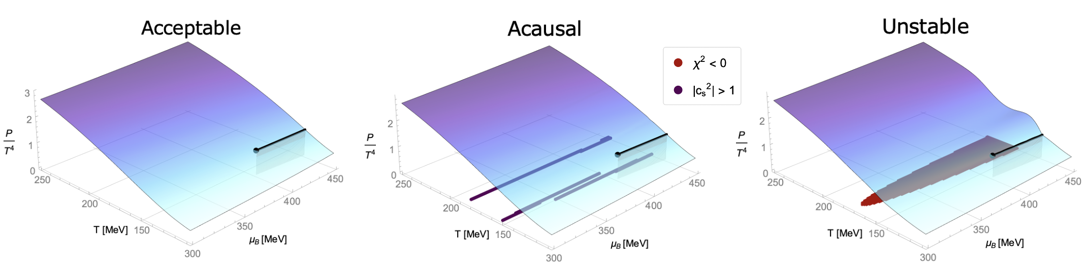
Figure 1: Different realizations of the EoS pertaining to the three thermodynamic stability classes. The black line illustrates the first-order transition line, which ends at the critical point. The projected $T-\mu_{B}$ plane is also shown, on which the points where some pathological behavior appears are highlighted (purple corresponding to causality violations and red to negativity of the second-order baryon susceptibility).

The first map yields the pressure as a function of temperature and chemical potential. The second map determines if the resulting EoS is acceptable or not. Fig. 1 illustrates how different realizations of the EoS can present pathological behaviors.

We use both the input parameters and a dimension-reduced version of the pressure for training. It is important to investigate how the choice of training – on either the input parameters or pressure – map to stable EoS, because the two spaces relate to thermodynamic stability in fundamentally different ways. The key difference is that models trained on input parameters are constrained to this particular formulation of the EoS, while training on the pressure can yield ML models that generalize to any QCD EoS. However, we will not test how training on the pressure can be applied to alternative EoS since that is beyond the scope of this paper. In this work, we focus on establishing that it is possible to train ML classifiers that identify viable EoS quickly and with high accuracy. Below we discuss how the labels for the training set were created and how the data was processed prior to training.

III.1 Thermodynamic Stability

There are four free parameters that emerge from our construction of the EoS that can lead to pathological behavior. Hence, thermodynamic stability needs to be verified at the end of the procedure, once all thermodynamic quantities have been calculated. In general, we require the positivity of the pressure, entropy and baryon density, the second order baryon susceptibility ($\chi_{2}^{B}$), and the heat capacity $(\partial S/\partial T)_{n_{B}}$

$$P,s,\varepsilon,n_{B},\chi_{2}^{B},\left(\frac{\partial S}{\partial T}\right)_{n_{B}}>0\,\,,$$ (14)

which follows from the requirement that entropy should be maximized in equilibrium. We also require that the speed of sound squared must be both positive and bounded by causality

$$0\leq c^{2}_{s}\leq 1.$$ (15)

All of these must be satisfied at every point in the $(T-\mu_{B})$ plane. As mentioned in Section I, there are two options for training data – using the pressure, which encodes all the information regarding stability and causality, or the input parameters which map to a particular EoS. In both cases, some number of training samples need to be generated. These must go through the numerical differentiation and grid checking process to be labeled. Generating a single EoS with a complete thermodynamic description and label can take between 1.2-4 times as long as generating the pressure only. While this approach reduces computation time and memory requirements, the difference is even more dramatic if we use the input parameters as training data. No calculation is required for generating an unlabeled sample of the parameter space – we simply select points from the parameter space grid. The runtime is negligible compared to how long it takes to generate a realization of the EoS.

III.2 Preprocessing

Let us first discuss the dimensionality of our problem at each stage of the mapping described in Eq. (13). We define a single set of input parameters as a training vector $\vec{\Omega}_{(i)}=(\mu_{B(i)},\alpha_{\textrm{diff(i)}},w_{(i)},\rho_{(i)})$. Each $\vec{\Omega}_{(i)}$ is four-dimensional, so we do not need to apply dimensionality reduction techniques. The only pre-processing required is a standard scaling of the distribution of $\vec{\Omega}_{(i)}$ in the training set. This is necessary to ensure the different features are compared along the same scale, to avoid artificially introducing differences in the data, and to ensure the pool and test set are analyzed with respect to the training distribution. We discuss the role of the pool, training, and test sets in the next section.

In the next step of our mapping, $P(T,\mu_{B})$ has dimensions corresponding to the grid size of the EoS. In our case, the limits are

$$30\leq\, T\;[\rm MeV] \,\leq 800$$ (16)

$$0\leq\, {\mu_{B}}\;[\rm MeV] \,\leq 450$$ (17)

with a step size of $1$ MeV in both directions. Thus, $P(T,\mu_{B})$ is a table of dimension $451\times 771$. A grid of this magnitude is not optimal for machine learning. We use the standard technique of Principal Component Analysis (PCA) Jolliffe2002 ; Hastie09 ; Murphy2012 to create a dimension-reduced projection of the original matrix defined by $P(T,\mu_{B})$. We check how many components are needed to account for most of the variance present in the pressure; our results show that the two-component projected matrix accounts for over 99% of the variance in nearly all cases. Based on these findings, we define a new variable, $P^{*}$, with about 1500 features corresponding to the two columns of the two-dimension projection matrix from the PCA. This is by no means a low-dimension feature space, but it is easily handled by most machine learning algorithms.

The final stage of the learning pipeline classifies the input EoS as either acceptable, unstable and acausal, or acausal, with no signs of instability (3-dimensional output space).

IV Sampling

Since the parameter space for our model is continuous, we first discretize it by defining a grid in each parameter within a range of interest. The bounds and step-sizes for each parameter are summarized in Table  1. The bounds in $\mu_{BC}$ are motivated by lattice QCD constraints. The upper bound is informed by the fourth order Taylor expansion of lattice data used in Ref. Parotto:2018pwx , which breaks down at $\mu_{B}\gtrapprox 450$ MeV. While there is no limit to how close the critical point can be placed to vanishing chemical potentials by construction, lattice results indicate that the region $\mu_{B}\lessapprox 2T$ is not likely to contain a critical point Bazavov:2017dus . The lower bound in $\mu_{BC}$ is loosely determined by these results and based on lattice calculations for the crossover temperature $T_{0}\simeq 155$ MeV at $\mu_{B}=0$ Aoki:2009sc ; Borsanyi:2010bp ; Bhattacharya:2014ara ; Bazavov:2011nk . Since the curvature of the deconfinement transition line appears to be negative, we can safely expect that the critical temperature $T_{C}\lessapprox 155$ MeV. Lattice results then roughly rule out $\mu_{BC}\lessapprox 300$ MeV, but we extend this lower bound down to $220$ MeV to accommodate for possible uncertainties in these values. The other three parameters are specific to the linear map assumed in the construction of the EoS and no arguments from first-principles constrain their values, so the corresponding bounds are designed to span all possible behavior. Broadly speaking, it was observed already in Ref. (Parotto:2018pwx, ) that, with all other parameters fixed, when a certain choice of $w$ was found to be pathological, then the same occurred for all $w^{\prime}<w$. The opposite behavior was observed for a pathological EoS with a certain $\rho$ – with all other parameters fixed, all $\rho^{\prime}>\rho$ were pathological.

Every time a model is initialized, an initial training and test sets are generated from the parameter grids, containing 350 and $\sim 20,000$ labeled realizations of the EoS, respectively. The initial training set is chosen randomly at the beginning of each training cycle from the remaining points (which constitute the pool set), so that there is no overlap between test and training sets. The initial training set contains the first labeled realizations from which the model will learn. More instances are added to the training set with each iteration. The test set remains the same throughout all training iterations and it is used to check the accuracy of the model at each stage.

Once the initial training set $\mathcal{L}_{0}$ has been determined, we take the following steps:

1. A machine learning model is trained on $\mathcal{L}_{0}$.

2. The model makes a prediction on the test set and its performance is recorded (for reporting purposes only).

3. The model is then evaluated on $\mathcal{U}_{0}$, the pool set, which contains all points in neither $\mathcal{L}_{0}$ nor the test set. These points are unlabeled.

4. Using some selection criterion, a query is generated. This means a size-$k$ pool of points is selected from $\mathcal{U}_{0}$ according to some distribution, and a label is provided for these points.

5. The training and pool sets are updated. The new training set $\mathcal{L}_{1}$ contains $\mathcal{L}_{0}$ and the queried points, which are now missing from the updated pool set $\mathcal{U}_{1}$.

6. The model is trained on $\mathcal{L}_{1}$ and steps 2-5 are repeated until a stopping criterion is met.

Table 1: Ranges and step-sizes used to generate EoS for training and testing.

	Min.	Max.	Step size
$\mu_{BC}$	220 MeV	420 MeV	20 MeV
$w$	0.1	10.0	0.5
$\rho$	0.1	10.0	0.5
$\alpha_{\textrm{diff}}$	$-180\degree$	$180\degree$	$5\degree$

We expect to see the average recorded accuracy increase as sample size increases until the model converges at some maximum accuracy value, or until resources for generating labeled instances have been exhausted. This should happen independently of the selection criterion. However, if labeled samples are difficult (e.g. computationally costly) to generate, an improved sampling method can provide an advantage in terms of how many samples are needed to achieve a target performance. Active learning methods seek to increase the performance of learning algorithms with fewer samples by allowing models to choose which data to learn from.

We test the performance of our models using both random sampling and active learning. We draw our samples in a pool-based fashion, meaning queries consist of size-$k$ samples drawn from $\mathcal{U}$. In the random case, the samples are randomly pulled from $\mathcal{U}$ assuming a uniform distribution. Margin-based queries select the k points currently in the pool set $\mathcal{U}$ with the smallest margin values, where the margin $M$ is defined as in Ref. scheffer2001active ,

$$M=P(\hat{y}_{1})-P(\hat{y}_{2})$$ (18)

and $\hat{y}_{1}$ and $\hat{y}_{2}$ are the first and second most probable class labels under the current model, with corresponding probabilities $P(\hat{y}_{i})$. Therefore, this sampling method favors points with a small margin, meaning the classification is ambiguous, whereas points where one class is clearly preferred do not get labeled. Using this query strategy avoids wasting resources on instances the model already understands how to classify in favor of those that are still ambiguous. It is important to note that, although we make the choice to fix each query at $k=200$ samples (i.e. each iteration in training represents the same increase in training set size) that choice is in principle arbitrary.

V Model training and selection

The main goal in the model training and selection stage is to gauge what is necessary to create a strong EoS classifier – how much data is needed, how to sample from the available data, and how to make a choice for the classification algorithm. Generally, the amount of data needed is measured according to the accuracy of the classifier on the test set, but it could also be limited by computational resources. The preference for a sampling method is determined based on whether random sampling or active learning reached higher accuracy at a lower number of samples (e.g. 95% test set accuracy rate at 5,000 samples is better than a 95% rate at 7,000 samples). The best model is then the combination of algorithm plus sampling method that reaches the highest accuracy rate with the fewest possible samples.

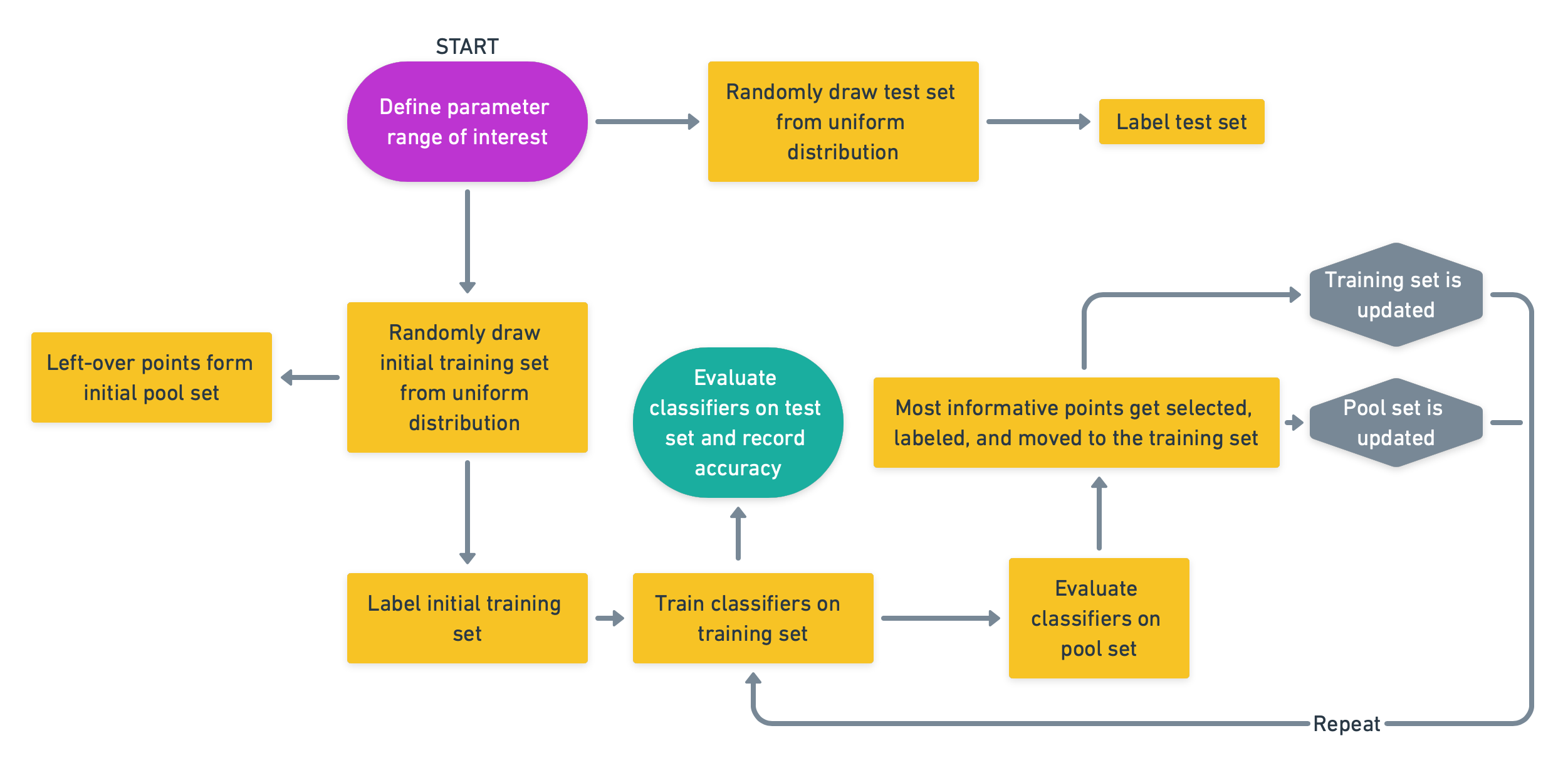
Figure 2: Flowchart of model development and testing. From an initial grid of interest, three sets are created – an initial training set and a test set (each containing labeled realizations of the EoS), and a pool set, which contains all the points outside the test or initial training sets. With each iteration the performance of the classifier is recorded, and a new set of points from the pool set is labeled and moved to the training set.

We select three classification algorithms as mentioned in Sec. I – SVM, RF, and KNN – and train them using the sampling framework described in Sec. IV. The sampling and training procedures are summarized in Fig. 2. We used the open source library scikit-learn scikit-learn and the publicly available implementation in Ref. cohen2018activelearningtutorial to develop the code used in this work. Sampling is performed as outlined in Section IV. Additionally, at each training step, the model’s hyperparameters are optimized over a random grid search using 5-fold cross-validation on the training set. This step is crucial since the training set changes with each iteration and the hyperparameters need to be readjusted. Details about the hyperparameters for each model can be found in the documentation for Ref. scikit-learn , and the specific grid search used in this work is available in the source code mroczekgithub2022 .

For RF and KNN methods, training is set to stop at 10,000 samples, regardless of accuracy levels, in order to constrain computational expenses. For SVM models, the run-time scales with the cubic power of the number of training samples, and training is set to stop at 2,500 samples instead. To deal with the cold start problem we randomly select a new initial training set with each new run. The cold start problem refers to the expected model instability when faced with data scarcity, which is common when using active learning on a small sample Yuan20 ; Grimova18 . We also do not throw away any labels during training. Once a point is labeled, the label is kept and recycled if the same point is called again by the sampling algorithm in a different run.

We perform a total of 25 experiments – 5 repetitions for each of the learning algorithms (RF, SVM, KNN), using either random sampling or active learning on the input parameter vector ${\vec{\Omega}}_{(i)}$, and 5 repetitions for RF using either random sampling or active learning on the dimension-reduced version of the pressure $P^{*}$. For each combination, we take the mean accuracy at each training set size with a 1$\sigma$ deviation band.

VI Results

This section is divided into two parts – the first addresses the development and selection of an adequate machine learning model for the EoS classification problem, as well as the performance of active vs. traditional learning implementations. Secondly, we discuss the deployment of the best-performing model, what is learned about the correspondence between EoS parameter space and stability classes, and implications for the modeling of heavy-ion collisions and experimental searches for the QCD critical point.

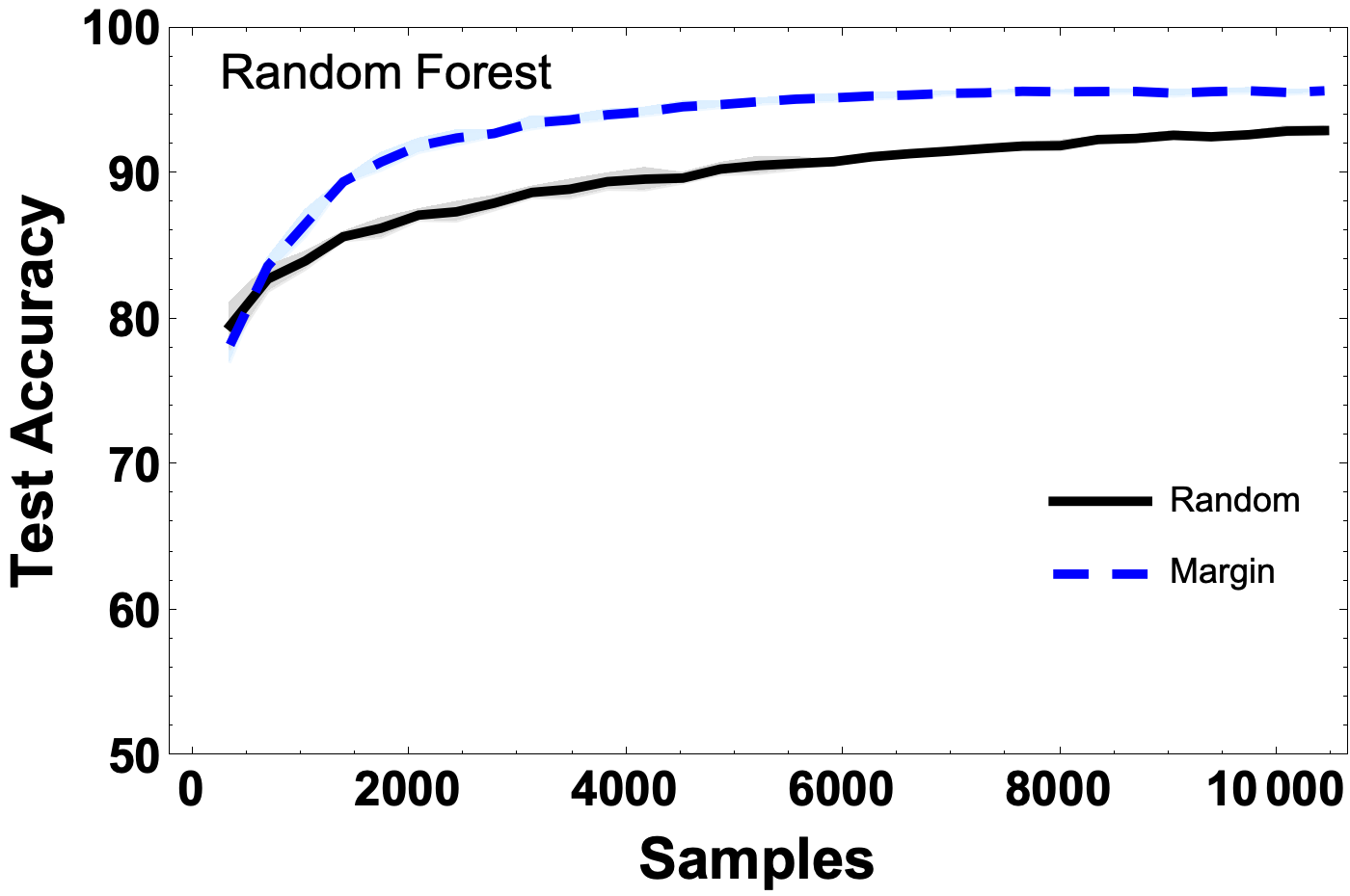
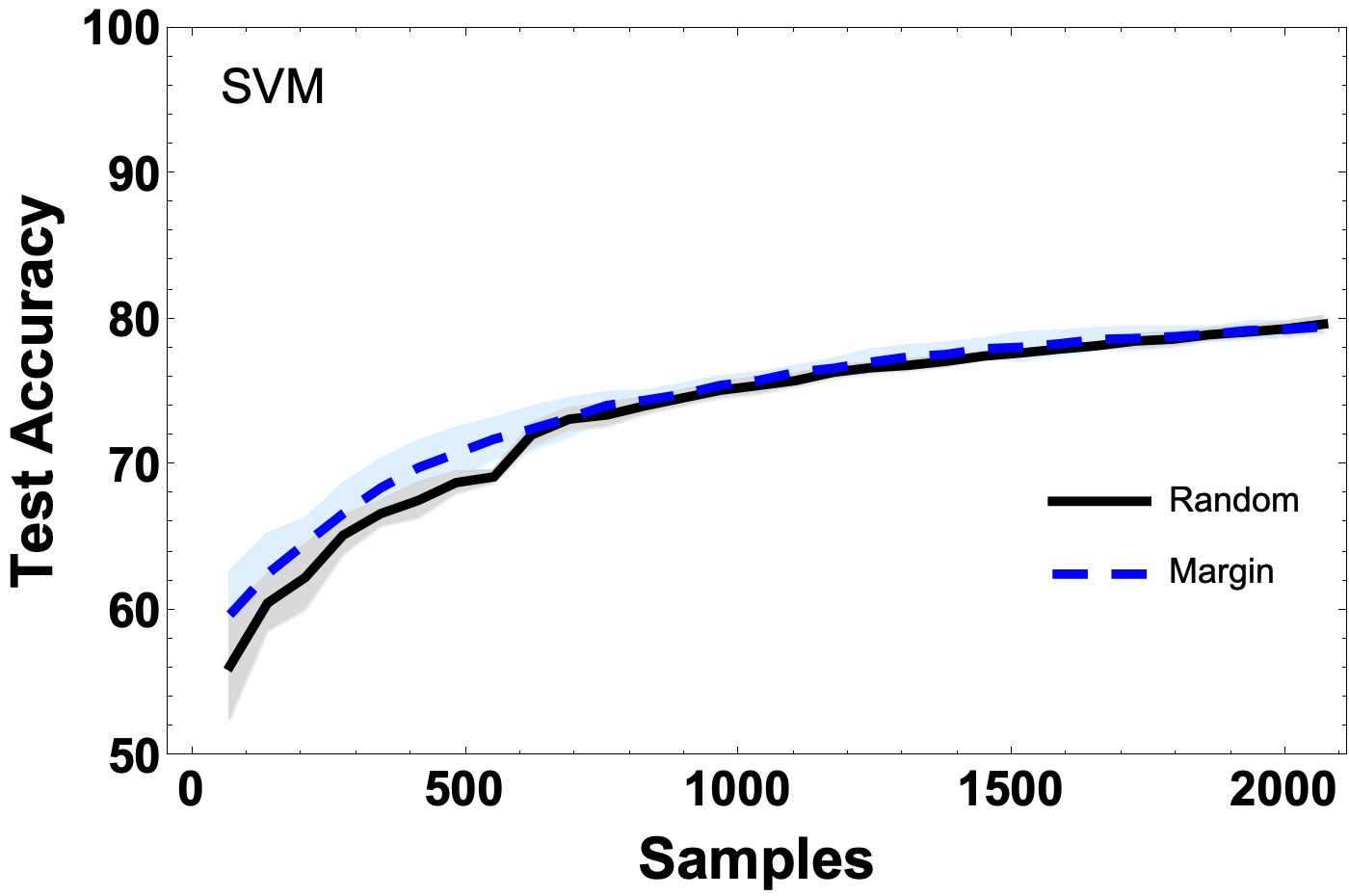
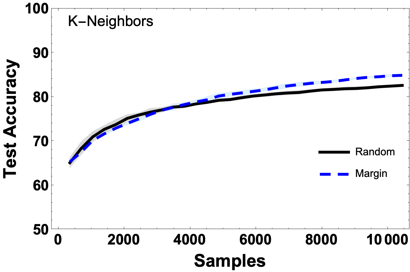
Figure 3: Average performance on the test set as a function of training set size. The black lines correspond to the performance of models trained using random sampling and the dashed blue lines correspond to models trained using active learning. The bands show 1$\sigma$ deviations from the average.

VI.1 Model development

The primary aspect of developing a machine learning model is to track how performance evolves during training. Fig. 3 shows test accuracy as a function of training set size for each class of models trained on only the input $\vec{\Omega}_{(i)}$ data (recall that we distinguish this from training directly on the EoS itself that is signified by $P^{*}$). The solid and dashed lines represent the average behavior for a class of models across 5 runs with random sampling and active learning, respectively, and a corresponding 1$\sigma$ uncertainty band. Generally, a performance measure, which in this case is the recorded test set accuracy, is expected to improve on average as the number of training samples increases. We also re-emphasize that, during training, the model is completely blind to the test set and there is no overlap between test and training points. From Fig. 3, it is clear that active learning provides a significant advantage for RF and KNN models. In the SVM case, there is an initial advantage that vanishes when the training set reaches a size of $\sim$700 samples.

We are interested in the combination of input data, sampling, and learning algorithm that performs best given the constraints set for label acquisition. From Fig. 3, we see that RF coupled to active learning clearly outperforms other models, with test set accuracy quickly converging around 96% and exhibiting small variability. This agrees with our understanding of the benefit behind ensemble methods, where voting over multiple (nearly uncorrelated) models tends to reduce the bias and the variance component of the error significantly, see for example Refs. Hastie09 ; Murphy2012 ; Bishop2006 ; Goodfellow2016 ; Mehta2019 for an in-depth discussion on the bias-variance trade-off in machine learning.

Although a consistent final accuracy of 96% is good enough for most applications of learning algorithms, we wanted to investigate if an even higher accuracy could be achieved using the dimension-reduced pressure $P^{*}$ as the training data. Because generating $P^{*}$ and training models using it as input is significantly more computationally expensive than the previous case, we limit this analysis to RF algorithms. This is expected considering the complexity cost behind SVM and KNN (for small K). As an example, SVMs are mathematically represented by a convex optimization problem. Ensemble methods like random forests, gradient boosting, bagging and others Hastie09 ; geron2022 normally use shallow decision trees as weak learners. Such decision trees are easy to train and require normally less CPU cycles than convex optimization problems like SVMs, which involve affine transformations with dense matrices.

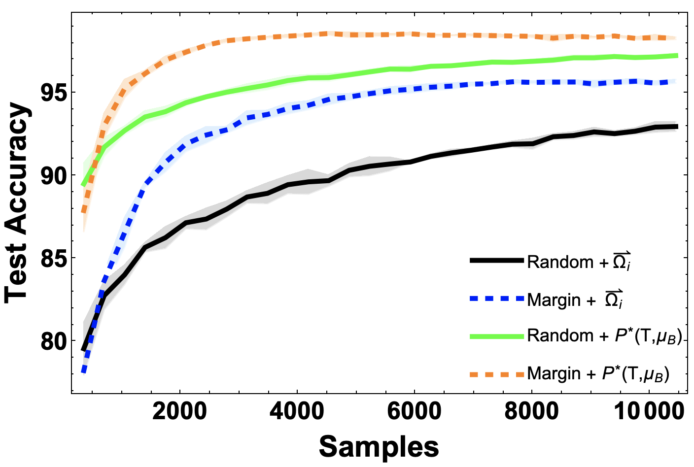
Figure 4: Accuracy on the test set for RF models trained on input parameters coupled to random (solid black) and margin (dashed blue) sampling methods. This is compared to RF models trained on the transformed pressure coupled to random (solid green) and margin (dashed orange) sampling methods.

We compare the performance of RF models using different training data in Fig. 4, which shows the accuracy on the test set as a function of the training set size during training. The dashed orange and solid green lines correspond to margin and random sampling, respectively, using $P^{*}$ as input. The dashed blue and solid black lines correspond to margin and random sampling, respectively, using $\vec{\Omega}_{(i)}$ as input. The matching bands represent a 1$\sigma$ deviation from the mean performance over 5 runs. For both input classes, active learning outperforms random sampling. Surprisingly, when RF algorithms are trained using $P^{*}$, they outperform RF models trained on $\vec{\Omega}_{(i)}$ using active learning in all stages of training. The classifier performs even better when trained on $P^{*}$ with active learning, consistently achieving nearly perfect accuracy with under 3,000 samples in the training set.

This increase in accuracy is likely due to the nature of the map between the different input spaces and the EoS classes. The map between $\vec{\Omega}_{(i)}$ and the stability classes is highly non-linear, whereas in $P^{*}$ space, the transition between classes is likely simpler to model in terms of input variables. Regardless, a strong classifier can be achieved with either set of input data. Using $P^{*}$ sacrifices the computational advantage over non-ML classification for near perfect classification accuracy, while models trained on $\vec{\Omega}_{(i)}$ peak at slightly lower accuracy, but with a significantly lower computational cost. We discuss execution-time benchmarking in detail in Sec. VI.2.1.

The summary of predictions on the test set is given by the confusion matrix sammut2010 of the model. In Fig. 5, we show the confusion matrix for both classes of models with active learning, where the columns represent the true class (as calculated thermodynamically), and the rows indicate the class predicted by the model. We normalize the number of points in each entry by the total number of points in the test set, and show the corresponding percentage. The diagonal elements are the percentage of points that belonged to a certain class and were classified correctly by the model. Correspondingly, the off-diagonal elements quantify the percentage of points in the test set that were misclassified by the model.

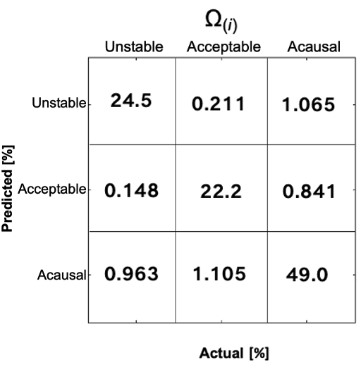
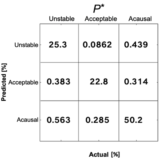
Figure 5: Confusion matrix averaged over the final random forests models’ performance on the test set, after training with $\Omega_{(i)}$ (top) or $P^{*}$ (bottom).

From Fig 5, we see that acausal EoS are the most problematic class for models trained on $\vec{\Omega}_{(i)}$. Out of the average 4.33% of points that were misclassified, an average total of 2.07% were incorrectly predicted to be acausal, while another average 1.906% of points that were acausal ended up misclassified as either acceptable or unstable. Combined, acceptable/unstable points being incorrectly classified as acausal and, on the other hand, acausal points being incorrectly classified as acceptable/unstable account for 92% of misclassifications on average. If we break down the confusion between acausal and acceptable/unstable individually, we see that most incorrectly classified acausal points are, in reality, unstable, and vice-versa.

In the context of the EoS parameter space, this means that there is a clear distinction between acceptable and acausal/unstable EoS, but the boundary between acausal and unstable can become fuzzy in certain regions. In this aspect, using $P^{*}$ as training input seems to help, but not significantly. As shown in Fig 5, out of the average 2.07% of points that were misclassified, confusion in acausal classifications accounts for 77.4% of the mistakes.

In practice, the most important aspect of the confusion matrix analysis is to evaluate the prevalence of false positives/negatives. A false positive would be an EoS that is unstable/acausal, but gets incorrectly classified as acceptable. A false negative is an acceptable EoS that gets incorrectly classified as unstable/acausal. From Fig. 5, we see that the false negative and positive rates for the models trained on $\vec{\Omega}_{(i)}$ are on average 1.316% and 0.989%, respectively. In the $P^{*}$ cases, the average rates are 0.371% for false negatives and 0.697% for false positives.

The incidence of false positives/negatives for the class of models trained on $P^{*}$ is about half of those trained on the input vectors, but in either case these rates are low enough for most applications. In general, models taking in $P^{*}$ are more suitable for analyses that require knowledge of a specific point, since the overall accuracy is higher. However, models trained on $\vec{\Omega}_{(i)}$ still provide an accurate description of the EoS parameter space and class structure.

VI.2 Model Deployment

In addition to training and comparing the performance of different classes of models, we illustrate a deployment framework by analyzing the features of the EoS parameter space relevant to experimental searches for the critical point. The analysis was done using the top performing model in terms of classification accuracy and execution time, namely random forests trained with active sampling and input vectors $\vec{\Omega}_{(i)}$. From here on, we will refer to this model as RF${}^{A}_{\Omega}$, where RF stands for random forests, A for active learning, and $\Omega$ refers to the type of training data.

VI.2.1 Execution time benchmarking

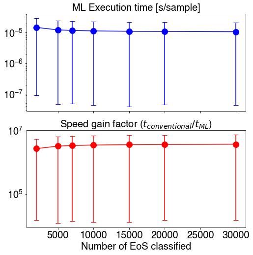
Figure 6: Top panel: execution time per sample on a log scale as a function of the total number of samples with ML classification. Bottom panel: speed factor gained using ML versus conventional classification. In both cases the error bars represent a 68% confidence interval based on jackknife resampling of 50 samples.

One of the important metrics when choosing a model for deployment is accuracy. The RF${}^{\textrm{A}}_{\Omega}$ model yields a final test set accuracy of 96.772 %. This is not as high as the models that were trained on $P^{*}$. However, it is important to also keep track of the execution time. Machine learning assisted classification, if implemented appropriately, should yield a significant computational advantage. Without ML assistance, the classification of EoS stability is $\mathcal{O}(1-2)$ in seconds. The execution time of ML-assisted classification can be calculated as a per sample rate, classifying a certain number of samples in bulk, then dividing the total execution time by the total number of samples. This is shown in the top panel of Fig. 6, which displays the execution time in seconds per sample for RF${}^{\textrm{A}}_{\Omega}$ classification as a function of the number of EoS classified. In order to test the robustness of the model, we repeat this rate calculation 50 times and show the 68% confidence interval based on jackknife resampling. The model consistently performs at the microsecond scale.

In the bottom panel of Fig. 6, we show the speed gain factor as a function of the number of EoS classified. This was calculated by dividing the ML execution time per sample by the non-ML classification time per sample. The same statistical methods were used for constructing the confidence intervals. RF${}^{\textrm{A}}_{\Omega}$ assisted classification consistently provides a computational advantage of 5-6 orders of magnitude.

VI.2.2 EoS Stability Analysis

The speed and high accuracy of RF${}^{\textrm{A}}_{\Omega}$ allow us to map the stability of the EoS as a function of input parameters in fine detail. These parameters relate to key physical properties of the QCD critical point. As discussed Sec. II, $\alpha_{\textrm{diff}}$ represents the angular separation between Ising axes $(r,h)$ in the mapping to QCD variables, $w$ globally scales the Ising axes – i.e. the critical region – and $\rho$ stretches the critical region along the transition line ($\mu_{B}$ direction).

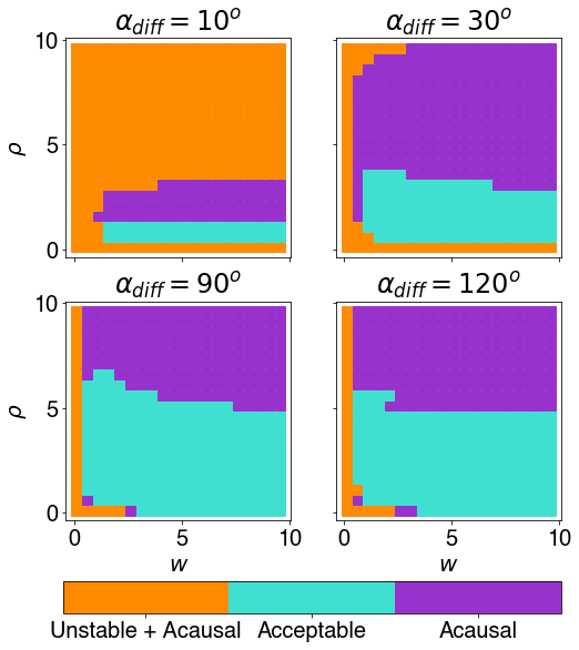
Figure 7: Stability and causality regions on the $w-\rho$ plane for different $\alpha_{\textrm{diff}}$ values at fixed $\mu_{BC}=400$ MeV. As the angular parameter moves away from orthogonality, the stability region shrinks. An upper limit appears for $\rho$, which drives EoS to acausal regions when too large.

In Fig. 7, we fix $\mu_{B}=400$ MeV and determine the stability/causality of the EoS for different values of the angular parameter $\alpha_{\textrm{diff}}$ as a function of the scaling parameters $w$ and $\rho$ on a grid much finer than previous calculations Parotto:2018pwx . From Fig. 7 it can be inferred that the stability region in the $w-\rho$ plane shrinks as the angular parameter moves away from orthogonality, and that there is a hard limit on the value of $\rho$, which drives the EoS to acausal regimes when too large. Hence, under the current mapping, the critical region cannot be too large in the $\mu_{B}$ direction.

The exact value of the $\rho$ stability cut-off depends strongly on the value of $\alpha_{\textrm{diff}}$, but not as much on the global scaling of the critical region determined by $w$. These results reflect the underlying physics of the model Mroczek:2020rpm . The EoS with critical contributions is matched to lattice QCD data by construction, and these parameters can stretch the critical region along the transition line to the point where the EoS cannot be simultaneously acceptable and consistent with lattice QCD. If either $\alpha_{\textrm{diff}}$ or $\rho$ spreads the critical region too broadly across $\mu_{B}$, the EoS will become acausal. Stability and causality also depend on $\mu_{BC}$, which is discussed below and in Section VI.3.

Another point of interest is to maximize the overall size of the critical region. This is reflected by the minimum value of $w$, to which to the overall size of the critical region is (mildly) inversely proportional. In general, one has $\Delta\mu_{B}\Delta T\sim w^{-2/7}$ Mroczek:2020rpm , where $\Delta\mu_{B},T$ are the corresponding sizes of the critical region in the $T$ and $\mu_{BC}$ directions. Hence, despite the overall size of the critical region only being midly affected by $w$, it determines the largest possible critical region for a particular choice of $\mu_{BC}$, $\rho$, and $\alpha_{\textrm{diff}}$. This analysis is shown in Fig. 8, which displays the smallest acceptable value $w=w_{0}$ for different values of $\mu_{BC}$ and fixed $\rho=2$ as a function of $\alpha_{\textrm{diff}}$. We see that, as $\alpha_{\textrm{diff}}$ moves away from $\pm$ 90${}^{\textrm{o}}$ (orthogonal Ising axes), it drives the value of $w_{0}$ up. In addition, as $\alpha_{\textrm{diff}}\rightarrow 0$, stability disappears entirely. The band where no EoS are possible shrinks as we move $\mu_{BC}$ to larger values, as would be expected since large $\mu_{BC}$ interferes the least with lattice results at $\mu_{B}=0$. Most importantly, we see that regions of low $w_{0}$ appear at values of $\alpha_{\textrm{diff}}$ closer to $90^{\textrm{o}}$, meaning that these regimes are compatible with a larger critical region. When $\mu_{BC}$ is larger, the low $w_{0}$ regions extend for longer in $\alpha_{\textrm{diff}}$, because moving the CP away from $\mu_{B}=0$ allows for a larger CP to still be consistent with the matching to lattice QCD. To summarize, we find that placing the critical point at larger $\mu_{BC}$ guarantees the most flexibility in the possible size and shape of the critical region. However, even when $\mu_{BC}$ is large, the Ising axes cannot come too close together without causing pathological behavior.

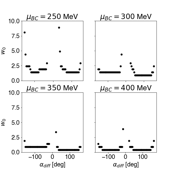
Figure 8: Smallest possible value $w_{0}$ (largest global scaling of the critical region thermodynamically allowed) for different values of $\mu_{BC}$ and $\rho=2$ as a function of $\alpha_{\textrm{diff}}$.

VI.3 Correlations between input parameters in acceptable EoS

In the process of developing and training the ML models presented in this work, nearly 40k realizations of the BEST EoS were labeled. The pool of labeled EoS includes samples taken randomly and with active learning. Since active queries oversample along the boundary, this collection of EoS should strongly reflect the true stable and causal regions. By selecting only the acceptable EoS from this pool, we can gain insight on the distribution and correlations between input values in the stability/causality windows. The analysis of the acceptable training samples is presented in this work as a tool complementary to the ML models because the training data reflects the true distributions and correlations between parameters for acceptable EoS. These samples should be studied because they display the trends ML classification should follow, aside from providing a general intuition for the regime of thermodynamic validity of the EoS model.

The histogram for each input parameter is shown along the diagonal in the corner plot in Fig. 9. We see acceptable EoS are more likely to stem from larger values of $\mu_{BC}$, values of $\alpha_{\textrm{diff}}$ close to $90^{\textrm{o}}$, and lower $\rho$. There is not a strong dependence on $w$, but the number of acceptable EoS decreases for $w\lesssim 1$. The observations are in line with general arguments on the size and shape of the critical region Mroczek:2020rpm . The peak at $\rho\approx 2.0$ is likely due to active learning, since this seems to be the point where EoS in the intermediate angle regime (10${}^{\textrm{o}}$ $\leq\alpha_{\textrm{diff}}\leq$ 60${}^{\textrm{o}}$) become acausal. These findings are consistent with what was found with ML-assisted classification using RF${}^{A}_{\Omega}$.

The off-diagonal elements of Fig. 9 contain the pair-wise density correlations between input parameters. As expected, $\alpha_{\textrm{diff}}$ correlates strongly with other input parameters – a CP further away from $\mu_{B}=0$ and smaller $\rho$ allow for smaller angles. However, $\alpha_{\textrm{diff}}$ is always above $5^{\textrm{o}}$, even when $\rho$ is small, and $\rho$ is always below 5.0-6.0, even when $\alpha_{\textrm{diff}}$ is not small. Thus, there is a limit for $\alpha_{\textrm{diff}}$ and $\rho$ in the current implementation of this model, since we cannot place the critical point at a larger value than $\mu_{BC}=420$ MeV due to limitations from lattice QCD. There is not a strong correlation between stability and $w$, because it is always possible to make the critical region small enough to suppress unstable behavior. Furthermore, we observe that larger critical regions ($w\lessapprox 1$) only appear for $\mu_{BC}>300$ MeV. This confirms the trends found by RF${}^{A}_{\Omega}$ for the subsets of the parameter space discussed in Section VI.2.2.

In summary, $\mu_{BC}\gtrapprox 300$ MeV provides the most freedom, but it always holds that $\rho\lessapprox 5.0$ and $\alpha_{\textrm{diff}}\gtrapprox 5.0^{\textrm{o}}$ under the current mapping. Recall that any pathological behavior of the EoS is due to tension with lattice calculations. This is model-dependent because of the choice of mapping between Ising and QCD variables and the truncation of the lattice Taylor expansion. Changing either would affect the quantitative results discussed in this work, which are specific to the EoS presented in Ref. Parotto:2018pwx .

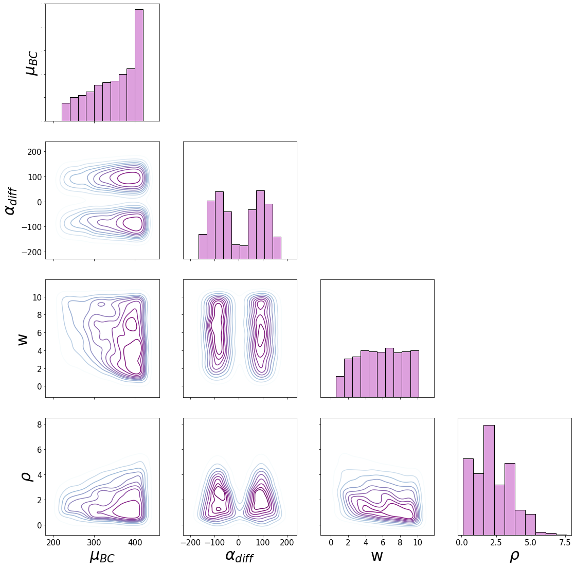
Figure 9: Off-diagonal: pair-wise correlations between input parameters for acceptable EoS in the combined training set. Each plot shows the density distribution for pairs of input parameters. Diagonal: Histograms for each parameter and its distribution in the class of acceptable EoS.

VII Conclusions

The BEST collaboration EoS relies on a non-universal linear map of 3D Ising model variables onto the QCD phase diagram, which contains four free parameters. A subset of the resulting four-dimensional parameter space leads to unstable and/or acausal realizations of the EoS. In this work, we built a machine learning framework that incorporates active learning to guide the model towards the most important regions in the input parameter space; this helps to efficiently rule out unphysical EoS with high accuracy. In addition to mapping the stability and causality of the EoS as a function of the input parameters across the entire available parameter space, we find that certain mapping parameters are constrained to $\alpha_{\textrm{diff}}\gtrapprox 5^{\textrm{o}}$ and $\rho\gtrapprox 5$. Additionally, a strong preference for a critical point at large baryon chemical potentials $\mu_{BC}$ is shown, especially when the critical region is large. Low $\mu_{BC}$ can only coexist with significantly smaller critical regions. Although these findings are quantitatively strongly dependent on the actual implementation of the BEST EoS, their qualitative nature is likely to be quite general, as it essentially stems from the (in)compatibility of the universal critical behavior and first-principle lattice QCD results.

The insights presented in this work can be used in future hydrodynamic studies of the evolution of matter created in ultra-relativistic heavy-ion collision experiments at low beam energies. Currently for heavy-ion collisions, it is not possible to directly compare the EoS to experimental data. Instead, one must run relativistic viscous hydrodynamic simulations with a large number of free parameters that are then directly compared to experimental data. The free parameters are constrained using a combination of emulators and Bayesian analysis Pratt:2015zsa ; Bernhard:2016tnd ; Bernhard:2019bmu ; JETSCAPE:2020mzn ; Nijs:2020roc , which are limited by the enormous amount of computational time required to run a single parameter set. The results presented here significantly cut down the input parameter space, allowing for tighter priors in a potential Bayesian analysis comparing heavy-ion hydrodynamics simulations to experimental data.

This is the first time that active learning has been employed in the context of heavy-ion collisions. We demonstrated that active learning can significantly reduce sampling requirements for training classifiers to search for acceptable EoS. Because of the speed and accuracy we reached in our framework using active learning, our methodology promises to be useful for a number of problems in the field of heavy-ion collisions. Additionally, the machine learning pipeline developed in this work is generic enough that it can be applied to any EoS with a parameter-space-to-class correspondence.

- [1] Y. Aoki, G. Endrodi, Z. Fodor, S. D. Katz, and K. K. Szabo. The Order of the quantum chromodynamics transition predicted by the standard model of particle physics. Nature, 443:675–678, 2006.
- [2] Mikhail A. Stephanov. QCD phase diagram and the critical point. Prog. Theor. Phys. Suppl., 153:139–156, 2004.
- [3] Misha A. Stephanov, K. Rajagopal, and Edward V. Shuryak. Signatures of the tricritical point in QCD. Phys. Rev. Lett., 81:4816–4819, 1998.
- [4] J. Adam et al. Nonmonotonic Energy Dependence of Net-Proton Number Fluctuations. Phys. Rev. Lett., 126(9):092301, 2021.
- [5] M. S. Abdallah et al. Measurements of Proton High Order Cumulants in 3 GeV Au+Au Collisions and Implications for the QCD Critical Point. 11 2021.
- [6] Jaroslav Adam et al. Flow and interferometry results from Au+Au collisions at GeV. Phys. Rev. C, 103(3):034908, 2021.
- [7] Ani Aprahamian et al. Reaching for the horizon: The 2015 long range plan for nuclear science. 10 2015.
- [8] Adam Bzdak, Shinichi Esumi, Volker Koch, Jinfeng Liao, Mikhail Stephanov, and Nu Xu. Mapping the Phases of Quantum Chromodynamics with Beam Energy Scan. Phys. Rept., 853:1–87, 2020.
- [9] Veronica Dexheimer, Jorge Noronha, Jacquelyn Noronha-Hostler, Claudia Ratti, and Nicolás Yunes. Future physics perspectives on the equation of state from heavy ion collisions to neutron stars. J. Phys. G, 48(7):073001, 2021.
- [10] Akihiko Monnai, Björn Schenke, and Chun Shen. QCD Equation of State at Finite Chemical Potentials for Relativistic Nuclear Collisions. Int. J. Mod. Phys. A, 36(07):2130007, 2021.
- [11] Xin An et al. The BEST framework for the search for the QCD critical point and the chiral magnetic effect. Nucl. Phys. A, 1017:122343, 2022.
- [12] J. Adamczewski-Musch et al. Proton-number fluctuations in =2.4 GeV Au + Au collisions studied with the High-Acceptance DiElectron Spectrometer (HADES). Phys. Rev. C, 102(2):024914, 2020.
- [13] Paolo Parotto, Marcus Bluhm, Debora Mroczek, Marlene Nahrgang, Jacquelyn Noronha-Hostler, Krishna Rajagopal, Claudia Ratti, Thomas Schäfer, and Mikhail Stephanov. QCD equation of state matched to lattice data and exhibiting a critical point singularity. Phys. Rev. C, 101(3):034901, 2020.
- [14] J. M. Karthein, D. Mroczek, A. R. Nava Acuna, J. Noronha-Hostler, P. Parotto, D. R. P. Price, and C. Ratti. Strangeness-neutral equation of state for QCD with a critical point. Eur. Phys. J. Plus, 136(6):621, 2021.
- [15] Maneesha Pradeep, Krishna Rajagopal, Misha Stephanov, and Yi Yin. Freezing out critical fluctuations. In International Conference on Critical Point and Onset of Deconfinement, 9 2021.
- [16] Xin An, Gökçe Başar, Mikhail Stephanov, and Ho-Ung Yee. Evolution of Non-Gaussian Hydrodynamic Fluctuations. Phys. Rev. Lett., 127(7):072301, 2021.
- [17] Marlene Nahrgang, Marcus Bluhm, Thomas Schaefer, and Steffen A. Bass. Diffusive dynamics of critical fluctuations near the QCD critical point. Phys. Rev. D, 99(11):116015, 2019.
- [18] D. Mroczek, A. R. Nava Acuna, J. Noronha-Hostler, P. Parotto, C. Ratti, and M. A. Stephanov. Quartic cumulant of baryon number in the presence of a QCD critical point. Phys. Rev. C, 103(3):034901, 2021.
- [19] M. A. Stephanov. Evolution of fluctuations near QCD critical point. Phys. Rev. D, 81:054012, 2010.
- [20] Marlene Nahrgang, Stefan Leupold, Christoph Herold, and Marcus Bleicher. Nonequilibrium chiral fluid dynamics including dissipation and noise. Phys. Rev. C, 84:024912, 2011.
- [21] M. Stephanov and Y. Yin. Hydrodynamics with parametric slowing down and fluctuations near the critical point. Phys. Rev. D, 98(3):036006, 2018.
- [22] Marcus Bluhm et al. Dynamics of critical fluctuations: Theory – phenomenology – heavy-ion collisions. Nucl. Phys. A, 1003:122016, 2020.
- [23] Burr Settles. Active learning literature survey. Computer Sciences Technical Report 1648, University of Wisconsin–Madison, 2009.
- [24] Burr Settles. Active learning literature survey. 2009.
- [25] Hideitsu Hino Hino. Active learning: Problem settings and recent developments. CoRR, abs/2012.04225, 2020.
- [26] Pengzhen Ren, Yun Xiao, Xiaojun Chang, Po-Yao Huang, Zhihui Li, Brij B. Gupta, Xiaojiang Chen, and Xin Wang. A survey of deep active learning. ACM Comput. Surv., 54(9), oct 2021.
- [27] Sascha Caron, Tom Heskes, Sydney Otten, and Bob Stienen. Constraining the Parameters of High-Dimensional Models with Active Learning. Eur. Phys. J. C, 79(11):944, 2019.
- [28] Trevor Hastie, Robert Tibshirani, and Jerome Friedman. The elements of statistical learning: data mining, inference and prediction. Springer, 2 edition, 2009.
- [29] Kevin P. Murphy. Machine Learning: A Probabilistic Perspective. The MIT Press, Cambdridge, Massachusetts, 2012.
- [30] Christopher M. Bishop. Pattern Recognition and Machine Learning. Springer Verlag, Berlin, 2006.
- [31] Long-Gang Pang, Kai Zhou, Nan Su, Hannah Petersen, Horst Stöcker, and Xin-Nian Wang. An equation-of-state-meter of quantum chromodynamics transition from deep learning. Nature Commun., 9(1):210, 2018.
- [32] Rüdiger Haake. Machine and deep learning techniques in heavy-ion collisions with ALICE. 9 2017.
- [33] Jana Bielčíková, Raghav Kunnawalkam Elayavalli, Georgy Ponimatkin, Jörn H. Putschke, and Josef Sivic. Identifying Heavy-Flavor Jets Using Vectors of Locally Aggregated Descriptors. JINST, 16(03):P03017, 2021.
- [34] Jan Steinheimer, Longgang Pang, Kai Zhou, Volker Koch, Jørgen Randrup, and Horst Stoecker. A machine learning study to identify spinodal clumping in high energy nuclear collisions. JHEP, 12:122, 2019.
- [35] Yi-Lun Du, Daniel Pablos, and Konrad Tywoniuk. Deep learning jet modifications in heavy-ion collisions. JHEP, 21:206, 2020.
- [36] Amber Boehnlein et al. Artificial Intelligence and Machine Learning in Nuclear Physics. 12 2021.
- [37] Neelkamal Mallick, Sushanta Tripathy, Aditya Nath Mishra, Suman Deb, and Raghunath Sahoo. Estimation of Impact Parameter and Transverse Spherocity in heavy-ion collisions at the LHC energies using Machine Learning. Phys. Rev. D, 103(9):094031, 2021.
- [38] Yue Shi Lai, James Mulligan, Mateusz Płoskoń, and Felix Ringer. The information content of jet quenching and machine learning assisted observable design. 11 2021.
- [39] Yang-Ting Chien and Raghav Kunnawalkam Elayavalli. Probing heavy ion collisions using quark and gluon jet substructure. 3 2018.
- [40] Avik Sarkar and Dean Lee. Self-learning Emulators and Eigenvector Continuation. 7 2021.
- [41] Erik Buhmann, Sascha Diefenbacher, Engin Eren, Frank Gaede, Daniel Hundhausen, Gregor Kasieczka, William Korcari, Katja Krüger, Peter McKeown, and Lennart Rustige. Hadrons, Better, Faster, Stronger. 12 2021.
- [42] Juan Rocamonde, Louie Corpe, Gustavs Zilgalvis, Maria Avramidou, and Jon Butterworth. Picking the low-hanging fruit: testing new physics at scale with active learning. 2 2022.
- [43] Chiho Nonaka and Masayuki Asakawa. Hydrodynamical evolution near the QCD critical end point. Phys. Rev. C, 71:044904, 2005.
- [44] Riccardo Guida and Jean Zinn-Justin. 3-D Ising model: The Scaling equation of state. Nucl. Phys. B, 489:626–652, 1997.
- [45] P. Schofield, J. D. Litster, and John T. Ho. Correlation Between Critical Coefficients and Critical Exponents. Phys. Rev. Lett., 23:1098–1102, 1969.
- [46] Marcus Bluhm and Burkhard Kampfer. Quasi-particle perspective on critical end-point. PoS, CPOD2006:004, 2006.
- [47] J. J. Rehr and N. D. Mermin. Revised Scaling Equation of State at the Liquid-Vapor Critical Point. Phys. Rev. A, 8:472–480, 1973.
- [48] Maneesha Sushama Pradeep and Mikhail Stephanov. Universality of the critical point mapping between Ising model and QCD at small quark mass. Phys. Rev. D, 100(5):056003, 2019.
- [49] Szabocls Borsanyi, Zoltan Fodor, Christian Hoelbling, Sandor D. Katz, Stefan Krieg, and Kalman K. Szabo. Full result for the QCD equation of state with 2+1 flavors. Phys. Lett. B, 730:99–104, 2014.
- [50] R. Bellwied, S. Borsanyi, Z. Fodor, S. D. Katz, A. Pasztor, C. Ratti, and K. K. Szabo. Fluctuations and correlations in high temperature QCD. Phys. Rev. D, 92(11):114505, 2015.
- [51] R. Bellwied, S. Borsanyi, Z. Fodor, J. Günther, S. D. Katz, C. Ratti, and K. K. Szabo. The QCD phase diagram from analytic continuation. Phys. Lett. B, 751:559–564, 2015.
- [52] A. Bazavov et al. Chiral crossover in QCD at zero and non-zero chemical potentials. Phys. Lett. B, 795:15–21, 2019.
- [53] Szabolcs Borsanyi, Zoltan Fodor, Jana N. Guenther, Ruben Kara, Sandor D. Katz, Paolo Parotto, Attila Pasztor, Claudia Ratti, and Kalman K. Szabo. QCD Crossover at Finite Chemical Potential from Lattice Simulations. Phys. Rev. Lett., 125(5):052001, 2020.
- [54] I. T. Jolliffe. Principal Component Analysis. Springer, Berlin, 2002.
- [55] A. Bazavov et al. The QCD Equation of State to from Lattice QCD. Phys. Rev. D, 95(5):054504, 2017.
- [56] Y. Aoki, Szabolcs Borsanyi, Stephan Durr, Zoltan Fodor, Sandor D. Katz, Stefan Krieg, and Kalman K. Szabo. The QCD transition temperature: results with physical masses in the continuum limit II. JHEP, 06:088, 2009.
- [57] Szabolcs Borsanyi, Zoltan Fodor, Christian Hoelbling, Sandor D Katz, Stefan Krieg, Claudia Ratti, and Kalman K. Szabo. Is there still any mystery in lattice QCD? Results with physical masses in the continuum limit III. JHEP, 09:073, 2010.
- [58] Tanmoy Bhattacharya et al. QCD Phase Transition with Chiral Quarks and Physical Quark Masses. Phys. Rev. Lett., 113(8):082001, 2014.
- [59] A. Bazavov et al. The chiral and deconfinement aspects of the QCD transition. Phys. Rev. D, 85:054503, 2012.
- [60] Tobias Scheffer, Christian Decomain, and Stefan Wrobel. Active hidden markov models for information extraction. In International Symposium on Intelligent Data Analysis, pages 309–318. Springer, 2001.
- [61] F. Pedregosa, G. Varoquaux, A. Gramfort, V. Michel, B. Thirion, O. Grisel, M. Blondel, P. Prettenhofer, R. Weiss, V. Dubourg, J. Vanderplas, A. Passos, D. Cournapeau, M. Brucher, M. Perrot, and E. Duchesnay. Scikit-learn: Machine learning in Python. Journal of Machine Learning Research, 12:2825–2830, 2011.
- [62] Ori Cohen. Active learning tutorial. https://towardsdatascience.com/active-learning-tutorial-57c3398e34d, 2018.
- [63] Debora Mroczek. EoS Active Learning Framework. https://github.com/DeboraMroczek/EOS_Active_Learning_Framework.git, 2022.
- [64] Michelle Yuan, Hsuan-Tien Lin, and Jordan L. Boyd-Graber. Cold-start active learning through self-supervised language modeling. CoRR, abs/2010.09535, 2020.
- [65] Nela Grimova, Martin Macas, and Vaclav Gerla. Addressing the cold start problem in active learning approach used for semi-automated sleep stages classification. In 2018 IEEE International Conference on Bioinformatics and Biomedicine (BIBM), pages 2249–2253, 2018.
- [66] Ian Goodfellow, Yoshua Bengio, and Aaron Courville. Deep Learning. The MIT Press, Cambridge, Massachusetts, 2016.
- [67] P. Mehta, M. Bukov, C.H. Wang, A. G.R. Day, C. Richardson, C. K. Fisher, and D. J. Schwab. A high-bias, low-variance introduction to machine learning for physicists. Phys. Rep., 810:1 – 124, 2019.
- [68] A. Geron. Hands-on Machine Learning with Scikit-Learn, Keras and TensorFlow, 3rd edition. O’Reilly, New York, 2022.
- [69] C. Sammut and G. I. (eds.) Webb. Encyclopedia of Machine Learning. Springer, Boston, MA, 2010.
- [70] Scott Pratt, Evan Sangaline, Paul Sorensen, and Hui Wang. Constraining the Eq. of State of Super-Hadronic Matter from Heavy-Ion Collisions. Phys. Rev. Lett., 114:202301, 2015.
- [71] Jonah E. Bernhard, J. Scott Moreland, Steffen A. Bass, Jia Liu, and Ulrich Heinz. Applying Bayesian parameter estimation to relativistic heavy-ion collisions: simultaneous characterization of the initial state and quark-gluon plasma medium. Phys. Rev. C, 94(2):024907, 2016.
- [72] Jonah E. Bernhard, J. Scott Moreland, and Steffen A. Bass. Bayesian estimation of the specific shear and bulk viscosity of quark–gluon plasma. Nature Phys., 15(11):1113–1117, 2019.
- [73] D. Everett et al. Multisystem Bayesian constraints on the transport coefficients of QCD matter. Phys. Rev. C, 103(5):054904, 2021.
- [74] Govert Nijs, Wilke van der Schee, Umut Gürsoy, and Raimond Snellings. Bayesian analysis of heavy ion collisions with the heavy ion computational framework Trajectum. Phys. Rev. C, 103(5):054909, 2021.