Non-linear current and dynamical quantum phase transitions
in the flux-quenched Su-Schrieffer-Heeger model

Abstract

We investigate the dynamical effects of a magnetic flux quench in the Su-Schrieffer-Heeger model in a one-dimensional ring geometry. We show that, even when the system is initially in the half-filled insulating state, the flux quench induces a time-dependent current that eventually reaches a finite stationary value. Such persistent current, which exists also in the thermodynamic limit, cannot be captured by the linear response theory and is the hallmark of nonlinear dynamical effects occurring in the presence of dimerization. Moreover, we show that, for a range of values of dimerization strength and initial flux, the system exhibits dynamical quantum phase transitions, despite the quench is performed within the same topological class of the model.

I Introduction

Many important features of a quantum mechanical system can be gained from the Linear Response Theory (LRT), where the out of equilibrium response of the system to a weak perturbation is encoded in a correlation function evaluated at its equilibrium statekubo_1957 ; mahan . In particular, LRT is used to establish whether a fermionic system is a conductor or an insulator. Operatively this can be done through the following Gedankenexperiment: We first imagine to switch off all sources of extrinsic scattering phenomena, e.g. with a bath or with disorder. Then, we apply a weak uniform electric pulse $E(t)=\mathcal{E}\delta(t)$ and observe the long time behavior of the current in the thermodynamic limit. If a finite persistent current eventually flows, the system is a conductor, otherwise it is an insulator. Explicitly, the LRT current is expressed as $J(t)=(2\pi)^{-1}\mathcal{E}\int d\omega\,\sigma(\omega)e^{-i\omega t}$, and its stationary value $J(+\infty)=D\mathcal{E}$ is determined by the Drude weight $D$, i.e. the coefficient appearing in the low frequency singular term of the conductivityresta_2018 $\sigma(\omega)=\sigma_{\text{reg}}(\omega)+iD/(\omega+i0^{+})$ and characterizing the possibility of a system to sustain ballistic transport. The evaluation of the Drude weightkohn_1964 has allowed to identify interaction-induced insulating states in exactly solvable fermionic models, either by a direct investigation, like e.g. in the Hubbard modelshastry_PRL_1990 ; kawakami_PRB_1991 ; zotos_1995 , or indirectly through spin models that can be mapped into fermionic ones through the Jordan-Wigner transformationzotos_1999 ; klumper_2005 ; zotos_2011 ; moore_2012 ; prosen_PRL_2014 ; prosen_2017 . Moreover, the linear response of systems that are in a stationary out-of-equilibrium state has been investigated rossini_2014 .

Remarkably, the high control and tunability of cold atom systems in optical latticeslewenstein_2007 ; bloch_2008 , together with the ability to realize artificial gauge fieldsdalibard_2011 ; goldman_2014 , intriguingly suggest that the above Gedankenexperiment could actually be realized in a quantum quench protocolcalabrese_2006 ; polkovnikov_review ; eisert_2015 ; mitra_2018 . Consider an isolated fermionic system on a one dimensional (1D) ring, initially prepared in the ground state of a given Hamiltonian $\hat{H}_{i}$. Then, suppose that the unitary dynamics is governed by a different final Hamiltonian $\hat{H}_{f}$, obtained from the previous one by a sudden change in a magnetic flux piercing the ring. Such sudden variation precisely generates the uniform electric pulse mentioned above.

These experimental advances have also spurred the interest in the dynamics beyond LRT, i.e. when the stationary state properties of the system are no longer sufficient to describe its dynamical response. In particular, the dynamics resulting from a flux quench has been analyzed in the case of a single-band model of spinless fermions with a homogeneous nearest neighbour hopping and interactionmisguich . Although quantitative discrepancies from the LRT prediction have been numerically found in the gapless phase, the overall qualitative picture relating the existence of a persistent current to a non vanishing Drude weight seems quite robust.

In this paper we instead highlight qualitative differences from LRT predictions emerging after a flux quench in a model of spinless fermions hopping in a dimerized ring lattice. Specifically, we shall focus on the Su-Schrieffer-Heeger(SSH) modelSSH_PRL1979 ; SSH_PRB1980 , recently realized in optical latticesbloch_2013 ; gadway_2016 ; gadway_2019 . As is well known, such model is gapped even without interactions and, at half filling, describes a two-band (topological) insulatorungheresi_book ; shen_book . By quenching the initial flux to zero and by analyzing the resulting dynamics, we find two main results. First, while LRT predicts a vanishing Drude weight and a vanishing currentresta_2018 , the flux quench does lead to a persistent current flowing along the ring, which is thus a signature of non-linear effects. Second, if the initial flux exceeds a critical value (dependent on the dimerization strength) dynamical quantum phase transitions (DQPTs)heyl_2013 occur. Notably, while a quench performed across the two different topological phases of the SSH model is known to give rise to DQPTsdora_2015 , the DQPTs we find occur even if the quench is performed within the same topological phase.

We emphasize that the effects predicted here are intrinsically ascribed to the dimerization and arise even without interaction, in sharp contrast with the customary single-band tight-binding model with homogeneous hopping, where interaction is needed to observe any non trivial dynamical effect of the flux-quenchmisguich . Here, dimerization provides an intrinsically spinorial nature to the Hamiltonian and to its eigenstates, implying that the current operator is not a constant of motion even without interaction. Furthermore, in the single band model the eigenstates of the Hamiltonian are uniquely determined by their (quasi)-momenta and do not depend on the flux, while in the dimerized case the eigenstates exhibit a non-trivial dependence on the flux. Finally, it is the spinorial nature, which is thus absent in the single-band tight-binding model, that leads to the DQPTs.

Our paper is organized as follows. In Sec.II we present the model and describe the flux quench dynamics of a two-band model. In Sec.III we derive the expression of the persistent current and show that, while in the limit of vanishing dimerization the LRT captures the metallic behavior, in the presence of dimerization the persistent current flows despite the LRT predicts a vanishing Drude weight and an insulating behavior. In Sec.IV we then analyze the DQPTs induced by the dimerization. Finally, in Sec.V we discuss our results and draw our conclusions.

II Model and state evolution

II.1 The SSH model

As mentioned in the Introduction, in this article we focus on a well known example of a band insulator, namely the Su-Schrieffer-Heeger (SSH) modelSSH_PRL1979 ; SSH_PRB1980 , in a 1D ring pierced by a magnetic flux. Here below we briefly recall a few aspects about this model that are needed to our analysis. The SSH Hamiltonian in real space is

$$\hat{H}[\phi]=v\sum_{j=1}^{M}\left(e^{i\phi}\hat{c}_{jA}^{\dagger}\hat{c}_{jB}+re^{i\phi}\hat{c}_{jB}^{\dagger}\hat{c}_{j+1A}+\text{H. c.}\right)\\ ,$$ (1)

where $M$ denotes the number of cells, containing two sites $A$ and $B$ each, $v$ is a real positive hopping amplitude, $r\geq 0$ is the dimerization parameter, and $\hat{c}_{j\alpha}^{\dagger}$ creates a spinless fermion in the site $\alpha=A,B$ of the $j$-th cell. Denoting by $\Phi$ the total magnetic flux threading the ring, we adopt the gauge where the phase related to its vector potentialpeierls ; graf-vogl , denoted by $\phi$ in Eq.(1), is uniform along the ring links, so that $2M\phi=2\pi(\Phi/\Phi_{0})$, where $\Phi_{0}=h/e$ is the elementary flux quantum. We are interested in the thermodynamic limit $M\rightarrow+\infty$ with a finite flux per unit cell $\Phi/M$.

In Eq.(1) we assume periodic boundary conditions (PBCs), so that the $k$ wavevectors are quantized (also in the presence of flux) as $ka=2\pi\,n/M$, where $n\in\left\{{-\left\lfloor M/2\right\rfloor,\ldots,\left\lfloor(M-1)/2\right\rfloor}\right\}$ and $a$ denotes the size of the unit cell. The SSH Hamiltonian is thus rewritten in momentum space as

$$\hat{H}[\phi] = v\sum_{ka=-\pi}^{\pi}(\hat{c}^{\dagger}_{kA},\hat{c}^{\dagger}_{kB})\,{\mathbf{d}(k,{\phi})\cdot\boldsymbol{\sigma}}\begin{pmatrix}\hat{c}_{kA}\\ \hat{c}_{kB}\end{pmatrix}$$ (2)

where

$${\mathbf{d}(k,{\phi})}\,\,=$$

$$= (\cos{\phi}+r\cos(ka+{\phi}),-\sin{\phi}+r\sin(ka+{\phi}),0)$$

and $\boldsymbol{\sigma}=(\sigma_{x},\sigma_{y},\sigma_{z})$ are Pauli matrices acting on the sublattice degree of freedom. The spectrum of single particle eigenvalues consists of two symmetric energy bands $\varepsilon_{\pm}(k,{\phi})=\pm v\epsilon(k,{\phi})$, where

$$\epsilon(k,{\phi})=\sqrt{1+r^{2}+2r\cos(ka+2{\phi})}\quad.$$ (4)

The density matrices of the single particle eigenstates, in the $\{|kA\rangle,|kB\rangle\}$ basis, are given by

$$\rho_{\pm}(k,{\phi})=\frac{1}{2}\left(\sigma_{0}\pm{\mathbf{u}(k,{\phi})\cdot\boldsymbol{\sigma}}\right)$$ (5)

where $\sigma_{0}$ is the $2\times 2$ identity matrix, and $\mathbf{u}(k,{\phi})=\mathbf{d}(k,{\phi})/|\mathbf{d}(k,{\phi})|$ is a unit vector.

The SSH model is also known as a prototype model of a topological insulatorungheresi_book , which exhibits two topologically distinct phases for $r<1$ and $r>1$, with $r=1$ identifying the non-dimerized gapless case. Notably, in the presence of a magnetic flux (${\phi}\neq 0$), the energy spectrum (4) depends on the wavevector $k$ and on the flux phase ${\phi}$ only though the combination $ka+2{\phi}$, whereas the Hamiltonian (2) and its eigenstates (5) depend on both these quantities separately. This is due to the dimerization. Indeed, in the limit $r\rightarrow 1$ of vanishing dimerization, in the Hamiltonian (2) one has ${\mathbf{d}(k,{\phi})\cdot\boldsymbol{\sigma}}=2\cos(ka/2+{\phi})(\sigma_{x}\cos(ka/2)+\sigma_{y}\sin(ka/2))$, and the dependence on the flux phase reduces to a mere multiplicative factor. In this case the single particle eigenstates become independent of ${\phi}$.

II.2 State evolution upon a flux quench

Let us suppose that the system is initially prepared in the insulating ground state of the half filled SSH model with an initial flux phase value ${\phi}_{i}$, corresponding to a completely filled lower band $\varepsilon_{-}(k,\phi_{i})$. The $k$-th component of the single particle density matrix at $t=0$ can thus be written in the $\{|kA\rangle,|kB\rangle\}$ basis as $\rho_{i}(k)=\big{[}\sigma_{0}-\mathbf{u}_{i}(k)\cdot\boldsymbol{\sigma}\big{]}/2$, where $\mathbf{u}_{i}(k)=\mathbf{u}(k,{\phi}_{i})$. Then, the magnetic flux is suddenly switched off and the initial state evolves according to the final Hamiltonian $\hat{H}_{f}$ characterized in Eq.(2) by $\mathbf{d}_{f}(k)=\mathbf{d}(k,{\phi}=0)$, which in turn identifies the unit vector $\mathbf{u}_{f}(k)=\mathbf{u}(k,{\phi}=0)$.

Since the $k$ modes do not couple in the quench process, the Liouville-Von Neumann equation can be easily integrated and the $k$-th component of the one-body density matrix is uniquely identified, in the $\{|kA\rangle,|kB\rangle\}$ basis, by the time evolving Bloch vector $\mathbf{u}(k,t)$ through

$$\rho(k,t)=\frac{1}{2}\big{[}\sigma_{0}-\mathbf{u}(k,t)\cdot\boldsymbol{\sigma}\big{]}\quad.$$ (6)

Specifically, the Bloch vector precesses around the final direction $\mathbf{u}_{f}(k)$ and can be expressed as the sum of three orthogonal contributionsyang_2018

$$\mathbf{u}(k,t)=$$

$$= \mathbf{d}_{\parallel}(k)+\mathbf{d}_{\bot}(k)\cos\big{[}\frac{2{\epsilon(k,0)}vt}{\hbar}\big{]}+\mathbf{d}_{\times}(k)\sin\big{[}\frac{2{\epsilon(k,0)}vt}{\hbar}\big{]}$$

whose explicit expressions can be deduced from the general state evolution in a two-band model (see Appendix VI.1) and read

$$\mathbf{d}_{\parallel}(k)\,\, = d_{\parallel}(k,{\phi}_{i})\mathbf{u}_{f}(k)$$ (8)

$$\mathbf{d}_{\bot}(k) = d_{\bot}(k,{\phi}_{i})\mathbf{R}_{z}[\mathbf{u}_{f}(k)]$$ (9)

$$\mathbf{d}_{\times}(k) = d_{\bot}(k,{\phi}_{i})(-{\mathbf{e}}_{z})\quad.$$ (10)

Here

$$\mathbf{R}_{z}=\begin{pmatrix}0&1&0\\ -1&0&0\\ 0&0&1\end{pmatrix}$$ (11)

is a matrix describing a rotation by $-\pi/2$ around the $z$-axis identified by the unit vector $\mathbf{e}_{z}$ and orthogonal to the $\mathbf{d}_{i}$-$\mathbf{d}_{f}$ plane, while

$$d_{\parallel}(k,{\phi}_{i}) = \frac{(1+r^{2})\cos{\phi}_{i}+2r\cos(ka+{\phi}_{i})}{{\epsilon(k,\phi_{i})}{\epsilon(k,0)}}$$ (12)

$$d_{\bot}(k,{\phi}_{i}) = \frac{(1-r^{2})\sin{\phi}_{i}}{{\epsilon(k,\phi_{i})}{\epsilon(k,0)}}\quad.$$ (13)

As a last remark we notice that, in the limit $r\rightarrow 1$ of vanishing dimerization, the dynamics in Eq.(LABEL:Bloch-vec-evolution) becomes trivial, since $d_{\bot}(k,\phi_{i})=0$ and $d_{\parallel}(k,\phi)=\text{sign}[\cos(ka/2+\phi_{i})\cos(ka/2)]$. Indeed without dimerization the initial state is an eigenstate of $\hat{H}_{f}$ and its density matrix does not evolve with time.

III Current

Let us now investigate the dynamical behavior of the particle current generated by the quench. We first note that, because the system is bipartite, there actually exist two types of currents, namely inter-cell and to intra-cell current operators. Their explicit expression straightforwardly stems from the continuity equation related to the post-quench Hamiltonian $\hat{H}_{f}$ (see Appendix VI.2) and reads

$$\hat{J}_{j}^{inter} = \frac{rv}{\hbar}\left[i\hat{c}_{jB}^{\dagger}\hat{c}_{j+1A}-i\hat{c}_{j+1A}^{\dagger}\hat{c}_{jB}\right]$$ (14)

$$\hat{J}_{j}^{intra} = \frac{v}{\hbar}\left[i\hat{c}_{jA}^{\dagger}\hat{c}_{jB}-i\hat{c}_{jB}^{\dagger}\hat{c}_{jA}\right]\quad.$$ (15)

Note that, since $\hat{H}_{f}$ has a vanishing flux, these operators do not depend on the flux explicitly. Due to the translational invariance of both the initial state and the final Hamiltonian, the expectation values of Eqs.(14)-(15) are actually independent on the specific cell label $j$. It is thus worth introducing the space-averaged operators $\hat{J}^{l}\equiv M^{-1}\sum_{j=1}^{M}\hat{J}_{j}^{l}$ (with $l=inter/intra$), obtaining

$$\hat{J}^{l}=\frac{1}{M}\sum_{ka=-\pi}^{\pi}(\hat{c}^{\dagger}_{kA},\hat{c}^{\dagger}_{kB})\,\mathcal{J}^{l}_{k}\begin{pmatrix}\hat{c}_{kA}\\ \hat{c}_{kB}\end{pmatrix}$$ (16)

where

$$\mathcal{J}^{inter}_{k} = \frac{rv}{\hbar}\left(-\sin(ka)\sigma_{x}+\cos(ka)\sigma_{y}\right)$$ (17)

$$\mathcal{J}^{intra}_{k} = -\frac{v}{\hbar}\sigma_{y}\quad.$$ (18)

Their expectation values $J^{l}(t)\equiv\langle\hat{J}^{l}\rangle(t)=M^{-1}\sum_{k}{\rm tr}[\mathcal{J}^{l}_{k}\rho(k,t)]$ for $t>0$ can be written as

$$J^{l}(t)=J_{dc}+J^{l}_{ac}(t)\hskip 28.45274ptl=inter/intra$$ (19)

where the first term $J_{dc}$ describes a steady state contribution and is thus the same for inter/intra contributions, while the second term describes the time-dependent fluctuations around it and is different in the two contributions. Explicitly, the ac-terms read

$$J^{inter}_{ac}(t) = \frac{rv}{\hbar}\frac{1}{M}\sum_{ka=-\pi}^{\pi}d_{\bot}(k,{\phi}_{i})\frac{r+\cos(ka)}{{\epsilon(k,0)}}\,\,\times$$ (20)

$$\hskip 56.9055pt\times\cos\big{[}\frac{2{\epsilon(k,0)}vt}{\hbar}\big{]}$$

and

$$J^{intra}_{ac}(t) = -\frac{v}{\hbar}\frac{1}{M}\sum_{ka=-\pi}^{\pi}d_{\bot}(k,{\phi}_{i})\frac{1+r\cos(ka)}{{\epsilon(k,0)}}\,\,\times$$ (21)

$$\hskip 56.9055pt\times\cos\big{[}\frac{2{\epsilon(k,0)}vt}{\hbar}\big{]}$$

whereas the dc-current is

$$J_{dc}=\frac{rv}{\hbar}\frac{1}{M}\sum_{ka=-\pi}^{\pi}d_{\parallel}(k,{\phi}_{i})\,\,\frac{\sin(ka)}{{\epsilon(k,0)}}$$ (22)

with $d_{\parallel}(ka,{\phi}_{i})$ and $d_{\bot}(ka,{\phi}_{i})$ given by Eqs.(12)-(13). Figure 1 displays the time evolution of $J^{intra}(t)$ and $J^{inter}(t)$ in the thermodynamic limit $M^{-1}\sum_{k}\rightarrow(2\pi)^{-1}\int d(ka)$. As one can see, the two currents are in general different and exhibit long living fluctuations, described by the ac-terms in Eq.(19). However, these fluctuations eventually vanish and both currents converge to the same steady state contribution $J_{dc}$, highlighted by the green line.

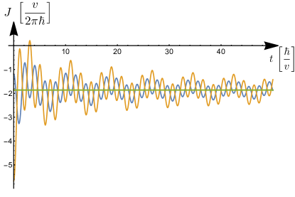
Figure 1: The inter-cell current $J^{inter}$ (blue curve) and the intra-cell current $J^{intra}$ (yellow curve) resulting from a sudden flux quench in the SSH model are plotted as a function of time. At long-time, they both tend to the same stationary contribution $J_{dc}$ (green curve). The time evolution is computed in the thermodynamic limit for $r=0.6$ and $\phi_{i}=\pi/2$.

A few comments are in order about such persistent current $J_{dc}$. First, $J_{dc}$ is essentially different from the current flowing at equilibrium in a mesoscopic ring threaded by a flux, since it is non-vanishing also in the thermodynamic limit, where it acquires the form

$$J_{dc} = {\frac{v}{2\pi\hbar}}\int_{-\pi}^{\pi}d(ka)\,\frac{r\sin(ka)}{{\epsilon(k,0)}}\times$$ (23)

$$\times\frac{(1+r^{2})\cos{\phi}_{i}+2r\cos(ka+{\phi}_{i})}{{\epsilon(k,\phi_{i})}{\epsilon(k,0)}}$$

Second, $J_{dc}$ cannot be captured by the LRT, which would predict a vanishing persistent current due to a vanishing Drude weight (see Appendix VI.3). This can also be seen by inspecting Eq.(23) in the limit of weak initial flux ${\phi}_{i}\ll 1$, which corresponds to the limit of weak applied electric pulse. Indeed one obtains

$$J_{dc}\approx-{\frac{v\,r^{2}}{\pi\hbar}}(1-r^{2})^{2}\left[\int_{-\pi}^{\pi}d(ka)\frac{\sin^{2}(ka)}{{\epsilon^{7}}(k,0)}\right]{\phi}_{i}^{3}\,\,$$ (24)

which highlights the non-linear (cubic) response of the insulating SSH ring.

It is now worth comparing the above results with the one of the non-dimerized limit $r\rightarrow 1$, where one obtains for the post-quench currents ($t>0$)

$$J^{inter}(t)=J^{intra}(t) = -{\frac{2v}{\pi\hbar}}\sin{\phi}_{i}\quad.$$ (25)

Differently from the result obtained for the dimerized case (see Fig.1), the current (25) is time-independent after the quenchfootnote and, for a weak field $\phi_{i}\ll 1$, it exhibits a linear dependence on $\phi_{i}$. One thus recovers the well known finite Drude weightfootnote_Drude $D=-(e^{2}/\hbar)\mathtt{v}_{F}/\pi$, where $\mathtt{v}_{F}$ is the Fermi velocity, of a non interacting half filled metallic band, as predicted by LRTgiamarchi_book .
The role of dimerization is emphasized in Fig.2, where the persistent current (23) is depicted as a function of the initial flux, for various values of dimerization $r$. While at small flux values $\phi_{i}\ll 1$ the current $J_{dc}$ of the dimerized case $r\neq 1$ is suppressed as compared to the metallic case $r=1$ (green curve), for finite flux values the two cases exhibit comparable currents.

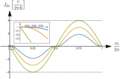
Figure 2: The persistent current $J_{dc}$ induced in the SSH model by quenching the flux to zero is plotted as a function of the initial flux $\phi_{i}$. The blue, yellow and green curves are obtained for different dimerization strengths, namely $r=(0.6,0.8,1)$ respectively. For each value of $r\neq 1$ the current does not exhibit a linear term in $\phi_{i}$ for $\phi_{i}\ll 1$. The inset magnifies the behaviour at small fluxes to highlight the difference between linear and non linear response.

The origin of the persistent current term $J_{dc}$ can be understood in terms of the out of equilibrium occupancies $n_{f,\pm}$ of the post-quench bands $\varepsilon_{\pm}(k,0)$ induced by the flux quench. These can be computed, for each $k$, by projecting the initial state on the post-quench eigenmodes, obtaining time-independent expressions

$$n_{f,\pm}(k,{\phi}_{i})=\text{tr}\left\{\rho_{i}(k)\left(\sigma_{0}\pm\mathbf{u}_{f}(k)\cdot\boldsymbol{\sigma}\right)/2\right\}$$ (26)

$$= \frac{1}{2}(1\mp\mathbf{u}_{i}(k)\cdot\mathbf{u}_{f}(k))=$$

$$= \frac{1}{2}\mp\frac{(1+r^{2})\cos{\phi}_{i}+2r\cos(ka+{\phi}_{i})}{2{\epsilon(k,{\phi}_{i})\epsilon(k,0)}}$$

which are plotted as a function of $ka/\pi$ in Fig.3. By comparing Eq.(26) with Eq.(23), the persistent current can be rewritten as

$$J_{dc}=\frac{1}{2\pi a}\int_{-\pi}^{\pi}d(ka)\,\Delta n_{f}(k,{\phi}_{i})\,\frac{1}{\hbar}\partial_{k}\varepsilon_{-}(ka)$$ (27)

where $\frac{1}{\hbar}\,\partial_{k}\varepsilon_{\pm}(k)=\pm\frac{va}{\hbar}\frac{r\sin(ka)}{\epsilon(ka)}$ are the post quench group velocities, and

$$\Delta{n}_{f}(k,{\phi}_{i}) = {n}_{f,-}(k,{\phi}_{i})-{n}_{f,+}(k,{\phi}_{i})=$$ (28)

$$= \mathbf{u}_{i}(k)\cdot\mathbf{u}_{f}(k)$$

denotes the occupancy difference. Since in Eq.(27) the group velocities are odd functions in $k$, the origin of the non-vanishing persistent current $J_{dc}$ boils down to the lack of even parity in $k$ of the post quench occupancy distributions (26) and of their difference $\Delta{n}_{f}$. Such lack of symmetry, clearly seen in Fig.3, arises from the fact that the flux quench impacts on the phase of tunneling amplitudes, whereas quenches in the magnitude of the tunneling amplitudes lead to out of equilibrium occupancy distributions that preserve their even parity in $k$ and cannot induce a net current porta_2018 .

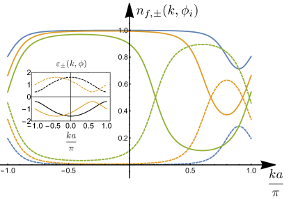
Figure 3: Occupancies of the post-quench bands for different values of the initial flux $\phi_{i}$ and a fixed dimerization strength $r=0.6$. Dashed lines correspond to the upper band, while solid lines correspond to the lower one. The blue, yellow and green colors correspond to $\phi_{i}=(0.1,0.2,0.4)\pi$, respectively. The distributions are not symmetric in $k\leftrightarrow-k$ for any value of the initial flux. As $\phi_{i}$ is increased, the upper band becomes more occupied and the lower band gets more depleted. Inset: bands $\varepsilon_{\pm}(k,\phi)$ of a SSH model pierced by a magnetic flux: Solid and dashed lines describe the lower and the upper bands, respectively. The bands are depicted for $v=1$, a fixed dimerization strength $r=0.6$ and for two different values of the flux, namely $\phi=0.2\pi$ (yellow lines) and $\phi=0$ (black lines).

We conclude this section by two comments. First, when moving away from half filling, the system becomes metallic even in the presence of dimerization. In this case one can show that the system develops a finite Drude weight and that the linear response theory well captures the quench-induced current for small initial fluxes. Nonetheless, there exist some qualitative differences with respect to the non-dimerized metallic case. Indeed, because of dimerization, the current also has a finite ac-contribution and, for small filling, it does not increase monotonically in $\phi_{i}\in[0,\pi/2]$, developing a local minimum for $\phi_{i}=\pi/2$ instead of a maximum. The second comment is concerned with the flux switching protocol. Here, in analogy to what was done in Ref.[misguich, ], we have considered the switching off of the initial flux, so that the latter only appears in the initial state. In the reversed protocol, where the flux is switched on, one obtains a current with opposite sign, as expected, provided that one consistently includes the flux phases related to the vector potential both in the post-quench Hamiltonian and in the current operators (14)-(15).

IV Dynamical Quantum Phase Transitions

Let us now analyze the properties of the Loschmidt amplitude $\mathcal{G}(t)=\langle\psi_{0}|e^{-i\hat{H}_{f}t/\hbar}|\psi_{0}\rangle$, where $|\psi_{0}\rangle$ is the many-body initial state, while $\hat{H}_{f}$ is the final Hamiltonian that governs the time evolution of the system after the quench. With applications in studies on quantum chaos and dephasing jalabert_2001 ; jarzynski_2002 ; zanardi_2006 , the Loschmidt amplitude has a tight relation to the statistics of the work performed through the quench silva_2008 ; heyl_2013 ; deluca_2014 . Equivalently, it can also be regarded as the generating function of the energy probability distribution encoded in the post quench diagonal ensemble, since $\mathcal{G}(t)=\int dEP(E)e^{-iEt/\hbar}$ and the post-quench diagonal ensemble is described by $P(E)=\sum_{n}|\langle n|\psi_{0}\rangle|^{2}\delta(E-E_{n})$, where $E_{n}$ and $|n\rangle$ are the many-body eigenvalues and eigenstates of the final Hamiltonian respectively. Moreover, it has been suggestedheyl_2013 that the Loschmidt amplitude can be interpreted as a dynamical partition function whose zeros, in analogy with the equilibrium case, are identified with DQPTs. The initial belief of a connection between DQPTs and quenches across different equilibrium phase transitions has been proved to be not rigorous dora_2014 ; andraschko_2014 ; jafari_2017 ; jafari_2019 ; budich_2020 ; jafari_2021 , and the impact of DQPTs on local observables has been found only in specific casesheyl_2013 ; fagotti_2013 ; halimeh_2017 ; halimeh_2017bis ; halimeh_2018 ; silva_2018 . Nevertheless, the existence of zeros of $\mathcal{G}(t)$ can be interpreted as a clear signature of quench-induced population inversionheyl_2013 ; defenu_2019 .

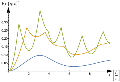
Figure 4: Time evolution of the real part of the dynamical free energy density $g(t)$, for different values of the initial flux $\phi_{i}$ at a fixed dimerization strength $r=0.6$. The blue curve corresponds to an initial flux $\phi_{i}=0.1\pi$ lying outside the range identified by Eq.(31) and is smooth. The yellow and green curves correspond to flux values that fulfill Eq.(31) ($\phi_{i}=(0.2,0.4)\pi$, respectively) and exhibit DQPT singularities.

For the present flux quench the Loschmidt amplitude explicitly readsdora_2015

$$\mathcal{G}(t) = \prod_{-\pi\leq ka\leq\pi}\left[\cos\left(\frac{{\epsilon(k,0)}vt}{\hbar}\right)\right.+$$ (29)

$$\qquad\quad\,\,\left.+i\,[\mathbf{u}_{i}(k)\cdot\mathbf{u}_{f}(k)]\sin\left(\frac{{\epsilon(k,0)}vt}{\hbar}\right)\right]$$

whence the dynamical free energy density $g(t)=-M^{-1}\log[\mathcal{G}(t)]$ in the thermodynamic limit is straightforwardly given by

$$g(t) = -\frac{1}{2\pi}\int_{-\pi}^{\pi}d(ka)\log\left[\cos\left(\frac{{\epsilon(k,0)}vt}{\hbar}\right)+\right.$$ (30)

$$\qquad\quad\,\,\left.+i[\mathbf{u}_{i}(k)\cdot\mathbf{u}_{f}(k)]\sin\left(\frac{{\epsilon(k,0)}vt}{\hbar}\right)\right]\,.\,\,$$

The argument of the logarithm in Eq.(30) may vanish at some critical times if and only if $\mathbf{u}_{i}(k)\cdot\mathbf{u}_{f}(k)=0$. Using Eqs.(28) and (26) in the regime $r\neq 1$, this condition can be satisfied by some $ka\in[-\pi,\pi]$ if and only if

$$|\cos\phi_{i}|\leq\frac{2r}{1+r^{2}}\quad.$$ (31)

In conclusion, for each value of the dimerization strength $r\neq 1$, there exists a range of initial flux values, Eq.(31), such that singularities in the dynamical free energy density appear, as shown in Fig.4. Recalling Eq.(28), we observe that DQPTs appear if and only if the post-quench band occupancies cross at some $k$, i.e. if there exists a subregion of the Brillouin zone, where the post-quench upper band is more populated then the lower one (band population inversion). This is the case for the yellow and green curves in Figs.3 and 4. Notably, while a quench across the critical point $r=1$ is sufficient to induce a DQPTdora_2015 , it is not a necessary condition and accidental DQPTs can also appeardora_2014 ; budich_2020 . This is the case here, where the DQPTs show up even if the quench is performed within the same topological phase.

Before concluding this section, a remark is in order about the specific case $r=1$, which deserves some care. At first, by looking at the limit $r\rightarrow 1$ of Eq.(31), one could naively expect that DQPTs exist for any value of the initial flux. However, this is not the case since the scalar product $\mathbf{u}_{i}(k)\cdot\mathbf{u}_{f}(k)$ reduces to a pure sign and the argument of the logarithm in Eq.(30) can never vanish. Indeed for $r=1$ the initial state is an (excited) eigenstate of the final Hamiltonian, its dynamics is trivial and $\mathcal{G}(t)$ reduces to a pure oscillating phasedeluca_2014 . Hence the Loschmidt amplitude can never vanish and the dynamical free energy density is analytic for $t>0$. Moreover, for $r=1$ a description in terms of a two band structure is redundant and a proper band population inversion can not be defined without ambiguities.

V Discussion and Conclusions

Our results have been obtained in the case of a sudden flux quench. Here we would like to briefly discuss the effects of a finite switch-off time $\tau_{sw}$. By implementing a time-dependent flux phase $\phi(t)=\phi_{i}(1-\text{Erf}(\sqrt{8}t/\tau_{sw}))$ and by numerically integrating the Liouville von-Neumann equation for the density matrix, one can show that the persistent current $J_{dc}$ depends on the ratio $\tau_{sw}/\tau_{g}$, where $\tau_{g}=\hbar/(2v|1-r|)$ is the timescale associated to the energy gap of the SSH model. In particular, while for $\tau_{sw}\ll\tau_{g}$ the persistent current $J_{dc}$ is robust, when $\tau_{sw}\simeq\tau_{g}$ it reduces with respect to the sudden quench value (e.g. to roughly $1/5$ for the parameters of Fig.1) and it vanishes in the limit $\tau_{sw}\gg\tau_{g}$ of an adiabatic switch-off. In such limit, a vanishing stationary current is consistent with the recent generalization of LRT to higher order response, which predicts that in a band insulator the response to an adiabatic electric field vanishes to all orders in the field strengthoshikawa1 ; oshikawa2 ; resta_arxiv .

It is worth pointing out the essential difference between the quench induced dynamics in an insulating and in a metallic state. For a metallic state, where the response to a weak electric pulse is linear, the persistent current that eventually flows is independent of the quench protocol and is thus fully encoded in the Drude weight. In striking contrast, when a weak field is applied to an insulating state (like the half-filled SSH model), the response is non-linear and does depend on the quench protocol. Thus, while the vanishing higher order generalized Drude weightsoshikawa1 ; oshikawa2 only capture the behavior of the system in the adiabatic switching limit, for a sufficiently fast switching a persistent current does flow even in an insulator.

In conclusion, in this paper we have analyzed the response of a half filled SSH ring to a sudden flux quench, or equivalently, to a sudden pulse of electric field. We have shown that the intrinsically spinorial nature of the problem, due to the dimerization of the hopping amplitudes, induces a non trivial current dynamics even without interactions. In particular, a time-dependent current flows along the ring and eventually reaches a stationary value, despite the insulating nature of the initial state (see Fig.1). Such persistent current $J_{dc}$, which depends cubically on a weak initial flux $\phi_{i}$ in the presence of dimerization [see Eq.(24) and Fig.2], is a clear hallmark of a non-linear dynamics and it is ascribed to the peculiar non-equilibrium occupancy induced by the quench (see Fig.3). For suitable dimerization and flux values, a post quench population inversion occurs, which in turn implies the occurrence of DQPTs (see Fig.4). Notably, the DQPTs are present even without closing the gap, i.e. when the quench is performed within the same topological phase.

VI Appendix

VI.1 State evolution in a quenched two-band system

In this appendix we recall the general state evolution after a sudden quench in a two-band modelyang_2018 . Let us suppose that the initial state is the half filled ground state of a two-band Hamiltonian, whose one-body form can be written in momentum space as

$$H_{i}(k)=v\left[d_{i}^{0}(k)\sigma_{0}+\mathbf{d}_{i}(k)\cdot\boldsymbol{\sigma}\right]$$ (32)

where $v$ denotes the reference energy scale. The $k$-th component of the initial state can thus be written as $\rho(k,0)=\big{[}\sigma_{0}-\mathbf{u}_{i}(k)\cdot\boldsymbol{\sigma}\big{]}/2$ where $\mathbf{u}_{i}(k)=\mathbf{d}_{i}(k)/|\mathbf{d}_{i}(k)|$. The state evolves according to the post-quench Hamiltonian

$$H_{f}(k)=v\left[d_{f}^{0}(k)\sigma_{0}+\mathbf{d}_{f}(k)\cdot\boldsymbol{\sigma}\right]$$ (33)

and, by solving the Liouville-Von Neumann equation for the one-body density matrix, one can write the $k$-th component of the time evolved state as $\rho(k,t)=\big{[}\sigma_{0}-\mathbf{u}(k,t)\cdot\boldsymbol{\sigma}\big{]}/2$, where the time dependent unit vector can be written as the sum of three orthogonal contributions:

$$\mathbf{u}(k,t) = \mathbf{d}_{\parallel}(k)+\mathbf{d}_{\bot}(k)\cos\big{[}2|\mathbf{d}_{f}(k)|vt/\hbar\big{]}+$$ (34)

$$\hskip 27.0pt+\mathbf{d}_{\times}(k)\sin\big{[}2|\mathbf{d}_{f}(k)|vt/\hbar\big{]}$$

where

$$\mathbf{d}_{\parallel}(k) = \Big{[}\mathbf{u}_{i}(k)\cdot\mathbf{u}_{f}(k)\Big{]}\mathbf{u}_{f}(k)$$

$$\mathbf{d}_{\bot}(k) = \Big{[}\mathbf{u}_{i}(k)-\mathbf{d}_{\parallel}(k)\Big{]}$$

$$\mathbf{d}_{\times}(k) = -\Big{[}\mathbf{u}_{i}(k)\times\mathbf{u}_{f}(k)\Big{]}$$

Then, by inserting the explicit expression for $\mathbf{d}_{i}(k)$ and $\mathbf{d}_{f}(k)$ corresponding to a flux quench in the SSH model, see Eq. (LABEL:d-vec) of the Main Text, the expressions in Eqs. (8), (9) and (10) are recovered.

VI.2 Current

In this appendix we briefly outline how to derive the current operators discussed in Sec.III. Given the site density operators $\hat{n}_{j,\alpha}=\hat{c}_{j\alpha}^{\dagger}\hat{c}_{j\alpha}$, with $\alpha=A,B$, and the SSH Hamiltonian with $\phi=0$ (see Eq.(1) of the Main Text), it is straightforward to derive the following Heisenberg equations of motion:

$$\partial_{t}\hat{n}_{jA} = {\hat{J}_{j-1}^{inter}}-{\hat{J}_{j}^{intra}}$$

$$\partial_{t}\hat{n}_{jB} = {\hat{J}_{j}^{intra}}-{\hat{J}_{j}^{inter}}$$

where, by definition:

$$\hat{J}_{j}^{inter}=\frac{rv}{\hbar}\left[i\hat{c}_{jB}^{\dagger}\hat{c}_{j+1A}-i\hat{c}_{j+1A}^{\dagger}\hat{c}_{jB}\right]$$

is the inter-cell current reported in Eq.(14), while:

$$\hat{J}_{j}^{intra}=\frac{v}{\hbar}\left[i\hat{c}_{jA}^{\dagger}\hat{c}_{jB}-i\hat{c}_{jB}^{\dagger}\hat{c}_{jA}\right]$$

is the intra-cell current reported in Eq.(15).

VI.3 Drude weight

The Drude weight $D$ characterizing the LRT of the SSH model can be computed following Kohn’s approach[kohn_1964, ]. In particular, in a 1D ring one has

$$D=-L\frac{d^{2}E_{0}(\Phi)}{d^{2}\Phi}\bigg{|}_{\Phi=0}$$

where $E_{0}(\Phi)$ denotes the dependence of the many-body ground state energy on the magnetic flux $\Phi$ threading the ring, while $L$ denotes the ring length. For a tight-binding model, we can associate the magnetic flux $\Phi$ to a phase $\phi$ in the hopping amplitudes according to $N\phi=2\pi\Phi/\Phi_{0}$, where $N$ is the number of links in the ring and $\Phi_{0}=h/e$ is the magnetic flux quantum. Hence, in a bipartite lattice with two sites per cell, we get:

$$\Phi=L\,\frac{2}{a}\,\frac{\hbar}{e}\,\phi$$ (35)

where $a$ is the lattice constant. Exploiting the linear relation between $\phi$ and $\Phi$ we can write Kohn’s formula as

$$D=-\left(\frac{a}{2}\right)^{2}\left(\frac{e}{\hbar}\right)^{2}L^{-1}\frac{d^{2}E_{0}(\phi)}{d^{2}\phi}\bigg{|}_{\phi=0}$$ (36)

Moreover, for translation invariant one-body Hamiltonians we can write:

$$D = -\left(\frac{a}{2}\right)^{2}\left(\frac{e}{\hbar}\right)^{2}L^{-1}\left[\frac{d^{2}}{d^{2}\phi}\sum_{(k,b)\in\mathcal{I}}\varepsilon_{b}(k,\phi)\right]_{\phi=0}$$

where $\mathcal{I}$ denotes the set of bands $b$ and wavevectors $k$ that are occupied in the many body ground state without flux, while $\varepsilon_{b}(k,\phi)$ denotes the band dispersion relations for a finite flux.

Since the single particle energies depend on the phase $\phi$ only through the combination $ka+2\phi$, see Eq.(4) in the Main Text, the many-body ground state energy of a half filled SSH model with dimerization ($r\neq 1$) does not depend on the flux in the thermodynamic limit. Indeed, due to the periodic nature of the lower band over the interval $ka\in[-\pi,\pi]$, one has

$$L^{-1}E_{0}^{r\neq 1}(\phi) = \frac{1}{2\pi}\frac{1}{a}\int_{-\pi}^{\pi}d(ka)\varepsilon_{-}(k,\phi)$$

$$= \frac{1}{2\pi}\frac{1}{a}\int_{-\pi}^{\pi}d(ka)\varepsilon_{-}(k,0)=L^{-1}E_{0}^{r\neq 1}(0)$$

and we conclude that the Drude weight (36) is identically zero in this case, consistently with Eq.(24) of the Main Text.

Without dimerization ($r=1$) the situation is different, since we get

$$L^{-1}E_{0}^{r=1}(\phi) = -\frac{v}{\pi}\frac{2}{a}\int_{-\frac{\pi}{2}}^{\frac{\pi}{2}}d\big{(}\frac{ka}{2}\big{)}\cos\big{(}\frac{ka}{2}+\phi\big{)}$$

$$= -\frac{2v}{\pi}\frac{2}{a}\cos(\phi)$$

and from Eq.(36) one obtains

$$D=-\frac{e^{2}}{\hbar}\frac{2v}{\hbar\pi}\frac{a}{2}=-\frac{e^{2}}{\hbar}\frac{\mathtt{v}_{F}}{\pi}$$

where $\mathtt{v}_{F}$ is the Fermi velocity. The finite Drude weight computed in this way coincides with the one obtained in the Main Text (see Eq.(25)) through its dynamical definition.

References

- (1) R. Kubo, J. Phys. Soc. Jpn. 12, 570 (1957).
- (2) G. D. Mahan, Many Particle Physics, Springer, Boston, 3rd Edition (2000)
- (3) R. Resta, J. Phys.: Condens. Matter 30, 414001 (2018)
- (4) W. Kohn, Phys. Rev. 133, A171 (1964).
- (5) B.S. Shastry and B. Sutherland, Phys. Rev. Lett. 65, 243 (1990)
- (6) N. Kawakami and S.-K. Yang, Phys. Rev. B 44, 7844 (1991)
- (7) H. Castella, X. Zotos, and P. Prelovsek, Phys. Rev. Lett. 74, 972 (1995)
- (8) Zotos, Phys. Rev. Lett. 82, 1764 (1999).
- (9) J. Benz, T. Fukui, A. Klümper, and C. Scheeren, J. Phys. Soc. Jpn 74, 181 (2005)
- (10) J. Herbrych, P. Prelovšek, and X. Zotos, Phys. Rev. B 84, 155125 (2011)
- (11) C. Karrasch, J. H. Bardarson, and J. E. Moore, Phys. Rev. Lett. 108, 227206 (2012)
- (12) M. Mierzejewski, P. Prelovšek, and T. Prosen, Phys. Rev. Lett. 113, 020602 (2014)
- (13) C. Karrasch, T. Prosen, and F. Heidrich-Meisner, Phys. Rev. B 95, 060406(R) (2017)
- (14) D. Rossini, R. Fazio, V. Giovannetti, and A. Silva, Eur. Phys. Lett. 107, 30002 (2014)
- (15) M. Lewenstein, A. Sanpera, V. Ahufinger, B. Damski, A. Sen, and U. Sen, Adv. Phys. 56, 243 (2007)
- (16) I. Bloch, J. Dalibard, and W. Zwerger, Rev. Mod. Phys. 80, 885 (2008)
- (17) J. Dalibard, F. Gerbier, G. Juzeliunas, and P. Öhberg, Rev. Mod. Phys. 83, 1523 (2011)
- (18) N. Goldman, G. Juzeliunas, P. Öhberg, and I. B. Spielman, Rep. Prog. Phys. 77, 126401 (2014)
- (19) P. Calabrese, and J. Cardy Phys. Rev. Lett. 96, 136801 (2006)
- (20) A. Polkovnikov, K. Sengupta, A. Silva, and M. Vengalattore, Rev. Mod. Phys. 83, 863 (2011)
- (21) J. Eisert, M. Friesdorf, C. Gogolin, Nat. Phys. 11 124 (2015)
- (22) A. Mitra, Ann. Rev. Cond. Mat. Phys. 9 245 (2018)
- (23) Y.O. Nakagawa, G. Misguich, M. Oshikawa, Phys. Rev. B 93, 174310 (2016)
- (24) W.P. Su, J.R. Schrieffer, and A.J. Heeger, Phys. Rev. Lett. 42 1698 (1979)
- (25) W.P. Su, J.R. Schrieffer, and A.J. Heeger, Phys. Rev. B 22 2099 (1980)
- (26) M. Atala, M. Aidelsburger, J.T. Barreiro, D. Abanin, T. Kitagawa, E. Demler, I. Bloch, Nat. Phys. 9, 795-800 (2013)
- (27) E.J. Meier, F.A. An, and B. Gadway, Nat. Commun. 7 13986 (2016)
- (28) D. Xie, W. Gou, T. Xiao, B. Gadway, and B. Yan, npj Quantum Inform. 5 55 (2019)
- (29) J. K. Asbóth, L. Oroszlány, and A. Pályi, A short course on topological Insulators, Springer, Berlin (2016)
- (30) C.-Q. Shen, Topological Insulators, Springer, Heidelberg (2012)
- (31) M. Heyl, A. Polkovnikov, and S. Kehrein, Phys. Rev. Lett 110 135704 (2013)
- (32) S. Vajna, B. Dora, Phys. Rev. B 91, 155127 (2015)
- (33) R. E. Peierls, Z. Phys. 80, 763 (1933)
- (34) M. Graf, and P. Vogl, Phys. Rev. B 51, 4940 (1995)
- (35) C. Yang, L. Li, and S. Chen, Phys. Rev. B 97, 060304(R) (2018)
- (36) The non-dimerized limit acquires a time dependent current only in the presence of interactions, see Ref.[misguich, ].
- (37) The expression for is obtained by re-expressing the phase in terms of the the initial magnetic flux (see Eq.(35) in Appendix VI.3). Moreover an additional factor has to be included to obtain the charge current from the particle current in Eq.(25).
- (38) T. Giamarchi, Quantum Physics in one-dimension, Clarendon Press, Oxford (2003)
- (39) S. Porta, N.T. Ziani, D.M. Kennes, F.M. Gambetta, M. Sassetti, and F. Cavaliere, Phys. Rev. B 98, 214306 (2018)
- (40) R.A. Jalabert and H. M. Pastawski, Phys. Rev. Lett. 86, 2490 (2001)
- (41) Z.P. Karkuszewski, C. Jarzynski, and W. H. Zurek, Phys. Rev. Lett. 89, 170405 (2002)
- (42) H.T. Quan, Z. Song, X.F. Liu, P. Zanardi, and C.P. Sun, Phys. Rev. Lett. 96, 140604 (2006)
- (43) A. Silva, Phys. Rev. Lett. 101 120603 (2008)
- (44) A. De Luca, Phys. Rev. B 90, 081403(R) (2014)
- (45) S. Vajna, and B. Dora, Phys. Rev. B 89 161105(R) (2014)
- (46) F. Andraschko, and J. Sirker, Phys. Rev. B 89 125120 (2014)
- (47) R. Jafari, and H. Johannesson, Phys. Rev. Lett. 118 015701 (2017)
- (48) R. Jafari, H. Johannesson, A. Langari, and M. A. Martin-Delgado, Phys. Rev. B 99, 054302 (2019)
- (49) L. Pastori, S. Barbarino, and J.C. Budich, Phys. Rev. Research 2 033259 (2020)
- (50) M. Sadrzadeh, R. Jafari, and A. Langari, Phys. Rev. B 103, 144305 (2021)
- (51) M. Fagotti, arxiv:1308.0277 (2013)
- (52) J. C. Halimeh, and V. Zauner-Stauber, Phys. Rev. B 96, 134427 (2017)
- (53) I. Homrighausen, N. O. Abeling, V. Zauner-Stauber, and J. C. Halimeh, Phys. Rev. B 96, 104436 (2017)
- (54) J. Lang, B. Frank, and J. C. Halimeh, Phys. Rev. B 97, 174401 (2018)
- (55) B. Zunkovic, M. Heyl, M. Knap, and A. Silva, Phys. Rev. Lett. 120, 130601 (2018)
- (56) N. Defenu, T. Enss, and J. C. Halimeh, Phys. Rev. B 100, 014434 (2019)
- (57) H. Watanabe, and M. Oshikawa, Phys. Rev. B 102, 165137 (2020)
- (58) H. Watanabe, Y. Liu, and M. Oshikawa, J. Stat. Phys. 181, 2050 (2020)
- (59) R. Resta, arXiv:2111.12617 (2021)