Neural Networks with Divisive normalization
for image segmentation with application in cityscapes dataset

Abstract

One of the key problems in computer vision is adaptation: models are too rigid to follow the variability of the inputs. The canonical computation that explains adaptation in sensory neuroscience is divisive normalization, and it has appealing effects on image manifolds. In this work we show that including divisive normalization in current deep networks makes them more invariant to non-informative changes in the images. In particular, we focus on U-Net architectures for image segmentation. Experiments show that the inclusion of divisive normalization in the U-Net architecture leads to better segmentation results with respect to conventional U-Net. The gain increases steadily when dealing with images acquired in bad weather conditions. In addition to the results on the Cityscapes and Foggy Cityscapes datasets, we explain these advantages through visualization of the responses: the equalization induced by the divisive normalization leads to more invariant features to local changes in contrast and illumination.

Keywords— Divisive normalization, Adaptation, Manifold alignment, Image segmentation, Neural networks.

1 Introduction

A fundamental problem in image analysis is the variability of the image manifold depending on acquisition conditions [1]. Usually sources are not stationary: the texture and color of an object can be different depending on the acquisition conditions (see Fig. 1). This has an obvious negative impact on applications such as segmentation. Adaptation to (and compensation of) non-informative factors of variation is key for optimal segmentation. However it is not clear how deep-learning, e.g. the popular U-Nets [2], actually achieve this.

In this work we propose the use of the canonical computation that accounts for adaptation in biological neurons, namely divisive normalization [3], to improve adaptation of artificial networks in an explainable way. We illustrate this adaptation ability in image segmentation under different atmospheric conditions.

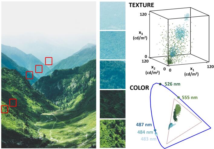
Figure 1: The problem: changes along the image due to non-informative factors. In this example, texture and color locally change due to the shadows, illumination, atmospheric scattering and depth (see highlighted regions). Associated problems for statistical learning are shown in the scatter plots (where samples are colored according to their region). The top-right plot shows changes in the spatial texture defined by the luminance of neighbor pixels: the contrast (distance from the diagonal) is smaller for lighter regions (away from the origin), and the energy in the different directions of the image space (spatial frequency) locally changes along the image. Atmospheric scattering implies local changes in the hue: see the shift in dominant wavelengths in the CIExy color diagram.

2 Why Using Divisive normalization?

The linear+nonlinear structure of conventional artificial neurons [4] comes from the seminal computation proposed for sensory neurons [5]: $\mathbf{x}\overset{\mathcal{L}}{\longrightarrow}\mathbf{z}\overset{\mathcal{N}}{\longrightarrow}\mathbf{y}$, where the intermediate linear response, $\mathbf{z}=\mathcal{L}\cdot\mathbf{x}$, is given by the matrix $\mathcal{L}$, that contains the so called (linear) receptive fields, and original versions of $\mathcal{N}(\cdot)$ were simple point-wise threshold or saturating functions [6] eventually rectified. These were the inspiration for current sigmoids/ReLU in deep-learning [4].

In sensory neuroscience, the divisive normalization model of $\mathcal{N}(\cdot)$ was a way to account for the inhibitory effect of neighbor neurons within a layer [3]:

$$y_{ip} = \frac{z_{ip}}{\left(\beta_{i}+\sum_{jp^{\prime}}{\gamma_{ijpp^{\prime}}|z_{jp^{\prime}}|^{\alpha_{j}}}\right)^{\epsilon_{i}}}$$ (1)

where the linear response of a neuron tuned to the $i$-th feature and to the $p$-th spatial location, $z_{ip}$, is inhibited (normalized) by a pool of the activity of neighbor neurons tuned to other features and spatial locations $z_{jp^{\prime}}$. The constant $\beta_{i}$ determines the level in which the pool generates effective inhibition, and the exponents control the norm of the pool. While the interaction kernel in the denominator, $\gamma$, can have whatever dense structure [7], in visual neuroscience the spatial interaction is usually assumed to be convolutional in the fovea [8].

However, why using this biological transform to improve artificial networks devoted to image segmentation? There are examples of the effectiveness of divisive normalization in many applications as image coding [9, 10, 11], restoration [12, 13], distortion metrics [14, 15, 16], classification [17, 18, 19, 20] or even referring to its appealing statistical properties [21, 22, 23, 24, 25]. Here we illustrate the effect of divisive normalization with an explicit example. Fig. 2 considers a patch from the forest (from Fig. 1) that displays a space varying contrast due to atmospheric effects, and shows how divisive normalization modifies the features and the image manifold in a positive way to identify this object class.

The spatial texture problem is enough to stress the point of local normalization so in this motivating example we restrict ourselves to the luminance channel. In this achromatic context, a reasonable physiological model of texture perception includes a linear layer of wavelet-like filters (in this illustration $\mathcal{L}$ is a steerable wavelet transform as in [21, 7]), and a divisive normalization (in this case with the psychophysically tuned parameters in [28]).

The neighborhood in $\gamma$ that defines the pooling region (illustrated in Fig. 2 by the circles in the feature vectors or wavelet bands) has a qualitatively relevant effect: the division by the local pool moderates the response in regions where contrast is high, in orange, while boosts the response in regions of low contrast, in white. See the difference between the features before and after the local normalization, and note the equalization of the amplitude of the edges along the field of view. The local normalization compensates for the contrast variation along the image due to atmospheric conditions. As a result, while the distribution of the samples from the original luminance channel display separate clusters corresponding to spatial variations of the texture, the different samples have been compacted due to the contrast equalization effect.

In the discussion we will explicitly check if the artificial networks for segmentation equiped with divisive normalization also develop this contrast enhancement and equalization effects that have been found in biological neurons.

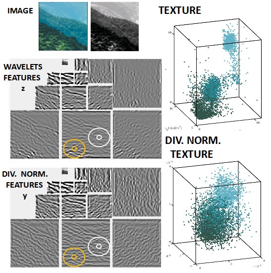
Figure 2: The idea for the solution: manifold equalization though Divisive Normalization. At the top-left we have the luminance input to a linear+nonlinear model of the V1 cortex based on wavelets and divisive normalization [21, 7, 28]. Below we have the wavelet-like linear features, $\mathbf{z}=\mathcal{L}\cdot\mathbf{x}$, and the corresponding divisive normalized features, $\mathbf{y}=\mathcal{N}(\mathbf{z})$. The scatter plots display the distributions of image patches taken from $\mathbf{x}$ and $\mathbf{x^{\prime}}$.

3 Models and Experiments

In order to confirm the intuition obtained from the 1-layer, purely biological, non-optimized model presented in the previous section, here we implemented the generic divisive normalization layer in Eq. 1 in an automatic differentiation context. Therefore, one may include our layer at any place of any architecture and optimize the network for the desired task.

Qualitatively critical points are (a) the nature of the interaction kernel, $\gamma$, and (b) the specific locations to include the normalization in the U-Nets for segmentation.

Regarding the nature of $\gamma$, the above example points out that the consideration of spatial neighborhoods is convenient to get the local contrast equalization along the visual field required to overcome shadow, scattering or fog. The recent literature that exploits automatic differentiation shows a range of kernel structures: some do not consider spatial interactions (either in a dense [24, 11, 16] or convolutional [20] combinations of features); while others do with some restrictions (either uniform weights [29], a ring of locations [18, 19], or special symmetries in the space [30]). Following biology [8, 21, 3, 28] and the intuition pointed out in the previous section. In our experiments we use the version in Eq. 1 which includes a general spatial surround, as in [29], but allowing variable weights over space. Additionally a general (dense) interaction over channels was considered. Besides the $\gamma$ parameter, the $\beta$ parameter is also trained, but we set $\alpha$ and $\epsilon$ to $1$ which we found it makes the training more stable.

Regarding where to include the proposed normalization in U-Nets, we recall the color and texture problems pointed out in Fig. 1: following color appearance models [26, 27], constancy maybe addressed by a single normalization of the photoreceptors (right before the first convolution), while texture equalization over space may require normalization at deeper stages where filters tuned to specific patterns have emerged. This intuition lead us to the specific scheme in Fig. 3 where green layers stand for the proposed divisive normalization. Note that we propose modifications only in the encoding/compressive part, where the features that will lead to the segmentation are computed. The color/texture distinction shapes the experiments because we will compare the behavior of the improved network (4 DN layers) with regard to the No-DN network, but we will also consider a 1 DN layer network eventually addressing only the color problem, but not the texture problem.

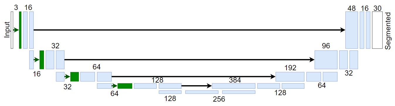
Figure 3: U-Net for segmentation including 4 DN layers (in green). Black arrows represent the skip unions. The model with only one DN layer had only the first green layer. The model without DN layers did not have any of the green layers. The consideration of the DN layers only increases the number of parameters by an 1.8$\%$.

In the experiments we used the Cityscapes dataset [31], that includes scenes with annotated segmentation ground truth and the Foggy Cityscapes dataset [32], that includes degraded versions of the scenes simulating poor weather conditions of controlled (low, medium, high) severity. In fog, spatial varying degradation is a major problem. The bottom pixels of each image were cropped from $1024\times 2048$ to $768\times 2048$ and then normalized and resized to $96\times 256$ to maintain the aspect ratio. We used 2675, 300 and 500 images for train, validate and test. We used MAE loss function, a batch-size of 64 and Adam optimiser with an initial learning rate of $0.001$ during 500 epochs with the original scenes (in regular weather conditions). We kept the models with higher Intersection over Union (IoU) in validation (in regular weather) and used these for the test (in poor weather). Testing in more general datasets where visibility is strongly reduced will confirm or refute the intuition in Fig. 2.

4 Results and Discussion

Dataset	No DN	1 DN	4 DN
Original	0.73	0.73 (0.0%)	0.78 (6.8%)
Low fog	0.65	0.63 (-3.1%)	0.70 (7.7%)
Middle fog	0.55	0.52 (-5.5%)	0.61 (10.9%)
High fog	0.39	0.42 (7.7%)	0.46 (17.9%)

IoU reductions (due to fog)
Dataset change	No DN	1 DN	4 DN
Original-low fog	-11.0%	-14.3%	-9.8%
Original-middle fog	-24.9%	-28.8%	-21.9%
Original-high fog	-46.9%	-42.6%	-40.9%

Table 1: Top: IoU performance in test. Improvements of the use of DN layers with regard no using DN in parenthesis. Bottom: Reductions in test IoU when comparing each fog level with the original.

The top panel in Table 1 shows the test results of each model in the four weather conditions for models trained only using the original (good weather conditions) images. The bottom panel shows how the test IoU changes in poor conditions with regard to regular weather.

The first observation is that using 4-DN layers gives substantial increase in IoU in all cases. Using just 1-DN only helps in really heavy fog. This is consistent with the previous explanation since introducing fog into the images mainly changes the textures, which as previously mentioned requires several normalizations in deep stages. Second, as expected, for progressively heavier fog, IoU gets reduced in all cases. However the conventional architecture is more sensitive to the decrease in visibility (bigger reductions in performance) than the architecture with 4-DN layers. And third, the use of 4-DN always leads to improvements with regard the no-DN case, but it is important to see that the gains get progressively bigger when the acquisition conditions are poor.

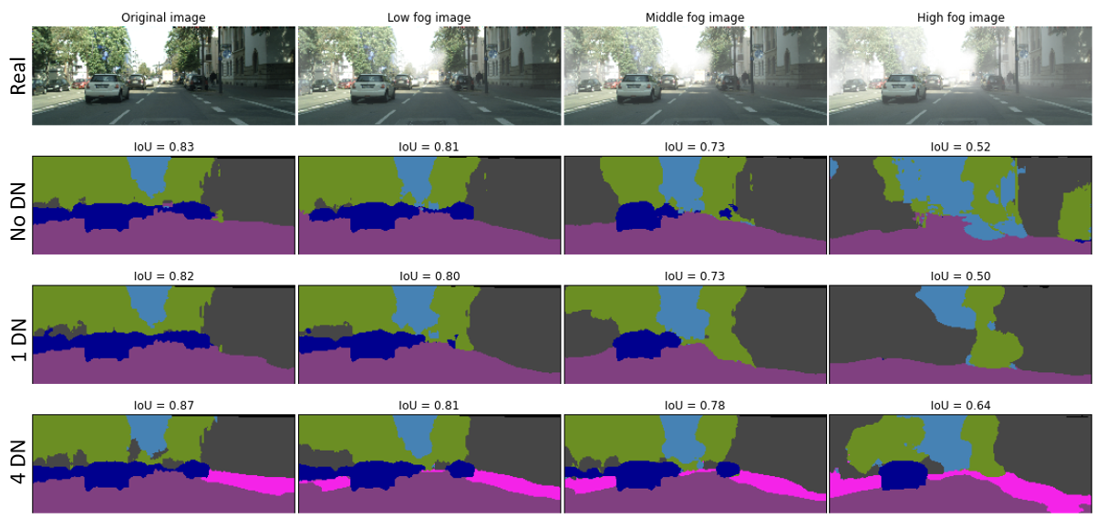
Figure 4: Segmentation results for the four datasets (original, low, middle and high fog) and the three models.

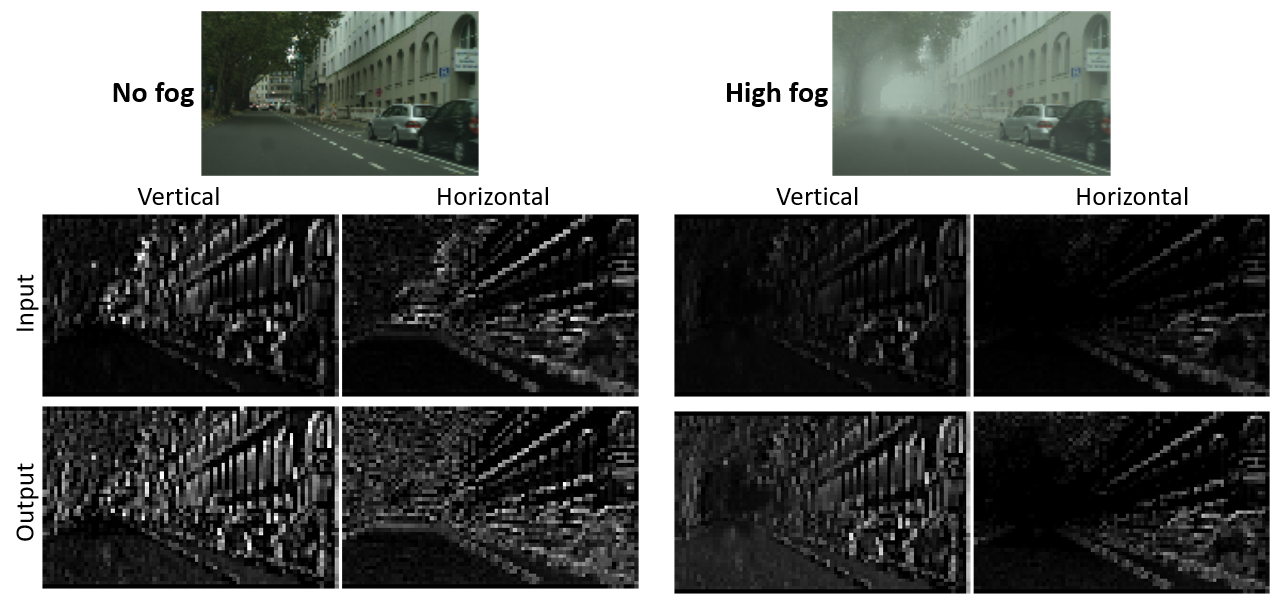
Figure 5: Effect of the 2nd-DN layer in two channels, one tuned to vertical and one tuned to horizontal features: activity before (input) and after (output) the divisive normalization layer. Results are shown for two different fog situations.

Figure 4 shows illustrative examples of the predictions, which are consistent with average IoUs in the tables. Note that only the 4-DN model is able to get the border in the shadow and preserve the detection of the car in heavy fog.

In order to understand the above advantages we explored the effect of the two initial DN layers. The first DN, applied to the input RGB signal performs a Weber-like saturating non-linearity (not shown), very much like a square root equalization in the separate channels: it boosts low values and moderates high values. More interestingly, Fig. 5 shows the effect of the second DN layer on two illustrative features tuned to horizontal and vertical edges (key for object recognition). We see that in the foggy image the deepest parts of the image were impossible to distinguish. However, after applying the DN transformation that the model had learnt with the original (no foggy) images, the output is much more like the case without fog, now being able to distinguish details that are further away.

5 Conclusion

We presented results in image segmentation when including divisive normalization in the U-Net architecture. We found that introducing more than one divisive normalization layer leads us to an improvement in IoU in the Cistyscapes dataset. Moreover, a model trained only with images acquired in good weather conditions obtains an increase in IoU over conventional U-Net when tested with images in bad weather conditions. In fact, the higher the level of fog introduced in the images, the higher the advantage, which shows that this transformation helps the models to be more invariant under the non-informative variations introduced by contrast and luminance changes.

References

- [1] Y. Bengio, “Learning deep architectures for AI,” Fdns and Trends in ML, vol. 2, no. 1, pp. 1–127, 2009.
- [2] O. Ronneberger et al., “U-net: Convolutional networks for biomedical image segmentation,” in 2015 MICCAI, 2015, pp. 234–241.
- [3] M. Carandini et al., “Normalization as a canonical neural computation,” Nature Reviews Neuroscience, vol. 13, pp. 51–62, 2012.
- [4] S.S. Haykin, Neural networks and learning machines, Pearson Education, Upper Saddle River, NJ, third edition, 2009.
- [5] D. H. Hubel et al., “Receptive fields of single neurons in the cat’s striate cortex,” The Journal of Physiology, vol. 148, no. 3, pp. 574–591, 1959.
- [6] K. I. Naka et al., “S‐potentials from luminosity units in the retina of fish (cyprinidae),” The Journal of Physiology, vol. 185, no. 3, pp. 587–599, 1966.
- [7] M. Martinez-Garcia et al., “Derivatives and inverse of cascaded linear+ nonlinear neural models,” PloS One, vol. 13, no. 10, pp. e0201326, 2018.
- [8] A. Watson et al., “Model of visual contrast gain control and pattern masking,” JOSA, vol. 14, no. 9, pp. 2379–2391, 1997.
- [9] I. Epifanio et al., “Linear transform for simultaneous diagonalization of covariance and perceptual metric matrix in image coding,” Pattern Recognition, vol. 36, pp. 1799–1811, 08 2003.
- [10] J. Malo et al., “Nonlinear image representation for efficient perceptual coding,” TIP, vol. 15, pp. 68–80, 2006.
- [11] J. Ballé et al., “End-to-end optimized image compression,” in 2017 ICLR. 2017, OpenReview.net.
- [12] J. Gutiérrez et al., “Regularization operators for natural images based on nonlinear perception models,” TIP, vol. 15, no. 1, pp. 189–200, 2005.
- [13] V. Laparra et al., “Perceptually optimized image rendering,” JOSA, vol. 34, no. 9, pp. 1511–1525, Sep 2017.
- [14] A.M. Pons et al., “Image quality metric based on multidimensional contrast perception models,” Displays, vol. 20, no. 2, pp. 93–110, 1999.
- [15] V. Laparra et al., “Divisive normalization image quality metric revisited,” JOSA, vol. 27, no. 4, pp. 852–864, Apr 2010.
- [16] A. Hepburn et al., “Perceptnet: A human visual system inspired neural network for estimating perceptual distance,” in 2020 ICIP. IEEE, 2020, pp. 121–125.
- [17] R. Coen-Cagli et al., “The impact on midlevel vision of statistically optimal divisive normalization in V1,” Journal of vision, vol. 13, no. 8, pp. 13–13, 2013.
- [18] L.G. Giraldo et al., “Integrating flexible normalization into midlevel representations of deep convolutional neural networks,” Neural Computation, vol. 31, pp. 2138–2176, 2019.
- [19] X. Pan et al., “Brain-inspired weighted normalization for CNN image classification,” bioRxiv, 2021.
- [20] M. Michelle et al., “Divisive feature normalization improves image recognition performance in alexnet,” in 2022 ICLR, 2022.
- [21] O. Schwartz et al., “Natural signal statistics and sensory gain control,” Nature Neuroscience, vol. 4, no. 8, pp. 819–825, 2001.
- [22] J. Malo et al., “V1 non-linear properties emerge from local-to-global non-linear ICA,” Network: Computation in Neural Systems, vol. 17, no. 1, pp. 85–102, 2006.
- [23] J. Malo et al., “Psychophysically tuned divisive normalization approximately factorizes the pdf of natural images,” Neural Computation, vol. 22, no. 12, pp. 3179–3206, 2010.
- [24] J. Ballé et al., “Density modeling of images using a generalized normalization transformation,” in 2016 ICLR, 2016.
- [25] J. Malo, “Spatio-chromatic information available from different neural layers via gaussianization,” J. Math. Neurosci., vol. 10, no. 1, pp. 1–40, 2020.
- [26] J.M. Hillis et al., “Do common mechanisms of adaptation mediate color discrimination and appearance? uniform backgrounds,” JOSA, vol. 22, no. 10, pp. 2090–2106, 2005.
- [27] M.D. Fairchild, Color Appearance Models, IS and T Wiley Series. Wiley, Sussex, UK, 2013.
- [28] M. Martinez-Garcia et al., “In praise of artifice reloaded: Caution with natural image databases in modeling vision,” Frontiers in Neuroscience, vol. 13, 2019.
- [29] M. Ren et al., “Normalizing the normalizers: Comparing and extending network normalization schemes,” 2017.
- [30] M.F. Burg et al., “Learning divisive normalization in primary visual cortex,” PLOS Computational Biology, vol. 17, no. 6, pp. e1009028, 2021.
- [31] M. Cordts et al., “The cityscapes dataset for semantic urban scene understanding,” in 2016 CVPR, 2016.
- [32] C. Sakaridis et al., “Semantic foggy scene understanding with synthetic data,” Int. J. Comput. Vis., vol. 126, no. 9, pp. 973–992, 2018.