MD-SLAM: Multi-cue Direct SLAM

Abstract

Simultaneous Localization and Mapping (SLAM) systems are fundamental building blocks for any autonomous robot navigating in unknown environments. The SLAM implementation heavily depends on the sensor modality employed on the mobile platform. For this reason, assumptions on the scene’s structure are often made to maximize estimation accuracy. This paper presents a novel direct 3D SLAM pipeline that works independently for RGB-D and LiDAR sensors. Building upon prior work on multi-cue photometric frame-to-frame alignment [4], our proposed approach provides an easy-to-extend and generic SLAM system. Our pipeline requires only minor adaptations within the projection model to handle different sensor modalities. We couple a position tracking system with an appearance-based relocalization mechanism that handles large loop closures. Loop closures are validated by the same direct registration algorithm used for odometry estimation. We present comparative experiments with state-of-the-art approaches on publicly available benchmarks using RGB-D cameras and 3D LiDARs. Our system performs well in heterogeneous datasets compared to other sensor-specific methods while making no assumptions about the environment. Finally, we release an open-source C++ implementation of our system.

I Introduction

SLAM is a popular field in robotics, and after roughly three decades of research, effective solutions are available. As many sectors rely on SLAM, such as autonomous driving, augmented reality and space exploration, it still receives much attention in academia and industry. The advent of robust machine learning systems allowed the community to enhance purely geometric maps with semantic information or replace hard-coded heuristics with data-driven ones. Within the computer vision community, we have seen photometric (or direct) approaches used to tackle the SLAM (or Structure from Motion) problem. The direct techniques address pairwise registration by minimizing the pixel-wise error between image pairs. By not relying on specific features and having the potential of operating at subpixel resolution on the entire image, direct approaches do not require explicit data association and offer the possibility to boost registration accuracy [25]. Whereas these methods have been successfully used on monocular, stereo, or RGB-D  images, their use on 3D LiDAR data is less prominent—probably due to the comparably limited vertical resolution relation to cameras. Della Corte et al. [4] presented a multi-cue photometric registration methodology for RGB-D cameras. It is a system that extends photometric approaches to different projective models and enhances the robustness by considering additional cues such as normals and depth or range in the cost function. Recently released 3D LiDARs sensors offer up to 128 beams, making direct approaches also more attractive for LiDAR data. In addition, most LiDARs provide intensity or reflectivity information besides range data. This intensity can be used to sense a light reflectivity cue from the objects in the environment. Being able to assemble an intensity-like image out of a LiDAR scan has unleashed the possibility of using well-known computer vision appearance-based methods for place recognition [7].

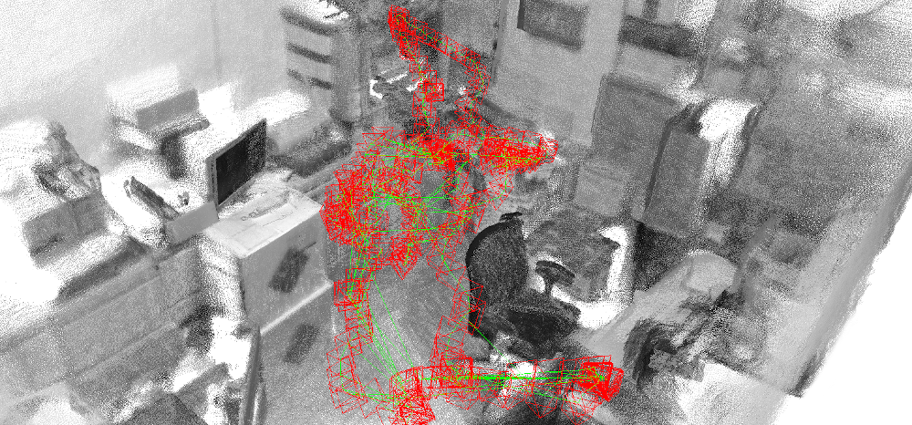
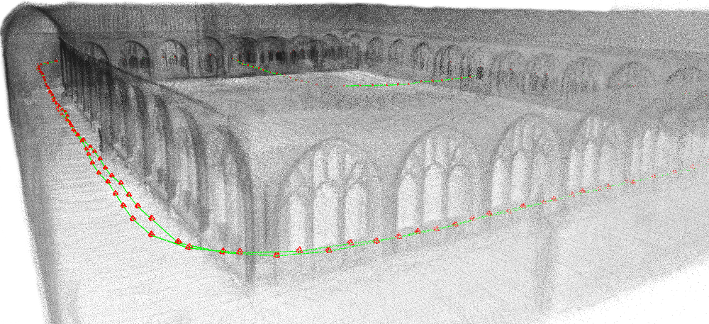
Figure 1: Scenes reconstructed using our pipeline. Top: results of a self-recorded dataset using Intel Realsense 455 RGB-D. Bottom: using LiDAR OS0-128 of the cloister sequence from the Newer College Dataset [35].

The dominant paradigm for modern SLAM systems today is graph-based SLAM. A graph-based SLAM system works by constructing a SLAM graph where each node represents the sensor position or a landmark, while edges encode a relative displacement between nodes. Pose-graphs are a particular case in which only poses are stored in the graph. These local transformations stored in the edges are commonly inferred by comparing and matching sensor readings. This paper investigates the fusion of multi-cue direct registration with graph-based SLAM.

The main contribution of this paper is a flexible, direct SLAM pipeline for 3D data. To the best of our knowledge, our approach is the only open-source SLAM system that can deal with RGB-D and LiDAR in a unified manner. We realized a revised version of MPR [4] for computing the incremental motion of the sensor operating on RGB-D as well as LiDAR data. We detect loop closures by an appearance-based algorithm that uses a Binary Search Tree (BST) structure proposed by Schlegel et al. [24], populated with binary feature descriptors [23]. All components that require the solution of an optimization problem rely on the same framework [8], resulting in a compact implementation. It is designed for flexibility, hence not optimizing the SLAM system to a specific sensor. Our system has been tested on both, RGB-D and LiDAR data, using benchmark datasets. The accuracy is competitive concerning other sensor-specific SLAM systems, while it outperforms them if some assumptions about the structure of the environment are violated. An open-source C++ implementation complements this work . Fig. 1 illustrates example maps map built with our system using RGB-D (top) and LiDAR (bottom).

II Related Work

3D SLAM has been widely addressed by the computer vision and robotics community and a large number of valid SLAM systems are available. Whereas many deserve mention, we can focus only on some seminal works due to limited space in this section. The available computational resources limited early approaches to operate offline [20] in fairly limited environments[32]. After the Kinect sensor became available about 15 years ago, we observed a revamped interest in RGB-D SLAM. Newcombe et al. [13] were the first to leverage a dense tracking on a Truncated Signed Distance Function (TSDF) stored in the GPU while using massively parallel implementation to render the surface of the local scene perceived by the sensor. Meanwhile, Segal et al [26] proposed a robust variant of Iterative Corresponding Point (ICP) relying on a point-to-plane metric. These initial methods addressed the open-loop registration approaches, tracking the pose of the sensor in a small neighbourhood. The advent of efficient optimization systems such as iSAM [15] and g2o [9], made it possible to build an effective full-fledged 3D SLAM system supporting loop closures and providing an online globally consistent estimate. Novel efficient salient floating point [1] and binary image descriptors [23], paired with bag-of-words retrieval methods inspired from web search engines, lead to impressive place recognition approaches [6]. These methods were then employed within visual SLAM systems, ORB-SLAM by Mur Artal et. al [19] being one of the most popular ones. The pipeline fully relied on the stability of features (keypoints), minimizing the reprojection error of the reconstructed landmarks within the image. In contrast to these indirect methods, another line of research aimed at photometric error minimization. Keller et al. [16] use projective data matching in a dense model, relying on a surfel-based map for tracking. Others rely on keyframe-based technique [17]. As it happened for feature-based approaches, these works were assembled into full visual SLAM systems [5]. More recently, BAD-SLAM, a surfel-based direct Bundle Adjustement (BA) system that combines photometric and geometric error [25] using feature-based loop closures, shows that, for well-calibrated data, dense BA outperforms sparse BA. The accuracy and elegance shown by photometric approaches lead to further developments such as MPR [4] aiming at unifying both LiDAR and RGB-D devices into a unique registration method.

In parallel, the community approached LiDAR-based odometry by seeking alternative representations for the dense 3D point clouds. These include 3D salient features [33, 14], subsampled clouds [30] or Normal Distributed Transform (NDT) [28]. Nowadays, LiDAR Odometry and Mapping (LOAM) is perhaps one of the most popular methods for LiDAR odometry [33, 34]. It extracts distinct features corresponding to surfaces and corners, then used to determine point-to-plane and point-to-line distances to a voxel grid-based map representation. A ground optimized version (Lego-LOAM) method has been later proposed [27], as it leverages the presence of a ground plane in its segmentation and optimization steps. In contrast to sparse methods, dense approaches suffer less in a non-structured environment [2]. Compared to RGB-D images, 3D LiDARs offer lower support for appearance-based place recognition. It is common for dense LiDAR SLAM systems to attempt a brute force registration with all neighbourhood clouds to seek loop closures. Thanks to the typically small drift, this strategy is most successful; however, computational costs grow significantly in large environments. LiDAR loop closures have been addressed in different ways compared to RGB-D. Magnusson et al. proposed an approach suitable for NDT representations [18]. Röhling et al. [22] investigated the use of histograms computed directly from the 3D point cloud to define a measure of the similarity of two scans. Novel types of descriptors have been investigated, exploiting additional data gathered by the LiDAR sensor – i.e., light emission of the beams [3, 10]. However, despite being very attractive, these descriptors are time-consuming to extract and match, resulting in a slower system overall. Recent works address loop-closures detection in a RGB-D fashion, relying on the visual feature matching extracted from the image obtained by using the LiDAR intensity channel [7].

Building on top of prior work [4, 7], this paper presents a flexible and general SLAM approach. It is a direct method working on RGB-Dand 3D LiDARdata alike providing a unified approach. Our results show that it is competitive with other sensor-specific systems.

Figure 2: Illustration of our system. Range $\mathcal{I}_{t}^{\mathrm{\rho}}$ and $\mathcal{I}_{t}^{\mathrm{i}}$ images are taken as input from the system. An optimized trajectory within a map is produced as output. This system works independently both for RGB-D and LiDAR.

III Basics

In this section, we outline some basic concepts used in multiple modules of our system. The incremental position tracking (Sec. IV-C), loop closure validation (Sec. IV-D), and pose-graph solution (Sec. IV-E) build upon Iterative Least-Squares (ILS). All these modules are built on top of the same software framework [8]. Our system generalizes on range sensors by supporting different projective models. In the remainder, we shortly describe how an ILS solution can be found and recall projective models for RGB-D and LiDARs.

III-A Iterative Optimization

A generic Least Squares problem is captured by the following equation

$$\mathbf{x}^{*}=\operatorname*{argmin}_{\mathbf{x}}\sum_{k}\|\mathbf{e}_{k}(\mathbf{x}_{k})\|_{\mathbf{\Omega}_{k}}^{2}.$$ (1)

Here $\mathbf{e}_{k}(\mathbf{x}_{k})$ is the error of the $k^{\mathrm{th}}$ measurement, which is only influenced by a subset $\mathbf{x}_{k}\in\mathbf{x}$ of the overall state vector $\mathbf{x}$ and $\|\cdot\|^{2}_{\mathbf{\Omega}}$ represents the squared Mahalonobis distance. ILS solves the above problem by refining a current solution $\mathbf{x}^{*}$. At each iteration they construct a local quadratic approximation of Eq. (1):

$$\sum_{k}\|\mathbf{e}_{k}(\mathbf{x}^{*}_{k}+\mathbf{\Delta x}_{k})\|_{\mathbf{\Omega}_{k}}^{2}\simeq\mathbf{\Delta x}^{T}\mathbf{H}\mathbf{\Delta x}+2\mathbf{b}^{T}\mathbf{\Delta x}+c.$$ (2)

The quadratic form is obtained by locally linearizing the vector error term $\mathbf{e}_{k}(\mathbf{x}_{k})$ around the current solution, and assembling the coefficients as follows:

$$\mathbf{e}_{k}(\mathbf{x}^{*}_{k}+\mathbf{\Delta x}_{k})\simeq\underbrace{\mathbf{e}_{k}(\mathbf{x}_{k}^{*})}_{\mathbf{e}_{k}}+\underbrace{\frac{\partial\mathbf{e}_{k}(\mathbf{x}_{k})}{\partial\mathbf{x}_{k}}}_{\mathbf{J}_{k}}\mathbf{\Delta x}_{k},$$ (3)

$$\mathbf{b}=\sum_{k}{\mathbf{J}_{k}^{T}}\mathbf{\Omega}_{k}\mathbf{e}_{k},\qquad\mathbf{H}=\sum_{k}{\mathbf{J}_{k}^{T}}\mathbf{\Omega}_{k}\mathbf{J}_{k}.$$ (4)

The minimum of the quadratic form is then found as the solution $\mathbf{\Delta x}^{*}$ of the linear system $\mathbf{H}\mathbf{\Delta x}^{*}=\mathbf{b}$. The computed perturbation is finally applied to the current solution $\mathbf{x}^{*}\leftarrow\mathbf{x}^{*}+\mathbf{\Delta x}^{*}$. This procedure is iterated until convergence.

Should the state be a smooth manifold $\mathbf{X}\neq\mathbb{R}^{n}$, the problem admits a local Euclidean parameterization $\mathbf{\Delta x}$ on a chart constructed around $\mathbf{X}^{*}$. In this case, the Taylor expansion of Eq. (3) is evaluated at the origin $\mathbf{\Delta x}=\mathbf{0}$ of the chart computed around the current estimate $\mathbf{X}^{*}$. Once a new perturbation vector $\mathbf{\Delta x}^{*}$ is obtained by solving the linear system, the estimate is updated through the boxplus operator $\mathbf{X}^{*}\leftarrow\mathbf{X}^{*}\boxplus\mathbf{\Delta x}^{*}$ as reported in [8].

All modules in our system carry on optimization on one or more variables in $\mathbb{SE}(3)$, represented as homogeneous transformation matrices. As perturbation for the optimization, we use $\mathbf{\Delta x}\in\mathbb{R}^{6}$. This encodes translation and the imaginary part of the normalized quaternion. We define the $\boxplus$ operator $\mathbf{X}^{\prime}=\mathbf{X}\boxplus\mathbf{\Delta x}=\mathbf{X}\cdot\mathrm{v2t}(\mathbf{\Delta x})$, as a function that applies the tranform obtained from perturbation $\mathrm{v2t}(\mathbf{\Delta x})$ to the transform $\mathbf{X}$. Similarly, we define the operator boxminus $\boxminus$ as the one that calculates the vector perturbation between two manifold points as $\mathbf{\Delta x}=\mathbf{X}^{\prime}\boxminus\mathbf{X}=\mathrm{t2v}(\mathbf{X}^{\prime}\mathbf{X}^{-1})$.

III-B Projections

A projection is a mapping $\pi:\mathbb{R}^{3}\rightarrow\Gamma\subset\mathbb{R}^{2}$ from a world point $\mathbf{p}=[x,y,z]^{T}$ to image coordinates $\mathbf{u}=[u,v]^{T}$. Knowing the depth or the range $\rho$ of an image point $\mathbf{u}$, we can calculate the inverse mapping $\pi^{-1}:\Gamma\times\mathbb{R}\rightarrow\mathbb{R}^{3}$, more explicitly $\mathbf{p}=\pi^{-1}(\mathbf{u},\rho)$. We will refer to this operation as unprojection. In the remainder, we recall the pinhole projection that models with RGB-D cameras, and the spherical projection that captures 3D LiDARs.

Pinhole Model: Let $\mathbf{K}$ be the camera matrix. Then, the pinhole projection of a point $\mathbf{p}$ is computed as

$$\pi_{p}(\mathbf{p}) = \phi(\mathbf{K}\,\mathbf{p})$$ (5)

$$\mathbf{K} = \begin{bmatrix}f_{x}&0&c_{x}\\ 0&f_{y}&c_{y}\\ 0&0&1\end{bmatrix}$$ (6)

$$\phi(\mathbf{v}) = \frac{1}{v_{z}}\begin{bmatrix}v_{x}\\ v_{y}\end{bmatrix},$$ (7)

with the intrinsic camera parameters for the focal length $f_{x}$, $f_{y}$ and the principle point $c_{x}$, $c_{y}$. The function $\phi(\mathbf{v})$ is the homogeneous normalization with $\mathbf{v}=[v_{x},v_{y},v_{z}]^{T}$.

Spherical Model: Let $\mathbf{K}$ be a camera matrix in the form of Eq. (6), where $f_{x}$ and $f_{y}$ specify respectively the resolution of azimuth and elevation and $c_{x}$ and $c_{y}$ their offset in pixels. The function $\psi$ maps a 3D point to azimuth and elevation. Thus the spherical projection of a point is given by

$$\pi_{s}(\mathbf{p}) = \mathbf{K}_{[1,2]}\psi(\mathbf{p})$$ (8)

$$\psi(\mathbf{v}) = \begin{bmatrix}\operatorname*{atan2}(v_{y},v_{x})\\ \operatorname*{atan2}\left(v_{z},\sqrt{v_{x}^{2}+v_{y}^{2}}\right)\\ 1\end{bmatrix},$$ (9)

Note that in the spherical model $\mathbf{K}_{[1,2]}\in\mathbb{R}^{2\times 3}$, being the third row in $\mathbf{K}$ suppressed.

IV Our Approach

Our approach relies on a pose-graph to represent the map. Nodes of the pose-graph store keyframes in the form of multi-cue image pyramids. Our pipeline takes as input intensity and depth images for RGB-D or intensity and range images for LiDAR. For compactness, we will generalize, mentioning only range images. The pyramids are generated from the inputs images each time a new frame becomes available. By processing the range information, our system computes the surface normals and organizes them into a three-channel image, which is then stacked to the original input to form a five-channel image. Pyramids are generated by downscaling this input. This process is described in Sec. IV-A.

The pyramids are fed to the tracker, which is responsible for estimating the relative transform between the last keyframe and the current pyramid through the direct error minimization strategy summarized in Sec. IV-B. The tracker is in charge of spawning new keyframes and adding them to the graph when necessary, as discussed in Sec. IV-C.

Whenever a new keyframe is generated, the loop closure schema, described in Sec. IV-D, seeks for potential relocalization candidates between the past keyframes by performing a search in appearance space. Candidate matches are further pruned by geometric validation and direct refinement. Successful loop closures result in the addition of new constraints in the pose-graph and trigger a complete graph optimization as detailed in Sec. IV-E.

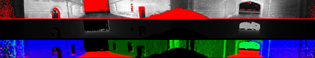
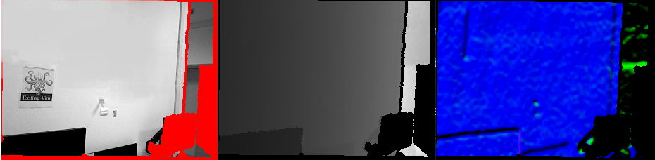
Figure 3: Cues generated for LiDAR (top) and RGB-D (bottom) images. The first row/column shows the intensity $\mathcal{I}^{i}$, the middle shows the range $\mathcal{I}^{\mathrm{\rho}}$, and the last one illustrates the normals encoded by color $\mathcal{I}^{\mathrm{n}}$. The red pixels on the intensity cues are invalid measurements (i.e., range not available).

IV-A Pyramid Generation

The first step to generate a pyramid from a pair of intensity $\mathcal{I}^{\mathrm{i}}$ and range image $\mathcal{I}^{\mathrm{\rho}}$ consists of extracting the normals. To calculate the normal at pixel $\mathbf{u}$ we unproject the pixels in the neighborhood $\mathcal{U}=\{\mathbf{u}^{\prime}:\|\mathbf{u}-\mathbf{u}^{\prime}\|<\tau_{\mathbf{u}}\}$ whose radius $\tau_{\mathbf{u}}$ is inversely proportional to the range at the pixel $I^{\rho}(\mathbf{u})$. The normal $\mathbf{n}_{\mathbf{u}}$ is the one of the plane that best fits the unprojected points from the set $\mathcal{U}$ . All valid normals are assembled in a normal image $\mathcal{I}^{\mathrm{n}}$, so that $\mathcal{I}^{\mathrm{n}}(\mathbf{u})=\mathbf{n}_{\mathbf{u}}$.

One level of a pyramid $\mathcal{I}$, therefore, consists of three images: $\mathcal{I}^{\mathrm{i}}$, $\mathcal{I}^{\mathrm{\rho}}$ and $\mathcal{I}^{\mathrm{n}}$. Further channels such as curvature and semantics can easily be embedded into the representation by adding additional images. In the remainder, we will refer to one general image in the set $\mathcal{I}$ as a cue $\mathcal{I}^{\mathrm{c}}$.

Pyramids are required to extend the basin of convergence of direct registration methods. This is due to the implicit data association, which operates only in the neighborhood of a few pixels. Hence, downscaling the images increases the convergence basin at the cost of reduced accuracy. However, the accuracy can be recovered by running the registration from the coarser to the finest level. Each time a level is changed, the initial guess of the transformation is set to the solution of the previous coarser level.

A pyramid $\mathcal{P}$ is generated from all the cues $\mathcal{I}=\{\mathcal{I}^{\mathrm{c}}\}$, by downscaling at user-selected resolutions. In our experiments, we typically use three scaling levels, each of them half the resolution of the previous level.

IV-B Direct Error Minimization

As in direct error minimization approaches, our method seeks to find the transform $\mathbf{X}^{*}\in\mathbb{SE}(3)$ that minimizes the photometric distance between the two images:

$$\small\mathbf{X}^{*}=\operatorname*{argmin}_{\mathbf{X}\in\mathbb{SE}(3)}\sum_{\mathbf{u}}\|\underbrace{\mathcal{\hat{I}}^{\mathrm{i}}(\mathbf{u})-\mathcal{I}^{\mathrm{i}}\overbrace{\left(\pi\left(\mathbf{X}\pi^{-1}\left(\mathbf{u},\rho\right)\right)\right)}^{\mathbf{u}^{\prime}}}_{\mathbf{e}_{\mathbf{u}}}\|^{2}$$ (10)

Where $\mathbf{e}^{\mathrm{i}}_{\mathbf{u}}$ denotes the error between corresponding pixels. The evaluation point $\mathbf{u}^{\prime}$ of $\mathcal{I}^{\mathrm{i}}$ is computed by unprojecting the pixel $\mathbf{u}$, applying the transform $\mathbf{X}$ and projecting it back. To carry out this operation, the range at the pixel $\rho=\mathcal{I}^{\rho}(\mathbf{u})$ needs to be known.

Eq. (10) models classical photometric error minimization assuming that the cues are not affected by the transform $\mathbf{X}$. In our case, range and normal are affected by $\mathbf{X}$. Hence, we need to account for the change in these cues, and we will do it by introducing a mapping function $\zeta^{\mathrm{c}}(\mathbf{X},\mathcal{\hat{I}}^{\mathrm{c}}(\mathbf{u}))$. This function calculates the pixel value of the $\mathrm{c}^{\mathrm{th}}$ cue after applying the transform $\mathbf{X}$ to the original channel value $\mathcal{\hat{I}}^{\mathrm{c}}(\mathbf{u})$. We can thus rewrite a more general form of Eq. (10) that accounts for all cues and captures this effect as follows:

$$\mathbf{X}^{*}=\operatorname*{argmin}_{\mathbf{X}\in\mathbb{SE}(3)}\sum_{\mathrm{c}}\sum_{\mathbf{u}}\|\underbrace{\zeta^{\mathrm{c}}(\mathbf{X},\mathcal{\hat{I}}^{\mathrm{c}}(\mathbf{u}))-\mathcal{I}^{\mathrm{c}}(\mathbf{u}^{\prime})}_{\mathbf{e}_{\mathbf{u}}^{c}}\|_{\mathbf{\Omega}^{\mathrm{c}}}^{2}$$ (11)

The squared Mahalanobis distance $\|\cdot\|^{2}_{\mathbf{\Omega}^{c}}$ is used to weight the different cues. More details about a general methodology for direct registration can be found in [4].

While approaching the problem in Eq. (11) with the ILS method described in Sec. III-A, particular care has to be taken to the numerical approximations of floating-point numbers. In particular, since each pixel and cue contribute to constructing the quadratic form with an independent error $\mathbf{e}_{\mathbf{u}}^{c}$, the summations in Eq. (4) might accumulate millions of terms. Hence, to lessen the effect of these round-offs, Eq. (4) has to be computed using a stable algorithm. In our single-threaded implementation, we use the compensated summation algoritm [11].

We use multi-cue direct alignment in incremental position tracking, explained in next section (Sec. IV-C) and in loop closure refinement and validation (Sec. IV-D).

IV-C Tracking

This module is in charge of estimating the open-loop trajectory of the sensor. To this extent, it processes new pyramids as they become available by determining the relative transform between the last pyramid $\mathcal{P}_{t}$, and the current keyframe $\mathcal{K}_{i}$. A keyframe stores a global transform $\mathbf{X}_{i}$, and a pyramid $\mathcal{P}_{i}$. The registration algorithm of Sec. IV-B is used to compute a relative transform $\mathbf{Z}_{i,t}$ between the last two pyramids. Whenever the magnitude of such a transform exceeds a given threshold or the overlap between $\mathcal{P}_{i}$ and $\mathcal{P}_{t}$ becomes too small, the tracker spawns a new keyframe $\mathcal{K}_{i+1}$, with transform $\mathbf{X}_{i+1}=\mathbf{X}_{i+1}\mathbf{Z}_{i,i+1}$. Furthermore, it adds to the graph a new constraint between the nodes $i$ and $i+1$, with transform $\mathbf{Z}_{i,i+1}$, and information matrix $\mathbf{\Omega}_{i,i+1}$. The latter is set to $\mathbf{H}$ matrix of the direct registration at the optimum. The generation of the new keyframe triggers the loop detection described in the next section. Using keyframes reduces the drift that would occur when performing subsequent pairwise registration since the reference frame stays fixed for a longer time. Potentially, if the sensor hovers at a distance smaller than the keyframe threshold, all registrations are done against the same pyramid, and no drift would occur.

IV-D Loop Detection and Validation

This module is responsible for relocalizing a newly generated keyframe with respect to previous ones. More formally, given a query frame $\mathcal{K}_{i}$, it retrieves a set of tuples $\{\left<\mathcal{K}_{j},\mathbf{Z}_{i,j},\mathbf{\Omega}_{i,j}\right>\}$, consisting of a past keyframe $\mathcal{K}_{j}$, a transform $\mathbf{Z}_{i,j}$ between $\mathcal{K}_{i}$ and $\mathcal{K}_{j}$ and an information matrix $\mathbf{\Omega}_{i,j}$ characterizing the uncertainty of the computed transform. Our system approaches loop closing in multiple stages. At first, we carry on visual place recognition on the intensity channels. This approach leverages the results of previous work [7]. For visual place recognition, we rely on ORB feature descriptors, extracted from the $\mathcal{I}^{\mathrm{i}}$ of each keyframe. Retrieving the most similar frame to the current one results in looking for the images in the database having the closest descriptor “close” to the one of the current image. To efficiently conduct this search, we use a hamming distance embedding binary search tree (HBST) [24], a tree-like structure that allows for descriptor search and insertion in logarithmic time by exploiting particular properties of binary descriptors. A match from HBST also returns a set of pairs of corresponding points between the matching keypoints. Having the depth and unprojecting the points, we can carry on a straightforward RANSAC registration. Finally, each candidate match is subject to direct refinement (Sec. IV-B). This step enhances the accuracy and it provides information matrices on the same scale as the ones generated by the tracker. The above strategy is applied independently to RGB-D or LiDAR data. These surviving pairs $\{\left<\mathcal{K}_{j},\mathbf{Z}_{i,j},\mathbf{\Omega}_{i,j}\right>\}$, constitute potential loop closing constraints to be added to the graph. However, to handle environments with large sensor aliasing, we introduced a further check to preserve topological consistency. Whenever a loop closure is found, we carry on a direct registration between all neighbours that would result after accepting the closure. If the resulting error is within certain bounds, the closure is finally added to the graph, and a global optimization is triggered.

IV-E Pose-graph Optimization

The goal of this module is to retrieve a configuration of the keyframes in the space that is maximally consistent with the incremental constraints introduced by the tracker and the loop closing constraints by the loop detector. A pose-graph is a special case of a factor graph [8, 15]. The nodes of the graph are the keyframe poses $\mathbf{X}=\{\mathbf{X}_{i}\}_{i=1:N}$, while the constraints encode the relative transformations between the connected keyframes, together with their uncertainty $\{\left<\mathbf{Z}_{i,j},\mathbf{\Omega}_{i,j}\right>\}$. Optimizing a factor graph consists in solving the following optimization problem:

$$\mathbf{X}^{*}=\operatorname*{argmin}_{\mathbf{X}\in\mathbb{SE}(3)^{N}}\sum_{i,j}\|\underbrace{\mathbf{X}_{i}^{-1}\mathbf{X}_{j}\boxminus\mathbf{Z}_{i,j}}_{\mathbf{e}_{i,j}}\|^{2}_{\mathbf{\Omega}_{i,j}}$$ (12)

Here, the error $\mathbf{e}_{i,j}$ is the difference between predicted displacement $\mathbf{X}_{i}^{-1}\mathbf{X}_{j}$ and result of the direct alignment $\mathbf{Z}_{i,j}$. The total perturbation vector $\mathbf{\Delta x}\in\mathbb{R}^{6N}$ results from stacking all variable perturbations $\{\mathbf{\Delta x}_{i}\}$.

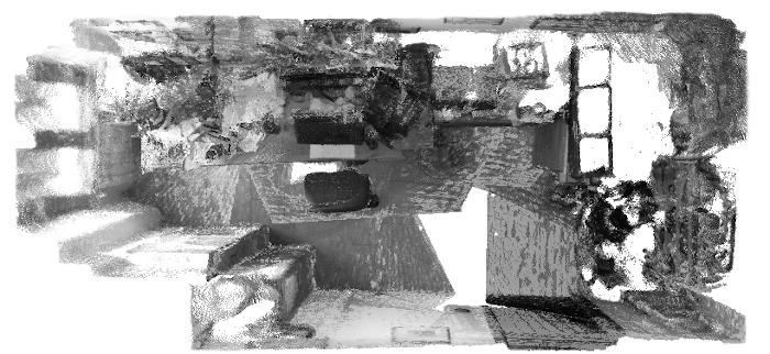
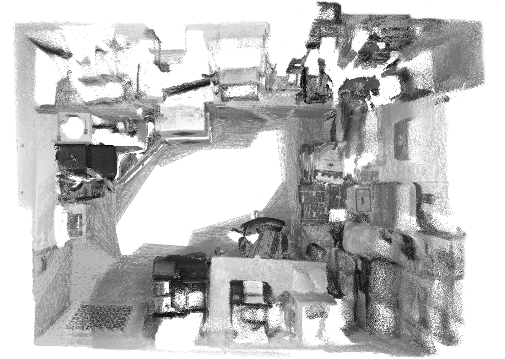
Figure 4: Qualitative RGB-D reconstructions showing the global consistency produced by our pipeline. Data has been self-recorded with an Intel Realsense 455.

V Experimental Evaluation

In this section, we report the results of our pipeline on different public benchmark datasets. To the best of our knowledge, our approach is the only open-source SLAM system that can deal with RGB-D and LiDAR in a unified manner. Therefore, to evaluate our system, we compare with state-of-the-art SLAM packages developed specifically for each of these sensor types. For RGB-D we consider DVO-SLAM [17] and ElasticFusion [31] as direct approaches and ORB-SLAM2 [19] as indirect representative. For LiDAR we compare against LeGO-LOAM [27] as feature-based and SuMA [2] representing the dense category.

To run the experiments, we used a PC with an Intel Core i7-7700K CPU @ 4.20GHz and 16GB of RAM. Since this work is focused on SLAM, we perform our quantitative evaluation using the RMSE on the absolute trajectory error (ATE) with $\mathbb{SE}(3)$ alignment. The alignment for the metric is computed by using the Horn method [12], and the timestamps are used to determine the associations. Then, we calculate the RMSE of the translational differences between all matched poses.

The tracking module dominates the runtime of our approach since loop closures are detected and validated asynchronously within another thread. Hence, we report the average frequency at which the tracker runs for each sensor. At the core of the tracker, we have the photometric registration algorithm, whose computation is proportional to the size of the images. Despite our current implementation of the registration algorithm being single-threaded, on the PC used to run the experiments, the tracking system runs at 5 Hz for the sensor with the highest resolution, while it can operate online on the sensor with the lowest resolution.

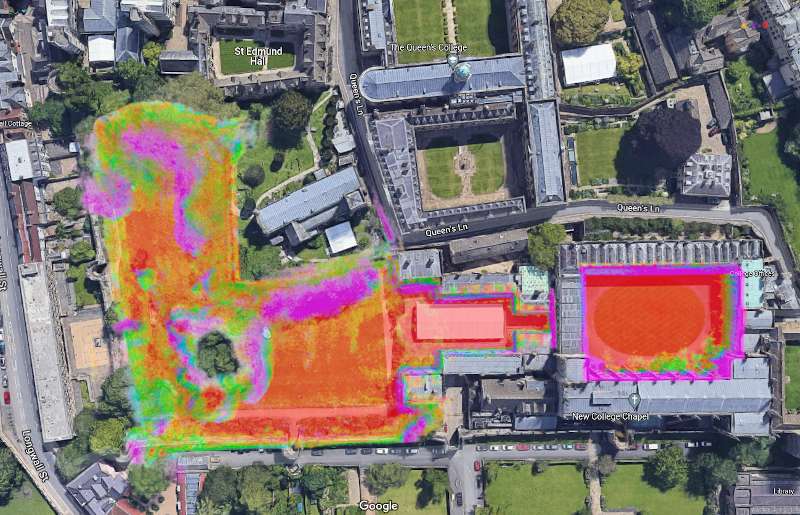
Figure 5: MD-SLAM map on long sequence from Newer College Dataset [21] aligned with Google Earth.

V-A RGB-D Results

We conducted several experiments with RGB-D sensor. Qualitative analysis have been done using self-recorded data and are shown in Fig. 4. As public benchmarks we used the TUM-RGB-D [29] and the ETH3D [25]. The TUM RGB-D dataset contains multiple real datasets captured with handheld Xbox Kinect. A rolling shutter camera provides RGB data. Further, the camera’s depth and color streams are not synchronized. Every sequence accompanies an accurate groundtruth trajectory obtained with an external motion capture system. ETH3D benchmark is acquired with global shutter cameras and accurate active stereo depth. Color and depth images are synchronized. We select several indoor sequences for which ground-truth, computed by external motion capture, is available.

On these datasets, we compare with DVO-SLAM, ElasticFusion and ORB-SLAM2. These three approaches are representative of different classes of SLAM algorithms. Tab. I shows the results on the TUM RGB-D datasets, while Tab. II presents the outcome on the ETH3D datasets. DVO SLAM implements a mixed geometry-based and direct registration. Internally the alignment between pairs of keyframes is obtained by jointly minimizing point-to-plane and photometric residuals. This is similar to ElasticFusion, whose estimate consists of a mesh model of the environment and the current sensor location instead of the trajectory. In contrast to these two approaches, ORB-SLAM2 implements a traditional visual SLAM pipeline, where a local map of landmarks around the RGB-D sensor is constructed from ORB features. This map is constantly optimized as the camera moves by performing local BA. Loop closures are detected through DBoW2 [6] and a global optimization on a $\mathbb{S}\mathrm{im}(3)$ pose-graph to enforce global consistency is used.

The TUM dataset provides images $640\times 480$ pixels, while ETH3D $740\times 460$ pixels. From these images, we compute a 3 level pyramid with scales $1/2$, $1/4$, and $1/8$. Our system runs respectively at $5.5$ and $5$ Hz at these resolutions.

	fr1/desk	fr1/desk2	fr2/desk
DVO-SLAM	$0.021$	$0.046$	$0.017$
ElasticFusion	$0.020$	$0.048$	$0.071$
ORB-SLAM2	0.016	0.022	0.009
Ours	$0.041$	$0.064$	$0.057$

TABLE I: ATE RMSE [m] results on TUM RGB-D datasets, recorded with non-synchronous depth using a rolling shutter camera.

	table3	table4	table7	cables1	plant2	planar2
DVO-SLAM	$0.008$	$0.018$	0.007	0.004	$0.002$	$0.002$
ElasticFusion	$-$	$0.012$	$-$	$0.018$	$0.017$	$0.011$
ORB-SLAM2	0.007	0.008	$0.010$	$0.007$	$0.003$	$0.005$
Ours	$0.021$	$0.022$	$0.036$	$0.015$	0.001	0.001

TABLE II: ATE RMSE [m] on ETH3D, recorded with global shutter camera and synchronous streams. ElasticFusion fails in table3 and table7.

In Tab. I we can see that ORB-SLAM2 clearly outperforms all other pipelines. DVO-SLAM and ElasticFusion provide comparable results, and our approach is the worst in terms of accuracy. Yet, the largest error is 6.4 cm, which results in a usable map. As stated before, this dataset is subject to rolling shutter and asynchronous depth effects. ORB-SLAM2, being feature-based, is less sensitive to these phenomena. DVO-SLAM and ElasticFusion explicitly model these effects. Our approach does not attempt to address these issues since it would render the whole pipeline less consistent between different sensing modalities.

Tab. II presents the results on the ETH3D benchmark. In this case, our performances are on par with other methods, since intensity and depth are synchronous, and the camera is global shutter.

These results highlight the strength and weaknesses of a purely direct approach not supported by any geometric association. While being compact, it suffers from unmodeled effects and requires a considerable overlap between subsequent frames.

V-B 3D LiDAR Results

We conducted different experiments on public LiDAR  benchmarks to show the performances of our SLAM implementation. For the LiDAR we use the Newer College Dataset [21, 35] recorded at 10 Hz with two models of Ouster LiDARs: OS1 and OS0. We conducted our evaluation on the long, cloister, quad-easy and stairs sequences. The OS1 has 64 vertical beams. We selected the long sequence that lasts approximately 45 minutes. It consists of multiple loops with viewpoint changes between buildings and a park.

The other three shorter sequences are recorded with the OS0, which has 128 vertical beams. The LiDAR  quad-easy sequence contains four loops that explore quad, cloister mixes outdoor and indoor scenes while stairs is purely indoor and based on vertical motion through different floors.

	OS0-128			OS1-64
	cloister	quad	stairs	long
LeGO-LOAM	0.20	0.09	$3.20$	1.30
SuMA	$3.34$	$1.74$	$0.67$	-
Ours	$0.36$	$0.25$	0.34	1.74

TABLE III: ATE RMSE [m] results of all benchmarked approaches on the Newer College Dataset. SuMA fails on long sequence.

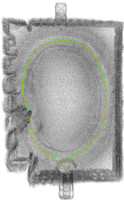
(a) quad-easy

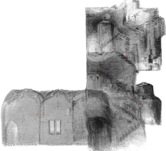
(b) stairs

Figure 6: Some scenes from Newer College dataset reconstructed by our system.

Qualitative analysis have been performed to show the results obtained by our pipeline. Fig. 6 illustrates some reconstructions obtained with MD-SLAM from Newer College sequences. Fig. 5 and Fig. 7 show the global consistency of our estimate on long sequence.

Quantitatively, we compare against LeGO-LOAM and SuMA. These represent two different classes of LiDAR algorithms, respectively sparse and dense. Tab. III summarizes the results of the comparison. LeGO-LOAM is currently one of the most accurate LiDAR SLAM pipelines and represents a sparse class of LiDAR algorithms. In contrast to our approach, LeGO-LOAM is a pure geometric feature-based frame-to-model LiDAR SLAM work, where the optimization on roll, yaw and z-axis (pointing up) is decoupled from the planar parameters. SuMa constructs a surfel-based map and estimates the changes in the sensor’s pose by exploiting the projective data association in a frame-to-model or in a frame-to-frame fashion. For both the pipelines loop closures are handled through ICP. Being ground optimized, LeGO-LOAM shows impressive results mainly in chunks where ground occupies most of the scene, yet our approach provides competitive accuracy. The situation becomes challenging for LeGO-LOAM when its assumptions are violated, such as in the stairs sequence. In this case, our pipeline is the most accurate since it does not impose any particular structure on the environment being mapped. SuMA performances are the worst in terms of accuracy. We tried this pipeline both in a frame-to-frame and frame-to-model mode. The one reported in Tab. III represents SuMA frame-to-frame that always outperforms the frame-to-model on these datasets.

We use the OS1 to produce images of $64\times 1024$ pixels while the OS0 to produce images of $128\times 1024$ pixels. Since the horizontal resolution is much larger than the vertical one, to balance the aspect ratio for direct registration, initially, we downscale the horizontal resolution by $1/2$ for OS0 and by $1/4$ for OS1. Our approach generates a pyramid with the following scales: $1$, $1/2$ and $1/4$. With these settings, our system operates at around 10 Hz on the OS0 and at approximately 20 Hz on the OS1, making it suitable for online estimation.

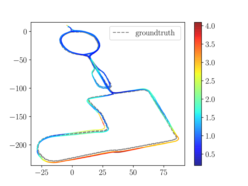
Figure 7: Alignment of our estimate with the groundtruth in long sequence of Newer College. The color bar on the right shows the translational error [m] over the whole trajectory.

VI Conclusion

In this paper, we presented a direct SLAM system that operates both with RGB-D and LiDAR sensors. These two heterogeneous sensor modalities are addressed exclusively by changing the projection models. To the best of our knowledge, our approach is the only open-source SLAM system that can deal with RGB-D and LiDAR in a unified manner. All optimization components in our system are dealt with a single ILS solver, resulting in highly compact code. Comparative experiments show that our generic method can compete with sensor-specific state-of-the-art approaches. Being purely photometric and without making any assumption of the environment, our pipeline shows consistent results on different types of datasets. We release our software as a C++ open-source package. The current single-thread implementation can operate online with small image sizes. Thanks to the inherent data-separation of direct registration, we envision a GPU implementation of our approach that seamlessly scales to high resolution while matching real-time requirements. Furthermore, the independence of the internal representation from the sensor source paves the way to SLAM systems that operate jointly on both RGB-D and LiDAR.

References

- [1] H. Bay, T. Tuytelaars, and L. Van Gool. Surf: Speeded up robust features. In Proc. of the Europ. Conf. on Computer Vision (ECCV), pages 404–417, 2006.
- [2] J. Behley and C. Stachniss. Efficient surfel-based slam using 3d laser range data in urban environments. In Proc. of Robotics: Science and Systems (RSS), 2018.
- [3] K. P. Cop, P. VK Borges, and R. Dubé. Delight: An efficient descriptor for global localisation using lidar intensities. In Proc. of the IEEE Intl. Conf. on Robotics & Automation (ICRA), pages 3653–3660, 2018.
- [4] B. Della Corte, I. Bogoslavskyi, C. Stachniss, and G. Grisetti. A general framework for flexible multi-cue photometric point cloud registration. In Proc. of the IEEE Intl. Conf. on Robotics & Automation (ICRA), pages 1–8, 2018.
- [5] J. Engel, T. Schöps, and D. Cremers. Lsd-slam: Large-scale direct monocular slam. In Proc. of the Europ. Conf. on Computer Vision (ECCV), pages 834–849, 2014.
- [6] D. Gálvez-López and J. D. Tardos. Bags of binary words for fast place recognition in image sequences. IEEE Trans. on Robotics (TRO), 28(5):1188–1197, 2012.
- [7] L. Di Giammarino, I. Aloise, C. Stachniss, and G. Grisetti. Visual place recognition using lidar intensity information. In Proc. of the IEEE/RSJ Intl. Conf. on Intelligent Robots and Systems (IROS), pages 4382–4389, 2021.
- [8] G. Grisetti, T. Guadagnino, I. Aloise, M. Colosi, B. Della Corte, and D. Schlegel. Least squares optimization: From theory to practice. Robotics, 9(3):51, 2020.
- [9] G. Grisetti, R. Kümmerle, H. Strasdat, and K. Konolige. g2o: A general framework for (hyper) graph optimization. In Proc. of the IEEE Intl. Conf. on Robotics & Automation (ICRA), pages 9–13, 2011.
- [10] J. Guo, P. VK Borges, C. Park, and A. Gawel. Local descriptor for robust place recognition using lidar intensity. IEEE Robotics and Automation Letters (RA-L), 4(2):1470–1477, 2019.
- [11] N. J. Higham. Accuracy and Stability of Numerical Algorithms. SIAM, 2002.
- [12] B. Horn, H. Hilden, and S. Negahdaripour. Closed-form solution of absolute orientation using orthonormal matrices. JOSA A, 5(7):1127–1135, 1988.
- [13] R. A. Newcombe S. Izadi, O. Hilliges, D. Molyneaux, D. Kim, A. J. Davison, P. Kohi, J. Shotton, S. Hodges, and A. Fitzgibbon. Kinectfusion: Real-time dense surface mapping and tracking. In Proc. of the Intl. Symposium on Mixed and Augmented Reality (ISMAR), pages 127–136, 2011.
- [14] E. Olson J. Serafin and G. Grisetti. Fast and robust 3d feature extraction from sparse point clouds. In Proc. of the IEEE/RSJ Intl. Conf. on Intelligent Robots and Systems (IROS), pages 4105–4112, 2016.
- [15] M. Kaess, A. Ranganathan, and F. Dellaert. isam: Incremental smoothing and mapping. IEEE Trans. on Robotics (TRO), 24(6):1365–1378, 2008.
- [16] M. Keller, D. Lefloch, M. Lambers, and S. Izadi. Realtime 3d reconstruction in dynamic scenes using pointbased fusion. In Proc. of the International Conference on 3D Vision (3DV), pages 1–8, 2013.
- [17] C. Kerl, J. Sturm, and D. Cremers. Dense visual slam for rgb-d cameras. In Proc. of the IEEE/RSJ Intl. Conf. on Intelligent Robots and Systems (IROS), pages 2100–2106, 2013.
- [18] M. Magnusson, H. Andreasson, A. Nüchter, and A. J. Lilienthal. Automatic appearance-based loop detection from three-dimensional laser data using the normal distributions transform. Journal of Field Robotics (JFR), 26(11-12):892–914, 2009.
- [19] R. Mur-Artal and J. D. Tardós. Orb-slam2: An open-source slam system for monocular, stereo, and rgb-d cameras. IEEE Trans. on Robotics (TRO), 33(5):1255–1262, 2017.
- [20] A. Nüchter, K. Lingemann, J. Hertzberg, and H. Surmann. Heuristic-based laser scan matching for outdoor 6d slam. In Annual Conf. on Artificial Intelligence, pages 304–319, 2005.
- [21] M. Ramezani, Y. Wang, M. Camurri, D. Wisth, M. Mattamala, and M. Fallon. The newer college dataset: Handheld lidar, inertial and vision with ground truth. In Proc. of the IEEE/RSJ Intl. Conf. on Intelligent Robots and Systems (IROS), pages 4353–4360, 2020.
- [22] T. Röhling, J. Mack, and D. Schulz. A fast histogram-based similarity measure for detecting loop closures in 3-d lidar data. In Proc. of the IEEE/RSJ Intl. Conf. on Intelligent Robots and Systems (IROS), pages 736–741, 2015.
- [23] E. Rublee, V. Rabaud, K. Konolige, and G. Bradski. Orb: An efficient alternative to sift or surf. In Proc. of the IEEE Intl. Conf. on Computer Vision (ICCV), pages 2564–2571, 2011.
- [24] D. Schlegel and G. Grisetti. Hbst: A hamming distance embedding binary search tree for feature-based visual place recognition. IEEE Robotics and Automation Letters (RA-L), 3(4):3741–3748, 2018.
- [25] T. Schops, T. Sattler, and M. Pollefeys. Bad slam: Bundle adjusted direct rgbd-d slam. In Proc. of the IEEE Conf. on Computer Vision and Pattern Recognition (CVPR), pages 134–144, 2019.
- [26] A. Segal, D. Haehnel, and S. Thrun. Generalized-icp. In Proc of Robotics: Science and Systems, 2009.
- [27] T. Shan and B. Englot. Lego-loam: Lightweight and ground-optimized lidar odometry and mapping on variable terrain. In Proc. of the IEEE/RSJ Intl. Conf. on Intelligent Robots and Systems (IROS), pages 4758–4765, 2018.
- [28] T. Stoyanov, M. Magnusson, H. Andreasson, and A. J. Lilienthal. Fast and accurate scan registration through minimization of the distance between compact 3d ndt representations. Intl. Journal of Robotics Research (IJRR), 31(12):1377–1393, 2012.
- [29] J. Sturm, N. Engelhard, F. Endres, W. Burgard, and D. Cremers. A benchmark for the evaluation of rgb-d slam systems. In Proc. of the IEEE/RSJ Intl. Conf. on Intelligent Robots and Systems (IROS), pages 573–580, 2012.
- [30] M. Velas, M. Spanel, and A. Herout. Collar line segments for fast odometry estimation from velodyne point clouds. In Proc. of the IEEE Intl. Conf. on Robotics & Automation (ICRA), pages 4486–4495, 2016.
- [31] T. Whelan, S. Leutenegger, R. Salas-Moreno, B. Glocker, and A. Davison. Elasticfusion: Dense slam without a pose graph. In Proc. of Robotics: Science and Systems, 2015.
- [32] B. Williams, G. Klein I., and Reid. Real-time slam relocalisation. In Proc. of the IEEE Intl. Conf. on Computer Vision (ICCV), pages 1–8, 2007.
- [33] J. Zhang and S. Singh. Loam: Lidar odometry and mapping in real-time. In Proc. of Robotics: Science and Systems (RSS), 2014.
- [34] J. Zhang and S. Singh. Visual-lidar odometry and mapping: Low-drift, robust, and fast. In Proc. of the IEEE Intl. Conf. on Robotics & Automation (ICRA), pages 2174–2181, 2015.
- [35] L. Zhang, M. Camurri, and M. Fallon. Multi-camera lidar inertial extension to the newer college dataset. arXiv, 2112.08854, 2021.