Differential Assessment of Black-Box AI Agents

Abstract

Much of the research on learning symbolic models of AI agents focuses on agents with stationary models. This assumption fails to hold in settings where the agent’s capabilities may change as a result of learning, adaptation, or other post-deployment modifications. Efficient assessment of agents in such settings is critical for learning the true capabilities of an AI system and for ensuring its safe usage. In this work, we propose a novel approach to differentially assess black-box AI agents that have drifted from their previously known models. As a starting point, we consider the fully observable and deterministic setting. We leverage sparse observations of the drifted agent’s current behavior and knowledge of its initial model to generate an active querying policy that selectively queries the agent and computes an updated model of its functionality. Empirical evaluation shows that our approach is much more efficient than re-learning the agent model from scratch. We also show that the cost of differential assessment using our method is proportional to the amount of drift in the agent’s functionality.

1 Introduction

With increasingly greater autonomy in AI systems in recent years, a major problem still persists and has largely been overlooked: how do we accurately predict the behavior of a black-box AI agent that is evolving and adapting to changes in the environment it is operating in? And how do we ensure its reliable and safe usage? Numerous factors could cause unpredictable changes in agent behaviors: sensors and actuators may fail due to physical damage, the agent may adapt to a dynamic environment, users may change deployment and use-case scenarios, etc. Most prior work on the topic presumes that the functionalities and the capabilities of AI agents are static, while some works start with a tabula-rasa and learn the entire model from scratch. However, in many real-world scenarios, the agent model is transient and only parts of its functionality change at a time.

Bryce, Benton, and Boldt (2016) address a related problem where the system learns the updated mental model of a user using particle filtering given prior knowledge about the user’s mental model. However, they assume that the entity being modeled can tell the learning system about flaws in the learned model if needed. This assumption does not hold in settings where the entity being modeled is a black-box AI system: most such systems are either implemented using inscrutable representations or otherwise lack the ability to automatically generate a model of their functionality (what they can do and when) in terms the user can understand. The problem of efficiently assessing, in human-interpretable terms, the functionality of such a non-stationary AI system has received little research attention.

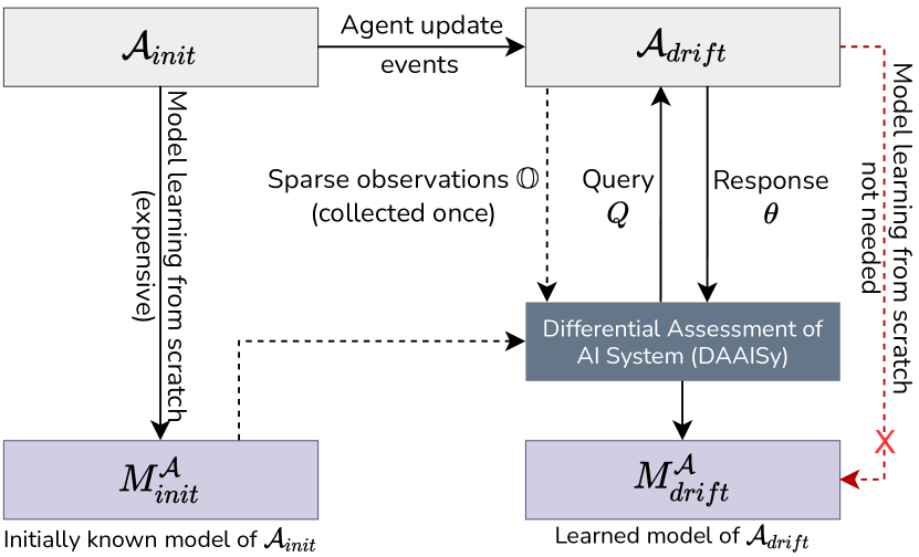
Figure 1: The Differential Assessment of AI System (DAAISy) takes as input the initially known model of the agent prior to model drift, available observations of the updated agent’s behavior, and performs a selective dialog with the black-box AI agent to output its updated model through efficient model learning.

The primary contribution of this paper is an algorithm for differential assessment of black-box AI systems (Fig. 1). This algorithm utilizes an initially known interpretable model of the agent as it was in the past, and a small set of observations of agent execution. It uses these observations to develop an incremental querying strategy that avoids the full cost of assessment from scratch and outputs a revised model of the agent’s new functionality. One of the challenges in learning agent models from observational data is that reductions in agent functionality often do not correspond to specific “evidence” in behavioral observations, as the agent may not visit states where certain useful actions are no longer applicable. Our analysis shows that if the agent can be placed in an “optimal” planning mode, differential assessment can indeed be used to query the agent and recover information about reduction in functionality. This “optimal” planning mode is not necessarily needed for learning about increase in functionality. Empirical evaluations on a range of problems clearly demonstrate that our method is much more efficient than re-learning the agent’s model from scratch. They also exhibit the desirable property that the computational cost of differential assessment is proportional to the amount of drift in the agent’s functionality.

Running Example

Consider a battery-powered rover with limited storage capacity that collects soil samples and takes pictures. Assume that its planning model is similar to IPC domain Rovers (Long and Fox 2003). It has an action that collects a rock sample at a waypoint and stores it in a storage iff it has at least half of the battery capacity remaining. Suppose there was an update to the rover’s system and as a result of this update, the rover can now collect the rock sample only when its battery is full, as opposed to at least half-charged battery that it needed before. Mission planners familiar with the earlier system and unaware about the exact updates in the functionality of the rover would struggle to collect sufficient samples. This could jeopardise multiple missions if it is not detected in time.

This example illustrates how our system could be of value by differentially detecting such a drift in the functionality of a black-box AI system and deriving its true functionality.

The rest of this paper is organized as follows: The next section presents background terminology. This is followed by a formalization of the differential model assessment problem in Section 3. Section 4 presents our approach for differential assessment by first identifying aspects of the agent’s functionality that may be affected (Section 4.1) followed by the process for selectively querying the agent using a primitive set of queries. We present empirical evaluation of the efficiency of our approach on randomly generated benchmark planning domains in Section 5. Finally, we discuss relevant related work in Section 6 and conclude in Section 7.

2 Preliminaries

We consider models that express an agent’s functionalities in the form of STRIPS-like planning models (Fikes and Nilsson 1971; McDermott et al. 1998; Fox and Long 2003) as defined below.

Definition 1.

A planning domain model is a tuple $M=\langle P,A\rangle$, where $P=\{p_{1}^{r_{1}},\dots,p_{n}^{r_{n}}\}$ is a finite set of predicates with arities $r_{i}$, $i\in[1,n]$; and $A=\{a_{1},\dots,a_{k}\}$ is a finite set of parameterized relational actions. Each action $a_{i}\in A$ is represented as a tuple $\langle header(a_{i}),\emph{pre}(a_{i}),\emph{eff}(a_{i})\rangle$, where $header(a_{i})$ represents the action header consisting of the name and parameters for the action $a_{i}$, $pre(a_{i})$ represents the conjunction of positive or negative literals that must be true in a state where the action $a_{i}$ is applicable, and $\emph{eff}(a_{i})$ is the conjunction of positive or negative literals that become true as a result of execution of the action $a_{i}$.

In the rest of the paper, we use the term “model” to refer to planning domain models and use closed-world assumption as used in the Planning Domain Definition Language (PDDL) (McDermott et al. 1998). Given a model $M$ and a set of objects $O$, let $S_{M,O}$ be the space of all states defined as maximally consistent sets of literals over the predicate vocabulary of $M$ with $O$ as the set of objects. We omit the subscript when it is clear from context. An action $a\in A$ is applicable in a state $s\in S$ if $s\models\emph{pre}(a)$. The result of executing $a$ is a state $a(s)=s^{\prime}\in S$ such that $s^{\prime}\models\emph{eff}(a)$, and all atoms not in $\emph{eff}(a)$ have literal forms as in $s$.

A literal corresponding to a predicate $p\in P$ can appear in $\emph{pre}(a)$ or $\emph{eff}(a)$ of an action $a\in A$ if and only if it can be instantiated using a subset of parameters of $a$. E.g., consider an action navigate (?rover ?src ?dest) and a predicate (can_traverse ?rover ?x ?y) in the Rovers domain discussed earlier. Suppose a literal corresponding to predicate (can_traverse ?rover ?x ?y) can appear in the precondition and/or the effect of navigate (?rover ?src ?dest) action. Assuming we know ?x and ?y in can_traverse, and ?src and ?dest in navigate are of the same type waypoint, the possible lifted instantiations of predicate can_traverse compatible with action navigate are (can_traverse ?rover ?src ?dest), (can_traverse ?rover ?dest ?src), (can_traverse ?rover ?src ?src), and (can_traverse ?rover ?dest ?dest). The number of parameters in a predicate $p\in P$ that is relevant to an action $a\in A$, i.e., instantiated using a subset of parameters of the action $a$, is bounded by the maximum arity of the action $a$. We formalize this notion of lifted instantiations of a predicate with an action as follows:

Definition 2.

Given a finite set of predicates $P=\{p_{1}^{r_{1}},\dots,p_{n}^{r_{n}}\}$ with arities $r_{i}$, $i\in[1,n]$; and a finite set of parameterized relational actions $A=\{a_{1}^{\psi_{1}},\dots,a_{k}^{\psi_{k}}\}$ with arities $\psi_{j}$ and parameters $\emph{par}(a_{j}^{\psi_{j}})=\langle\alpha_{1},\dots,\alpha_{\psi_{j}}\rangle$, $j\in[1,k]$, the set of lifted instantiations of predicates $P^{*}$ is defined as the collection $\{p_{i}(\sigma(x_{1}),\dots,\sigma(x_{r_{i}}))\,|p_{i}\in P,a\in A,\sigma:\{x_{1},\dots,x_{r_{i}}\}\rightarrow\emph{par}(a)\}$.

2.1 Representing Models

We represent a model $M$ using the set of all possible pal-tuples $\Gamma_{M}$ of the form $\gamma=\langle p,a,\ell\rangle$, where $a$ is a parameterized action header for an action in $A$, $p\in P^{*}$ is a possible lifted instantiation of a predicate in $P$, and $\ell\in$ {pre, eff} denotes a location in $a$, precondition or effect, where $p$ can appear. A model $M$ is thus a function $\mu_{M}:\Gamma_{M}\rightarrow\{+,-,\emptyset\}$ that maps each element in $\Gamma_{M}$ to a mode in the set $\{+,-,\emptyset\}$. The assigned mode for a pal-tuple $\gamma\in\Gamma_{M}$ denotes whether $p$ is present as a positive literal ($+$), as a negative literal ($-$), or absent ($\emptyset$) in the precondition ($\ell=$pre) or effect ($\ell=$ eff) of the action header $a$.

This formulation of models as pal-tuples allows us to view the modes for any predicate in an action’s precondition and effect independently. However, at times it is useful to consider a model at a granularity of relationship between a predicate and an action. We address this by representing a model $M$ as a set of pa-tuples $\Lambda_{M}$ of the form $\langle p,a\rangle$ where $a$ is a parameterized action header for an action in $A$, and $p\in P^{*}$ is a possible lifted instantiation of a predicate in $P$. Each pa-tuple can take a value of the form $\langle m_{\emph{pre}},m_{\emph{eff}}\rangle$, where $m_{\emph{pre}}$ and $m_{\emph{eff}}$ represents the mode in which $p$ appears in the precondition and effect of $a$, respectively. Since a predicate cannot appear as a positive (or negative) literal in both the precondition and effect of an action, $\langle+,+\rangle$ and $\langle-,-\rangle$ are not in the range of values that pa-tuples can take. Henceforth, in the context of a pal-tuple or a pa-tuple, we refer to $a$ as an action instead of an action header.

Measure of model difference

Given two models $M_{1}=\langle P,A_{1}\rangle$ and $M_{2}=\langle P,A_{2}\rangle$, defined over the same sets of predicates $P$ and action headers $A$, the difference between the two models $\Delta(M_{1},M_{2})$ is defined as the number of pal-tuples that differ in their modes in $M_{1}$ and $M_{2}$, i.e., $\Delta(M_{1},M_{2})=|\{\gamma\in P\times A\times\{+,-,\emptyset\}|\mu_{M_{1}}({\gamma})\neq\mu_{M_{2}}({\gamma})\}|$.

2.2 Abstracting Models

Several authors have explored the use of abstraction in planning (Sacerdoti 1974; Giunchiglia and Walsh 1992; Helmert, Haslum, and Hoffmann 2007; Bäckström and Jonsson 2013; Srivastava, Russell, and Pinto 2016). We define an abstract model as a model that does not have a mode assigned for at least one of the pal-tuples. Let $\Gamma_{M}$ be the set of all possible pal-tuples, and \raisebox{-.9pt} {?}⃝ be an additional possible value that a pal-tuple can take. Assigning \raisebox{-.9pt} {?}⃝ mode to a pal-tuple denotes that its mode is unknown. An abstract model $M$ is thus a function $\mu_{M}:\Gamma_{M}\rightarrow\{+,-,\emptyset,\raisebox{0.5pt}{\raisebox{-.9pt} {?}⃝}\}$ that maps each element in $\Gamma_{M}$ to a mode in the set $\{+,-,\emptyset,\raisebox{0.5pt}{\raisebox{-.9pt} {?}⃝}\}$. Let $\mathcal{U}$ be the set of all abstract and concrete models that can possibly be expressed by assigning modes in $\{+,-,\emptyset,\raisebox{0.5pt}{\raisebox{-.9pt} {?}⃝}\}$ to each pal-tuple $\gamma\in\Gamma_{M}$. We now formally define model abstraction as follows:

Definition 3.

Given models $M_{1}$ and $M_{2}$, $M_{2}$ is an abstraction of $M_{1}$ over the set of all possible pal-tuples $\Gamma$ iff $\exists\Gamma_{2}\subseteq\Gamma$ s.t. $\forall\gamma\in\Gamma_{2}$, $\mu_{M_{2}}(\gamma)=\raisebox{0.5pt}{\raisebox{-.9pt} {?}⃝}$ and $\forall\gamma\in\Gamma\setminus\Gamma_{2}$, $\mu_{M_{2}}(\gamma)=\mu_{M_{1}}(\gamma)$.

2.3 Agent Observation Traces

We assume limited access to a set of observation traces $\mathbb{O}$, collected from the agent, as defined below.

Definition 4.

An observation trace $o$ is a sequence of states and actions of the form $\langle s_{0},a_{1},s_{1},a_{2},\dots,s_{n-1},a_{n},s_{n}\rangle$ such that $\forall i\in[1,n]\;$ $a_{i}(s_{i-1})=s_{i}$.

These observation traces can be split into multiple action triplets as defined below.

Definition 5.

Given an observation trace $o=\langle s_{0},a_{1},s_{1},a_{2},\dots,s_{n-1},a_{n},s_{n}\rangle$, an action triplet is a 3-tuple sub-sequence of $o$ of the form $\langle s_{i-1},a_{i},s_{i}\rangle$, where $i\in[1,n]$ and applying an action $a_{i}$ in state $s_{i-1}$ results in state $s_{i}$, i.e., $a_{i}(s_{i-1})=s_{i}$. The states $s_{i-1}$ and $s_{i}$ are called pre- and post-states of action $a_{i}$, respectively.

An action triplet $\langle s_{i-1},a_{i},s_{i}\rangle$ is said to be optimal if there does not exist an action sequence (of length $\geq 1$) that takes the agent from state $s_{i-1}$ to $s_{i}$ with total action cost less than that of action $a_{i}$, where each action $a_{i}$ has unit cost.

2.4 Queries

We use queries to actively gain information about the functionality of an agent to learn its updated model. We assume that the agent can respond to a query using a simulator. The availability of such agents with simulators is a common assumption as most AI systems already use simulators for design, testing, and verification.

We use a notion of queries similar to Verma, Marpally, and Srivastava (2021), to perform a dialog with an autonomous agent. These queries use an agent to determine what happens if it executes a sequence of actions in a given initial state. E.g., in the rovers domain, the rover could be asked: what happens when the action sample_rock(rover1 storage1 waypoint1) is executed in an initial state $\{$(equipped_rock_analysis rover1), (battery_half rover1), (at rover1 waypoint1)$\}$?

Formally, a query is a function that maps an agent to a response, which we define as:

Definition 6.

Given a set of predicates $P$, a set of actions $A$, and a set of objects $O$, a query $Q\langle s,\pi\rangle:\mathcal{A}\rightarrow\mathbb{N}\times S$ is parameterized by a start state $s_{I}\in S$ and a plan $\pi=\langle a_{1},\dots,a_{N}\rangle$, where $S$ is the state space over $P$ and $O$, and $\{a_{1},\dots,a_{N}\}$ is a subset of action space over $A$ and $O$. It maps agents to responses $\theta=\langle n_{F},s_{F}\rangle$ such that $n_{F}$ is the length of the longest prefix of $\pi$ that $\mathcal{A}$ can successfully execute and $s_{F}\in S$ is the result of that execution.

Responses to such queries can be used to gain useful information about the model drift. E.g., consider an agent with an internal model $M_{\emph{drift}}^{\mathcal{A}}$ as shown in Tab. 1. If a query is posed asking what happens when the action sample_rock(rover1 storage1 waypoint1) is executed in an initial state $\{$(equipped_rock_analysis rover1), (battery_half rover1), (at rover1 waypoint1)$\}$, the agent would respond $\langle 0,\{$(equipped_rock_analysis rover1), (battery_half rover1), (at rover1 waypoint1)$\}\rangle$, representing that it was not able to execute the plan, and the resulting state was $\{$(equipped_rock_analysis rover1), (battery_half rover1), (at rover1 waypoint1)$\}$ (same as the initial state in this case). Note that this response is inconsistent with the model $M_{\emph{init}}^{\mathcal{A}}$, and it can help in identifying that the precondition of action sample_rock(?r ?s ?w) has changed.

3 Formal Framework

Our objective is to address the problem of differential assessment of black-box AI agents whose functionality may have changed from the last known model. Without loss of generality, we consider situations where the set of action headers is same because the problem of differential assessment with changing action headers can be reduced to that with uniform action headers. This is because if the set of actions has increased, new actions can be added with empty preconditions and effects to $M_{\emph{init}}^{\mathcal{A}}$, and if it has decreased, $M_{\emph{init}}^{\mathcal{A}}$ can be reduced similarly. We assume that the predicate vocabulary used in the two models is the same; extension to situations where the vocabulary changes can be used to model open-world scenarios. However, that extension is beyond the scope of this paper.

Model	Precondition		white[][0pt]Effect
$M^{\mathcal{A}}_{\emph{init}}$	(equipped_rock_analysis​ ?r)            (battery_half​ ?r)                         (at ?r ?w)	$\rightarrow$	white[][0pt](rock_sample_taken​ ?r)     (store_full ?r ?s)                     $\neg$(battery_half​ ​​?r)           (battery_reserve ?r)
$M^{\mathcal{A}}_{\emph{drift}}$	(equipped_rock_analysis​ ?r)                            (battery_full​ ?r)                          (at ?r ?w)	$\rightarrow$	white[][0pt](rock_sample_taken​ ?r)     (store_full ?r ?s)                     $\neg$(battery_full ?r)           (battery_half ?r)

Table 1: sample_rock (?r ?s ?w) action of the agent $\mathcal{A}$ in $M^{\mathcal{A}}_{\emph{init}}$ and a possible drifted model $M^{\mathcal{A}}_{\emph{drift}}$.

Suppose an agent $\mathcal{A}$’s functionality was known as a model $M_{\emph{init}}^{\mathcal{A}}=\langle P,\mathcal{A}_{\emph{init}}\rangle$, and we wish to assess its current functionality as the model $M_{\emph{drift}}^{\mathcal{A}}=\langle P,\mathcal{A}_{\emph{drift}}\rangle$. The drift in the functionality of the agent can be measured by changes in the preconditions and/or effects of all the actions in $\mathcal{A}_{\emph{init}}$. The extent of the drift between $M_{\emph{init}}^{\mathcal{A}}$ and $M_{\emph{drift}}^{\mathcal{A}}$ is represented as the model difference $\Delta(M_{\emph{init}}^{\mathcal{A}},M_{\emph{drift}}^{\mathcal{A}})$.

We formally define the problem of differential assessment of an AI agent below.

Definition 7.

Given an agent $\mathcal{A}$ with a functionality model $M_{\emph{init}}^{\mathcal{A}}$, and a set of observations $\mathbb{O}$ collected using its current version of $\mathcal{A}_{\emph{drift}}$ with unknown functionality $M_{\emph{drift}}^{\mathcal{A}}$, the differential model assessment problem $\langle M_{\emph{init}}^{\mathcal{A}},M_{\emph{drift}}^{\mathcal{A}},\mathbb{O},\mathcal{A}\rangle$ is defined as the problem of inferring $\mathcal{A}$ in form of $M_{\emph{drift}}^{\mathcal{A}}$ using the inputs $M_{\emph{init}}^{\mathcal{A}}$, $\mathbb{O}$, and $\mathcal{A}$.

We wish to develop solutions to the problem of differential assessment of AI agents that are more efficient than re-assessment from scratch.

3.1 Correctness of Assessed Model

We now discuss the properties that a model, which is a solution to the differential model assessment problem, should satisfy. A critical property of such models is that they should be consistent with the observation traces. We formally define consistency of a model w.r.t. an observation trace as follows:

Definition 8.

Let $o$ be an observation trace $\langle s_{0},a_{1},s_{1},a_{2},\dots,s_{n-1},a_{n},s_{n}\rangle$. A model $M=\langle P,A\rangle$ is consistent with the observation trace $o$ iff $\forall i\in\{1,..,n\}$ $\exists a\in A$ and $a_{i}$ is a grounding of action $a$ $\;s.t.\quad s_{i-1}\models\emph{pre}(a_{i})\;\land\;\forall\,l\in\emph{eff}(a_{i})\;s_{i}\models l$.

In addition to being consistent with observation traces, a model should also be consistent with the queries that are asked and the responses that are received while actively inferring the model of the agent’s new functionality. We formally define consistency of a model with respect to a query and a response as:

Definition 9.

Let $M=\langle P,A\rangle$ be a model; $O$ be a set of objects; $Q=\langle s_{I},\pi=\langle a_{1},\dots a_{n}\rangle\rangle$ be a query defined using $P,A,$ and $O$, and let $\theta=\langle n_{F},s_{F}\rangle$, ($n_{F}\leq n$) be a response to $Q$. $M$ is consistent with the query-response $\langle Q,\theta\rangle$ iff there exists an observation trace $\langle s_{I},a_{1},s_{1},\ldots,a_{n_{F}},s_{n_{F}}\rangle$ that $M$ is consistent with and $s_{n_{F}}\not\models\emph{pre}(a_{n_{F}+1})$ where $\emph{pre}(a_{n_{F}+1})$ is the precondition of $a_{n_{F}+1}$ in $M$.

We now discuss our methodology for solving the problem of differential assessment of AI systems.

4 Differential Assessment of AI Systems

Differential Assessment of AI Systems (Alg. 1) – DAAISy – takes as input an agent $\mathcal{A}$ whose functionality has drifted, the model $M_{\emph{init}}^{\mathcal{A}}=\langle P,A\rangle$ representing the previously known functionality of $\mathcal{A}$, a set of arbitrary observation traces $\mathbb{O}$, and a set of random states $\mathcal{S}\subseteq S$. Alg. 1 returns a set of updated models $\mathcal{M}^{\mathcal{A}}_{\emph{drift}}$, where each model $M_{\emph{drift}}^{\mathcal{A}}\in\mathcal{M}^{\mathcal{A}}_{\emph{drift}}$ represents $\mathcal{A}$’s updated functionality and is consistent with all observation traces $o\in\mathbb{O}$.

A major contribution of this work is to introduce an approach to make inferences about not just the expanded functionality of an agent but also its reduced functionality using a limited set of observation traces. Situations where the scope of applicability of an action reduces, i.e., the agent can no longer use an action $a$ to reach state $s^{\prime}$ from state $s$ while it could before (e.g., due to addition of a precondition literal), are particularly difficult to identify because observing its behavior does not readily reveal what it cannot do in a given state. Most observation based action-model learners, even when given access to an incomplete model to start with, fail to make inferences about reduced functionality. DAAISy uses two principles to identify such a functionality reduction. First, it uses active querying so that the agent can be made to reveal failure of reachability, and second, we show that if the agent can be placed in optimal planning mode, plan length differences can be used to infer a reduction in functionality.

DAAISy performs two major functions; it first identifies a salient set of pal-tuples whose modes were likely affected (line 1 of Alg. 1), and then infers the mode of such affected pal-tuples accurately through focused dialog with the agent (line 2 onwards of Alg. 1). In Sec. 4.1, we present our method for identifying a salient set of potentially affected pal-tuples that contribute towards expansion in the functionality of the agent through inference from available arbitrary observations. We then discuss the problem of identification of pal-tuples that contribute towards reduction in the functionality of the agent and argue that it cannot be performed using successful executions in observations of satisficing behavior. We show that pal-tuples corresponding to reduced functionality can be identified if observations of optimal behavior of the agent are available (Sec. 4.1). Finally, we present how we infer the nature of changes in all affected pal-tuples through a query-based interaction with the agent (Sec. 4.2) by building upon the Agent Interrogation Algorithm (AIA) (Verma, Marpally, and Srivastava 2021). Identifying affected pal-tuples helps reduce the computational cost of querying as opposed to the exhaustive querying strategy used by AIA. We now discuss the two major functions of Alg. 1 in detail.

Algorithm 1 Differential Assessment of AI Systems

Input:$M^{\mathcal{A}}_{\emph{init}}$, $\mathbb{O}$, $\mathcal{A}$, $\mathcal{S}$
Output: $\mathcal{M}^{\mathcal{A}}_{\emph{drift}}$

1:  $\Gamma_{\delta}\leftarrow\emph{identify\_affected\_pals()}$  

2:  $M_{\emph{abs}}\!\leftarrow\!$ set pal-tuples in $M_{\emph{init}}^{\mathcal{A}}$ corresponding to $\Gamma_{\delta}$ to \raisebox{-.9pt} {?}⃝ 

3:  $\mathcal{M}^{\mathcal{A}}_{\emph{drift}}$ $\leftarrow\{M_{\emph{abs}}\}$ 

4:  for each $\gamma$ in $\Gamma_{\delta}$ do

5:     for each $M_{\emph{abs}}$ in $\mathcal{M}^{\mathcal{A}}_{\emph{drift}}$ do

6:        $\mathcal{M}_{\emph{abs}}\leftarrow M_{\emph{abs}}\times\{\gamma^{+},\gamma^{-},\gamma^{\emptyset}\}$ 

7:        $\mathcal{M}_{\emph{sieved}}\leftarrow\{\}$

8:        if action corresponding to $\gamma$: $\gamma_{a}$ in $\mathbb{O}$ then

9:           $s_{\emph{pre}}\leftarrow\emph{states\_where\_}\gamma_{a}\emph{\_applicable}(\mathbb{O},\gamma_{a})$ 

10:           $Q\leftarrow\langle s_{\emph{pre}}\setminus\{\gamma_{p}\cup\neg\gamma_{p}$}, $\gamma_{a}$ $\rangle$ 

11:           $\theta\leftarrow\emph{ask\_query}(\mathcal{A},Q)$  

12:           $\mathcal{M}_{\emph{sieved}}\leftarrow\emph{sieve\_models}(\mathcal{M}_{\emph{abs}},Q,\theta)$ 

13:        else

14:           for each pair $\langle M_{i},M_{j}\rangle$ in $\mathcal{M}_{\emph{abs}}$ do

15:              $Q\leftarrow\emph{generate\_query}(M_{i},M_{j},\gamma,S)$ 

16:              $\theta\leftarrow\emph{ask\_query}(\mathcal{A},Q)$ 

17:              $\mathcal{M}_{\emph{sieved}}\leftarrow\emph{sieve\_models}(\{M_{i},M_{j}\},Q,\theta)$ 

18:           end for

19:        end if

20:        $\mathcal{M}_{\emph{abs}}\leftarrow\mathcal{M}_{\emph{abs}}\setminus$ $\mathcal{M}_{\emph{sieved}}$

21:     end for

22:     $\mathcal{M}^{\mathcal{A}}_{\emph{drift}}$ $\leftarrow\mathcal{M}_{\emph{abs}}$ 

23:  end for

4.1 Identifying Potentially Affected pal-tuples

We identify a reduced set of pal-tuples whose modes were potentially affected during the model drift, denoted by $\Gamma_{\delta}$, using a small set of available observation traces $\mathbb{O}$. We draw two kinds of inferences from these observation traces: inferences about expanded functionality, and inferences about reduced functionality. We discuss our method for inferring $\Gamma_{\delta}$ for both types of changes in the functionality below.

Expanded functionality

To infer expanded functionality of the agent, we use the previously known model of the agent’s functionality and identify its differences with the possible behaviors of the agent that are consistent with $\mathbb{O}$. To identify the pal-tuples that directly contribute to an expansion in the agent’s functionality, we perform an analysis similar to  Stern and Juba (2017), but instead of bounding the predicates that can appear in each action’s precondition and effect, we bound the range of possible values that each pa-tuple in $M_{\emph{drift}}^{\mathcal{A}}$ can take using Tab. 2. For any pa-tuple, a direct comparison between its value in $M_{\emph{init}}^{\mathcal{A}}$ and possible inferred values in $M_{\emph{drift}}^{\mathcal{A}}$ provides an indication of whether it was affected.

$\langle m_{\emph{pre}},m_{\emph{eff}}\rangle$	(pos,pos)	(pos,neg)	(neg,pos)	(neg,neg)
$\langle+,-\rangle$	✗	✓	✗	✗
$\langle+,\,\emptyset\,\rangle$	✓	✗	✗	✗
$\langle-,+\rangle$	✗	✗	✓	✗
$\langle-,\,\emptyset\,\rangle$	✗	✗	✗	✓
$\langle\,\emptyset\,,+\rangle$	✓	✗	✓	✗
$\langle\,\emptyset\,,-\rangle$	✗	✓	✗	✓
$\langle\,\emptyset\,,\,\emptyset\,\rangle$	✓	✗	✗	✓

Table 2: Each row represents a possible value $\langle m_{\emph{pre}},m_{\emph{eff}}\rangle$ for a pa-tuple $\langle p,a\rangle$. Each column represents a possible tuple representing presence of predicate $p$ in the pre- and post-states of an action triplet $\langle s_{i},a,s_{i+1}\rangle$ (discussed in Sec.4.1). The cells represent whether a value for pa-tuple is consistent with an action triplet in observation traces.

To identify possible values for a pa-tuple $\langle p,a\rangle$, we first collect a set of all the action-triplets from $\mathbb{O}$ that contain the action $a$. For a given predicate $p$ and state $s$, if $s\models p$ then the presence of predicate $p$ is represented as pos, similarly, if $s\models\neg p$ then the presence of predicate $p$ is represented as neg. Using this representation, a tuple of predicate presence $\in\{\emph{(pos,pos)}$, (pos,neg), (neg,pos), $\emph{(neg,neg)}\}$ is determined for the pa-tuple $\langle p,a\rangle$ for each action triplet $\langle s,a,s^{\prime}\rangle\in\mathbb{O}$ by analyzing the presence of predicate $p$ in the pre- and post-states of the action triplets. Possible values of the pa-tuple that are consistent with $\mathbb{O}$ are directly inferred from the Tab. 2 using the inferred tuples of predicate presence. E.g., for a pa-tuple, the values $\langle+,-\rangle$ and $\langle\emptyset,-\rangle$ are consistent with $(pos,neg)$, whereas, only $\langle\emptyset,+\rangle$ is consistent with $(pos,pos)$ and $(neg,pos)$ tuples of predicate presence that are inferred from $\mathbb{O}$.

Once all the possible values for each pa-tuple in $M_{\emph{drift}}^{\mathcal{A}}$ are inferred, we identify pa-tuples whose previously known value in $M_{\emph{init}}^{\mathcal{A}}$ is no longer possible due to inconsistency with $\mathbb{O}$. The pal-tuples corresponding to such pa-tuples are added to the set of potentially affected pal-tuples $\Gamma_{\delta}$. Our method also infers the correct modes of a subset of pal-tuples. E.g., consider a predicate $p$ and two actions triplets in $\mathbb{O}$ of the form $\langle s_{1},a,s_{1}^{\prime}\rangle$ and $\langle s_{2},a,s_{2}^{\prime}\rangle$ that satisfy $s_{1}\models p$ and $s_{2}\models\neg p$. Such an observation clearly indicates that $p$ is not in the precondition of action $a$, i.e., mode for $\langle p,a\rangle$ in the precondition is $\emptyset$. Such inferences of modes are used to update the known functionality of the agent. We remove such pal-tuples, whose modes are already inferred, from $\Gamma_{\delta}$.

A shortcoming of direct inference from successful executions in available observation traces is that it cannot learn any reduction in the functionality of the agent, as discussed in the beginning of Sec. 4. We now discuss our method to address this limitation and identify a larger set of potentially affected pal-tuples.

Reduced functionality

We conceptualize reduction in functionality as an increase in the optimal cost of going from one state to another. More precisely, reduction in functionality represents situations where there exist states $s_{i},s_{j}$ such that the minimum cost of going from $s_{i}$ to $s_{j}$ is higher in $M^{\mathcal{A}}_{\emph{drift}}$ than in $M_{\emph{init}}^{\mathcal{A}}$. In this paper, this cost refers to the number of steps between the pair of states as we consider unit action costs. This notion encompasses situations with reductions in reachability as a special case. In practice, a reduction in functionality may occur if the precondition of at least one action in $M^{\mathcal{A}}_{\emph{drift}}$ has new pal-tuples, or the effect of at least one of its actions has new pal-tuples that conflict with other actions required for reaching certain states.

Our notion of reduced functionality captures all the variants of reduction in functionality. However, for clarity, we illustrate an example that focuses on situations where precondition of an action has increased. Consider the case from Tab. 1 where $\mathcal{A}$’s model gets updated from $M_{\emph{init}}^{\mathcal{A}}$ to $M^{\mathcal{A}}_{\emph{drift}}$. The action sample_rock’s applicability in $M^{\mathcal{A}}_{\emph{drift}}$ has reduced from that in $M_{\emph{init}}^{\mathcal{A}}$ as $\mathcal{A}$ can no longer sample rocks in situations where the battery is half charged but needs a fully charged battery to be able to execute the action. In such scenarios, instead of relying on observation traces, our method identifies traces containing indications of actions that were affected either in their precondition or effect, discovers additional salient pal-tuples that were potentially affected, and adds them to the set of potentially affected pal-tuples $\Gamma_{\delta}$.

To find pal-tuples corresponding to reduced functionality of the agent, we place the agent in an optimal planning mode and assume limited availability of observation traces $\mathbb{O}$ in the form of optimal unit-cost state-action trajectories $\langle s_{0},a_{1},s_{1},a_{2},\dots,s_{n-1},a_{n},s_{n}\rangle$. We generate optimal plans using $M_{\emph{init}}^{\mathcal{A}}$ for all pairs of states in $\mathbb{O}$. We hypothesize that, if for a pair of states, the plan generated using $M_{\emph{init}}^{\mathcal{A}}$ is shorter than the plan observed in $\mathbb{O}$, then some functionality of the agent has reduced.

Our method performs comparative analysis of optimality of the observation traces against the optimal solutions generated using $M_{\emph{init}}^{\mathcal{A}}$ for same pairs of initial and final states. To begin with, we extract all the continuous state sub-sequences from $\mathbb{O}$ of the form $\langle s_{0},s_{1},\dots,s_{n}\rangle$ denoted by $\mathbb{O}_{\emph{drift}}$ as they are all optimal. We then generate a set of planning problems $\mathcal{P}$ using the initial and final states of trajectories in $\mathbb{O}_{\emph{drift}}$. Then, we provide the problems in $\mathcal{P}$ to $M_{\emph{init}}^{\mathcal{A}}$ to get a set of optimal trajectories $\mathbb{O}_{\emph{init}}$. We select all the pairs of optimal trajectories of the form $\langle o_{\emph{init}},o_{\emph{drift}}\rangle$ for further analysis such that the length of $o_{\emph{init}}\in\mathbb{O}_{\emph{init}}$ for a problem is shorter than the length of $o_{\emph{drift}}\in\mathbb{O}_{\emph{drift}}$ for the same problem. For all such pairs of optimal trajectories, a subset of actions in each $o_{\emph{init}}\in\mathbb{O}_{\emph{init}}$ were likely affected due to the model drift. We focus on identifying the first action in each $o_{\emph{init}}\in\mathbb{O}_{\emph{init}}$ that was definitely affected.

To identify the affected actions, we traverse each pair of optimal trajectories $\langle o_{\emph{init}},o_{\emph{drift}}\rangle$ simultaneously starting from the initial states. We add all the pal-tuples corresponding to the first differing action in $o_{\emph{init}}$ to $\Gamma_{\delta}$. We do this because there are only two possible explanations for why the action differs: (i) either the action in $o_{\emph{init}}$ was applicable in a state using $M_{\emph{init}}^{\mathcal{A}}$ but has become inapplicable in the same state in $M_{\emph{drift}}^{\mathcal{A}}$, or (ii) it can no longer achieve the same effects in $M_{\emph{drift}}^{\mathcal{A}}$ as $M_{\emph{init}}^{\mathcal{A}}$. We also discover the first actions that are applicable in the same states in both the trajectories but result in different states. The effect of such actions has certainly changed in $M_{\emph{drift}}^{\mathcal{A}}$. We add all the pal-tuples corresponding to such actions to $\Gamma_{\delta}$. In the next section, we describe our approach to infer the correct modes of pal-tuples in $\Gamma_{\delta}$.

4.2 Investigating Affected pal-tuples

This section explains how the correct modes of pal-tuples in $\Gamma_{\delta}$ are inferred (line 2 onwards of Alg.1). Alg. 1 creates an abstract model in which all the pal-tuples that are predicted to have been affected are set to \raisebox{-.9pt} {?}⃝ (line 2). It then iterates over all pal-tuples with mode \raisebox{-.9pt} {?}⃝ (line 4).

Removing inconsistent models

Our method generates candidate abstract models and then removes the abstract models that are not consistent with the agent (lines 7-18 of Alg. 1). For each pal-tuple $\gamma\in\Gamma$, the algorithm computes a set of possible abstract models $\mathcal{M}_{\emph{abs}}$ by assigning the three mode variants $+$, $-$, and $\emptyset$ to the current pal-tuple $\gamma$ in model $M_{\emph{abs}}$ (line 6). Only one model in $\mathcal{M}_{\emph{abs}}$ corresponds to the agent’s updated functionality.

If the action $\gamma_{a}$ in the pal-tuple $\gamma$ is present in the set of action triplets generated using $\mathbb{O}$, then the pre-state of that action $s_{\emph{pre}}$ is used to create a state $s_{I}$ (lines 9-10). $s_{I}$ is created by removing the literals corresponding to predicate $\gamma_{p}$ from $s_{\emph{pre}}$. We then create a query $Q\!=\!\langle s_{I},\langle\gamma_{a}\rangle\rangle$ (line 10), and pose it to the agent $\mathcal{A}$ (line 11). The three models are then sieved based on the comparison of their responses to the query $Q$ with that of $\mathcal{A}$’s response $\theta$ to $Q$ (line 12). We use the same mechanism as AIA for sieving the abstract models.

If the action corresponding to the current pal-tuple $\gamma$ being considered is not present in any of the observed action triplets, then for every pair of abstract models in $\mathcal{M}_{\emph{abs}}$ (line 14), we generate a query $Q$ using a planning problem (line 15). We then pose the query $Q$ to the agent (line 16) and receive its response $\theta$. We then sieve the abstract models by asking them the same query and discarding the models whose responses are not consistent with that of the agent (line 17). The planning problem that is used to generate the query and the method that checks for consistency of abstract models’ responses with that of the agent are used from AIA.

Finally, all the models that are not consistent with the agent’s updated functionality are removed from the possible set of models $\mathcal{M}_{\emph{abs}}$. The remaining models are returned by the algorithm. Empirically, we find that only one model is always returned by the algorithm.

4.3 Correctness

We now show that the learned drifted model representing the agent’s updated functionality is consistent as defined in Def. 8 and Def. 9. The proof of the theorem is available in the extended version of the paper (Nayyar, Verma, and Srivastava 2022).

Theorem 1.

Given a set of observation traces $\mathbb{O}$ generated by the drifted agent $\mathcal{A}_{\emph{drift}}$, a set of queries $Q$ posed to $\mathcal{A}_{\emph{drift}}$ by Alg. 1, and the model $M_{\emph{init}}^{\mathcal{A}}$ representing the agent’s functionality prior to the drift, each of the models $M=\langle P,A\rangle$ in $\mathcal{M}^{\mathcal{A}}_{\emph{drift}}$ learned by Alg. 1 are consistent with respect to all the observation traces $o\in\mathbb{O}$ and query-responses $\langle q,\theta\rangle$ for all the queries $q\in Q$.

There exists a finite set of observations that if collected will allow Alg. 1 to achieve 100% correctness with any amount of drift: this set corresponds to observations that allow line 1 of Alg. 1 to detect a change in the functionality. This includes an action triplet in an observation trace hinting at increased functionality, or a shorter plan using the previously known model hinting at reduced functionality. Thus, models learned by DAAISy are guaranteed to be completely correct irrespective of the amount of the drift if such a finite set of observations is available. While using queries significantly reduces the number of observations required, asymptotic guarantees subsume those of passive model learners while ensuring convergence to the true model.

5 Empirical Evaluation

In this section, we evaluate our approach for assessing a black-box agent to learn its model using information about its previous model and available observations. We implemented the algorithm for DAAISy in Python​​  and tested it on six planning benchmark domains from the International Planning Competition (IPC)​ . We used the IPC domains as the unknown drifted models and generated six initial domains at random for each domain in our experiments.

To assess the performance of our approach with increasing drift, we employed two methods for generating the initial domains: (a) dropping the pal-tuples already present, and (b) adding new pal-tuples. For each experiment, we used both types of domain generation. We generated different initial models by randomly changing modes of random pal-tuples in the IPC domains. Thus, in all our experiments an IPC domain plays the role of ground truth $M^{*}_{\emph{drift}}$ and a randomized model is used as $M_{\emph{init}}^{\mathcal{A}}$.

We use a very small set of observation traces $\mathbb{O}$ (single observation trace containing 10 action triplets) in all the experiments for each domain. To generate this set, we gave the agent a random problem instance from the IPC corresponding to the domain used by the agent. The agent then used Fast Downward (Helmert 2006) with LM-Cut heuristic (Helmert and Domshlak 2009) to produce an optimal solution for the given problem. The generated observation trace is provided to DAAISy as input in addition to a random $M_{\emph{init}}^{\mathcal{A}}$ as discussed in Alg. 1. The exact same observation trace is used in all experiments of the same domain, without the knowledge of the drifted model of the agent, and irrespective of the amount of drift.

We measure the final accuracy of the learned model $M_{\emph{drift}}^{\mathcal{A}}$ against the ground truth model $M^{*}_{\emph{drift}}$ using the measure of model difference $\Delta(M_{\emph{drift}}^{\mathcal{A}},M^{*}_{\emph{drift}})$. We also measure the number of queries required to learn a model with significantly high accuracy. We compare the efficiency of DAAISy (our approach) with the Agent Interrogation Algorithm (AIA) (Verma, Marpally, and Srivastava 2021) as it is the most closely related querying-based system.

All of our experiments were executed on 5.0 GHz Intel i9 CPUs with 64 GB RAM running Ubuntu 18.04. We now discuss our results in detail below.

5.1 Results

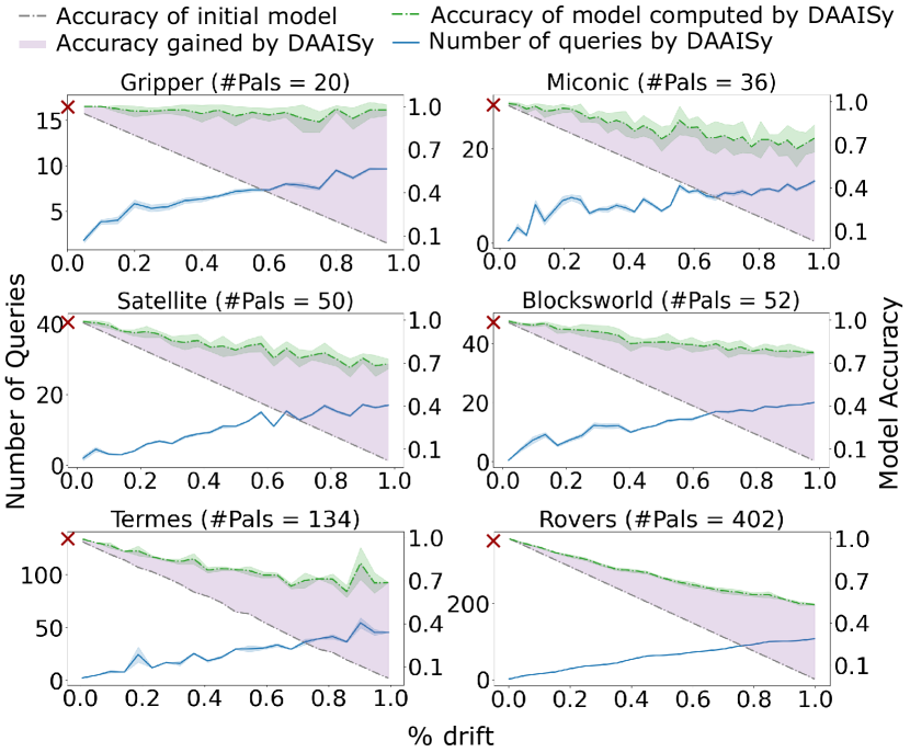
Figure 2: The number of queries used by DAAISy (our approach) and AIA (marked on y-axis), as well as accuracy of model computed by DAAISy with increasing amount of drift. Amount of drift equals the ratio of drifted pal-tuples and the total number of pal-tuples in the domains (nPals). The number of action triplets in the observation trace used for each domain is 10.

We evaluated the performance of DAAISy along 2 directions; the number of queries it takes to learn the updated model $M_{\emph{drift}}^{\mathcal{A}}$ with increasing amount of drift, and the correctness of the model $M_{\emph{drift}}^{\mathcal{A}}$ it learns compared to $M^{*}_{\emph{drift}}$.

Efficiency in number of queries

As seen in Fig. 2, the computational cost of assessing each agent, measured in terms of the number of queries used by DAAISy, increases as the amount of drift in the model $M^{*}_{\emph{drift}}$ increases. This is expected as the amount of drift is directly proportional to the number of pal-tuples affected in the domain. This increases the number of pal-tuples that DAAISy identifies as affected as well as the number of queries as a result. As demonstrated in the plots, the standard deviation for number of queries remains low even when we increase the amount of drift, showing the stability of DAAISy.

Comparison with AIA

Tab. 3 shows the average number of queries that AIA took to achieve the same level of accuracy as our approach for 50% drifted models, and DAAISy requires significantly fewer queries to reach the same levels of accuracy compared to AIA. Fig. 2 also demonstrates that DAAISy always takes fewer queries as compared to AIA to reach reasonably high levels of accuracy.

This is because AIA does not use information about the previously known model of the agent and thus ends up querying for all possible pal-tuples. DAAISy, on the other hand, predicts the set of pal-tuples that might have changed based on the observations collected from the agent and thus requires significantly fewer queries.

Correctness of learned model

DAAISy computes models with at least 50% accuracy in all six domains even when they have completely drifted from their initial model, i.e., $\Delta(M_{\emph{drift}}^{\mathcal{A}},M^{*}_{\emph{drift}})=$ nPals. It attains nearly accurate models for Gripper and Blocksworld for upto 40% drift. Even in scenarios where the agent’s model drift is more than 50%, DAAISy achieves at least 70% accuracy in five domains. Note that DAAISy is guaranteed to find the correct mode for an identified affected pal-tuple. The reason for less than $100\%$ accuracy when using DAAISy is that it does not predict a pal-tuple to be affected unless it encounters an observation trace conflicting with $M_{\emph{init}}^{\mathcal{A}}$. Thus, the learned model $M_{\emph{drift}}^{\mathcal{A}}$, even though consistent with all the observation traces, may end up being inaccurate when compared to $M^{*}_{\emph{drift}}$.

Domain	#Pals	AIA	DAAISy
Gripper	20	$15.0$	$6.5$
Miconic	36	$32.0$	$7.7$
Satellite	50	$34.0$	$9.0$
Blocksworld	52	$40.0$	$11.4$
Termes	134	$115.0$	$27.0$
Rovers	402	$316.0$	$61.0$

Table 3: The average number of queries taken by AIA to achieve the same level of accuracy as DAAISy (our approach) for 50% drifted models.

Discussion

AIA always ends up learning completely accurate models, but as noted above, this is because AIA queries exhaustively for all the pal-tuples in the model. There is a clear trade-off between the number of queries that DAAISy takes to learn the model as compared to AIA and the correctness of the learned model. As evident from the results, if the model has not drifted much, DAAISy can serve as a better approach to efficiently learn the updated functionality of the agent with less overhead as compared to AIA. Deciding the amount of drift after which it would make sense to switch to querying the model from scratch is a useful analysis not addressed in this paper.

6 Related Work

White-box model drift

Bryce, Benton, and Boldt (2016) address the problem of learning the updated mental model of a user using particle filtering given prior knowledge about the user’s mental model. However, they assume that the entity being modeled can tell the learning system about flaws in the learned model if needed. Eiter et al. (2005, 2010) propose a framework for updating action laws depicted in the form of graphs representing the state space. They assume that changes can only happen in effects, and that knowledge about the state space and what effects might change is available beforehand. Our work does not make such assumptions to learn the correct model of the agent’s functionalities.

Action model learning

The problem of learning agent models from observations of its behavior is an active area of research (Gil 1994; Yang, Wu, and Jiang 2007; Cresswell, McCluskey, and West 2009; Zhuo and Kambhampati 2013; Arora et al. 2018; Aineto, Celorrio, and Onaindia 2019). Recent work addresses active querying to learn the action model of an agent (Rodrigues et al. 2011; Verma, Marpally, and Srivastava 2021). However, these methods do not address the problem of reducing the computational cost of differential model assessment, which is crucial in non-stationary settings.

Online action model learning approaches learn the model of an agent while incorporating new observations of the agent behavior (Čertický 2014; Lamanna et al. 2021a, b). Unlike our approach, they do not handle cases where (i) the new observations are not consistent with the older ones due to changes in the agent’s behavior; and/or (ii) there is reduction in functionality of the agent. Lindsay (2021) solve the problem of learning all static predicates in a domain. They start with a correct partial model that captures the dynamic part of the model accurately and generate negative examples by assuming access to all possible positive examples. Our method is different in that it does not make such assumptions and leverages a small set of available observations to infer about increased and reduced functionality of an agent’s model.

Model reconciliation

Model reconciliation literature (Chakraborti et al. 2017; Sreedharan et al. 2019; Sreedharan, Chakraborti, and Kambhampati 2021) deals with inferring the differences between the user and the agent models and removing them using explanations. These methods consider white-box known models whereas our approach works with black-box models of the agent.

7 Conclusions and Future Work

We presented a novel method for differential assessment of black-box AI systems to learn models of true functionality of agents that have drifted from their previously known functionality. Our approach provides guarantees of correctness w.r.t. observations. Our evaluation demonstrates that our system, DAAISy, efficiently learns a highly accurate model of agent’s functionality issuing a significantly lower number of queries as opposed to relearning from scratch. In the future, we plan to extend the framework to more general classes, stochastic settings, and models. Analyzing and predicting switching points from selective querying in DAAISy to relearning from scratch without compromising the correctness of the learned models is also a promising direction for future work.

Appendix A Proofs of Theoretical Results

To prove Thm. 1 in the paper we will first need to prove that Tab. 2 is constructed correctly. We do this by using the following result:

Lemma 1.

Given an action triplet $\langle s,a,s^{\prime}\rangle\in\mathbb{O}$ and a predicate $p\in P$, Tab. 2 correctly represents the set of values for the pair of modes $\langle m_{\emph{pre}},m_{\emph{eff}}\rangle$, where $m_{\emph{pre}}$ and $m_{\emph{eff}}$ are the modes of predicate $p$ in the precondition and effect of action $a$ respectively, that are consistent with the action triplet.

Proof.

Given an action triplet $\langle s,a,s^{\prime}\rangle$, if a predicate $p\in P$ is true (or false) in $s$ (or $s^{\prime}$), then it cannot be false (or true) in the precondition (or effect) of $a$. Hence, if $p$ is true in both $s$ and $s^{\prime}$, its value for $\langle m_{\emph{pre}},m_{\emph{eff}}\rangle$ can only be $\langle+,\emptyset\rangle$, $\langle\emptyset,+\rangle$, or $\langle\emptyset,\emptyset\rangle$. If $p$ is true in $s$ but false in $s^{\prime}$, its value for $\langle m_{\emph{pre}},m_{\emph{eff}}\rangle$ can only be $\langle+,-\rangle$ or $\langle\emptyset,-\rangle$. If $p$ is false in $s$ but true in $s^{\prime}$, its value for $\langle m_{\emph{pre}},m_{\emph{eff}}\rangle$ can only be $\langle-,+\rangle$ or $\langle\emptyset,+\rangle$. Finally, if $p$ is false in both $s$ and $s^{\prime}$, its value for $\langle m_{\emph{pre}},m_{\emph{eff}}\rangle$ can only be $\langle-,\emptyset\rangle$, $\langle\emptyset,-\rangle$, or $\langle\emptyset,\emptyset\rangle$. Thus, for an observed action triplet $\langle s,a,s^{\prime}\rangle$, Tab. 2 shows all the possible values for a $p\in P$ in the precondition and effect of $a$ that do not conflict with the presence (or absence) of $p$ in $s$ and $s^{\prime}$ respectively. ∎

We now prove the two smaller results that combine to form Theorem 1.

Lemma 2.

Given a set of observation traces $\mathbb{O}$ generated by the drifted agent $\mathcal{A}_{\emph{drift}}$, each of the models $M=\langle P,A\rangle$ in $\mathcal{M}^{\mathcal{A}}_{\emph{drift}}$ learned by Alg. 1 are consistent with respect to all the observation traces $o\in\mathbb{O}$.

Proof.

Given that the action triplets in the set of observations $\mathbb{O}$ are generated using the same functionality of the deterministic agent after the drift $\mathcal{A}_{\emph{drift}}$ (i.e., all the observations correspond to the same drifted model), any two different action triplets in $\mathbb{O}$ containing groundings of the same action $a_{i}$ must have pre- and post-states that do not contradict each other. Now, for any action triplet $\langle s_{i-1},a_{i},s_{i}\rangle$ that is part of an observation trace $o\in\mathbb{O}$, when we consider the correct values for $\langle m_{\emph{pre}},m_{\emph{eff}}\rangle$ for a pa-tuple $\langle p,a_{i}\rangle$ such that $p\in P$, we only consider the values for $\langle m_{\emph{pre}},m_{\emph{eff}}\rangle$ that are shown in Tab. 2. For multiple actions triplets, possible values for $\langle m_{\emph{pre}},m_{\emph{eff}}\rangle$ can be found by taking an intersection of the sets of values for $\langle m_{\emph{pre}},m_{\emph{eff}}\rangle$ for each action triplet found using Tab. 2. Using Lemma 1, this ensures that the learned model $M$ is consistent with all the action triplets in an observation trace $o\in\mathbb{O}$. Since an observation trace is a sequence of action triplets, the learned model $M\in\mathcal{M}^{\mathcal{A}}_{\emph{drift}}$ is consistent with all the observation traces in the set of observation traces $\mathbb{O}$. ∎

Lemma 3.

Given a set of queries $Q$ posed to $\mathcal{A}_{\emph{drift}}$ by Alg. 1, and the model $M_{\emph{init}}^{\mathcal{A}}$ representing the agent’s functionality prior to the drift, each of the models $M=\langle P,A\rangle$ in $\mathcal{M}^{\mathcal{A}}_{\emph{drift}}$ learned by Alg. 1 are consistent with respect to all query-responses $\langle q,\theta\rangle$ for all the queries $q\in Q$.

Proof.

The agent responds to the query $q=\langle s_{I},\pi=\langle a_{1},\dots a_{n}\rangle\rangle$ using the drifted model with a response $\theta=\langle n_{F},s_{F}\rangle$. This response can only be generated if there exists an observation trace $\langle s_{I},a_{1},s_{1},\ldots,a_{n_{F}},s_{n_{F}}\rangle$ of length $n_{F}$ that can take the agent starting from state $s_{I}$ to the state $s_{n_{F}}$. Now, pruning models based on responses of the agent follows the criteria shown in Tab. 2. Hence, the only modes we consider for $p$ in the precondition and effect of $a_{n_{F}}$ are the ones that do not conflict with the presence (or absence) of $p$ in $s_{n_{F}-1}$ and $s_{n_{F}}$ respectively. The modes for any predicate in other actions are not fixed using responses to queries. Hence, the learned model $M\in\mathcal{M}^{\mathcal{A}}_{\emph{drift}}$ is consistent with all the query-responses $\langle q,\theta\rangle$ for all the queries $q\in Q$. ∎

Theorem 1.

Given a set of observation traces $\mathbb{O}$ generated by the drifted agent $\mathcal{A}_{\emph{drift}}$, a set of queries $Q$ posed to $\mathcal{A}_{\emph{drift}}$ by Alg. 1, and the model $M_{\emph{init}}^{\mathcal{A}}$ representing the agent’s functionality prior to the drift, each of the models $M=\langle P,A\rangle$ in $\mathcal{M}^{\mathcal{A}}_{\emph{drift}}$ learned by Alg. 1 are consistent with respect to all the observation traces $o\in\mathbb{O}$ and query-responses $\langle q,\theta\rangle$ for all the queries $q\in Q$.

Proof.

This theorem is conjunction of Lemma 1 and Lemma 2. Since both of the lemmas are proven to be true, this theorem is also true. ∎

References

- Aineto, Celorrio, and Onaindia (2019) Aineto, D.; Celorrio, S. J.; and Onaindia, E. 2019. Learning Action Models With Minimal Observability. Artificial Intelligence, 275: 104–137.
- Arora et al. (2018) Arora, A.; Fiorino, H.; Pellier, D.; Métivier, M.; and Pesty, S. 2018. A Review of Learning Planning Action Models. The Knowledge Engineering Review, 33: E20.
- Bäckström and Jonsson (2013) Bäckström, C.; and Jonsson, P. 2013. Bridging the Gap Between Refinement and Heuristics in Abstraction. In Proc. IJCAI.