Maximum entropy quantum state distributions

Abstract

We propose an approach to the realization of many-body quantum state distributions inspired by combined principles of thermodynamics and mesoscopic physics. Its essence is a maximum entropy principle conditioned by conservation laws. We go beyond traditional thermodynamics and condition on the full distribution of the conserved quantities. The result are quantum state distributions whose deviations from ‘thermal states’ get more pronounced in the limit of wide input distributions. We describe their properties in terms of entanglement measures and discuss strategies for state engineering by methods of current date experimentation.

In the early nineteenth century, thermodynamics was introduced to describe the state of complex systems on the basis of a minimal specification. The provided information would specify the values of certain macroscopic observables, such as the energy density. In the language of statistical thermodynamics, the minimal amount of information provided translates to maximal entropy of the remaining unspecified microscopic properties. For example, the canonical distribution $\rho=Z^{-1}\exp(-\beta H)$ defines a distribution for a system’s micro-states maximizing entropy under the condition of fixed average energy. The entropy, conditioned by the specified information, is $S=-\mathrm{tr}(\rho\ln\rho)$.

Two centennials later, the principles of that approach have not lost their power. However, progress in experimentation now makes it possible to apply them to quantum systems of mesoscopic proportions: systems large enough to be efficient information scramblers and ‘thermalizing’, yet small enough to harbor large quantum fluctuations. Under these conditions, it becomes natural to generalize the specified information from given average values of conserved quantities to full statistical distributions. For example, for a spin chain with conserved total $z$-axis magnetization, $S_{z}$, one may consider initial pure states $\hat{\rho}_{0}=|\Psi_{0}\rangle\langle\Psi_{0}|$ engineered to realize a chosen magnetization distribution $p(M)\equiv\langle\Psi_{0}|\delta_{\hat{S}_{z},M}|\Psi_{0}\rangle$. Under dynamical evolution by a Hamilton operator $\hat{H}(t)$ — assumed to be many-body chaotic — $\Psi_{0}$ evolves into a pseudo-random pure state, $\hat{\rho}=|\Psi\rangle\langle\Psi|$, with the same $p(M)$ (since $[\hat{H}(t),S_{z}]=0$), and perhaps other constraints, such as a conserved total energy. (By contrast, basic thermodynamics would be content with fixing just $\langle M\rangle=\langle\Psi|\hat{S}_{z}|\Psi\rangle$.)

In this letter we fuse concepts of thermodynamics and quantum mesosocopics. We consider pure states defined to maximize entropy, conditional that they realize a distribution $p(Q)$ of a scalar ‘charge’ , $Q$, — energy, particle number, uni-axial magnetization, etc. We describe the physical properties of such states, in particular their entanglement properties. The limiting case of $P(Q)=\delta_{Q,Q_{0}}$ models eigenstates of $\hat{Q}$ satisfying an eigenstate thermalization hypothesis (ETH) Deutsch (1991); Srednicki (1994); Rigol et al. (2008).

The key input determining the entanglement properties of our states are deviations between the specified distribution $p(Q)$ and the spectral distribution, $\Omega(Q)$, of the conserved operator, $\hat{Q}$, where $D\Omega(Q)$ is the number of $Q$-eigenvalue states in a $D$-dimensional Hilbert space. The unconstrained case, $p(Q)=\Omega(Q)$, has the highest entanglement, corresponding to Page’s maximally random pure states Page (1993). Constraining to eigenstates of $\hat{Q}$ reduces the entanglement, but much larger reductions can be obtained by specifying distributions broad compared to $\Omega(Q)$. Within a parameter space spanned by the center and width of $p(Q)$, we will discuss various reference configurations, among them Page’s random states Page (1993) (no input information provided), thermal distributions Sugiura and Shimizu (2012, 2013); Nakagawa et al. (2018), microcanonical distributions Vidmar and Rigol (2017); Bianchi et al. (2021), and very broadly distributed $p(Q)$. We will argue that for spin systems of mesoscopic proportions the engineering of the latter is in experimental reach and should thus lead to tunable non-thermal signatures in, e.g., Rényi entropies Islam et al. (2015); Kaufman et al. (2016) or spin-correlation probes.

Maximum entropy distributions:— Without much loss of generality, we consider a $N$-qubit system, and in it a conserved operator which is subsystem additive: a partition of the system into two subsystems $A$ and $B$ of size $N_{A}$ and $N_{B}=N-N_{A}$ implies a decomposition $\hat{Q}=\hat{Q}_{A}+\hat{Q}_{B}$. On the same basis, $\hat{Q}$’s eigenstates, $|n\rangle$ are labeled by a $D=2^{N}=2^{N_{A}+N_{B}}=D_{A}D_{B}$ dimensional index $n=(a,b)\in\mathbb{Z}_{2}^{N}$ with eigenvalues $Q_{n}$.

Assuming a given charge distribution, $p(Q)$, we now construct a distribution $P(\Psi)=P(\{\Psi_{n}\})$ defined on the space of pure states satisfying two conditions: first, in the limit of large $N$, states drawn from $P$ satisfy the condition $p(Q)=\langle\Psi|\delta_{\hat{Q},Q}|\Psi\rangle$, where $\delta_{\hat{Q},Q}$ is a $\delta$-function or a Kronecker $\delta$, depending on whether $Q$ is continuous or discrete. Second, the information entropy $S[P]=-\langle\ln(P)\rangle_{P}$ be maximal, where we introduced the shorthand notation $\langle\ldots\rangle_{P}=\int D\Psi P(\Psi)(\ldots)$. A distribution satisfying these criteria is found by extremizing the functional

$$A[P]\equiv S[P] +\lambda\left(\langle 1\rangle_{P}-1\right)+\lambda_{0}\left(\langle\langle\Psi|\Psi\rangle\rangle_{P}-1\right)$$

$$+\sum_{Q}\lambda(Q)\left(\langle\langle\Psi|\delta_{\hat{Q},Q}|\Psi\rangle\rangle_{P}-p(Q)\right).$$ (1)

Here, the Lagrange multipliers, $\lambda_{0}$ and $\lambda(Q)$ impose state normalization, $\langle\langle\Psi|\Psi\rangle\rangle_{P}=1$, and the distribution property, $\langle\langle\Psi|\delta_{\hat{Q},Q}|\Psi\rangle\rangle_{P}=p(Q)$, only on average over the distribution $P[\Psi]$. In exchange for the typicality assumption $\langle F[\Psi]\rangle_{\Psi}\approx F[\Psi]$, which we assume holds true in the limit of large Hilbert space dimension, we obtain an extremization problem that is easy to solve:

In the supplemental material sup , we show that the straightforward variation of the action functional yields the solution

$$\frac{D}{\lambda_{0}+\lambda(Q)}=\frac{p(Q)}{\Omega(Q)},\qquad\sum_{Q}\frac{D\Omega(Q)}{\lambda_{0}+\lambda(Q)}=1,$$ (2)

$$\rho_{n}\equiv\langle|\Psi_{n}|^{2}\rangle=\frac{p(Q_{n})}{D\Omega(Q_{n})}.$$ (3)

The first two of these equations fix the Lagrange multipliers, and the third states that the distribution of wave function amplitudes is Gaussian, with a variance set by the specified charge distribution $p(Q)$. With $\rho_{n}\geq 0$ and $\sum\rho_{n}=1$, we interpret $\rho=\{\rho_{n}\}$ as the average distribution of spectral weight over Fock space (see table 1 for an overview of the various distributions relevant to our discussion.)

To gain some familiarity with these expressions, consider the limiting case of unconstrained states, $\lambda(Q)=0$. The above equations are then solved by $\lambda_{0}=D$. For this value, $\Psi_{n}$ are Gaussian variables with uniform variance $D^{-1}$; the random state vectors considered by Page. In this particular case, the charge distribution $p(Q)=\Omega(Q)$ is dictated by the native spectral distribution. In the following, we consider what happens if we condition to Gaussian charge distributions

$$p(Q)=\frac{1}{\sqrt{2\pi}\Delta Q}\exp\left(-\frac{(Q-\bar{Q})^{2}}{2(\Delta Q)^{2}}\right),$$ (4)

of general center $\bar{Q}$ and width $\Delta Q$. The observation that the limiting case $p(Q)=\Omega(Q)$ corresponds to uniformly distributed states of minimal structure suggests to quantify the ‘input information’ provided by $p(Q)$ in terms of the statistical distance to $\Omega(Q)$, i.e. the Kullback-Leibler divergence $I_{\mathrm{in}}\equiv-D_{\mathrm{KL}}(p||\Omega)=\sum_{Q}p(Q)\ln\left(\frac{p(Q)}{\Omega(Q)}\right)$. Using Eqs.(2), it is straightforward to verify that

$$I_{\mathrm{in}}=-S(\rho)+\ln D,$$ (5)

where $S(\rho)=-\sum_{n}\rho_{n}\ln(\rho_{n})$ is the von Neumann entropy of the distribution $\rho$. In the following, we calculate the effects of this specified charge distribution $p(Q)$ on the entanglement entropies defined by subsystem partitions.

input	$\Omega(Q)$	spectral distribution of charge
	$p(Q)$	engineered distribution of charge
output	$P(\Psi)$	distribution of pure states conditioned via $p$
	$\rho_{n}$	spectral weight distribution in Fock space
	$\rho_{A,a}$	subsystem reduction of $\rho$
	$p_{A}(Q_{A})$	charge distribution over subsystem

Table 1: Overview over the different statistical distributions defined by a conserved operator $\hat{Q}$ in a many body system: the eigenvalues of $\hat{Q}$ are distributed according to $\Omega(Q)$; we are interested in states redistributing charge into $p(Q)$. Embedding this condition with the maximum entropy principle, we obtain average pure state distributions $\rho_{n}$, and their subsystem marginals $\rho_{A,a}$ for $n=(a,b)$. Finally, $p_{A}(Q_{A})$ describes the average distribution of charge on the subsystem $A$.

Entanglement entropies:— We cut our system into two pieces, $A$, $B$, with associated Fock spaces $\mathcal{F}=\mathcal{F}_{A}\otimes\mathcal{F}_{B}$ of dimensions $D_{A}\leq D_{B}$. For a given pure state $\hat{\rho}=|\Psi\rangle\langle\Psi|$, we consider the reduced density matrices $\hat{\rho}_{A}=\mathrm{tr}_{B}(\hat{\rho})$, and entanglement entropies $S=-\langle\mathrm{tr}(\hat{\rho}_{A}\ln\hat{\rho}_{A})\rangle_{\Psi}\simeq-\mathrm{tr}(\rho_{A}\ln\rho_{A})\equiv S^{\mathrm{a}}$, where in the ‘average’ entropy, $S^{\mathrm{a}}$, we assume self averaging $\hat{\rho}_{A}\simeq\langle\hat{\rho}_{A}\rangle_{\Psi}\equiv\rho_{A}$. Page has shown that in the absence of conditioning $S^{\mathrm{a}}=S_{\mathrm{th}}\equiv N_{A}\ln 2$ is trivially thermal. In the following we show how this changes due to specifying $p(Q)$. For a basis decomposition $n=(a,b)$, $\rho_{A}=\{\rho_{A,a}\}$ is described by a list of $D_{A}$ coefficients $\rho_{A,a}$. Using the definition of $S_{A}^{\mathrm{a}}$ in combination with Eq. (2), we obtain

$$\Delta S^{\mathrm{a}}=-\sum_{Q_{A}}p_{A}\ln\left(\frac{p_{A}}{\Omega_{A}}\right)=-D_{\mathrm{KL}}(p_{A}||\Omega_{A}),$$ (6)

$$\qquad p_{A}(Q_{A})=\Omega_{A}(Q_{A})\sum_{Q_{B}}\frac{\Omega_{B}(Q_{B})p(Q_{A}+Q_{B})}{\Omega(Q_{A}+Q_{B})},$$ (7)

for the difference $\Delta S^{\mathrm{a}}=S_{A}^{\rm av}-S_{\mathrm{th}}$. Conceptually, $p_{A}(Q_{A})$ describes the unit normalized foo (b) charge distribution imprinted on subsystem $A$ via the input charge distribution $p(Q)$ in the maximum entropy ensemble. Eq.  (6) states that the resulting reduction of the entanglement entropy of the average density matrix equals the (Kullback-Leibler) deviation of the induced distribution from the spectral distribution of the operator.

To make the result Eq. (6) concrete, we need to evaluate the convolutions in Eq. (6) in more explicit terms. Reflecting the local additivity principle obeyed by the variable $Q$, we assume that, except in the far tails of the spectrum, the density of states is Gaussian

$$\Omega(Q)=\Omega(Q,N)=\frac{1}{\sqrt{2\pi}\Gamma}e^{-\frac{Q^{2}}{2\Gamma^{2}}}\equiv\frac{1}{\sqrt{2\pi N}\gamma}e^{-N\frac{q^{2}}{2\gamma^{2}}},$$ (8)

where we define the $Q$-variable such that $Q=0$ corresponds to the center of the distribution $\Omega(Q)$, and the scaled variables $Q=Nq$, $\Gamma=\sqrt{N}\gamma$. The same function describes the subsystem spectral densities as $\Omega_{X}(Q_{X})=\Omega(Q_{X},N_{X})$, $X=A,B$.

In the supplemental material sup we show that for these spectral densities the reduced charge density assumes the form

$$p_{A}(Q_{A}) \approx\frac{N\sqrt{N_{B}}}{\Gamma\sqrt{2\pi N_{A}}}\int dx\,e^{-\frac{N_{A}N_{B}}{2\Gamma^{2}}x^{2}}p(q_{A}N+xN_{B}),$$ (9)

i.e. the input charge distribution convoluted against a smoothing function which knows about the spectral distribution of $\hat{Q}$ and the relative sizes of the subsystems. In the limit of large system sizes and fixed $N_{A}/N_{B}$, the variable $x\sim N^{-1/2}$, and so $xN_{B}\sim N^{1/2}$, which is small compared to the variable $q_{A}N\sim N$. For a broad input distribution, $p$, the $x$-dependence of $p$ becomes negligible, and the $x$-integral yields $p_{A}(Q_{A})\approx\frac{N}{N_{A}}p(Q_{A}(N/N_{A}))$. This result states that the charge distribution on $A$ inherits that of the system at large. In the opposite limit of a sharply-peaked input distribution, $p(Q)=\delta(Q-\bar{Q})$, Eq. (9) collapses to $p_{A}(Q_{A})\sim\exp(-\frac{N_{A}}{2\Gamma^{2}N_{B}}(q_{A}N-\bar{Q})^{2})$. This broadening of the $\delta$-function occurs due to the subsystem trace, which reduces the degree of constraint. More generally, for a Gaussian distribution of width $\Delta Q$ the computation of the entanglement entropy Eq. (6) (see supplemental material sup ) yields

$$\Delta S^{\mathrm{a}} =-\frac{n_{A}}{2}\left(\delta^{2}+\kappa^{2}-1\right)+\frac{1}{2}\ln\left(1+n_{A}\left(\delta^{2}-1\right)\right),$$

$$n_{A}=\frac{N_{A}}{N},\qquad\delta=\frac{\Delta Q}{\Gamma},\qquad\kappa=\frac{|\bar{Q}|}{\Gamma}.$$ (10)

According to this result, the state information output via the average entanglement entropy depends on the three parameters: relative system size, $n_{A}$; and deviation, $\kappa$, and width, $\delta$, of the input distribution relative to the width of $\hat{Q}$’s spectral density. Figure 1 shows this quantity for a centered distribution, $\kappa=0$, as a function of the parameter $\delta$ for multiple values of $n_{A}$. Its most striking feature is the non-monotonic dependence, with a minimum $\Delta S^{\mathrm{a}}=0$ for $\delta=1$, or $\Delta Q=\Gamma\propto N^{1/2}$ equal to the width of the native spectral distribution $\Omega(Q)$. The entanglement entropy may be reduced by sharpening the input distribution (thus increasing the specified information), with a limit $\Delta S^{\mathrm{a}}=(n_{A}+\ln{(1-n_{A})})/2$ for $\delta\rightarrow 0$. However, perhaps unexpectedly, output information also results from broadening the input. Already for distributions with $\delta\approx\sqrt{2}$, widening becomes a stronger information booster than sharpening. For extensively wide distributions, $\delta\sim\sqrt{N}$, or $\Delta Q\sim N$, the anomalous contribution to the entanglement entropy is likewise extensive, $\Delta S^{\mathrm{a}}\approx-n_{A}\delta^{2}\sim N_{A}$. (The extreme limit within this class of distributions is realized for a flat input $p(Q)=\mathrm{const}$. In this case, a straightforward estimate yields $\Delta S^{\mathrm{a}}\approx-N_{A}/24$, respecting the positive definiteness of the total entropy $S=S_{\mathrm{th}}+\Delta S^{\mathrm{a}}$.)

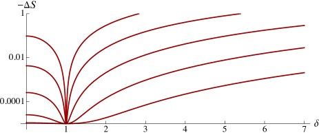
Figure 1: Entropy Eq. (6) plotted as a function of $\delta$ for $n_{A}=2^{-9},2^{-7},\ldots 2^{-1}$, with larger entropies corresponding to larger subsystem sizes.

Fluctuation corrections:— The above construction describes the entropy of the averaged state over a wide range of parameters. Quantitative corrections to Eq. (6) arise for average values $\bar{Q}$ in the far tails of the distribution $\Omega(Q)$, where the Gaussian distribution breaks down, or for input densities $p(Q)$ which cannot be modeled as locally Gaussian around a single maximum. While we do not consider such effects in the present paper, there remains one open conceptual point namely that the average entanglement entropy of pure states, $S\not=S^{\mathrm{av}}$ differs from that of the state-average. For example, Page has shown Page (1993) that in the absence of conditioning, $\Delta S^{\mathrm{a}}=0$, while for the full entanglement entropy, $\Delta S=-\frac{D_{A}}{2D_{B}}$ is exponentially small for asymmetric cuts, $D_{A}/D_{B}=2^{N_{A}-N_{B}}$, but becomes sizeable for near-equal subsystem sizes (see also  Foong and Kanno (1994); Sánchez-Ruiz (1995)).

In order to compute (quantum) fluctuation corrections to the result Eq. (6), we need to go back to a first principles representation $S=-\partial_{r}|_{r=1}M^{r}$ of the entanglement entropy in terms of the moments $M^{r}=\langle\mathrm{tr}_{A}(\hat{\rho}_{A}^{r})\rangle_{\Psi}$ of the reduced density matrix, $\rho_{A,aa^{\prime}}=\sum_{b}\Psi_{(ab)}\bar{\Psi}_{(a^{\prime}b)}$ Penington et al. (2019); Liu and Vardhan (2020). For the Gaussian distribution Eq. (11) this expression becomes a sum over all combinatorial pairings of wave function amplitudes, where so far we considered the nearest neighbor pairings, $\langle\Psi_{(ab)}\bar{\Psi}_{(a^{\prime}b)}\rangle_{\Psi}$. In the supplementary material sup we consider the contribution of other pairings for the exemplary case of the microcanonical distribution $p(Q)=\delta_{Q,\bar{Q}}$. (The computation for generic distributions is more complicated but does not lead to qualitatively different conclusions although details change.) It turns out that for $N_{A}\ll N_{B}$ and charges $\bar{Q}$ away from the extreme tails, the average entropy $S^{\mathrm{a}}$ approximates the full one up to corrections in $D_{A}/D_{B}$. (The scaling in Hilbert space dimensions follows from the observations that for Gaussian contractions different from the average one one needs to pay in free summations over the $B$-subspace.) For $N_{A}\approx N_{B}$, we obtain a correction, $\delta S$, required to establish the symmetry of the ‘entanglement wedge’ (see Fig. 2) under exchange $A\leftrightarrow B$. Technically, the wedge reflects zero singular values in the pure states Schmidt decomposition. For Page states these zeros only occur for $N_{B}>N_{A}$, however, it is more subtle in systems with conserved charges. In the supplemental material sup we show that for microcanonical distributions the ‘wedge’ is smoothened by a correction $\delta S\propto-\sqrt{N}\bar{q}$ (as first noted in Vidmar and Rigol (2017)). Higher order corrections in $D_{A}/D_{B}$ also considered by Page, on the other hand, remain bounded by $-1/2$ (see supplemental material sup for explicit expression). The upshot of this discussion is that for asymmetric cuts the average entropy approximates the full one, and even for equipartition $N_{A}=N_{B}$ represents a good approximation.

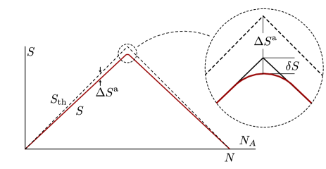
Figure 2: Schematic structure of the entanglement entropy as a function of subsystem size, $N_{A}$. Discussion, see text.

State preparation: — The above discussion has shown how maximum entropy states realizing broad charge distributions differ from thermal states. For systems in the thermodynamic limit $N\to\infty$, charge states lie with overwhelming probability inside the $\sim\sqrt{N}$ tolerance window of the native distribution $\propto D\Omega(Q)$, and the engineering of pure states of broader distribution may be hard. However, for the mesoscopic values of $N$ realized in current date AMO experiments or numerical analysis, broad distributions may be (perhaps even inadvertently) realized. To give an example, we consider a system of $N$ spin $1/2$ with assumed conservation of the total $z$-axis spin component, $\hat{Q}=\hat{S}_{z}$. Assume the system divided into $M=N/L$ blocks of $L$-sized cat states Johnson et al. (2017); Gao et al. (2010); Yao et al. (2012); Wang et al. (2016); Hacker et al. (2019); Duan (2019); Omran et al. (2019) $|\Psi_{a}\rangle=\frac{1}{\sqrt{2}}(|\uparrow\rangle_{L}+|\downarrow\rangle_{L})$ (with $|\uparrow,\downarrow\rangle_{L}$ the $\hat{Q}$-eigenstates at values $S_{z}=\pm L/2$), and consider $|\Psi\rangle\equiv\otimes_{a=1}^{M}|\Psi_{a}\rangle$. For this state, a straightforward calculation shows that $p(Q)=\langle\Psi|\delta_{Q,\hat{S}_{z}}|\Psi\rangle=\frac{1}{2^{M}}\sum_{a=0}^{M}\binom{M}{a}\delta_{Q,(a-\frac{M}{2})L}=\frac{1}{2^{M}}\binom{M}{\frac{M}{2}+\frac{Q}{L}}\simeq\frac{\sqrt{2}}{\sqrt{\pi M}}\exp(\frac{2Q^{2}}{ML^{2}})$. This particular state has charge distributed over a range $\sim L\sqrt{M}=N/\sqrt{M}$. This means that for fixed block number, $M\sim N^{0}$, we have an extensively broad distribution. In this scaling regime, the above product cat will evolve under chaotic time evolution into random states different from structureless ETH states. These differences show in the entanglement properties emphasized in this paper, but more directly also in magnetization probes revealing the dynamical conservation of the charge distribution despite the systems many body chaotic dynamics.

Discussion:— We introduced an approach to quantum state design which combines a maximum entropy principle with premeditated distributions of dynamically conserved observables in meso-sized many body quantum systems. This distribution survives unmasked by the chaotic dynamics and shows at various levels of the system description, beginning with the interpretation of the states themselves: for a given $p(Q)$, we defined a distribution of states $P(\Psi)$, such that individual states $\hat{\rho}=|\Psi\rangle\langle\Psi|$ drawn from it, generate the input in the sense $p(Q)=\mathrm{tr}(\hat{\rho}\delta_{\hat{Q},Q})$. (As an alternative to this pure state interpretation, one may also consider the mixed state $\hat{\rho}^{\prime}=\sum_{\Psi}P(\Psi)|\Psi\rangle\langle\Psi|$, which has the same property $p(Q)=\mathrm{tr}(\hat{\rho}\delta_{\hat{Q},Q})$, see supplemental material sup for more on the comparison of the two views.) When a component $B$ of the system is traced out and in this way becomes part of an environment, an induced charge distribution $\rho_{A}(Q_{A})$ emerges from the given one by a convolution over a kernel obtained from $\hat{Q}$’s spectral distribution, Eq. (9). This effective distribution is broader than the original one, reflecting the loss of information due to the partial trace. The statistical distance of the induced distribution to the spectral density of the conserved operator in $A$ determines the entanglement entropy of our quantum states, Eq.(6). This central result of our paper quantifies the difference to thermal states, a principal observation being that broad input distributions lead to the strongest deviations from ETH states. The straightforward generalization of this finding to multiple but mutually commuting conserved quantities (such as energy and particle number) shows that in this case the individually computed entropies $\Delta S^{\mathrm{a}}$ add. One point left out here concerns the generalization to distributions of strong non-Gaussianity. (For recent work discussing the influence of Lorentzian distributions on the statistics of quantum states we refer to Ref. Bogomolny and Sieber (2018); Monteiro et al. (2021))

Our analysis illustrates how entire distributions (and not just single average values) may survive ergodic chaotic time evolution. It would be interesting to see if this principle of state design may be turned into a creative resource. Conversely, one needs to watch out, especially in small or medium sized systems, and check if the application of the ETH hypothesis to a many body state might be incompatible with an (perhaps inadvertently) introduced defined initial charge distribution.

Acknowledgments: — D. A. H. thanks Shayan Majidy and Nicole Yunger Halpern for discussions. D. A. H. is supported in part by NSF QLCI grant OMA-2120757. T. M. acknowledge financial support by Brazilian agencies CNPq and FAPERJ. A. A. acknowledges partial support from the Deutsche Forschungsgemeinschaft (DFG) within the CRC network TR 183 (project grant 277101999) as part of projects A03.

I Supplementary Material

I.1 Solution of the variational equations for the state distribution

We here show how Eqs. (2) follow from variation of the functional Eq. (Maximum entropy quantum state distributions). The straightforward solution of the variational equation $\delta_{P}A[P]=0$ yields $P(\Psi)=\frac{1}{Z}e^{-\lambda_{0}\langle\Psi|\Psi\rangle-\sum_{Q}\lambda(Q)\langle\Psi|\delta_{\hat{Q},Q}|\Psi\rangle}$, with a normalization factor $Z$. Using the eigenstate property, $\langle\Psi|\delta_{\hat{Q},Q}|\Psi\rangle=\sum_{m}|\Psi_{m}|^{2}\delta_{Q_{m},Q}$, and integrating over all components $\Psi_{m\not=n}$ but one, we find that individual amplitudes $\Psi_{n}$ are Gaussian distributed with

$$\rho_{n}\equiv\langle|\Psi_{n}|^{2}\rangle=\frac{1}{\lambda_{0}+\lambda(Q_{n})}.$$ (11)

This result may now now be used to fix the Lagrange multipliers $\lambda_{0}$ and $\lambda(Q)$. Converting sums into integrals as $\sum_{n}F(Q_{n})=\sum_{Q}\Omega(Q)F(Q)$, the normalization condition yields $1=\langle\sum_{n}|\Psi_{n}|^{2}\rangle=\sum_{Q}\frac{D\Omega(Q)}{\lambda_{0}+\lambda(Q)}$. Treating the second condition in Eq. (Maximum entropy quantum state distributions) in the same manner, we obtain the first line in Eq. (2). Substitution of this result into Eq. (11) yields the second line.

I.2 The subsystem charge distribution, $p_{A}(Q_{A})$

In order to derive Eq. (9), we represent the subsystem charge distribution as an integral over Gaussian spectral densities,

$$p_{A}(Q_{A})=\frac{\mathcal{N}_{A}\mathcal{N}_{B}}{\mathcal{N}_{A\cup B}}N_{B}\int dq_{B}\,$$

$$\quad e^{-\frac{1}{2\gamma^{2}}\left(N_{A}q^{2}_{A}+N_{B}q^{2}_{B}-\frac{1}{N}(q_{A}N_{A}+q_{B}N_{B})^{2}\right)}p(q_{A}N_{A}+q_{B}N_{B}),$$

where we introduced scaled, and effectively continuous variables $Q_{X}=q_{X}N_{X}$, $X=A,B$. Considered as a function of $q_{A,B}$, the exponential function under the integral possesses the saddle points, $q_{B}=q_{A}$, indicating that the system favors charge equilibration over its subsystems. With $q_{B}=q_{A}+q$, the second order expansion of the integral around this saddle assumes the form Eq.(9).

An explicit representation, not relying on the above assumption, may be obtained for a Gaussian input distribution $p(Q)=\frac{\Delta Q}{\sqrt{2\pi}}\exp(-\frac{(Q-\bar{Q})^{2}}{2\Delta Q^{2}})$. In this case, the integral over $q$ yields

$$p_{A}(Q_{A}) =\frac{N}{N_{A}}\frac{1}{\sqrt{2\pi}\Lambda}\exp\left(-\frac{(Q_{A}\frac{N}{N_{A}}-\bar{Q})^{2}}{2\Lambda^{2}}\right),$$

$$\qquad\Lambda^{2}=\Gamma^{2}\frac{N_{B}}{N_{A}}+\Delta Q^{2}.$$

In the limit of a wide charge distribution $\Delta Q^{2}\gg\Gamma^{2}(N_{B}/N_{A})$, this effective Gaussian distribution reduces to $p_{A}(Q_{A})\approx\frac{N}{N_{A}}p(Q_{A}(N/N_{A}))$. More generally, however, we obtain a Gaussian distribution of enhanced width.

The computation of the KL-divergence Eq. (6) is now reduced to a straightforward Gaussian integral over the distributions $p_{A},\Omega_{A}$, and we obtain

$$S^{\mathrm{a}} =S_{\mathrm{th}}-\frac{N_{A}}{2N}\left(\frac{\Delta Q^{2}}{\Gamma^{2}}+\frac{\bar{Q}^{2}}{\Gamma^{2}}-1\right)+$$

$$\qquad+\frac{1}{2}\ln\left(1+\frac{N_{A}}{N}\left(\frac{\Delta Q^{2}}{\Gamma^{2}}-1\right)\right)$$

I.3 Derivation of the fluctuation entropy

We here compute the dominant fluctuation contributions to the entanglement entropy for the microcanonical charge distribution from the moments $M^{r}=\sum\langle\Psi_{a_{1}b_{1}}\bar{\Psi}_{a_{2}b_{1}}\Psi_{a_{2}b_{2}}\bar{\Psi}_{a_{3}b_{2}}\ldots\Psi_{a_{r}b_{r}}\bar{\Psi}_{a_{1}b_{r}}\rangle$. It will be instructive to first review the computation for the case considered by Page, where the Gaussian contraction over random state vectors yields a factor $\langle\Psi_{ab}\bar{\Psi}_{a^{\prime}b^{\prime}}\rangle=D^{-1}\delta_{a,a^{\prime}}\delta_{b,b^{\prime}}$. A contribution of maximal number, $r$, of $b$-index summations is obtained by Gaussian pairing $\langle\Psi_{a_{l}b_{l}}\bar{\Psi}_{a_{l+1}b_{l}}\rangle=D^{-1}\delta_{a_{l},a_{l+1}}$ for all $l$. This single pairing amounts to taking the average over the distribution prior to computing the moments, $\langle M^{r}\rangle\to\langle M\rangle^{r}$, as discussed in the first part of the paper. Stepping down in the index order, $N(r,2)=\binom{r}{2}$ terms with $r-1$ summations over $b$ and two over $a$ are obtained by one pairing outside the above order. The summation over indices for these two terms yields the estimate $M_{r}\approx D^{-r}\left(D_{B}^{r}D_{A}+\binom{r}{2}D_{B}^{r-1}D_{A}^{2}\right)$, and the straightforward differentiation with respect to $r$ gets us to the Page result, $S\approx N_{A}\ln 2+\frac{D_{A}}{2D_{B}}$ Page (1993). This observation conveys a number of messages: first, pairings of generic number of pairing permutations $1<l<(r-2)$ do not contribute. (Technically, they vanish in the replica limit $r\rightarrow 1$, up to corrections exponentially small in $D$.) Second, the single transposition fluctuation contribution, $l=1$, is exponentially small, except for $N_{A}\approx N_{B}$. Finally, the above results becomes wrong for $N_{A}>N_{B}$. The resolution to this problem lies in the inclusion of the opposite limit where just one $b$-summation results from the likewise unique pairing $\langle\bar{\Psi}_{a_{l}b_{l-1}}\Psi_{a_{l}b_{l}}\rangle=D^{-1}\delta_{b_{l-1},b_{l}}$. Finally, symmetry is restored by considering $\binom{r}{2}$ terms with one pairing outside this scheme, two summations over $b$, $r-1$ over $a$. The differentiation of these two terms gives $S\approx N_{B}\ln 2+\frac{D_{B}}{2D_{A}}$, i.e. Page with $A\leftrightarrow B$.

A closer inspection of the full sum, and of its convergence properties in the limit $r\rightarrow\infty$, shows that the terms with $(r,r-1)$ or $(2,1)$ summations over $b$ need to be kept, depending on whether $D_{B}$ is larger or smaller than $D_{A}$. In this way, one obtains the full ‘Page curve’, i.e. the entropy $S\approx N_{X}\ln 2+\frac{D_{X}}{2D_{\bar{X}}}$ with $(X,\bar{X})=(A,B)$ or $(B,A)$ depending on which of the systems is larger.

These general structures remain valid in the case of more general distributions, and specifically the microcanonical one with pairing $\langle\Psi_{ab}\bar{\Psi}_{a^{\prime}b^{\prime}}\rangle=\delta_{Q_{a}+Q_{b},\bar{Q}}(D\Omega(\bar{Q}))^{-1}\delta_{a,a^{\prime}}\delta_{b,b^{\prime}}$. Substituting these expressions into $M_{r}$, organizing the sum according to the number of $b$- and $a$-index summations, and trading the $a$ and $b$ summations for summations over $Q_{A}$ and $Q_{B}=\bar{Q}-Q_{A}$ weighted by spectral densities, we obtain the two alternative representations

$$M_{r} =\frac{1}{F(\bar{Q})^{r}}\sum_{Q_{A},Q_{B}}\delta_{Q_{A}+Q_{B},\bar{Q}}\sum_{k=1}^{r}N(r,k)\times$$ (12)

$$\qquad\times\left\{\begin{array}[]{l}F_{B}(Q_{B})^{r+1}\left(\frac{F_{A}(Q_{A})}{F_{B}(Q_{B})}\right)^{k}\cr F_{A}(Q_{A})^{r+1}\left(\frac{F_{B}(Q_{B})}{F_{A}(Q_{A})}\right)^{k}\end{array}\right.$$ (15)

with the abbreviations $F(\bar{Q})=D\Omega(\bar{Q})$, $F_{X}(Q_{X})=D_{X}\Omega_{X}(Q_{X})$, $X=A,B$, and combinatorial factors $N(r,1)=1$, $N(r,2)=\binom{r}{2},\ldots$ known as Narayana numbers. Convergence in the limit $r\to\infty$ (more precisely, the analytic properties of the representation of the sum over Narayana numbers in terms of hypergeometric functions Liu and Vardhan (2020); Penington et al. (2019)) implies that the first (second) of these defines an asymptotic $k$-series in the case $F_{A}(Q_{A})<F_{B}(Q_{B})$ ($F_{A}(Q_{A})>F_{B}(Q_{B})$). The terms $k=1,2$ are relevant to the computation of the entanglement entropy, and doing the $r$-derivative we obtain

$$S=-\sum_{Q_{A},Q_{B}}\delta_{Q_{A}+Q_{B},\bar{Q}}\left[\frac{F_{A}(Q_{A})F_{B}(Q_{B})}{F(\bar{Q})}\ln\left(\frac{F_{B}(Q_{B})}{F(\bar{Q})}\right)+\frac{1}{2}\frac{F^{2}_{A}(Q_{A})}{F(\bar{Q})}\right]\Theta(F_{B}(Q_{B})-F_{A}(Q_{A}))+(A\leftrightarrow B).$$ (16)

If $F_{A}(Q_{A})<F_{B}(Q_{B})$ for all terms in the sum, we are back to the result discussed in the main part of the paper, with corrections in $F_{A}/F\propto D_{A}/D_{B}$ from the second term. However, more sizeable modifications arise for larger subsystems, where swaps $F_{A}(Q_{A})>F_{B}(Q_{B})$ may occur for at least some terms under the sum.

For the Gaussian spectral densities, Eq. (8), the computation of these sums for general configurations $(\bar{Q},N_{A})$ is a straightforward if tedious affair. We here limit ourselves to the discussion of equal partitions, $N_{A}=N_{B}$, for which the strongest corrections to the previous results will be obtained. In this case, the case distinction in the above sum reduces to $\Theta(F_{B}(Q_{B})-F_{A}(Q_{A}))=\Theta(|Q_{A}|-|Q_{B}|)$, and assuming $\bar{Q}\geq 0$, this equals $\Theta(Q_{A}-\bar{Q}/2)$.

Comparing this expression to $S^{\mathrm{a}}$ studied in the main text — the first sum without $\Theta$-function constraint and $F^{2}_{A}/F$ correction — we find the deviation

$$\delta S\simeq\sum_{Q_{A}<\bar{Q}/2}\frac{F_{A}(Q_{A})F_{A}(\bar{Q}-Q_{A})}{F(\bar{Q})}\ln\left(\frac{F_{A}(Q_{A})}{F_{A}(\bar{Q}-Q_{A})}\right),$$

where we neglected the non-logarithmic as parametrically subleading (see below). Processing the $Q_{A}$-sum and the spectral density weights as in section I.2, we obtain (see also Ref. Vidmar and Rigol (2017))

$$\delta S\simeq-\frac{\sqrt{N}}{\sqrt{2\pi}\gamma}\int_{q_{A}<0}dq_{A}\,e^{-\frac{Nq^{2}_{A}}{2\gamma^{2}}}\left(\frac{N\bar{q}q_{A}}{\gamma^{2}}\right)=-\frac{\sqrt{N}\bar{q}}{\sqrt{2\pi}\gamma}.$$ (17)

A similar computation shows that the second term in angular brackets in Eq. (16) yields the correction

$$\delta S =-\frac{1}{2}e^{\frac{N\bar{q}^{2}}{2\gamma^{2}}}{\rm Erfc}\left(\frac{\sqrt{N}\bar{q}^{2}}{\sqrt{2\gamma^{2}}}\right),$$ (18)

with $\delta S\simeq-\gamma/(\sqrt{2\pi N}\bar{q})$ for $\bar{q}\gg\gamma/\sqrt{N}$ and cut off at $\delta S=-1/2$ for $\bar{q}=0$. We conclude that for generic values $\bar{q}\gtrsim\gamma/N^{-1/2}$, Eq. (17) defines the dominant fluctuation contribution to the entanglement entropy.

I.4 A note about distributions

There are at least three different distributions, defined over different support sets, that are relevant for our discussion. To define them, consider an operator $\hat{Q}$ with eigenstates $|n\rangle$ and eigenstates $Q_{n}\in I$ inside a certain interval.

1. The first (input distribution) is $p(Q)$ some distribution on $I$ one can choose at will.

2. The second is defined by a density matrix represented in the $\hat{Q}$ eigenbasis $\hat{\rho}=\sum_{n}\rho_{n}|n\rangle\langle n|$. The set of numbers $\{\rho_{n}\}$ defines a distribution on the set $\{n\}$ (i.e. according to Born’s rule, the probability to measure the outcome $Q_{n}$ in a measurement of $\hat{Q}$ is given by $\rho_{n}$).

3. The third is a distribution $P(\Psi)$ defined on the Hilbert space of states $\{\Psi\}$, i.e. a complex $D$-dimensional vector space.

To illustrate how these distributions are related to each other, we first note that distributions 2 and 3 individually define density matrices as

$$\hat{\rho}=\sum_{n}\rho_{n}|n\rangle\langle n|,\qquad\hat{\rho}^{\prime}=\int D\Psi\,P(\Psi)\,|\Psi\rangle\langle\Psi|,$$

where in the second expression $D\Psi=\prod_{n}d\Psi_{n}$. (Notice that we are here summing over a massively overcomplete set.) We can then establish a connection between the latter, requiring that the two representations $\hat{\rho}$ and $\hat{\rho}^{\prime}$ individually generate the input distribution 1. Conceptually, a distribution on the interval, $I$, is generated from one on $\{n\}$ by considering $Q_{n}$ as a random variable and $Q$ as a dependent random variable. (Much as e.g. the number parity is a dependent variable of $1,2,3,4,5,6$ when throwing a dice.) The distribution of $Q$ is then obtained from that of $Q_{n}$ as

$$p(Q)=\langle\delta_{Q,Q_{n}}\rangle_{\rho}\equiv\sum_{n}\rho_{n}\delta_{Q,Q_{n}}.$$ (19)

For example, if $\rho_{n}=Z^{-1}e^{-\lambda Q_{n}}$ is a canonical distribution, this becomes

$$p(Q)=\frac{1}{Z}\sum_{n}e^{-\lambda Q_{n}}\delta_{Q,Q_{n}}=\frac{D\Omega(Q)}{Z}e^{-\lambda Q},$$

with $Z=\sum_{n}e^{-\lambda Q_{n}}=D\sum_{Q}\Omega(Q)e^{-Q}$. In this way $\rho_{n}$ descends to a distribution $p(Q)$. In the same manner, the distribution $P(\Psi)$ generates a distribution $p(Q)$ too,

$$p(Q) =\langle\delta_{\hat{Q},Q}\rangle_{\Psi}\equiv\int D\Psi P(\Psi)\langle\Psi|\delta_{\hat{Q},Q}|\Psi\rangle.$$ (20)

Assuming Gaussianity $P(\Psi)=\mathcal{N}\prod_{n}e^{-c_{n}|\Psi_{n}|^{2}}$,

$$p(Q) =\sum_{n}c^{-1}_{n}\delta_{Q,Q_{n}}\equiv D\Omega(Q)c^{-1}(Q),$$ (21)

where in the final step we made the ansatz $c_{n}=c(Q_{n})$. If we now impose these induced density distributions to be equal, we get the identification

$$c(Q)=Ze^{\lambda Q}.$$ (22)

As a sanity check, we notice that the states described by the distribution $P(\Psi)$ are normalized (on average),

$$1 =\langle\langle\Psi|\Psi\rangle\rangle_{\Psi}$$

$$=\int D\Psi P(\Psi)\sum_{n}|\Psi_{n}|^{2}=\sum_{n}c_{n}^{-1}=Z^{-1}\sum_{n}e^{-\lambda Q_{n}}.$$

Summarizing, there is two a priori different density matrices $\hat{\rho}$ and $\hat{\rho}^{\prime}$ descending to the same ‘macroscopic’ charge distribution, and what remains to elaborate on their relation. To this end, we compare their matrix elements

$$\hat{\rho}_{nm}=\langle n|\hat{\rho}|m\rangle=\frac{1}{Z}\delta_{nm}e^{-\lambda Q_{n}},$$

and

$$\hat{\rho}^{\prime}_{nm} =\langle n|\hat{\rho}^{\prime}|m\rangle=\mathcal{N}\int D\Psi e^{-c_{n}|\Psi_{n}|^{2}}\Psi_{n}\bar{\Psi}_{m}=\frac{\delta_{nm}}{c_{n}}.$$ (23)

Employing that $c_{n}=c(Q_{n})$ given in Eq. (22), we conclude that

$$\hat{\rho}_{nm} =\hat{\rho}^{\prime}_{nm}.$$ (24)

That is, although defined in very different ways, both density matrices are actually equal.

References

- Deutsch (1991) J. M. Deutsch, Phys. Rev. A 43, 2046 (1991), URL https://link.aps.org/doi/10.1103/PhysRevA.43.2046.
- Srednicki (1994) M. Srednicki, Phys. Rev. E 50, 888 (1994), URL https://link.aps.org/doi/10.1103/PhysRevE.50.888.
- Rigol et al. (2008) M. Rigol, V. Dunjko, and M. Olshanii, Nature 452, 854 (2008), URL https://doi.org/10.1038/nature06838.
- Page (1993) D. N. Page, Phys. Rev. Lett. 71, 1291 (1993), URL https://link.aps.org/doi/10.1103/PhysRevLett.71.1291.
- Sugiura and Shimizu (2012) S. Sugiura and A. Shimizu, Phys. Rev. Lett. 108, 240401 (2012), URL https://link.aps.org/doi/10.1103/PhysRevLett.108.240401.
- Sugiura and Shimizu (2013) S. Sugiura and A. Shimizu, Phys. Rev. Lett. 111, 010401 (2013), URL https://link.aps.org/doi/10.1103/PhysRevLett.111.010401.
- Nakagawa et al. (2018) Y. O. Nakagawa, M. Watanabe, H. Fujita, and S. Sugiura, Nature Communications 9, 1635 (2018).
- Vidmar and Rigol (2017) L. Vidmar and M. Rigol, Phys. Rev. Lett. 119, 220603 (2017), URL https://link.aps.org/doi/10.1103/PhysRevLett.119.220603.
- Bianchi et al. (2021) E. Bianchi, L. Hackl, M. Kieburg, M. Rigol, and L. Vidmar, Volume-law entanglement entropy of typical pure quantum states (2021), eprint arXiv:2112.06959.
- Islam et al. (2015) R. Islam, R. Ma, P. M. Preiss, M. E. Tai, A. Lukin, M. Rispoli, and M. Greiner, Nature 528, 77 (2015), URL https://doi.org/10.1038/nature15750.
- Kaufman et al. (2016) A. M. Kaufman, M. E. Tai, A. Lukin, M. Rispoli, R. Schittko, P. M. Preiss, and M. Greiner, Science 353, 794 (2016), URL https://www.science.org/doi/abs/10.1126/science.aaf6725.
- (12) See supplementary material for (i) the solution of the variational equation, (ii) a discussion of the subsystem charge distribution , (iii) a derivation of the fluctuation entropy, and (iv) an alternative to the pure state interpretation.
- foo (b) The unit normalization follows from .
- Foong and Kanno (1994) S. K. Foong and S. Kanno, Phys. Rev. Lett. 72, 1148 (1994), URL https://link.aps.org/doi/10.1103/PhysRevLett.72.1148.
- Sánchez-Ruiz (1995) J. Sánchez-Ruiz, Phys. Rev. E 52, 5653 (1995), URL https://link.aps.org/doi/10.1103/PhysRevE.52.5653.
- Penington et al. (2019) G. Penington, S. H. Shenker, D. Stanford, and Z. Yang, Replica wormholes and the black hole interior (2019), eprint arXiv:1911.11977.
- Liu and Vardhan (2020) H. Liu and S. Vardhan, Entanglement entropies of equilibrated pure states in quantum many-body systems and gravity (2020), eprint arXiv:2008.01089.
- Johnson et al. (2017) K. G. Johnson, J. D. Wong-Campos, B. Neyenhuis, J. Mizrahi, and C. Monroe, Nature Communications 8, 697 (2017).
- Gao et al. (2010) W.-B. Gao, C.-Y. Lu, X.-C. Yao, P. Xu, O. Gühne, A. Goebel, Y.-A. Chen, C.-Z. Peng, Z.-B. Chen, and J.-W. Pan, Nature Physics 6, 331–335 (2010), ISSN 1745-2481, URL http://dx.doi.org/10.1038/nphys1603.
- Yao et al. (2012) X.-C. Yao, T.-X. Wang, P. Xu, H. Lu, G.-S. Pan, X.-H. Bao, C.-Z. Peng, C.-Y. Lu, Y.-A. Chen, and J.-W. Pan, Nature Photonics 6, 225–228 (2012), ISSN 1749-4893, URL http://dx.doi.org/10.1038/nphoton.2011.354.
- Wang et al. (2016) C. Wang, Y. Y. Gao, P. Reinhold, R. W. Heeres, N. Ofek, K. Chou, C. Axline, M. Reagor, J. Blumoff, K. M. Sliwa, et al., Science 352, 1087 (2016), URL https://www.science.org/doi/abs/10.1126/science.aaf2941.
- Hacker et al. (2019) B. Hacker, S. Welte, S. Daiss, A. Shaukat, S. Ritter, L. Li, and G. Rempe, Nature Photonics 13, 110–115 (2019), ISSN 1749-4893, URL http://dx.doi.org/10.1038/s41566-018-0339-5.
- Duan (2019) L. Duan, Nature Photon 13, 73–74 (2019), URL https://doi.org/10.1038/s41566-018-0340-z.
- Omran et al. (2019) A. Omran, H. Levine, A. Keesling, G. Semeghini, T. T. Wang, S. Ebadi, H. Bernien, A. S. Zibrov, H. Pichler, S. Choi, et al., Science 365, 570 (2019), URL https://www.science.org/doi/pdf/10.1126/science.aax9743.
- Bogomolny and Sieber (2018) E. Bogomolny and M. Sieber, Phys. Rev. E 98, 032139 (2018), URL https://link.aps.org/doi/10.1103/PhysRevE.98.032139.
- Monteiro et al. (2021) F. Monteiro, M. Tezuka, A. Altland, D. A. Huse, and T. Micklitz, Phys. Rev. Lett. 127, 030601 (2021), URL https://link.aps.org/doi/10.1103/PhysRevLett.127.030601.