Stability properties for a class of inverse problems

Abstract

We establish Lipschitz stability properties for a class of inverse problems. In that class, the associated direct problem is formulated by an integral operator ${\cal A}_{m}$ depending non-linearly on a parameter $m$ and operating on a function $u$. In the inversion step both $u$ and $m$ are unknown but we are only interested in recovering $m$. We discuss examples of such inverse problems for the elasticity equation with applications to seismology and for the inverse scattering problem in electromagnetic theory. Assuming a few injectivity and regularity properties for ${\cal A}_{m}$, we prove that the inverse problem with a a finite number of data points is solvable and that the solution is Lipschitz stable in the data. We show a reconstruction example illustrating the use of neural networks.

MSC 2010 Mathematics Subject Classification: 35R30, 47N20, 47N40.

Keywords: Stability properties of nonlinear inverse problems, integral operators, neural networks.

1 Introduction

Many physical phenomena are modeled by governing equations that depend linearly on some terms and non-linearly on other terms. For example, the wave equation may depend linearly on a forcing term and non-linearly on the medium velocity. Such inverse problems occur in passive radar imaging, or in seismology where the source of an earthquake has to be determined (the source could be a point, or a fault) and a forcing term supported on that source is also unknown. The inverse problem is then linear in the unknown forcing term and nonlinear in the location of the source.
In this paper, we establish Lipschitz stability properties for a related class of inverse problems which we introduce in section 2. In that class, the associated direct problem is formulated by an integral operator ${\cal A}_{m}$ depending non-linearly on a parameter $m$ and operating on a function $u$. In the inversion step, both $u$ and $m$ are unknown but we are only interested in recovering $m$. We discuss in section 3 examples of such inverse problems for the elasticity equation with applications to seismology and for the inverse scattering problem in electromagnetic theory. Assuming a few injectivity and regularity properties for ${\cal A}_{m}$, we prove in section 4 that the inverse problem solved from a finite number of data points $({\cal A}_{m}u(P_{j}))_{1\leq j\leq M}$ has a unique solution and that this solution is Lipschitz stable in the data (theorem 4.2).
Since this inverse problem is solvable we can define a function $\psi$ from the vector of data points in $\mathbb{R}^{M}$ to $m$. Under the general assumptions introduced in section 2, $\psi$ is Lipschitz continuous (with some insight on its Lipschitz norm discussed in section 4.3). Neural networks have been used as a tool for function approximation for some time. In our case the function $\psi$ is defined implicitly and in applications each evaluation of this function may be computationally expensive. It may thus be particularly convenient to pre-compute the vector $({\cal A}_{m}u(P_{j}))_{1\leq j\leq M}$ for many instances of $u$ and $m$ and use these pre-computed values in a learning algorithm that will determine the weights of a neural network ${\cal N}$ approximating $\psi$. It is however important to have some insight about how many layers and weights ${\cal N}$ should contain. Recently, asymptotic estimates on the size of neural networks have been derived [24, 15, 8]. These estimates involve the desired accuracy of the approximation, the dimension of the space where the function is defined, and importantly, the regularity of the function to be approximated. In particular, these estimates hold for Lipschitz regular functions and show that the accuracy increases in concert with the regularity of the function. However, high-order accuracy may be of little value in practical problems where only noisy inputs are available. In section 5 we show an example illustrating how a neural network ${\cal N}$ can approximate a function $\psi$, where $\psi$ solves a passive inverse elasticity problem. $\psi$ is known to be Lipschitz continuous thanks to the theory developed in section 4. This problem relates to a model in seismology. Applying ${\cal N}$ to a data vector $({\cal A}_{m}u(P_{j}))_{1\leq j\leq M}$ representing measurements of surface displacements yields $m$ which stands for the geometry parameter for a planar fault. While preparing data for the learning step and the learning itself are particularly long and costly (on the order of several hours on a high performance platform with multiple CPUs), applying ${\cal N}$ is fast (a few hundredths of a second for 500 evaluations). Our computational work shows that ${\cal N}$ performs well on noisy data too. If more information on uncertainty is needed in the case of noisy data, then the output from ${\cal N}$ can be used as a starting point for a sampling algorithm aimed at evaluating the covariance of $m$, or possibly its probability distribution function. The author proposed in [18] a parallel sampling algorithm that alternates computing proposals in parallel and combining proposals to accept or reject them.This algorithm, inspired by [4], is well-suited to inverse problems mixing linear and nonlinear terms, where some unknown amount of regularization is necessary, and where proposals are expensive to compute. The results from [18] compare favorably to those obtained from the Maximum Likelihood (ML), the Generalized Cross Validation (GCV), or the Constrained Least Squares (CLS) algorithms.

2 Statement of inverse problem

2.1 Notations and assumptions

Let $R$ and $V$ be two compact manifolds embedded in $\mathbb{R}^{d}$. Let ${\itbf H}_{m}:V\times R\rightarrow\mathbb{R}$ be an integration kernel depending on a parameter $m$, where $m$ is in a compact subset $B$ of $\mathbb{R}^{p}$. Let ${\cal A}_{m}$ be the operator defined by convolution by ${\itbf H}_{m}$

$${\cal A}_{m}g(x)=\int_{R}{\itbf H}_{m}(x,y)g(y)d\sigma(y),$$ (2.1)

where $d\sigma(y)$ is the surface measure on $R$. We assume that ${\itbf H}_{m}$ presents the following regularity properties:

1. $(m,x,y)\rightarrow{\itbf H}_{\itbf m}(x,y)$ is continuous in $B\times V\times R$ and the gradient in $x$, $(m,x,y)\rightarrow\nabla_{x}{\itbf H}_{m}(x,y)$, exists and is continuous in $B\times V\times R$.

2. There is an open set $B^{\prime}$ of $\mathbb{R}^{p}$ such that $B\subset B^{\prime}$ and the derivatives $(m,x,y)\rightarrow\partial_{m_{i}}{\itbf H}_{m}(x,y)$ and $(m,x,y)\rightarrow\partial_{m_{i}}\nabla_{x}{\itbf H}_{m}(x,y)$, exist and are continuous in $B^{\prime}\times V\times R$, where $1\leq i,j\leq p$.

Given (2.1) and assumption ($R_{2}$), we can define the directional derivative $\partial_{{\itbf q}}{\cal A}_{m}=\nabla_{m}{\cal A}_{m}\cdot{\itbf q}$ of the operator ${\cal A}_{m}$ for any unit vector ${\itbf q}$ of $\mathbb{R}^{p}$ and $m$ in $B^{\prime}$.

We make the following uniqueness assumptions:

1. For any $m,m^{\prime}$ in $B$ and any $u,v$ in $H^{1}_{0}(R)$, if ${\cal A}_{m}u={\cal A}_{m^{\prime}}v$ in $L^{2}(V)$ and $u\neq 0$ or $v\neq 0$, then $m=m^{\prime}$ and $u=v$. In particular, ${\cal A}_{m}$ is injective for all $m$ in $B$.

2. For all unit vectors ${\itbf q}$ of $\mathbb{R}^{p}$, all $m$ in $B$, and all $u,v$ in $H^{1}_{0}(R)$, $\partial_{\itbf q}{\cal A}_{m}u={\cal A}_{m}v$ implies $u=v=0$. In particular $\partial_{\itbf q}{\cal A}_{m}$ is injective.

We also assume that integrals over $V$ can be approximated by a quadrature of order 1. More precisely, there is an increasing sequence of integers $M_{n}$ such that for each $n$ there are $M_{n}$ points $P_{j}^{n},j=1,...,M_{n}$, in $V$ and $M_{n}$ coefficients $C^{\prime}(j,n),j=1,...,M_{n}$, in $\mathbb{R}$ such that,

1. For all $\phi$ in $C^{1}(V)$,

   $$|\sum_{j=1}^{M_{n}}C^{\prime}(j,n)\phi(P_{j,n})-\int_{V}\phi|=O(\frac{1}{M_{n}^{\frac{1}{\dim V}}})\sup_{V}|\nabla\phi|.$$ (2.2)

Remark:
At first sight, assumption ($U_{2}$) may seem unusual. However, useful examples of operators ${{\cal A}_{m}}$ satisfying ($U_{2}$) abound in inverse problems settings. Referring to the author’s previous work, we can point to an example involving the Laplace operator in [20], p 11507 (equation 48 in that paper and subsequent argument), and another example involving the elasticity operator [16] p14 (where it is shown that equation 4.5 of that paper imply that $h_{0}$ and $g_{0}$ are zero).
We now provide a more straightforward example which relies on potential theory. Set

$$\Phi(x,y)=\frac{1}{4\pi}\frac{1}{|x-y|},$$

for $x,y$ in $\mathbb{R}^{3}$. $\Phi$ is the free-space fundamental solution for the Laplace operator. Define the half sphere

$$R=\{x\in\mathbb{R}^{3}:|x|=1,x_{3}\geq 0\}.$$

Let $m$ be in the compact interval $B=[0,1]$, and let $V$ be the larger sphere centered at the origin with radius 3. Set ${\itbf H}_{m}=\Phi(x,y+(0,0,m))$ and define ${\cal A}_{m}$ by (2.1) for $g$ in $H^{1}_{0}(R)$ and $x$ in $V$. Now assume that $\partial_{\itbf q}{\cal A}_{m}u={\cal A}_{m}v$ on $V$ for some $m$ in $B$ and $u,v$ in $H^{1}_{0}(R)$, and some ${\itbf q}$ such that $|{\itbf q}|=1$. Note that

$$\partial_{\itbf q}{\cal A}_{m}u=\epsilon\int_{R}\partial_{y_{3}}\Phi(x,y+(0,0,m))u(y)d\sigma(y),$$

where $\epsilon=\pm 1$. Let $R_{m}=R+(0,0,m)$. For $x$ in $\mathbb{R}^{3}\setminus R_{m}$, introduce the function,

$$w(x)=\epsilon\int_{R}\partial_{y_{3}}\Phi(x,y+(0,0,m))u(y)d\sigma(y)-\int_{R}\Phi(x,y+(0,0,m))v(y)d\sigma(y),$$

As $\Delta w=0$ in $\mathbb{R}^{3}\setminus R_{m}$, $w$ decays at infinity, and $w=0$ on the sphere $V$ (this is due to the assumption $\partial_{\itbf q}{\cal A}_{m}u={\cal A}_{m}v$), since the exterior Dirichlet problem has at most one solution, we claim that $w$ is zero in the exterior of the sphere $V$. Since $w$ is analytic in $\mathbb{R}^{3}\setminus R_{m}$, it must equal zero everywhere in $\mathbb{R}^{3}\setminus R_{m}$. We now use the spherical coordinates $(r,\theta,\phi)$, where $0\leq\theta\leq\pi$ is the co-latitude. Then for $y$ on the half sphere $R$,

$$\partial_{y_{3}}=\cos\theta\frac{\partial}{\partial n}-\sin\theta\partial_{\theta},$$

where $n$ is the exterior normal vector on $R$. Note that $\partial_{\theta}$ is a tangential derivative on $R$. Now, applying well-known properties of the single and double layer potential, we find that

$$\lim_{h\rightarrow 0,h>0}w(x+hn)-w(x-hn)=\epsilon\cos\theta u(x),$$

where $x$ on the half sphere $R_{m}$, and $n$ is the exterior normal at $x$. As $w$ is zero in $\mathbb{R}^{3}\setminus R_{m}$, it follows that $u$ is zero. We can now show likewise that $v$ is zero by using the jump formula for the normal derivative of the single layer potential.

2.2 Statement of the continuous and the discrete inverse problems

The continuous inverse problem:

Given ${\cal A}_{m}u$ in $L^{2}(V)$ for some unknown $u$ in $H^{1}_{0}(R)$ and $m$ in $B$, find $m$.

The discrete inverse problem:

Given $n$ in $\mathbb{N}$ and the discrete values ${\cal A}_{m}u(P_{j,n})$, $j=1,..,M_{n}$, for some unknown $u$ in $H^{1}_{0}(R)$ and $m$ in $B$, find $m$.

It is clear from ($U_{1}$) that the continuous inverse problem has a unique solution. Combining some of the other assumptions, we will show that the continuous inverse problem is in some sense Lipschitz stable. Interestingly, ($U_{1}$) also implies that there is a unique $u$ producing ${\cal A}_{m}u$. However, since the linear operator ${\cal A}_{m}$ is compact, $u$ does not depend continuously on ${\cal A}_{m}u$. Solving the linear inverse problem consisting of estimating $u$ from ${\cal A}_{m}u$ is a classical problem once the nonlinear parameter $m$ is known and will not be covered in this paper. We will also show that for all $n$ large enough the discrete inverse problem is uniquely solvable and Lipschitz stable as well.

3 Examples of inverse problems satisfying the conditions stated in section 2.1

3.1 Fracture or wall in half space governed by the Laplace equation

This model is relevant to geophysics: in dimension two, it relates to the so called anti-plane strain configuration. This configuration has attracted much attention from geophysicists and mathematicians due to how simple and yet relevant this formulation is [7, 9, 10]. In dimension three, this model relates to irrotational incompressible flows in a medium with a top wall and an inner wall.
Let $\mathbb{R}^{3-}$ be the open half space $\{x_{3}<0\}$, where we use the notation $x=(x_{1},x_{2},x_{3})$ for points in $\mathbb{R}^{3}$. Let $\Gamma$ be a Lipschitz open surface in $\mathbb{R}^{3-}$ and $D$ a domain in $\mathbb{R}^{3-}$ with Lipschitz boundary such that $\Gamma\subset\partial D$. We assume that $\Gamma$ is strictly included in $\mathbb{R}^{3-}$ so that the distance from $\Gamma$ to the plane $\{x_{3}=0\}$ is positive. We define the direct fracture (or crack) problem to be the boundary value problem,

$$\Delta u=0\text{ in }\mathbb{R}^{3-}\setminus\overline{\Gamma},$$ (3.1)

$$\partial_{x_{3}}u=0\text{ on the surface }x_{3}=0,$$ (3.2)

$$\mbox{$[$}\frac{\partial u}{\partial{\itbf n}}\mbox{$]$}=0\mbox{ across }\Gamma,$$ (3.3)

$$\mbox{$[$}u\mbox{$]$}=g\mbox{ across }\Gamma,$$ (3.4)

$$u(x)=O({\frac{1}{|x|}})\text{ uniformly as }|x|\to\infty,$$ (3.5)

where $\mbox{$[$}v\mbox{$]$}$ denotes the jump of a function $v$ across $\Gamma$ in the normal direction, and ${\itbf n}$ is a unit normal vector to $\Gamma$. In problem (3.1-3.5), $u$ can be a model for the potential of an irrotational flow, with an impermeable and immobile wall $\{x_{3}=0\}$. The discontinuity of the tangent flow is given by the tangential gradient of $g$. Alternatively, if we wrote the analog of problem (3.1-3.5) in two dimensions, it could model a strike-slip fault in geophysics where the equations of linear elasticity simplify to the scalar Laplacian. In that case the scalar function $u$ models displacements in the direction orthogonal to a cross-section, $g$ models a slip, and normal derivatives model traction [7, 9, 10]. Mathematically, problem (3.1-3.5) can be stated for $u$ in the functional space

$$\{v\in H^{1}_{loc}(\mathbb{R}^{3-}\setminus\overline{\Gamma}):\nabla v,\frac{v}{\sqrt{1+|x|^{2}}}\in L^{2}(\mathbb{R}^{3-}\setminus\overline{\Gamma})\},$$

and uniqueness can be shown by setting up a variational problem for $u$, see [20]. For existence, we can choose to express $u$ as an integral over $\Gamma$ against an adequate Green function. Indeed, denoting

$$\Phi(x,y)=\frac{1}{4\pi}\frac{1}{|x-y|},$$ (3.6)

the free space Green function for the Laplacian, we can argue that

$$u^{\prime}(x)=\int_{\Gamma}\nabla_{y}\Phi(x,y)\cdot{\itbf n}(y)g(y)d\sigma(y),$$ (3.7)

satisfies (3.1), (3.3), (3.4), (3.5). Even if $\partial D$ is only Lipschitz regular, by Theorem 1 in [6], $u^{\prime}$ is a function in $H^{1}_{loc}(\mathbb{R}^{3}\setminus\overline{\Gamma})$ and by Lemma 4.1 in [6] the jump $[u^{\prime}]$ across $\Gamma$ is equal to $g$ almost everywhere, while the jump $[\frac{\partial u^{\prime}}{\partial{\itbf n}}]$ is zero. To find a solution to the PDE (3.1-3.4) we then set

$$u(x)=\int_{\Gamma}{\itbf H}(x,y,{\itbf n})g(y)d\sigma(y),$$ (3.8)

where

$${\itbf H}(x,y,{\itbf n})=\nabla_{y}\Phi(x,y)\cdot{\itbf n}(y)+\nabla_{y}\Phi(\overline{x},y)\cdot{\itbf n}(y),$$ (3.9)

and $\overline{x}=(x_{1},x_{2},-x_{3})$. Then conditions (3.1-3.4) are satisfied, $u(x)=O(\frac{1}{|x|^{2}})$, and $\nabla u(x)=O(\frac{1}{|x|^{3}})$, uniformly in $\frac{x}{|x|}$. In [20] we considered the case where $\Gamma$ is planar and in that case $m$ is a geometry parameter in $\mathbb{R}^{3}$. In fact, $\Gamma$ could also be included in several contiguous polygons and as a result $m$ would be in a higher dimensional space. There is a limitation on the number of polygons as suggested by the counterexample provided in appendix A of [20].
For the planar case, the dependance of $\Gamma$ on the geometry parameter $m$ can be modeled as follows. Let $R$ be the closure of a bounded relatively open set in the plane $\{x_{3}=0\}$ and $m=(m_{1},m_{2},m_{3})$ in $\mathbb{R}^{3}$. Define the surface in $\mathbb{R}^{3}$

$$\Gamma_{m}=\{(x_{1},x_{2},m_{1}x_{1}+m_{2}x_{2}+m_{3}):(x_{1},x_{2})\in R\}.$$ (3.10)

Let $B$ be a closed and bounded set of $m$ in $\mathbb{R}^{3}$ such that $\Gamma_{m}\subset\mathbb{R}^{3-}$. There is a negative constant $d_{0}$ such that

$$m_{1}x_{1}+m_{2}x_{2}+m_{3}\leq d_{0},\quad\forall(x_{1},x_{2})\in R.$$ (3.11)

We choose the unit normal vector on $\Gamma_{m}$ to be ${\itbf n}=\frac{(-m_{1},-m_{2},1)}{\sqrt{m_{1}^{2}+m_{2}^{2}+1}}$. The surface element on $\Gamma_{m}$ will be denoted by $\sigma dx_{1}dx_{2}=\sqrt{m_{1}^{2}+m_{2}^{2}+1}\,dx_{1}dx_{2}$. According to (3.8) and (3.9), we can define the operator

$${\cal A}_{m}:H_{0}^{1}(R)\to L^{2}(V),$$

$$({\cal A}_{m}g)(x)=\int_{R}{\itbf H}(x_{1},x_{2},0,y_{1},y_{2},m_{1}y_{1}+m_{2}y_{2}+m_{3},{\itbf n})g(y_{1},y_{2})\sigma dy_{1}dy_{2},$$ (3.12)

where $V$ is the closure of a bounded open set of the top plane $\{x_{3}=0\}$. Due to (3.9) and (3.11) ${\itbf H}$ is analytic in $(m,x,y)\in B\times V\times R$, thus ${\itbf H}$ satisfies ($R_{1}$) and ($R_{2}$). We know from Theorem 2.2 in [20] that ${\cal A}_{m}$ is injective. In addition, assumption ($U_{1}$) holds due to the same theorem. The proof of theorem 2.3 in [20] (in particular equation (26) from that paper leading to $\gamma_{1}=\gamma_{2}=\gamma_{3}=0$) shows that $\partial_{{\itbf q}}{\cal A}_{m}$ is injective for all $m$ in $B$ and ${\itbf q}$ in $\mathbb{R}^{3}$ with $|{\itbf q}|=1$. Assumption ($U_{2}$) is also satisfied: this is shown in page 11507 of [20], right beneath equation 48 of that paper.

3.2 Fault in elastic half space

Assume that $\mathbb{R}^{3-}$ is a linear isotropic elastic medium with Lamé constants $\lambda$ and $\mu$ such that $\mu>0$, $\lambda+\mu>0$. Denote $e_{1},e_{2},e_{3}$ the natural basis of $\mathbb{R}^{3}$. For a vector field $u=(u_{1},u_{2},u_{3})$, denote the stress vector in the normal direction ${\itbf n}$,

$$T_{n}u=\sum_{1\leq j\leq 3}(\lambda\,\mbox{div }u\,\delta_{ij}+\mu\,(\partial_{i}u_{j}+\partial_{j}u_{i}))n_{j}e_{i}.$$

Let $\Gamma$ be a Lipschitz open surface which is strictly included in $\mathbb{R}^{3-}$. Let $u$ be the displacement field solving

$$\mu\Delta u+(\lambda+\mu)\nabla\mbox{div }u=0\mbox{ in }\mathbb{R}^{3-}\setminus\Gamma,$$ (3.13)

$$T_{e_{3}}u=0\mbox{ on the surface }x_{3}=0,$$ (3.14)

$$T_{{\itbf n}}u\mbox{ is continuous across }\Gamma,$$ (3.15)

$$\mbox{$[$}u\mbox{$]$}=g\mbox{ is a given jump across }\Gamma,$$ (3.16)

$$u(x)=O(\frac{1}{|x|^{2}}),\nabla u(x)=O(\frac{1}{|x|^{3}}),\mbox{ uniformly as }|x|\rightarrow\infty,$$ (3.17)

In [22], we proved that problem (3.13-3.16) has a unique solution in the functional space of vector fields $u$ such that $\nabla u$ and in $\frac{|u|}{(1+|x|^{2})^{\frac{1}{2}}}$ are in $L^{2}(\mathbb{R}^{3-}\setminus\overline{\Gamma})$. In particular, this applies to the case where $g$ is in $H^{1}_{0}(\Gamma)$. In [3], the direct problem (3.13-3.16) was analyzed under weaker regularity conditions for $u$ and $g$. In [2], the direct problem (3.13-3.16) was proved to be uniquely solvable in case of piecewise Lipschitz coefficients and general elasticity tensors. Both [2] and [3] include a proof of uniqueness for the fault inverse problem under appropriate assumptions. However, we need to use in this paper the more regular framework introduced in [22] since we have to use the stability properties derived in [16] and they require $g$ to be in $H^{1}_{0}(\Gamma)$.
There is a Green’s tensor ${\itbf H}$ such that if $g$ is in $H^{1}_{0}(\Gamma)$, the solution $u$ to problem (3.13-3.16) can also be written out as the convolution on $\Gamma$

$$\int_{\Gamma}{\itbf H}(x,y)g(y)\,d\sigma(y).$$ (3.18)

The practical determination of this adequate half space Green’s tensor ${\itbf H}$ was studied in [13] and later, more rigorously, in [17]. Suppose that $\Gamma$ is such that it can be parametrized by $m$ in $\mathbb{R}^{p}$. In [18], $\Gamma$ was modeled as two contiguous quadrilaterals with known first two coordinates and accordingly $m\in\mathbb{R}^{6}$. In [19], $\Gamma$ was modeled as a parallelogram which is the projection of a rectangle on an unknown plane so $m\in\mathbb{R}^{3}$: accordingly, $\Gamma_{m}$ can be defined as previously by (3.10). For sake of simplicity, assume that this is the case. We still assume that the distance condition (3.11) is satisfied. We thus obtain displacement vectors for $x$ in $V$ by the integral formula

$$u(x)=\int_{R}{\itbf H}_{m}(x,y_{1},y_{2})g(y_{1},y_{2})\sigma dy_{1}dy_{2},$$ (3.19)

for any $g$ in $H^{1}_{0}(R)$ and $m$ in $B$, where $\sigma$ is the surface element on $\Gamma_{m}$ and ${\itbf H}_{m}(x,y_{1},y_{2})$ is derived from the Green’s tensor ${\itbf H}$ for $y$ on $\Gamma_{m}$. Define the operator

$${\cal A}_{m} : H^{1}_{0}(R)\rightarrow L^{2}(V)$$ (3.20)

$$g\rightarrow\int_{R}{\itbf H}_{m}(x,y_{1},y_{2})g(y_{1},y_{2})\sigma dy_{1}dy_{2}.$$

Note that in this model both $g$ and ${\cal A}_{m}g$ are vector fields. Anyway, the generalization to vector fields of the assumptions made in section 2.1 for scalar functions is straightforward. The closed formula for ${\itbf H}(x,y)$ is involved [17] but it is a real analytic function of $(x,y)$ if $x_{3}\leq 0$, $y_{3}<0$, and $x\neq y$. Consequently, thanks to the distance condition (3.11), assumptions ($R_{1}$) and ($R_{2}$) are satisfied. Uniqueness assumption ($U_{1}$) was proved in [22], theorem 2.1. The proof of theorem 3.1 in [16] (in particular equation (3.20) from that paper leading to $\gamma_{1}=\gamma_{2}=\gamma_{3}=0$) shows that $\partial_{{\itbf q}}{\cal A}_{m}$ is injective for all $m$ in $B$ and ${\itbf q}$ in $\mathbb{R}^{3}$ with $|{\itbf q}|=1$. The argument holds if the slip $g$ is tangential on $\Gamma_{m}$. Similarly, assumption ($U_{2}$) holds thanks to a result shown in [16]. Starting from equation (4.5) in [16], it is shown that if $\partial_{{\itbf q}}{\cal A}_{m}h={\cal A}_{m}g$ for some $g$ in $H^{1}_{0}(R)$, then $h$ must be zero. This was done under the additional assumption that $h$ is either one-directional or the gradient of a function with Sobolev regularity $H^{2}$, while still in $H^{1}_{0}$.

3.3 Inverse acoustic scattering problem

Let $D$ be a Lipschitz domain in $\mathbb{R}^{3}$ modeling a soft scatterer for acoustic waves. When this scatterer is illuminated by a plane wave $e^{ik\omega\cdot x}$, where $k>0$ is the wavenumber, it produces a scattered field $u$ which satisfies the following PDE:

$$(\Delta+k^{2})u=0\text{ in }\mathbb{R}^{3-}\setminus\overline{D},$$ (3.21)

$$u(x)=-e^{ik\omega\cdot x}\text{ on the surface }\partial D,$$ (3.22)

$$\nabla u\cdot\frac{x}{|x|}-iku=O({\frac{1}{|x|^{2}}})\text{ uniformly as }|{\itbf x}|\to\infty.$$ (3.23)

It is well known that problem (3.21-3.23) is uniquely solvable and that the solution $u$ satisfies as $|x|\rightarrow\infty$,

$$u(x)=\frac{e^{ik|x|}}{|x|}(u_{\infty}(\hat{x})+O(\frac{1}{|x|^{2}})),$$

where $\hat{x}=\frac{x}{|x|}$ is a variable on the unit sphere $S$ of $\mathbb{R}^{3}$. $u_{\infty}$ is called the far-field pattern of $u$.
The inverse scattering problem consists of reconstructing $D$ from the far-field pattern $u_{\infty}$. With additional assumptions, it is known in a few cases that $D$ can be determined from $u_{\infty}$. For example, Alessandrini and Rondi proved that if it is initially known that $D$ is polyhedron, this determination is possible [1]. For general shapes, it was proved that if for infinitely many directions $\omega$ of of the incident plane wave the far field $u_{\infty,\omega}$ is given, then $D$ is uniquely determined ([5], theorem 5.1). Using infinitely many incident plane waves may be prohibitive in practice, but interestingly, it was shown if $D$ is included in a ball of radius $r$ and the wavenumber $k$ satifies $kr<\pi$, $D$ can be again determined from $u_{\infty}$ ([5], corollary 5.3).
Note that in this classical inverse scattering problem, the forcing term $e^{ik\omega\cdot x}$ in (3.22) is a known incoming wave. If we know that the geometry of $D$ can be parametrized by some $m$ in $\mathbb{R}^{p}$ (for example if $D$ is known to be a polyhedron or an ellipsoid) the classical inverse scattering problem is therefore not as general as the problem stated in (2.2) where $u$ is unknown. A closely related model that uses the full generality of the problem stated in (2.2) corresponds to the case where an unknown wave illuminates $D$. This unknown wave may not necessarily be a plane wave. Proving that $B$ can be determined from $u_{\infty}$ in this more challenging case too will be the subject of future work.
If $m$ is a parameter determining the geometry of $D$ and ${\cal A}_{m}$ is the operator mapping the incoming wave $e^{ik\omega\cdot x}$ to the far-field $u_{\infty}$, it is known that ${\cal A}_{m}$ is injective (if $D$ is a polyhedron or an ellipsoid while $k$ is small enough). The differentiability ${\cal A}_{m}$ in $m$ and the injectivity of $\partial_{\itbf q}{\cal A}_{m}$ have been established, see theorems 5.14 and 5.15 in [5] and [14]. However, the full scope of assumption ($U_{2}$) will have to be studied in future work.

4 Analysis and proof of stability results

4.1 The continuous case

Lemma 4.1

Assume that $u_{k}$ converges weakly to $u$ in $H^{1}_{0}(R)$. Fix $m$ in $B$. Then ${\cal A}_{m}u_{k}-{\cal A}_{m}u$ converges uniformly to zero in $V$. Let $m_{k}$ be a sequence in $B$ converging to $m$. Then ${\cal A}_{m_{k}}u_{k}-{\cal A}_{m}u$ converges uniformly to zero in $V$.

Proof: According to (2.1) and ($R_{1}$),

$$|{\cal A}_{m}u_{k}(x)-{\cal A}_{m}u(x)| = |\int_{R}{\itbf H}_{m}(x,y)(u_{k}(y)-u(y))d\sigma(y)|$$ (4.1)

$$\leq \sup_{x\in V,y\in R}|{\itbf H}_{m}(x,y)||R|^{\frac{1}{2}}(\int_{R}(u_{k}(y)-u(y))^{2}d\sigma(y))^{\frac{1}{2}},$$

and since $u_{k}$ converges strongly to $u$ in $L^{2}(R)$, the first claim is proved. To prove the second claim, it suffices to show that ${\cal A}_{m_{k}}u_{k}-{\cal A}_{m}u_{k}$ converges uniformly to zero. This is due to ($R_{1}$) and the estimate,

$$|{\cal A}_{m_{k}}u_{k}(x)-{\cal A}_{m}u_{k}(x)|\leq\sup_{x\in V,y\in R}|{\itbf H}_{m_{k}}(x,y)-{\itbf H}_{m}(x,y)||R|^{\frac{1}{2}}(\int_{R}u_{k}(y)^{2}d\sigma(y))^{\frac{1}{2}}.$$ (4.2)

$\Box$

We introduce the following notations: for $\phi$ in $H^{1}_{0}(R)$, we set

$$\|\phi\|=\big{(}\int_{R}|\nabla\phi(y)|^{2}d\sigma(y)\big{)}^{\frac{1}{2}}.$$ (4.3)

For a function $\psi$ in $L^{2}(V)$,

$$\|\psi\|=\big{(}\int_{V}|\psi(x)|^{2}d\sigma^{\prime}(x)\big{)}^{\frac{1}{2}},$$ (4.4)

where $\sigma^{\prime}$ is the surface element in $V$.

We endow $L^{2}(V)$ with its usual Hilbert space inner product structure associated to the norm (4.4). In $H^{1}_{0}(R)$, thanks to Poincare’s inequality, (4.3) defines an equivalent norm associated to the inner product $<\phi,\psi>=\int\nabla\phi\cdot\nabla\psi$. We choose to identify $H^{1}_{0}(R)$ with its dual through this inner product. It is clear that ${\cal A}_{m}$ defines a compact linear map from $H^{1}_{0}(R)$ to $L^{2}(V)$. Let ${\cal A}_{m}^{*}$ be its dual, continuously mapping $L^{2}(V)$ to $H^{1}_{0}(R)$. ${\cal A}_{m}^{*}{\cal A}_{m}$ is then a compact and symmetric map from $H^{1}_{0}(R)$ to $H^{1}_{0}(R)$. By continuity of ${\cal A}_{m}$ in $m$ and compactness of $B$, the minimum of $\|{\cal A}_{m}^{*}{\cal A}_{m}\|$ for $m$ in $B$ is achieved. By ($U_{1}$), ${\cal A}_{m}$ is injective for all $m$ in $B$, so $\|{\cal A}_{m}^{*}{\cal A}_{m}\|$ is in particular non zero. We now fix $\beta>0$ such that $\|{\cal A}_{m}^{*}{\cal A}_{m}\|>\beta^{2}$ for all $m$ in $B$. Let $E_{m}$ be the subspace spanned by the eigenvectors of ${\cal A}_{m}^{*}{\cal A}_{m}$ corresponding to eigenvalues strictly greater than $\beta^{2}$. Necessarily,

$$\forall m\in B,\,\forall v\in E_{m},\quad\|{\cal A}_{m}v\|\geq\beta\|v\|.$$ (4.5)

Let ${\cal P}_{m}$ be the orthogonal projection in $H^{1}_{0}(R)$ on the finite dimensional space $E_{m}$.

Lemma 4.2

Let $m_{0}$ be in $B$. If $\beta^{2}$ is not an eigenvalue of ${\cal A}_{m_{0}}^{*}{\cal A}_{m_{0}}$, the estimate

$$\|{\cal P}_{m}-{\cal P}_{m_{0}}\|=0(|m-m_{0}|)$$ (4.6)

holds.

Proof: Let

$$\lambda_{1}^{2}\geq...\geq\lambda_{p}^{2}>\beta^{2}>\lambda_{p+1}^{2}\geq\lambda_{p+2}^{2}...$$

be the eigenvalues of ${\cal A}_{m_{0}}^{*}{\cal A}_{m_{0}}$. Let ${\cal C}_{1}$ be the circle in the complex plane centered at the origin with radius $\lambda_{1}^{2}+1$ and ${\cal C}_{2}$ be the circle centered at the origin with radius $\beta^{2}$. Then ${\cal P}_{m_{0}}$ can be written as the combination of contour integrals [11]

$${\cal P}_{m_{0}}=\frac{1}{2i\pi}\int_{{\cal C}_{1}}(zI-{\cal A}_{m_{0}}^{*}{\cal A}_{m_{0}})^{-1}dz-\frac{1}{2i\pi}\int_{{\cal C}_{2}}(zI-{\cal A}_{m_{0}}^{*}{\cal A}_{m_{0}})^{-1}dz.$$ (4.7)

For all $z$ in ${\cal C}_{2}$, $\|(zI-{\cal A}_{m_{0}}^{*}{\cal A}_{m_{0}})^{-1}\|$ is bounded by $\max\{(\lambda_{p}^{2}-\beta^{2})^{-1},(\beta^{2}-\lambda_{p+1}^{2})^{-1}\}$ and it is clear that for $z$ in ${\cal C}_{1}$, $\|(zI-{\cal A}_{m_{0}}^{*}{\cal A}_{m_{0}})^{-1}\|$ is uniformly bounded. It follows that for $m$ in an open neighborhood of $m_{0}$, $(zI-{\cal A}_{m}^{*}{\cal A}_{m})^{-1}$ is defined and uniformly bounded for all $z$ in ${\cal C}_{1}$ and in ${\cal C}_{2}$. The estimate (4.6) now results from the factorization

$$(zI-{\cal A}_{m}^{*}{\cal A}_{m})^{-1}-(zI-{\cal A}_{m_{0}}^{*}{\cal A}_{m_{0}})^{-1}$$ (4.8)

$$= (zI-{\cal A}_{m}^{*}{\cal A}_{m})^{-1}({\cal A}_{m}^{*}{\cal A}_{m}-{\cal A}_{m_{0}}^{*}{\cal A}_{m_{0}})(zI-{\cal A}_{m_{0}}^{*}{\cal A}_{m_{0}})^{-1},$$

and assumption ($R_{2}$). $\Box$

Theorem 4.1

Fix $\beta>0$ and define $E_{m}$ as previously. There is a positive constant $C$ such that for all $m,m^{\prime}$ in $B$, all $u$ in $E_{m}$ and all $v$ in $E_{m^{\prime}}$,

$$\|{\cal A}_{m}u-{\cal A}_{m^{\prime}}v\|\geq C\|{\cal A}_{m^{\prime}}v\||m-m^{\prime}|.$$ (4.9)

Proof: Since ${\cal A}_{m},\,{\cal A}_{m^{\prime}}$ are linear operators and $E_{m},\,E_{m^{\prime}}$ are linear spaces we only need to show this estimate in the case where $\|{\cal A}_{m^{\prime}}v\|=1$. Arguing by contradiction, assume that there are two sequences $m_{k}$ and $m_{k}^{\prime}$ in $B$ with $m_{k}\neq m_{k}^{\prime}$ for all $k$, a sequence $u_{k}$ in $E_{m_{k}}$, and a sequence $v_{k}$ in in $E_{m_{k}^{\prime}}$ with $\|{\cal A}_{m_{k}^{\prime}}v_{k}\|=1\textit{}$ such that

$$\|{\cal A}_{m_{k}}u_{k}-{\cal A}_{m_{k}^{\prime}}v_{k}\|<\frac{1}{k}|m_{k}-m_{k}^{\prime}|.$$ (4.10)

Given relation (4.5) $v_{k}$ is bounded, so by (4.10) and (4.5), $u_{k}$ is bounded too. Without loss of generality, we may assume that $m_{k}$ converges to some $m$ in $B$, $m_{k}^{\prime}$ converges to some $m^{\prime}$ in $B$, $u_{k}$ is weakly convergent to some $u$ in $H^{1}_{0}(R)$, $v_{k}$ is weakly convergent to some $v$ in $H^{1}_{0}(R)$. By lemma 4.1, ${\cal A}_{m_{k}}u_{k}$ converges strongly to ${\cal A}_{m}u$ and ${\cal A}_{m_{k}^{\prime}}v_{k}$ converges strongly to ${\cal A}_{m^{\prime}}v$. Since $\|{\cal A}_{m^{\prime}}v\|=1$, combining ($U_{1}$) and (4.10), it follows that $u=v$ and $m=m^{\prime}$.
In a first case, assume that $\beta^{2}$ is not an eigenvalue of ${\cal A}_{m}^{*}{\cal A}_{m}$. Then using the same arguments as in the proof of lemma 4.2, there is a neighborhood $W$ of $m$ in $B$ such that for all $s$ and $t$ in $W$, $\beta^{2}$ is not an eigenvalue of either ${\cal A}_{s}^{*}{\cal A}_{s}$ or ${\cal A}_{t}^{*}{\cal A}_{t}$ and $\|{\cal P}_{s}-{\cal P}_{t}\|=O(|s-t|)$, uniformly for $s$ and $t$ in $W$. As ${\cal P}_{m_{k}^{\prime}}v_{k}=v_{k}$ and ${\cal P}_{m_{k}}u_{k}=u_{k}$, we may write,

$${\cal A}_{m_{k}}u_{k}-{\cal A}_{m_{k}^{\prime}}v_{k}=({\cal A}_{m_{k}}-{\cal A}_{m_{k}^{\prime}})u_{k}-{\cal A}_{m_{k}^{\prime}}{\cal P}_{m_{k}^{\prime}}(v_{k}-u_{k})-{\cal A}_{m_{k}^{\prime}}({\cal P}_{m_{k}^{\prime}}-{\cal P}_{m_{k}})u_{k}.$$ (4.11)

We may assume that $\frac{{m_{k}}-{m_{k}^{\prime}}}{|m_{k}-m_{k}^{\prime}|}$ converges to some unit vector ${\itbf q}$ in $\mathbb{R}^{p}$. By ($R_{2}$), since $B^{\prime}$ is open and $m_{k}$ and $m_{k}^{\prime}$ converge to $m$, the line segment from $m_{k}$ to $m_{k}^{\prime}$ is in $B^{\prime}$ for all $k$ large enough. Let $\phi$ be in $H^{1}_{0}(R)$. By (2.1) and ($R_{2}$), if $[m_{k},m_{k}^{\prime}]\subset B^{\prime}$,

$$\frac{{\cal A}_{m_{k}}\phi-{\cal A}_{m^{\prime}_{k}}\phi}{|m_{k}-m_{k}^{\prime}|}(x)=\int_{R}\int_{0}^{1}\nabla_{m}{\itbf H}_{m_{k}^{\prime}+t(m_{k}-m_{k}^{\prime})}(x,y)\cdot\frac{m_{k}-m_{k}^{\prime}}{|m_{k}-m_{k}^{\prime}|}\phi(y)dtd\sigma(y),$$ (4.12)

and since by ($R_{2}$),

$$\int_{0}^{1}\nabla_{m}{\itbf H}_{m_{k}^{\prime}+t(m_{k}-m_{k}^{\prime})}(x,y)\cdot\frac{m_{k}-m_{k}^{\prime}}{|m_{k}-m_{k}^{\prime}|}\rightarrow\nabla_{m}{\itbf H}_{m}(x,y)\cdot{\itbf q},$$ (4.13)

as $k\rightarrow\infty$, uniformly in $(x,y)$, it follows that $\frac{{\cal A}_{m_{k}}-{\cal A}_{m^{\prime}_{k}}}{|m_{k}-m_{k}^{\prime}|}$ converges to $\partial_{\itbf q}{\cal A}_{m}$ in operator norm and therefore $\frac{{\cal A}_{m_{k}}-{\cal A}_{m_{k}^{\prime}}}{|m_{k}-m_{k}^{\prime}|}u_{k}$ converges strongly to $\partial_{\itbf q}{\cal A}_{m}u$. $\frac{{\cal P}_{m_{k}^{\prime}}-{\cal P}_{m_{k}}}{|m_{k}-m_{k}^{\prime}|}u_{k}$ is bounded, so after possibly extracting a subsequence we may assume by lemma 4.1 that ${\cal A}_{m_{k}^{\prime}}\frac{{\cal P}_{m_{k}^{\prime}}-{\cal P}_{m_{k}}}{|m_{k}-m_{k}^{\prime}|}u_{k}$ converges strongly to some ${\cal A}_{m}w$ for some $w$ in $H^{1}_{0}(R)$. Now, by (4.5), (4.10), and (4.11), ${\cal P}_{m_{k}^{\prime}}\frac{v_{k}-u_{k}}{|m_{k}-m_{k}^{\prime}|}$ is also bounded, thus we may assume that ${\cal A}_{m_{k}^{\prime}}{\cal P}_{m_{k}^{\prime}}\frac{v_{k}-u_{k}}{|m_{k}-m_{k}^{\prime}|}$ converges strongly to some ${\cal A}_{m}z$ for some $z$ in $H^{1}_{0}(R)$. Altogether, we obtain at the limit thanks to (4.10) and (4.11),

$$\partial_{\itbf q}{\cal A}_{m}u={\cal A}_{m}(w+z).$$

As $u\neq 0$, this contradicts ($U_{2}$).
In the second case, $\beta^{2}$ is an eigenvalue of ${\cal A}_{m}^{*}{\cal A}_{m}$. Let $\epsilon>0$ be such that ${\cal A}_{m}^{*}{\cal A}_{m}$ has no eigenvalue in $(\beta^{2}-2\epsilon,\beta^{2})$. Now, let ${\cal P}_{t}^{\prime}$ be the orthogonal projection in $H^{1}_{0}(R)$ on the span of eigenvectors of ${\cal A}_{t}^{*}{\cal A}_{t}$ corresponding to eigenvalues greater than $\beta^{2}-\epsilon$. The same argument as above may be repeated by using ${\cal P}_{t}^{\prime}$ in place of ${\cal P}_{t}$. $\Box$

Proposition 4.1

Fix $\beta>0$ and define $E_{m}$ as above. Fix $m_{0}$ in $B$ and $v_{0}\neq 0$ in $H^{1}_{0}(R)$. There is a positive $C_{v_{0}}$ such that for all $m$ in $B$ and all $u$ in $E_{m}$,

$$\|{\cal A}_{m}u-{\cal A}_{m_{0}}v_{0}\|\geq C_{v_{0}}|m-m_{0}|.$$ (4.14)

Proof: Arguing by contradiction, assume that there is a sequence $m_{k}$ in $B$, and a sequence $u_{k}$ in $E_{m_{k}}$,

$$\|{\cal A}_{m_{k}}u_{k}-{\cal A}_{m_{0}}v_{0}\|<\frac{1}{k}|m_{0}-m_{k}|.$$ (4.15)

By compactness, we may assume that $m_{k}$ converges to some $m$ in $B$. By ($U_{1}$), ${\cal A}_{m_{0}}v_{0}\neq 0$. By (4.5) and (4.15), the sequence $u_{k}$ is bounded, so after extracting a subsequence, we may assume that $u_{k}$ converges weakly to some $u$. By lemma 4.1, ${\cal A}_{m_{k}}u_{k}$ converges strongly to ${\cal A}_{m}u$. Combining ($U_{1}$) and (4.15), it follows that $u=v_{0}$ and $m=m_{0}$. Now, as $v_{0}$ is in $E_{m}$ and $m=m_{0}$, inequality (4.15) contradicts (4.9). $\Box$

4.2 The discrete case

Lemma 4.3

There are two positive constants $C_{0},C_{1}$ such that for all $u$ in $H^{1}_{0}(R)$ and all $m$ in $B$,

$$\sup_{V}|{\cal A}_{m}u|\leq C_{0}\|u\|,$$

$$\sup_{V}|\nabla_{x}{\cal A}_{m}u|\leq C_{1}\|u\|.$$

Proof: This is clear due to ($R_{1}$).

Theorem 4.2

Fix $\beta>0$ and define $E_{m}$ as previously. There is an integer $N$ such that for all $m,m^{\prime}$ in $B$, all $u$ in $E_{m}$, all $v$ in $E_{m^{\prime}}$, and all $k>N$ in $\mathbb{N}$,

$$\left(\sum_{j=1}^{M_{k}}C^{\prime}(j,k)|({\cal A}_{m}u-{\cal A}_{m^{\prime}}v)(P_{j,k})|^{2}\right)^{\frac{1}{2}}$$

$$\geq\frac{C}{2}\left(\sum_{j=1}^{M_{k}}C^{\prime}(j,k)|({\cal A}_{m^{\prime}}v)(P_{j,k})|^{2}\right)^{\frac{1}{2}}|m-m^{\prime}|,$$ (4.16)

where $C$ is the same constant as in theorem 4.1.

Proof: We first show that if $m_{k}^{\prime}\in B$ and $v_{k}$ is a sequence such that $v_{k}$ is in $E_{m_{k}^{\prime}}$, and for a sequence $r_{k}\rightarrow\infty$, $\displaystyle\sum_{j=1}^{M_{r_{k}}}C^{\prime}(j,r_{k})|({\cal A}_{m_{k}^{\prime}}v_{k})(P_{j,k})|^{2}=1,$ then
(i). $\int_{V}|{\cal A}_{m_{k}^{\prime}}v_{k}|^{2}$ converges to 1,
(ii). $\exists N\in\mathbb{N},\forall k>N,\|{\cal A}_{m_{k}^{\prime}}v_{k}\|\geq\frac{1}{2}$.
To prove (i). we note that it follows from ($Q_{1}$) that

$$|1-\int_{V}|{\cal A}_{m_{k}^{\prime}}v_{k}|^{2}|=O(\frac{1}{M_{r_{k}}^{\frac{1}{\dim V}}})\sup_{V}|\nabla_{x}({\cal A}_{m_{k}^{\prime}}v_{k})^{2}|.$$ (4.17)

Arguing by contradiction assume that a subsequence of $\int_{V}|{\cal A}_{m_{k}^{\prime}}v_{k}|^{2}$ diverges to infinity. We also denote $\int_{V}|{\cal A}_{m_{k}^{\prime}}v_{k}|^{2}$ that subsequence to ease notations. By (4.17),

$$\sup_{V}|\nabla_{x}({\cal A}_{m_{k}^{\prime}}v_{k})^{2}|/\int_{V}|{\cal A}_{m_{k}^{\prime}}v_{k}|^{2}\rightarrow\infty,$$

so by (4.5)

$$\sup_{V}|\nabla_{x}({\cal A}_{m_{k}^{\prime}}v_{k})^{2}|/\|v_{k}\|^{2}\rightarrow\infty.$$

This contradicts lemma 4.3. Thus $\int_{V}|{\cal A}_{m_{k}^{\prime}}v_{k}|^{2}$ is bounded, so by (4.5), lemma 4.3, and (4.17), (i). is proved. (ii). is then clear.
Since ${\cal A}_{m},\,{\cal A}_{m^{\prime}}$ are linear operators and $E_{m},\,E_{m^{\prime}}$ are linear spaces we only need to show this estimate in the case where $\displaystyle\sum_{j=1}^{M_{k}}C^{\prime}(j,k)|({\cal A}_{m^{\prime}}v)(P_{j,k})|^{2}=1$. From (4.2), arguing by contradiction, assume that there is a sequence $r_{k}$ in $\mathbb{N}$ diverging to infinity, that there are two sequences $m_{k},m_{k}^{\prime}$ in $B$ with $m_{k}\neq m_{k}^{\prime}$ for all $k$, and a sequence $u_{k}$ in $E_{m_{k}}$ and $v_{k}$ in $E_{m_{k}^{\prime}}$ such that $\displaystyle\sum_{j=1}^{M_{r_{k}}}C^{\prime}(j,r_{k})|({\cal A}_{m^{\prime}}v_{k})(P_{j,r_{k}})|^{2}=1$ and

$$\sum_{j=1}^{M_{r_{k}}}C^{\prime}(j,r_{k})|({\cal A}_{m_{k}}u_{k}-{\cal A}_{m_{k}^{\prime}}v_{k})(P_{j,r_{k}})|^{2}<\frac{C^{2}}{4}|m_{k}-m_{k}^{\prime}|^{2}.$$ (4.18)

It follows that $\displaystyle\sum_{j=1}^{M_{r_{k}}}C^{\prime}(j,r_{k})|({\cal A}_{m^{\prime}}u_{k})(P_{j,r_{k}})|^{2}$ is bounded. Thus by (i). and (4.5), $\|u_{k}\|$ is bounded. Note that $\|v_{k}\|$ is also bounded by (i). and (4.5). It now follows that $\sup_{V}|\nabla_{x}({\cal A}_{m_{k}}u_{k}-{\cal A}_{m_{k}^{\prime}}v_{k})^{2}|$ is also bounded. Thus

$$\sum_{j=1}^{M_{r_{k}}}C^{\prime}(j,r_{k})|({\cal A}_{m_{k}}u_{k}-{\cal A}_{m_{k}^{\prime}}v_{k})(P_{j,r_{k}})|^{2}-\int_{R}|{\cal A}_{m_{k}}u_{k}-{\cal A}_{m_{k}^{\prime}}v_{k}^{\prime}|^{2}$$

converges to zero by assumption ($Q_{1}$). We may assume by compactness that $m_{k}$ converges to some $m$ in $B$, $m_{k}^{\prime}$ converges to some $m^{\prime}$ in $B$, $u_{k}$ converges weakly to $u$ in $H^{1}_{0}(R)$, and $v_{k}$ converges weakly to $v$ in $H^{1}_{0}(R)$. Note that necessarily $\|{\cal A}_{m^{\prime}}v\|=1$. As ${\cal A}_{m_{k}}u_{k},{\cal A}_{m_{k}^{\prime}}v_{k}$ converge strongly to ${\cal A}_{m}u,{\cal A}_{m^{\prime}}v^{\prime}$, we have found that

$$\sum_{j=1}^{M_{r_{k}}}C^{\prime}(j,r_{k})|({\cal A}_{m_{k}}u_{k}-{\cal A}_{m_{k}^{\prime}}v_{k})(P_{j,r_{k}})|^{2}-\int_{R}|{\cal A}_{m}u-{\cal A}_{m^{\prime}}v|^{2}$$

converges to zero. The condition $m\neq m^{\prime}$ would then contradict ($U_{1}$) since $\|{\cal A}_{m^{\prime}}v\|=1$. After extracting a subsequence we may assume that $\frac{m_{k}-m_{k}^{\prime}}{|m_{k}-m_{k}^{\prime}|}$ converges to some ${\itbf q}$ in $\mathbb{R}^{p}$ with $|{\itbf q}|=1$. Next, we want to show that

$$\sum_{j=1}^{M_{r_{k}}}C^{\prime}(j,r_{k})|(\frac{{\cal A}_{m_{k}}u_{k}-{\cal A}_{m_{k}^{\prime}}v_{k}}{|m_{k}-m_{k}^{\prime}|})(P_{j,r_{k}})|^{2}-\int_{R}|\frac{{\cal A}_{m_{k}}u_{k}-{\cal A}_{m_{k}^{\prime}}v_{k}^{\prime}}{|m_{k}-m_{k}^{\prime}|}|^{2}$$ (4.19)

is also convergent to zero. To that effect, we write

$$\frac{{\cal A}_{m_{k}}u_{k}-{\cal A}_{m_{k}^{\prime}}v_{k}}{|m_{k}-m_{k}^{\prime}|}=\frac{{\cal A}_{m_{k}}-{\cal A}_{m_{k}^{\prime}}}{|m_{k}-m_{k}^{\prime}|}u_{k}-{\cal A}_{m_{k}^{\prime}}{\cal P}_{m_{k}^{\prime}}\frac{v_{k}-u_{k}}{|m_{k}-m_{k}^{\prime}|}-{\cal A}_{m_{k}^{\prime}}\frac{{\cal P}_{m_{k}^{\prime}}-{\cal P}_{m_{k}}}{|m_{k}-m_{k}^{\prime}|}u_{k},$$ (4.20)

and we first assume that $\beta^{2}$ is not an eigenvalue of ${\cal A}_{m}^{*}{\cal A}_{m}$. We explained in the proof of theorem 4.1 that $\frac{{\cal A}_{m_{k}}-{\cal A}_{m^{\prime}_{k}}}{|m_{k}-m_{k}^{\prime}|}$ converges to $\partial_{\itbf q}{\cal A}_{m}$ in operator norm. Thanks to assumption ($R_{2}$) a similar argument can be carried out to show that $\nabla_{x}\frac{{\cal A}_{m_{k}}-{\cal A}_{m^{\prime}_{k}}}{|m_{k}-m_{k}^{\prime}|}u_{k}$ converges to $\nabla_{x}\partial_{\itbf q}{\cal A}_{m}u$ in the sup norm over $V$, thus $\nabla_{x}\frac{{\cal A}_{m_{k}}-{\cal A}_{m^{\prime}_{k}}}{|m_{k}-m_{k}^{\prime}|}u_{k}$ and $\frac{{\cal A}_{m_{k}}-{\cal A}_{m^{\prime}_{k}}}{|m_{k}-m_{k}^{\prime}|}u_{k}$ are bounded and by assumption ($Q_{1}$),

$$\sum_{j=1}^{M_{r_{k}}}C^{\prime}(j,r_{k})|(\frac{{\cal A}_{m_{k}}-{\cal A}_{m_{k}^{\prime}}}{|m_{k}-m_{k}^{\prime}|})u_{k}(P_{j,r_{k}})|^{2}-\int_{R}|\frac{{\cal A}_{m_{k}}-{\cal A}_{m_{k}^{\prime}}}{|m_{k}-m_{k}^{\prime}|}u_{k}|^{2}\,\rightarrow 0.$$

Similarly, we can argue that $\nabla_{x}{\cal A}_{m_{k}^{\prime}}\frac{{\cal P}_{m_{k}^{\prime}}-{\cal P}_{m_{k}}}{|m_{k}-m_{k}^{\prime}|}u_{k}$ and ${\cal A}_{m_{k}^{\prime}}\frac{{\cal P}_{m_{k}^{\prime}}-{\cal P}_{m_{k}}}{|m_{k}-m_{k}^{\prime}|}u_{k}$ are bounded in the sup norm over $V$ since $\frac{{\cal P}_{m_{k}^{\prime}}-{\cal P}_{m_{k}}}{|m_{k}-m_{k}^{\prime}|}u_{k}$ is bounded in $H^{1}_{0}(R)$ and thus

$$\sum_{j=1}^{M_{r_{k}}}C^{\prime}(j,r_{k})|{\cal A}_{m_{k}^{\prime}}\frac{{\cal P}_{m_{k}^{\prime}}-{\cal P}_{m_{k}}}{|m_{k}-m_{k}^{\prime}|}u_{k}(P_{j,r_{k}})|^{2}-\int_{R}|{\cal A}_{m_{k}^{\prime}}\frac{{\cal P}_{m_{k}^{\prime}}-{\cal P}_{m_{k}}}{|m_{k}-m_{k}^{\prime}|}u_{k}|^{2}\,\rightarrow 0.$$

It now follows from (4.18) and (4.20) that

$$\sum_{j=1}^{M_{r_{k}}}C^{\prime}(j,r_{k})|{\cal A}_{m_{k}^{\prime}}{\cal P}_{m_{k}^{\prime}}\frac{v_{k}-u_{k}}{|m_{k}-m_{k}^{\prime}|}(P_{j,r_{k}})|^{2}$$

is also bounded. We then claim by (i). and (4.5) that ${\cal P}_{m_{k}^{\prime}}\frac{v_{k}-u_{k}}{|m_{k}-m_{k}^{\prime}|}$ is bounded in $E_{m_{k}^{\prime}}$, so ${\cal A}_{m_{k}^{\prime}}{\cal P}_{m_{k}^{\prime}}\frac{v_{k}-u_{k}}{|m_{k}-m_{k}^{\prime}|}$ and $\nabla_{x}{\cal A}_{m_{k}^{\prime}}{\cal P}_{m_{k}^{\prime}}\frac{v_{k}-u_{k}}{|m_{k}-m_{k}^{\prime}|}$ are bounded in sup norm. Altogether, recalling (4.20) and assumption ($Q_{1}$) , we have proved that (4.19) converges to zero. But now, by (4.18) we obtain that for $k$ large enough, $\|{\cal A}_{m_{k}}u_{k}-{\cal A}_{m_{k}^{\prime}}v_{k}\|\leq\frac{3}{4}C|m_{k}-m_{k}^{\prime}|$. Fix $\alpha$ in $(0,1)$ and recall $\displaystyle\sum_{j=1}^{M_{r_{k}}}C^{\prime}(j,r_{k})|({\cal A}_{m^{\prime}}v_{k})(P_{j,r_{k}})|^{2}=1$. For some $k$ large enough, $1-\alpha<\|{\cal A}_{m_{k}^{\prime}}v_{k}\|$ thus $\|{\cal A}_{m_{k}}u_{k}-{\cal A}_{m_{k}^{\prime}}v_{k}\|\leq\frac{3}{4}\frac{C}{1-\alpha}\|{\cal A}_{m_{k}^{\prime}}v_{k}\||m_{k}-m_{k}^{\prime}|$. Since $u_{k}\in E_{m_{k}}$, $v_{k}\in E_{m_{k}^{\prime}}$, and $m_{k}\neq m_{k}^{\prime}$ this contradicts (4.9) for $\alpha$ close enough to zero.
In the second case, $\beta^{2}$ is an eigenvalue of ${\cal A}_{m}^{*}{\cal A}_{m}$. As in the proof of theorem 4.1 we set $\epsilon>0$ to be such that ${\cal A}_{m}^{*}{\cal A}_{m}$ has no eigenvalue in $(\beta^{2}-2\epsilon,\beta^{2})$ and we work with ${\cal P}_{t}^{\prime}$, the orthogonal projection in $H^{1}_{0}(R)$ on the span of eigenvectors of ${\cal A}_{t}^{*}{\cal A}_{t}$ corresponding to eigenvalues greater than $\beta^{2}-\epsilon$. The same argument as above may be repeated by using ${\cal P}_{t}^{\prime}$ in place of ${\cal P}_{t}$. $\Box$

Theorem 4.3

Fix $\beta>0$ such that (4.5) holds. Fix $m_{0}$ in $B$ and $v_{0}\neq 0$ in $H^{1}_{0}(R)$. There is an integer $N$ such that for all $m$ in $B$, all $u$ in $E_{m}$, and all $k>N$ in $\mathbb{N}$,

$$\left(\sum_{j=1}^{M_{k}}C^{\prime}(j,k)|({\cal A}_{m}u-{\cal A}_{m_{0}}v_{0})(P_{j,k})|^{2}\right)^{\frac{1}{2}}\geq\frac{C_{v_{0}}}{2}|m-m_{0}|,$$ (4.21)

where $C_{v_{0}}$ is the same constant as in proposition 4.1.

Proof: From (4.21), arguing by contradiction, assume that there is a sequence $m_{k}$ in $B$ with $m_{k}\neq m_{0}$ for $k\geq 1$, a sequence $r_{k}$ in $\mathbb{N}$ diverging to infinity, and a sequence $u_{k}$ in $H^{1}_{0}(R)$ such that $u_{k}\in E_{m_{k}}$ and

$$\big{(}\sum_{j=1}^{M_{r_{k}}}C^{\prime}(j,r_{k})|({\cal A}_{m_{k}}u_{k}-{\cal A}_{m_{0}}v_{0})(P_{j,r_{k}})|^{2}\big{)}^{\frac{1}{2}}<\frac{C_{v_{0}}}{2}|m_{k}-m_{0}|.$$ (4.22)

Point (i). in the proof of theorem 4.2 shows that $\|u_{k}\|$ is bounded. Next, we may assume by compactness that $m_{k}$ converges to some $m$ in $B$, and $u_{k}$ converges weakly to $u$ in $H^{1}_{0}(R)$. If $m\neq m_{0}$ then as $k\rightarrow\infty$ we can contradict (4.14), thus $m=m_{0}$ and by assumption ($U_{1}$) $u=v_{0}$. We can then repeat the argument in the proof of theorem 4.2 to show that this implies that for any $\alpha$ in $(0,1)$, for $k$ large enough, $\|{\cal A}_{m_{k}}u_{k}-{\cal A}_{m_{0}}v_{0}\|\leq\frac{3}{4}\frac{1}{1-\alpha}C_{v_{0}}|m_{k}-m_{0}|$ which contradicts (4.14) since $m_{k}\neq m_{0}$, and $u_{k}\in E_{m_{k}}$ and $v_{0}=u$ is in $E_{m}$. $\Box$

4.3 Local estimate of the constant in theorem 4.1

Let $\tilde{m}$ be in $B$. In a first case, assume that $\beta^{2}$ is not an eigenvalue of ${\cal A}_{\tilde{m}}^{*}{\cal A}_{\tilde{m}}$. Then using the same arguments as in the proof of lemma 4.2, there is a neighborhood $W$ of $\tilde{m}$ in $B$ such that for all $m$ and $m^{\prime}$ in $W$, $\beta^{2}$ is not an eigenvalue of either ${\cal A}_{m}^{*}{\cal A}_{m}$ or ${\cal A}_{m^{\prime}}^{*}{\cal A}_{m^{\prime}}$ and the estimate for orthogonal projections $\|{\cal P}_{m}-{\cal P}_{m^{\prime}}\|=O(|m-m^{\prime}|)$ holds uniformly for $m$ and $m^{\prime}$ in $W$. In fact, by the integral formula (4.7), the factorization (4.8), and ($R_{2}$), it follows that ${\cal P}_{m}$ has a continuous derivative in $m$ for $m$ in $W$. By possibly shrinking $W$, we may assume that $W$ is closed and convex. Let

$$T_{m^{\prime}}=\{v\in E_{m^{\prime}}:\|{\cal A}_{m^{\prime}}v\|=1\}.$$

We then write for $u$ in $E_{m}$ and $v$ in $T_{m^{\prime}}$, thanks to assumption ($R_{2}$),

$${\cal A}_{m}u-{\cal A}_{m^{\prime}}v$$ (4.23)

$$= {\cal A}_{m}{\cal P}_{m}(u-v)-{\cal A}_{m}({\cal P}_{m^{\prime}}-{\cal P}_{m})v-({\cal A}_{m^{\prime}}-{\cal A}_{m})v$$

$$= {\cal A}_{m}{\cal P}_{m}(u-v)-{\cal A}_{m}\nabla{\cal P}_{m}\cdot(m^{\prime}-m)v-\nabla{\cal A}_{m}\cdot(m^{\prime}-m)v+o(|m-m^{\prime}|),$$

where the remainder $o(|m-m^{\prime}|)$ does not depend on $u$ in $E_{m}$ or $v$ in $T_{m^{\prime}}$.

Proposition 4.2

$$\inf_{{\itbf q}\in\mathbb{R}^{p},|{\itbf q}|=1,m,m^{\prime}\in W}{\rm dist}((\partial_{\itbf q}{\cal A}_{m}+{\cal A}_{m}\partial_{\itbf q}{\cal P}_{m})T_{m^{\prime}},{\cal A}_{m}E_{m})>0$$ (4.24)

and the constant $C$ in theorem 4.1 can be asymptotically equal to this inf if $B$ is reduced to the small neighborhood $W$ of $\tilde{m}$.

Proof: We first note that the sets $(\partial_{\itbf q}{\cal A}_{m}+{\cal A}_{m}\partial_{\itbf q}{\cal P}_{m})T_{m^{\prime}}$ and ${\cal A}_{m}E_{m}$ do not intersect due to assumption ($U_{2}$). Since $(\partial_{\itbf q}{\cal A}_{m}+{\cal A}_{m}\partial_{\itbf q}{\cal P}_{m})T_{m^{\prime}}$ is a compact set in $L^{2}(V)$ and ${\cal A}_{m}E_{m}$ is a finite dimensional subspace of $L^{2}(V)$, it follows that for any fixed ${\itbf q}\in\mathbb{R}^{p}$ and fixed $m,m^{\prime}$ in $W$,

$${\rm dist}((\partial_{\itbf q}{\cal A}_{m}+{\cal A}_{m}\partial_{\itbf q}{\cal P}_{m})T_{m^{\prime}},{\cal A}_{m}E_{m})>0.$$ (4.25)

Arguing by contradiction, if the inf in (4.24) is zero, then there is a sequence ${\itbf q}_{k}$ in $\mathbb{R}^{p}$ with $|{\itbf q}_{k}|=1$, two sequences $m_{k}$ and $m_{k}^{\prime}$ in $W$, a sequence $v_{k}$ in $T_{m^{\prime}}$ and $u_{k}$ in $E_{m}$ such that

$$\lim_{k\rightarrow\infty}\|(\partial_{{\itbf q}_{k}}{\cal A}_{m_{k}}+{\cal A}_{m_{k}}\partial_{{\itbf q}_{k}}{\cal P}_{m_{k}})v_{k}-{\cal A}_{m_{k}}u_{k}\|=0.$$ (4.26)

By compactness, we may assume without loss of generality that $m_{k}$ converges to some $m$ in $W$, $m_{k}^{\prime}$ converges to some $m^{\prime}$ in $W$, ${\itbf q}_{k}$ converges to some ${\itbf q}$ in $\mathbb{R}^{p}$ with $|{\itbf q}|=1$, $v_{k}$ converges weakly to some $v$ in $H^{1}_{0}(R)$. Then, we argue by ($R_{2}$) and the definition of the neighborhood $W$ that $(\partial_{{\itbf q}_{k}}{\cal A}_{m_{k}}+{\cal A}_{m_{k}}\partial_{{\itbf q}_{k}}{\cal P}_{m_{k}})v_{k}$ converges strongly to $(\partial_{{\itbf q}}{\cal A}_{m}+{\cal A}_{m}\partial_{{\itbf q}}{\cal P}_{m})v$. By (4.26) and (4.5), $u_{k}$ is also bounded in $H^{1}_{0}(R)$: we may assume that it converges weakly to some $u$ in $H^{1}_{0}(R)$. Since ${\cal P}_{m_{k}^{\prime}}v_{k}=v_{k}$, as $\|{\cal P}_{m_{k}^{\prime}}-{\cal P}_{m^{\prime}}\|\rightarrow 0$, and ${\cal P}_{m^{\prime}}$ is compact, it follows that $v_{k}$ is strongly convergent to $v$, so $v\in T_{m^{\prime}}$. Similarly, $u\in E_{m}$. As at the limit $(\partial_{{\itbf q}}{\cal A}_{m}+{\cal A}_{m}\partial_{{\itbf q}}{\cal P}_{m})v-{\cal A}_{m}u=0$, this contradicts (4.25).
By (4.23), we see that the constant $C$ in theorem 4.1 can be asymptotically equal to the inf in (4.24) if $u$ and $v$ are in a small neighborhood $W$ of $\tilde{m}$, since ${\cal P}_{m}(u-v)/|m^{\prime}-m|$ is in the linear space $E_{m}$. $\Box$
In the case where $\beta^{2}$ is an eigenvalue of ${\cal A}_{\tilde{m}}^{*}{\cal A}_{\tilde{m}}$, we then use ${\cal P}_{m}^{\prime}$ in place of ${\cal P}_{m}$ where ${\cal P}_{m}^{\prime}$ was defined in the proof of proposition 4.1 and repeat the same argument to find a local constant.

Remark: The distance in (4.24) depends on $\beta$. This distance is increasing in $\beta$. Indeed, if $0<\beta^{\prime}\leq\beta$, then making the dependence of the space $E_{m}$ on $\beta$ explicit, $E_{m,\beta}\subset E_{m,\beta^{\prime}}$. Similarly $T_{m^{\prime},\beta}\subset T_{m^{\prime},\beta^{\prime}}$ and thus the distance in (4.24) is increasing in $\beta$. We will show in future work that if ${\cal A}_{m}$ is defined as in example 3.1 or 3.2 the range of ${\cal A}_{m}$ is dense, thus (4.24) converges to zero as $\beta$ tends to zero.

5 Application to solving a passive inverse elasticity problem by use of neural networks

5.1 Physical and numerical interpretation of theorems 4.2 and 4.3

Fix $\beta$ and $k$ such that formula (4.2) holds. To simplify notations in this section, since $k$ is fixed, set $M_{k}=M$, $P_{j,k}=P_{j}$, and $C^{\prime}(j,k)=C^{\prime}(j)$. Let $S$ be the subset of $H^{1}_{0}(R)\times B$ defined by

$$S=\{(u,m):u\in E_{m},m\in B,\sum_{j=1}^{M}C^{\prime}(j)|{\cal A}_{m}u(P_{j})|^{2}=1\}.$$

According to Theorem 4.2 we can define a function

$$\psi:\{({\cal A}_{m}u(P_{j}))_{1\leq j\leq M}\in\mathbb{R}^{M}:(u,m)\in S\}\rightarrow B$$

$$({\cal A}_{m}u(P_{j}))_{1\leq j\leq M}\rightarrow m,$$

and $\psi$ is Lipschitz continuous. In practice, our assumptions on the set $S$ can be interpreted as follows: we assume that we have sufficiently many measurement points $M$, that the magnitude of the measurements is large enough. Normalize these measurements using a discrete $l^{2}$ norm. Then $m$ can be reconstructed from the measurements and the reconstruction is Lipschitz stable. Another important implication of Theorem 4.2 is that the Lipschitz stability constant for reconstructing $m$ is inversely proportional to the magnitude of the measurements. Since the function $\psi$ defined above is Lipschitz regular, it can be approximated by a neural network and the growth of the depth of this neural network and of the number nodes can be estimated given accuracy requirements. There are by now many papers in the neural network literature that provide upper bounds for the size of neural networks approximating Lipschitz functions. For example, we refer to [24, 15] for estimates valid if the ReLU (Rectified Linear Unit) function is used for activation and [8] if the hyperbolic tangent function is used instead.
Theorem 4.3 suggests what may happen if $v_{0}$ is not in $E_{m}$. Conceivably, if ${\cal A}_{m_{0}}v_{0}$ can be approximated by some ${\cal A}_{m_{0}}u$ with $u$ in $E_{m}$, the neural network approximating $\psi$ should still be able to produce an output reasonably close to $m_{0}$ from the input $({\cal A}_{m_{0}}v_{0}(P_{j}))_{1\leq j\leq M}\in\mathbb{R}^{M}$, and formula (4.21) establishes the regular behavior of such an output.

5.2 A numerical example

We present a simulation illustrating the fault in elastic half space setting discussed in section 3.2 with the fault $\Gamma_{m}$ given by (3.10), and the operator ${\cal A}_{m}$ by (3.20). Here, $R$ is the square $[-150,150]^{2}$ in $\mathbb{R}^{2}$ and $V$ is the square $[-200,200]$ in the plane with equation $x_{3}=0$. These numbers were chosen to facilitate comparison to previous studies [18, 19, 21, 23]. On $V$ we choose a uniform 11 by 11 grid for the points $P_{j},1\leq j\leq M$. Since the measurements are vector fields, there is a total of 363 scalar measurements. $m=(m_{1},m_{2},m_{3})$ is confined to the box $B=[-2,2]\times[-2,2]\times[-10,-60]$. Here too, these numbers relate to a wide range of possibilities in geophysical applications [23] where the length scale for $x$ is a kilometer. In order to achieve maximum expediency of our numerical codes, instead of fixing a threshold $\beta$ we choose $E_{m}$ to be the space spanned by the first $q=5$ singular vectors $u_{i}$, $i=1,..,q$, of ${\cal A}_{m}$.
The computations were done on a parallel platform using $N_{par}=20$ processors. We first generated data by sampling $10^{4}N_{par}$ random points $m$ in $B$. For each of these random points, we generated a realization $w$ of a vector Gaussian in $\mathbb{R}^{q}$ with zero mean and identity covariance and we formed the vector $(\sum_{i=1}^{q}w_{i}{\cal A}_{m}u_{i}(P_{j})\cdot e_{l}),1\leq j\leq M,1\leq l\leq 3$, in $\mathbb{R}^{3M}$, where $e_{l},l=1,2,3$ is the natural basis of $\mathbb{R}^{3}$. Finally, this vector was normalized and used as input for learning $m$: denote ${\cal S}$ the resulting set of $10^{4}N_{par}$ samples in $\mathbb{R}^{3M}$. Although $m$ is in $\mathbb{R}^{3}$ and $u$ is in a $q$ -dimensional space with $q=5$, the unknown for this problem is not embedded in $\mathbb{R}^{8}$, it is an 8-dimensional manifold embedded in $H^{1}_{0}(R)\times B$. A single layer of neural networks proved to be inadequate due to the complexity of the problem. The learning was done on a network with three hidden layers with dimension $250\times 100\times 30$. We used the hyperbolic tangent function for the activation function. This architecture requires determining 119223 weights, so a classic Levenberg-Marquardt backpropagation algorithm is inadequate. After trying several training functions available in Matlab, we found out that the scaled conjugate gradient backpropagation algorithm [12] led to the best results while still completing the learning process in just a few hours on our parallel platform. Some regularization of the weights was necessary to improve the generalization capabilities of the network. Let $\gamma$ be in $[0,1]$. Define a convex combination between the mean of the square of the weights and the mean square error (MSE) for the network with coefficients $\gamma$ and $1-\gamma$. We found that setting $\gamma$ close to .2 led to best generalization performance for this network.
After 6000 back propagation steps, there was close to no measurable gain in MSE. Let ${\cal N}$ be the resulting neural network. We show in Figure 1 histograms of errors for $10^{4}$ samples randomly selected from the $10^{4}N_{par}$ cases used for learning. $m_{1},m_{2},m_{3}$ were rescaled to normalized values in $[0,1]$ to facilitate comparison. Next, we evaluated how the network performs on new data. 500 random points $m$ were drawn in $B$ and for each $m$ a random vector $(\sum_{i=1}^{q}w_{i}{\cal A}_{m}u_{i}(P_{j})\cdot e_{l}),1\leq j\leq M,1\leq l\leq 3$, in $\mathbb{R}^{3M}$ was formed then normalized to obtain a test set ${\cal T}_{q}$. In Figure 2 we show errors for the reconstruction of $m_{1}$ normalized to $[0,1]$ following three different methods:

1. by applying the neural network ${\cal N}$,

2. by minimizing over the set ${\cal S}$ of $10^{4}N_{par}$ samples,

3. by minimizing over a much smaller subset ${\cal S}_{0}$ of ${\cal S}$ with $10^{2}N_{par}$ elements randomly selected from ${\cal S}$.

Note that the neural network ${\cal N}$ reconstructs all coordinates of $m$ simultaneously. Error histograms for reconstructing $m_{2},m_{3}$ present a similar profile and are not shown. In Figure 3 we show a table comparing accuracy and run time between these three methods. Interestingly, we observe that applying the neural network ${\cal N}$ is about 1000 times faster than minimizing over ${\cal S}$ even though applying ${\cal N}$ is about twice as accurate. If we use the reduced sample set ${\cal S}_{0}$, the minimization step is drastically faster, but not as fast as applying ${\cal N}$ and not nearly as accurate.
Next, we show how ${\cal N}$ performs if the input comes from some ${\cal A}_{m_{0}}v_{0}$ plus noise where $v_{0}$ is in $H^{1}_{0}(R)$ but not necessarily in $E_{m_{0}}$. Fix $q^{\prime}=50$. We generated $500$ random points $m$ in $B$. For each of these random points, we generated a realization $w$ of a vector Gaussian in $\mathbb{R}^{q^{\prime}}$ with zero mean and identity covariance and we formed the vector $(\sum_{i=1}^{q^{\prime}}w_{i}{\cal A}_{m}u_{i}(P_{j})\cdot e_{l}),1\leq j\leq M,1\leq l\leq 3$ in $\mathbb{R}^{3M}$. We then added noise to this vector by first computing its sup norm $sn$ and adding a random vector sampled from a Gaussian distribution in $\mathbb{R}^{3M}$ with zero mean and covariance given by the identity times $sn/20$. The data was then normalized to obtain a test set ${\cal T}_{q^{\prime},noisy}$. Let ${\cal T}_{q^{\prime},0}$ be the corresponding noise free test set. In table 4 we compare accuracy for the three methods described above applied to the test sets ${\cal T}_{q^{\prime},0}$ and ${\cal T}_{q^{\prime},noisy}$. For the test set ${\cal T}_{q^{\prime},0}$ we observe that there is no significant loss of accuracy compared to the accuracy for the first test set ${\cal T}$. Accuracy deteriorates for ${\cal T}_{q^{\prime},noisy}$, but only when applying the neural network ${\cal N}$. In this case, applying ${\cal N}$ or minimizing over ${\cal S}$ leads to nearly identical accuracy. However, running ${\cal N}$ is still about 1000 times faster.

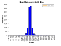
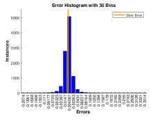
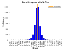
Figure 1: Histograms of errors for the learned network ${\cal N}$. ${\cal N}$ was applied to $10^{4}$ samples randomly selected from the $10^{4}N_{par}$ cases used for learning. Histograms are shown for $m_{1},m_{2},m_{3}$, the three coordinates of $m$. $m_{1},m_{2},m_{3}$ were rescaled to normalized values in $[0,1]$ to facilitate comparison.

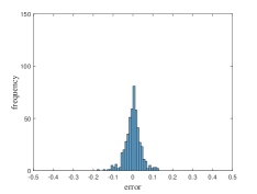
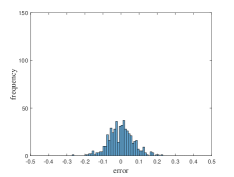
Figure 2: Errors for the reconstruction of $m_{1}$, the first coordinate of $m$, normalized to $[0,1]$ following three different methods: by application of ${\cal N}$, by minimization over ${\cal S}$, and minimization over ${\cal S}_{0}$. These errors are for a set of $500$ draws of $m$ and random forcing vectors that were not used in the learning step. Note that the neural network ${\cal N}$ reconstructs all coordinates of $m$ simultaneously. Error histograms in reconstructing $m_{2},m_{3}$ present a similar profile and are not shown.

	average error	load time	run time
${\cal N}$	0.015	0.018	0.049
${\cal S}$	0.028	3.5	47
${\cal S}_{0}$	0.055	0.053	0.19

Figure 3: For the same 500 instances of the data for the inverse problem as in figure 2: column 1, average error (absolute value) for $m_{1}$ normalized to $[0,1]$ following three different methods: by application of ${\cal N}$, by minimization over ${\cal S}$, and minimization over ${\cal S}_{0}$. Column 2: load time of file containing ${\cal N}$, ${\cal S}$, ${\cal S}_{0}$, in seconds. Column 3: cumulative run time for these 500 instances, in seconds.

	average error for ${\cal T}_{q^{\prime},0}$	average error for ${\cal T}_{q^{\prime},noisy}$
${\cal N}$	0.0178	0.0286
${\cal S}$	0.0277	0.0280
${\cal S}_{0}$	0.0491	0.0488

Figure 4: Column 1: average error over the test set ${\cal T}_{q^{\prime},0}$ for the reconstruction of $m_{1}$ normalized to $[0,1]$ following three methods: by application of ${\cal N}$, by minimization over ${\cal S}$, and minimization over ${\cal S}_{0}$. Column 2: same quantities for the test set ${\cal T}_{q^{\prime},noisy}$.

Funding
This work was supported by Simons Foundation Collaboration Grant [351025].

References

- [1] G. Alessandrini and L. Rondi. Determining a sound-soft polyhedral scatterer by a single far-field measurement. Proceedings of the American Mathematical Society, 133(6):1685–1691, 2005.
- [2] A. Aspri, E. Beretta, and A. L. Mazzucato. Dislocations in a layered elastic medium with applications to fault detection. preprint arXiv:2004.00321v1, 2020.
- [3] A. Aspri, E. Beretta, A. L. Mazzucato, and V. Maarten. Analysis of a model of elastic dislocations in geophysics. Archive for Rational Mechanics and Analysis, 236(1):71–111, 2020.
- [4] B. Calderhead. A general construction for parallelizing metropolis- hastings algorithms. Proceedings of the National Academy of Sciences, 111(49):17408–17413, 2014.
- [5] D. L. Colton, R. Kress, and R. Kress. Inverse acoustic and electromagnetic scattering theory, volume 93. Springer, 2013.
- [6] M. Costabel. Boundary integral operators on lipschitz domains: elementary results. SIAM Journal on Mathematical Analysis, 19(3):613–626, 1988.
- [7] C. Dascalu, I. R. Ionescu, and M. Campillo. Fault finiteness and initiation of dynamic shear instability. Earth and Planetary Science Letters, 177(3):163–176, 2000.
- [8] T. De Ryck, S. Lanthaler, and S. Mishra. On the approximation of functions by tanh neural networks. Neural Networks, 143:732–750, 2021.
- [9] I. R. Ionescu and D. Volkov. An inverse problem for the recovery of active faults from surface observations. Inverse problems, 22(6):2103, 2006.
- [10] I. R. Ionescu and D. Volkov. Earth surface effects on active faults: An eigenvalue asymptotic analysis. Journal of Computational and Applied Mathematics, 220(1):143–162, 2008.
- [11] T. Kato. Perturbation theory for linear operators, volume 132. Springer Science & Business Media, 2013.
- [12] M. F. Møller. A scaled conjugate gradient algorithm for fast supervised learning. Neural networks, 6(4):525–533, 1993.
- [13] Y. Okada. Internal deformation due to shear and tensile faults in a half-space. Bulletin of the Seismological Society of America, vol. 82 no. 2:1018–1040, 1992.
- [14] R. Potthast. Fréchet differentiability of boundary integral operators in inverse acoustic scattering. Inverse Problems, 10(2):431, 1994.
- [15] Z. Shen, H. Yang, and S. Zhang. Neural network approximation: Three hidden layers are enough. Neural Networks, 141:160–173, 2021.
- [16] F. Triki and D. Volkov. Stability estimates for the fault inverse problem. Inverse problems, 35(7), 2019.
- [17] D. Volkov. A double layer surface traction free green’s tensor. SIAM Journal on Applied Mathematics, 69(5):1438–1456, 2009.
- [18] D. Volkov. A parallel sampling algorithm for some nonlinear inverse problems. IMA Journal of Applied Mathematics, 2022. https://doi.org/10.1093/imamat/hxac003.
- [19] D. Volkov. A stochastic algorithm for fault inverse problems in elastic half space with proof of convergence. Journal of Computational Mathematics, in press.
- [20] D. Volkov and Y. Jiang. Stability properties of a crack inverse problem in half space. Mathematical methods in the applied sciences, 44(14):11498–11513, 2021.
- [21] D. Volkov and J. C. Sandiumenge. A stochastic approach to reconstruction of faults in elastic half space. Inverse Problems & Imaging, 13(3):479–511, 2019.
- [22] D. Volkov, C. Voisin, and I. Ionescu. Reconstruction of faults in elastic half space from surface measurements. Inverse Problems, 33(5), 2017.
- [23] D. Volkov, C. Voisin, and I. I.R. Determining fault geometries from surface displacements. Pure and Applied Geophysics, 174(4):1659–1678, 2017.
- [24] D. Yarotsky. Error bounds for approximations with deep relu networks. Neural Networks, 94:103–114, 2017.