On Supervised Feature Selection from High Dimensional Feature Spaces

Abstract

The application of machine learning to image and video data often yields a high dimensional feature space. Effective feature selection techniques identify a discriminant feature subspace that lowers computational and modeling costs with little performance degradation. A novel supervised feature selection methodology is proposed for machine learning decisions in this work. The resulting tests are called the discriminant feature test (DFT) and the relevant feature test (RFT) for the classification and regression problems, respectively. The DFT and RFT procedures are described in detail. Furthermore, we compare the effectiveness of DFT and RFT with several classic feature selection methods. To this end, we use deep features obtained by LeNet-5 for MNIST and Fashion-MNIST datasets as illustrative examples. Other datasets with handcrafted and gene expressions features are also included for performance evaluation. It is shown by experimental results that DFT and RFT can select a lower dimensional feature subspace distinctly and robustly while maintaining high decision performance.

1 Introduction

Traditional machine learning algorithms are susceptible to the curse of feature dimensionality [1]. Their computational complexity increases with high dimensional features. Redundant features may not be helpful in discriminating classes or reducing regression error, and they should be removed. Sometimes, redundant features may even produce negative effects as their number grows. their detrimental impact should be minimized or controlled. To deal with these problems, feature selection techniques [2, 3, 4] are commonly applied as a data pre-processing step or part of the data analysis to simplify the complexity of the model. Feature selection techniques involve the identification of a subspace of discriminant features from the input, which describe the input data efficiently, reduce effects from noise or irrelevant features, and provide good prediction results [5].

For machine learning with image/video data, the deep learning technology, which adopts a pre-defined network architecture and optimizes the network parameters using an end-to-end optimization procedure, is dominating nowadays. Yet, an alternative that returns to the traditional pattern recognition paradigm based on feature extraction and classification two modules in cascade has also been studied, e.g., [6, 7, 8, 9, 10, 11, 12, 13, 14, 15]. The feature extraction module contains two steps: unsupervised representation learning and supervised feature selection. Examples of unsupervised representation learning include multi-stage Saab [10] and Saak transforms [6]. Here, we focus on the second step; namely, supervised feature selection from a high dimensional feature space.

Inspired by information theory and the decision tree, a novel supervised feature selection method is proposed in this work. The resulting tests are called the discriminant feature test (DFT) and the relevant feature test (RFT), respectively, for the classification and regression problems. The DFT and RFT procedures are described in detail. We compare the effectiveness of DFT and RFT with several classic feature selection methods. Experimental results show that DFT and RFT can select a significantly lower dimensional feature subspace distinctly and robustly while maintaining high decision performance.

The rest of this paper is organized as follows. Related previous work is reviewed in Sec. 2. DFT and RFT are presented in Sec. 3. Experimental results are shown in Sec. 4. Finally, concluding remarks are given in Sec. 5.

2 Review of Previous Work

Feature selection methods can be categorized into unsupervised [16, 17, 18, 19], semi-supervised [20, 21], and supervised [22] three types. Unsupervised methods focus on the statistics of input features while ignoring the target class or value. Straightforward unsupervised methods can be fast, e.g., removing redundant features using correlation, removing features of low variance. However, their power is limited and less effective than supervised methods. More advanced unsupervised methods adopt clustering. Examples include [23, 24, 25]. Their complexity is higher, their behavior is not well understood, and their performance is not easy to evaluate systematically. Overall, this is an open research field.

Existing semi-supervised and supervised feature selection methods can be classified into wrapper, filter and embedded three classes [20]. Wrapper methods [26] create multiple models with different subsets of input features and select the model containing the features that yield the best performance. One example is recursive feature elimination (RFE) [27]. This process can be computationally expensive. Filter methods involve evaluating the relationship between input and target variables using statistics and selecting those variables that have the strongest relation with the target ones. One example is the analysis of variance (ANOVA) [28]. This approach is computationally efficient with robust performance. Another example is feature selection based on linear discriminant analysis (LDA). It finds the most separable projection directions. The objective function of LDA is used to select discriminant features from the existing feature dimensions by measuring the ratio between the between-class scatter matrix and the within-class scatter matrix. It can be generalized from the 2-class problem to the multi-class problem. Embedded methods perform feature selection in the process of training and are usually specific to a single learner. One example is “feature importance" (FI) obtained from the training process of the XGBoost classifier/regressor [29], which is also known as “feature selection from model" (SFM).

Inspired by information theory and the decision tree, a novel supervised feature selection methodology is proposed in this work. The resulting tests are called the discriminant feature test (DFT) and the relevant feature test (RFT) for classification and regression tasks, respectively. Our proposed methods belong to the filter methods, which give a score to each dimension and select features based on feature ranking. The scores are measured by the weighted entropy and the weighted MSE for DFT and RFT, which reflect the discriminant power and relevance degree to classification and regression targets, respectively.

To demonstrate the power of DFT and RFT, we conduct performance benchmarking between DFT/RFT, ANOVA and FI from XGBoost in the experimental section. To this end, we use deep features obtained by LeNet-5 for MNIST and Fashion-MNIST datasets as illustrative examples. Other datasets with handcrafted features and gene expressions features are also used for performance benchmarking. Comparison with the minimal-redundancy-maximal-relevance (mRMR) criterion [30, 31], which is a more advanced feature selection method, is also conducted. It is shown by experimental results that DFT and RFT can select a lower dimensional feature subspace distinctly and robustly while maintaining high decision performance.

Figure 1: An overview of the proposed feature selection methods: DFT and RFT. For the $i$-th feature, DFT measures the class distribution in $S^{i}_{L}$ and $S^{i}_{R}$ to compute the weighted entropy as the DFT loss, while RFT measures the weighted estimated regression MSE in both sets as the RFT loss.

3 Proposed Feature Selection Methods

Being motivated by the feature selection process in the decision tree classifier, we propose two feature selection methods, DFT and RFT, in this section as illustrated in Fig. 1. They will be detailed in Sec. 3.1 and Sec. 3.2, respectively. Finally, robustness of DFT and RFT will be discussed in Sec. 3.3.

3.1 Discriminant Feature Test (DFT)

Consider a classification problem with $N$ data samples, $P$ features and $C$ classes. Let $f^{i}$, $1\leq i\leq P$, be a feature dimension and its minimum and maximum are $f_{\min}^{i}$ and $f_{\max}^{i}$, respectively. DFT is used to measure the discriminant power of each feature dimension out of a $P$-dimensional feature space independently. If feature $f^{i}$ is a discriminant one, we expect data samples projected to it should be classified more easily. To check it, one idea is to partition $[f_{\min}^{i},f_{\max}^{i}]$ into $M$ nonoverlapping subintervals and adopt the maximum likelihood rule to assign the class label to samples inside each subinterval. Then, we can compute the percentage of correct predictions. The higher the prediction accuracy, the higher the discriminant power. Although prediction accuracy may serve as an indicator for purity, it does not tell the distribution of the remaining $C-1$ classes if $C>2$. Thus, it is desired to consider other purity measures.

In our design, we use the weighted entropy of the left and right subsets as the DFT loss to measure the discriminant power of each dimension. The reason of choosing the weighted entropy as the cost is that it considers the probability distribution of all classes instead of the maximum likelihood rule in prediction accuracy as stated above. A lower entropy value is obtained from a more biased distribution of classes, indicating the subinterval is dominated by fewer classes.

By following the practice of a binary decision tree, we consider the case, $M=2$, as shown in the left subfigure of Fig. 1, where $f_{t}^{i}$ denotes the threshold position of two sub-intervals. If a sample with its $i$th dimension, $x^{i}_{n}<f_{t}^{i}$, it goes to the subset associated with the left subinterval. Otherwise, it will go to the subset associated with the right subinterval. Formally, the procedure of DFT consists of three steps for each dimension as detailed below.

3.1.1 Training Sample Partitioning

For the $i$th feature, $f^{i}$, we need to search for the optimal threshold, $f^{i}_{op}$, between $[f_{\min}^{i},f_{\max}^{i}]$ and partition training samples into two subsets $S^{i}_{L}$ and $S^{i}_{R}$ via

$$\mbox{if}\,x^{i}_{n}<f^{i}_{op},\;x_{n}\,\epsilon\,S^{i}_{L};\;\;$$ (1)

$$\mbox{otherwise},\;x_{n}\,\epsilon\,S^{i}_{R},$$ (2)

where $x^{i}_{n}$ represents the $i$-th feature of the $n$-th training sample $x_{n}$, and $f^{i}_{op}$ is selected automatically to optimize a certain purity measure. To limit the search space of $f^{i}_{op}$, we partition the entire feature range, $[f_{\min}^{i},f_{\max}^{i}]$, into $B$ uniform segments and search the optimal threshold among the following $B-1$ candidates:

$$f_{b}^{i}=f_{\min}^{i}+\frac{b}{B}[f_{\max}^{i}-f_{\min}^{i}],\quad b=1,\cdots,B-1,$$ (3)

where $B=2^{j}$, $j=1,2\cdots$, is examined in Sec. 3.3.

3.1.2 DFT Loss Measured by Entropy

Samples of different classes belong to $S^{i}_{L}$ or $S^{i}_{R}$. Without loss of generality, the following discussion is based on the assumption that each class has the same number of samples in the full training set; namely $S^{i}_{L}\cup S^{i}_{R}$. To measure the purity of subset $S^{i}_{L}$ corresponding to the partition point $f^{i}_{t}$, we use the following entropy metric:

$$H^{i}_{L,t}=-\sum_{c=1}^{C}p^{i}_{L,c}log(p^{i}_{L,c}),$$ (4)

where $p^{i}_{L,c}$ is the probability of class $c$ in $S^{i}_{L}$. Similarly, we can compute entropy $H^{i}_{R,t}$ for subset $S^{i}_{R}$. Then, the entropy of the full training set against partition $f^{i}_{t}$ is the weighted average of $H_{L,t}$ and $H_{R,t}$ in form of

$$H^{i}_{t}=\frac{N^{i}_{L,t}H^{i}_{L,t}+N^{i}_{R,t}H^{i}_{R,t}}{N},$$ (5)

where $N^{i}_{L,t}$ and $N^{i}_{R,t}$ are the sample numbers in subsets $S^{i}_{L}$ and $S^{i}_{R}$, respectively, and $N=N^{i}_{L,t}+N^{i}_{R,t}$ is the total number of training samples. The optimized entropy $H^{i}_{op}$ for the $i$-th feature is given by

$$H^{i}_{op}=\min_{t\epsilon T}H^{i}_{t},$$ (6)

where $T$ indicates the set of partition points.

3.1.3 Feature Selection Based on Optimized Loss

We conduct search for optimized entropy values, $H^{i}_{op}$, of all feature dimensions, $f^{i}$, $1\leq i\leq P$ and order the values of $H^{i}_{op}$ from the smallest to the largest ones. The lower the $H^{i}_{op}$ value, the more discriminant the $i$th-dimensional feature, $f^{i}$. Then, we select the top $K$ features with the lowest entropy values as discriminant features. To choose the value of $K$ with little ambiguity, it is critical the rank-ordered curve of $H^{i}_{op}$ should satisfy one important criterion. That is, it should have a distinct and narrow elbow region. We will show that this is indeed the case in Sec. 4.

3.2 Relevant Feature Test (RFT)

For regression tasks, the mapping between an input feature and a target scalar function can be more efficiently built if the feature dimension has the ability to separate samples into segments with smaller variances. This is because the regressor can use the mean of each segment as the target value, and its corresponding variance indicates the prediction mean squared-error (MSE) of the segment. Motivated by this observation and the binary decision tree, RFT partitions a feature dimension into the left and right two subintervals and evaluates the total MSE from them. We use this approximation error as the RFT loss function. The smaller the RFT loss, the better the feature dimension. Again, the RFT loss depends on the threshold $f_{t}^{i}$. The process of selecting more powerful feature dimensions for regression is named Relevant Feature Test (RFT). Similar to DFT, RFT has three steps. They are elaborated below. Here, we adopt the same notations as those in Sec. 3.1.

3.2.1 Training Sample Partitioning

By following the first step in DFT, we search for the optimal threshold, $f^{i}_{op}$, between $[f_{\min}^{i},f_{\max}^{i}]$ and partition training samples into two subsets $S^{i}_{L}$ and $S^{i}_{R}$ for the $i$th feature, $f^{i}$. Again, we partition the feature range, $[f_{\min}^{i},f_{\max}^{i}]$, into $B$ uniform segments and search the optimal threshold among the following $B-1$ candidates as given in Eq. (3).

3.2.2 RFT Loss Measured by Estimated Regression MSE

We use $y$ to denote the regression target value. For the $i$th feature dimension, $f^{i}$, we partition the sample space into two disjoint ones $S^{i}_{L}$ and $S^{i}_{R}$. Let $y^{i}_{L}$ and $y^{i}_{R}$ be the mean of target values in $S^{i}_{L}$ and $S^{i}_{R}$, and we use $y^{i}_{L}$ and $y^{i}_{R}$ as the estimated regression value of all samples in $S^{i}_{L}$ and $S^{i}_{R}$, respectively. Then, the RFT loss is defined as the sum of estimated regression MSEs of $S^{i}_{L}$ and $S^{i}_{R}$. Mathematically, we have

$$R^{i}_{t}=\frac{N^{i}_{L,t}R^{i}_{L,t}+N^{i}_{R,t}R^{i}_{R,t}}{N},$$ (7)

where $N=N^{i}_{L,t}+N^{i}_{R,t}$, $N^{i}_{L,t}$, $N^{i}_{R,t}$, $R^{i}_{L,t}$ and $R^{i}_{R,t}$ denote the sample numbers and the estimated regression MSEs in subsets $S^{i}_{L}$ and $S^{i}_{R}$, respectively. Feature $f^{i}$ is characterized by its optimized estimated regression MSE over the set, $T$, of candidate partition points:

$$R^{i}_{op}=\min_{t\epsilon T}R^{i}_{t}.$$ (8)

3.2.3 Feature Selection Based on Optimized Loss

We order the optimized estimated regression MSE value, $R^{i}_{op}$ across all feature dimensions, $f^{i}$, $1\leq i\leq P$, from the smallest to the largest ones. The lower the $R^{i}_{op}$ value, the more relevant the $i$th-dimensional feature, $f^{i}$. Afterwards, we select the top $K$ features with the lowest estimated regression MSE values as relevant features.

3.3 Robustness Against Bin Numbers

For smooth DFT/RFT loss curves with a sufficiently large bin number (say, $B\geq 16$), the optimized loss value does not vary much by increasing $B$ furthermore as shown in Fig. 2. Figs. 2(a) and (b) show the DFT and RFT loss functions for an exemplary feature, $f^{i}$, under two binning schemes; i.e., $B=16$ and $B=64$, respectively. We see that the binning $B=16$ is fine enough to locate the optimal partition $f^{i}_{op}$. If $B=2^{j}$, $j=1,2,\cdots$, the set of partition points in a small $B$ value is a subset of those of a larger $B$ value. Generally, we have the following observations. The difference of the DFT/RFT loss between adjacent candidate points changes smoothly. Since the global minimum has a flat bottom, the loss function is low for a range of partition thresholds. The feature will achieve a similar loss level with multiple binning schemes. For example, Fig. 2(a) shows that $B=16$ reaches the global minimum at $f^{i}=5.21$ while $B=64$ reaches the global minimum at $f^{i}=5.78$. The difference is about 3% of the full dynamic range of $f^{i}$. Similar characteristics are observed for all feature dimensions in DFT/RFT, indicating the robustness of DFT/RFT. For lower computational complexity, we typically choose $B=16$ or $B=32$.

(a)

(b)

Figure 2: Comparison of two binning schemes with $B=16$ and $B=64$: (a) DFT and (b) RFT.

4 Experimental Results

4.1 Image Datasets with High Dimensional Feature Space

To demonstrate the power of DFT and RFT, we consider several classical datasets. They include MNIST [32], Fashion-MNIST [33], the Multiple Features (MultiFeat) dataset, the Arrhythmia (ARR) dataset [34] from the UCI machine learning archive [35], and the Colon cancer dataset [36]. The latter three are used to measure DFT in the classification problem setting.

Dataset-1: MNIST and Fashion-MNIST. Both datasets contain grayscale images of resolution $28\times 28$, with 60K training and 10K test images. MNIST has 10 classes of hand-written digits (from 0 to 9) while Fashion-MNIST has 10 classes of fashion products. In order to get deep features for each dataset, we train the LeNet-5 network [32] for the two corresponding classification problems and adopt the 400-D feature vector before the two FC layers as raw features to evaluate several feature selection methods. Besides original clean training images, we add additive zero-mean Gaussian noise with different standard deviation values to evaluate the robustness of feature selection methods against noisy data. The LeNet-5 network is re-trained for these noisy images and the corresponding deep features are extracted. For the performance benchmarking purpose, we list the test classification accuracy of the trained LeNet-5 for MNIST and Fashion-MNIST in Table 1 to illustrate the quality of the deep features.

Table 1: Classification accuracy (%) of LeNet-5 on MNIST and Fashion-MNIST.

	Clean	Noisy
MNIST	99.18	98.85
Fashion-MNIST	90.19	86.95

Dataset-2: MultiFeat [37, 38, 39]. This dataset contains features of hand-written digits (from 0 to 9) extracted from a collection of Dutch utility maps  [35], including 649 dimensional features for 200 images per class. Different from the deep features in Dataset-1, the 649 features are extracted from six perspectives such as Fourier coefficients of character shapes and morphological features. Since the number of samples is small, we use 10-fold cross-validation and compute the mean accuracy to evaluate the classification performance.

Dataset-3: Colon. This gene expression dataset contains 62 samples with 2000 features each. It has a binary classification label; namely, the normal tissue or the cancerous tissue. There are 22 normal tissue and 40 cancer tissue samples. Considering its small sample size, we use the leave-one-out validation to get the classification predictions for each sample.

Dataset-4: ARR. This cardiac arrhythmia dataset has binary labels for 237 normal and 183 abnormal samples. Each sample contains 278 features. The 10-fold cross-validation is adopted to evaluate the classification performance.

4.2 DFT for Classification Problems

We compare effectiveness of four feature selection methods: 1) F scores from ANOVA (ANOVA F Scores), 2) absolute correlation coefficient w.r.t the class labels (Abs. Corr. Coeff.), 3) feature importance (Feat. Imp.) from a pre-trained XGBoost classifier, and 4) DFT. We adopt four classifiers to validate the classification performance. They are the Logistic Regression (LR) classifier [40], the Support Vector Machine (SVM) classifier [41], the Random Forest (RF) classifier [42], and the XGBoost classifier [29]. We have the following two observations.

4.2.1 DFT offers an obvious elbow point

Fig. 3 compares the ranked scores of four feature selection methods on Fashion-MNIST dataset. The lower DFT loss, the higher importance of a feature. The other three have a reversed relation, namely, the higher the score, the higher the importance. Thus, we search for the elbow point for DFT but the knee point for the other methods. Clearly, the feature importance curve from the pre-trained XGBoost classifier has a clearer knee point and the DFT curve has a more obvious elbow point. In contrast, ANOVA and correlation-coefficient-based methods are not as effective in selecting discriminant features since their knee points are less obvious.

Figure 3: Comparison of distinct feature selection capability among four feature selection methods for the classification task on the Fashion-MNIST dataset.

4.2.2 Features selected by DFT achieves comparable and stable classification performance

Tables 2 - 5 summarize the classification accuracy using four classifiers at two reduced dimensions selected by the DFT loss curve based on early and late elbow points on Dataset-1. The RBF kernel is used for SVM. We see that DFT can achieve comparable (or even the best) performance among the four methods at the same selected feature dimension. The accuracy gap between the late elbow point and the full feature set (400-D) is very small. They are 0.62% and 0.94% using XGBoost classifier for clean MNIST and Fashion-MNIST, respectively. The late elbow point only uses 25-35% of the full feature set. The gaps in classification accuracy on noisy images are 0.58% and 1.6% for MNIST and Fashion-MNIST, respectively, indicating the robustness of the DFT feature selection method against input perturbation.

We also show the classification performance on the Colon dataset using LR and SVM in Table 6, where the linear kernel is used in SVM. DFT has the minimum or a comparable number of errors in leave-one-out validation. Furthermore, DFT can always achieve fewer errors as compared to the setting of using all 2000 features.

Table 2: Comparison of classification performance (%) on Clean MNIST between different feature selection methods.

Selected Dimension	Method	LR	SVM	RF	XGBoost
	ANOVA	94.21	95.07	95.77	96.58
Early Elbow Point	Corr.	88.73	92.47	94.04	95.11
(30-D)	Feat. imp.	92.61	93.55	94.89	95.71
	DFT (Ours)	94.49	95.45	96.29	96.92
	ANOVA	98.24	98.22	97.98	98.66
Late Elbow Point	Corr.	97.61	97.78	97.35	98.57
(100-D)	Feat. imp.	98.24	98.15	98.18	98.78
	DFT (Ours)	97.93	97.83	97.81	98.52
Full Set (400-D)		98.89	98.77	98.61	99.14

Table 3: Comparison of classification performance (%) on Noisy MNIST between different feature selection methods.

Selected Dimension	Method	LR	SVM	RF	XGBoost
	ANOVA	94.22	94.62	95.60	96.04
Early Elbow Point	Corr.	90.97	93.06	93.64	95.21
(40-D)	Feat. imp.	92.59	93.35	94.48	95.34
	DFT (Ours)	94.03	95.22	95.78	96.59
	ANOVA	96.81	96.87	97.16	97.99
Late Elbow Point	Corr.	96.87	97.13	96.83	97.93
(100-D)	Feat. imp.	97.22	97.2	97.36	97.97
	DFT (Ours)	97.08	97.36	97.49	98.18
Full Set (400-D)		98.04	98.17	98.15	98.76

Table 4: Comparison of classification performance (%) on Clean Fashion-MNIST between different feature selection methods.

Selected Dimension	Method	LR	SVM	RF	XGBoost
	ANOVA	78.85	80.44	83.33	83.11
Early Elbow Point	Corr.	76.57	80.16	82.69	83.04
(30-D)	Feat. imp.	78.96	80.49	82.99	82.96
	DFT (Ours)	79.59	81.48	84.03	84.09
	ANOVA	87.06	86.61	87.69	89.08
Late Elbow Point	Corr.	86.99	86.96	87.36	88.81
(150-D)	Feat. imp.	87.47	87.62	88.28	89.33
	DFT (Ours)	87.60	87.02	87.71	89.13
Full Set (400-D)		89.05	88.18	88.74	90.07

Table 5: Comparison of classification performance (%) on Noisy Fashion-MNIST between different feature selection methods.

Selected Dimension	Method	LR	SVM	RF	XGBoost
	ANOVA	75.35	76.41	77.94	78.62
Early Elbow Point	Corr.	75.55	77.94	79.22	80.50
(40-D)	Feat. imp.	75.73	77.1	78.06	78.63
	DFT (Ours)	76.35	77.92	79.23	79.69
	ANOVA	81.84	81.98	82.42	84.10
Late Elbow Point	Corr.	82.26	82.9	82.59	84.72
(150-D)	Feat. imp.	83.19	83.43	83.54	84.91
	DFT (Ours)	82.08	82.40	82.61	84.31
Full Set (400-D)		84.35	84.24	84.23	85.91

Table 6: Comparison of number of errors on Colon cancer dataset between different feature selection methods.

Classifier	Method	Selected Dimension						Full Set
		5	10	20	50	80	100	2000-D
LR	ANOVA	6	9	10	10	7	7	10
	Corr.	6	9	10	10	7	7
	Feat. Imp.	8	6	5	5	9	9
	DFT (Ours)	6	7	9	8	7	7
SVM	ANOVA	6	7	7	9	8	9	9
	Corr.	6	7	7	9	8	9
	Feat. Imp.	6	6	5	6	9	8
	DFT (Ours)	6	6	8	8	6	6

4.2.3 Comparison between DFT and mRMR

The minimal-redundancy-maximal-relevance (mRMR) [30, 31] aims at finding a feature set with high relevance to the class while keeping the selected features with small redundancy, leading to an efficient but effective subset of features. It combines constraints measured by the mutual information of both relevance to the class and redundancy between selected features and treats it as an optimization problem. In this experiment, we compare DFT with mRMR using its incremental selection scheme.

Figs. 4-6 compare the performance of mRMR and DFT on MultiFeat, Colon and ARR datasets with SVM and XGBoost classifiers. For MultiFeat and Colon, DFT can achieve very competitive performance with mRMR. Specifically, the most discriminant feature of MultiFeat selected by DFT is identical to the first feature selected by mRMR. The error rate with the top 5 features selected by mRMR is smaller than that of DFT. Yet, the performance gap is substantially narrowed after selecting more than 10 features out of the total 649 features. Overall, the error rate of DFT and mRMR converges at similar reduced dimensions, as shown in Figs. 4 and 6. On the other hand, the error rate of DFT on the ARR dataset is much lower than that of mRMR, with around 2.5% and 5% gap at 100 selected features for SVM and XGBoost, respectively, as shown in Fig. 6.

4.2.4 DFT requires less running time

We compare time efficiency of DFT, ANOVA, mRMR and feature importance from the XGBoost model. Table 7 summarizes the running time for MultiFeat, Colon and ARR datasets. All methods are run on the same CPU. The pre-trained XGBoost classifier uses the maximum depth of one with 300 trees. For filter methods such as ANOVA and DFT, the time is evaluated on all features without parallel computing. For mRMR, we set the maximum to 100 for incremental selection, which is smaller than the full feature set. ANOVA is the fastest and DFT method ranks the second on all three datasets. The running time of DFT with $B=16$ is about $\times 2.6$, $\times 7.3$ and $\times 23.1$ times faster than mRMR on MultiFeat, Colon and ARR, respectively. To further reduce the running time, our proposed DFT can be easily improved by adopting parallel computing since it processes each feature independently before the feature ranking.

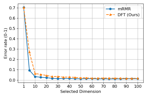
(a) SVM

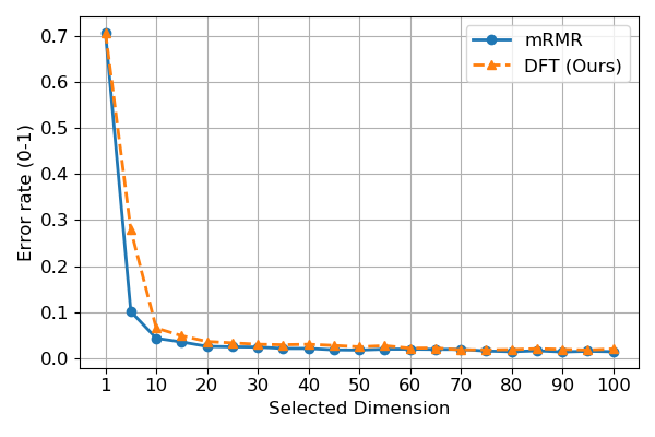
(b) XGBoost

Figure 4: Error rate comparison on the MultiFeat dataset between mRMR and DFT.

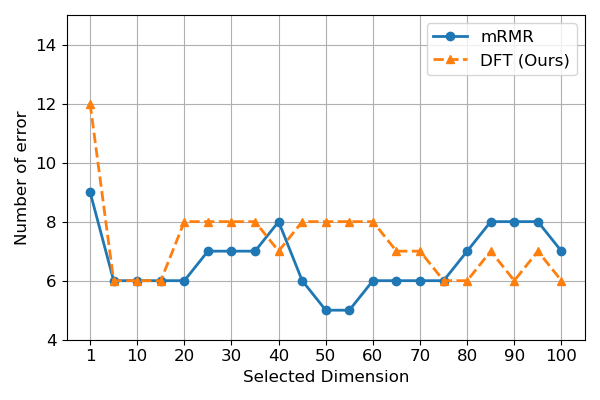
(a) SVM

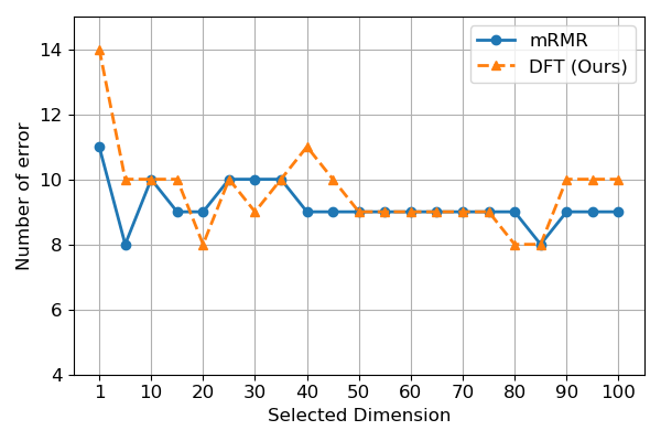
(b) XGBoost

Figure 5: Comparison of the number of errors on the Colon dataset between mRMR and DFT.

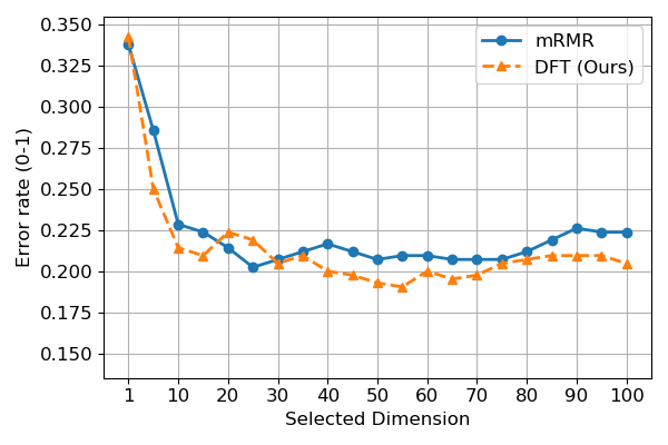
(a) SVM

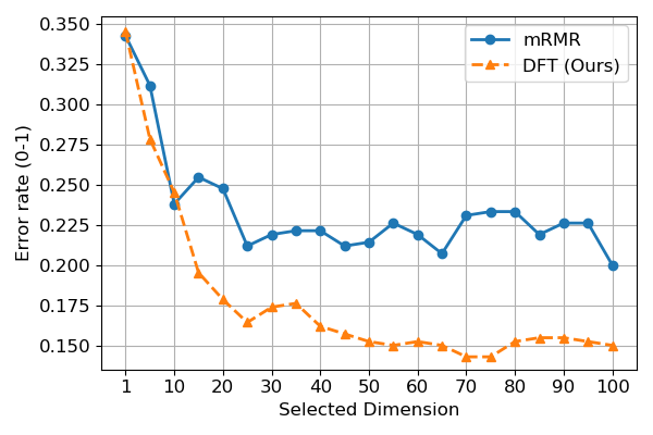
(b) XGBoost

Figure 6: Error rate comparison on the ARR dataset between mRMR and the DFT.

Table 7: Running time (sec.) comparison of different feature selection methods.

	ANOVA	Feat. Imp.	mRMR	DFT (B=8)	DFT (B=16)
MultiFeat	0.011	363.39	15.19	2.74	5.78
Colon	0.003	58.99	23.15	1.55	3.19
ARR	0.002	55.34	10.64	0.23	0.46

4.2.5 DFT with feature pre-processing

DFT assigns a score to each feature and selects a subset without any pre-processing. Yet, there might be correlation between features so that a redundant feature subset might be selected based on feature ranking [43]. Instead of adding redundancy measure to the DFT loss, we study the effect of combining DFT with feature pre-processing, such as PCA for feature decorrelation. We choose clean MNIST and Fashion-MNIST datasets as examples and perform PCA on the 400-D deep features without energy truncation. The DFT loss is calculated for each of 400 PCA-decorrelated features. After feature selection, the XGBoost classifier is applied. Fig. 7 compares the test accuracy under different selected dimensions for each setting. We see that PCA pre-processing improves the classification performance with the same selected dimension.

Furthermore, PCA pre-processing allows a smaller feature dimension for the same performance. For example, the accuracy on Fashion-MNIST saturates at around 15-D and 30-D with and without pre-processing, respectively. This can be explained by the energy compaction capability of PCA. Fig. 8 shows the histogram of energy ranking of the feature subset selected by DFT with and without PCA preprocessing. The raw features are first sorted by decreasing energy (variance) prior to feature selection. We see that the selected subset tends to gather in the first 20 to 50 principal components with PCA pre-preprocessing while the selected features are more widely distributed without PCA.

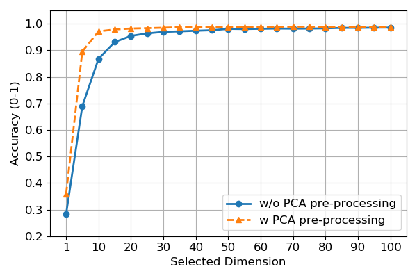
(a) MNIST

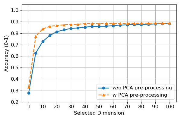
(b) Fashion-MNIST

Figure 7: Performance comparison of DFT feature selection with and without PCA feature pre-processing.

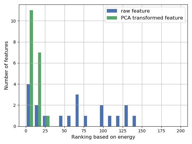
(a) Select 20 features

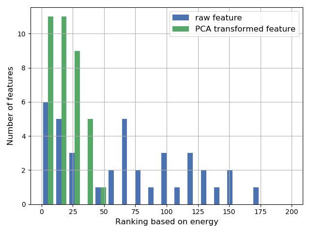
(b) Select 40 features

Figure 8: Histogram comparison of feature indices ranked by the energy with 20 and 40 selected feature numbers before and after PCA pre-processing. The smaller the ranking index in the x-axis, the higher the feature energy.

4.3 RFT for Regression Problems

We convert the discrete class labels arising from the classification problem to floating numbers so as to formulate a regression problem. We compare effectiveness of four feature selection methods: 1) variance (Var.), 2) absolute correlation coefficient w.r.t the regression target (Abs. Corr. Coeff.), 3) feature importance (Feat. Imp.) from a pre-trained XGBoost regressor (of 50 trees), and 4) RFT. Again, we can draw two conclusions.

4.3.1 RFT offers a more obvious elbow point

Fig. 9 compares the ranked scores for different feature selection methods. The lower RFT loss, the higher feature importance while the other three have a reversed relation. RFT has a more obvious elbow point than the knee points of Variance and correlation-based methods. The feature importance from the pre-trained XGBoost regressor saturates very fast (up to 24-D) and the difference among the remaining features is small. In contrast, RFT has a more distinct and reasonable elbow point, ensuring the performance after dimension reduction. A larger XGBoost model with more trees can help increase the feature number of higher importance. Yet, it is not clear what model size would be suitable for a particular regression problem.

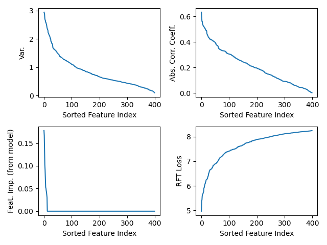
Figure 9: Comparison of relevant feature selection capability among four feature selection methods for the regression task on the Fashion-MNIST dataset.

4.3.2 Features selected by RFT achieves comparable and stable performance

Table 8 summarizes the regression MSE at two reduced dimensions selected by the RFT loss curves using early and late elbow points. The proposed RFT can achieve comparable (or even the best) performance among the four methods at the same selected feature dimension regardless whether the input images are clean or noisy. By employing only 25-37.5% of the total feature dimensions, the regression MSEs obtained by the late elbow point of RFT are 20-30% and 5-10% higher than those of the full feature set for MNIST and Fashion MNIST, respectively. This demonstrates the effectiveness of the RFT feature selection method.

Table 8: Regression MSE comparison for MNIST (clean/noisy) images with features selected by four methods.

Method	Early Elbow Point	Late Elbow Point	Full Set
	30-D / 50-D	100-D / 100-D	400-D
Var.	1.45 / 1.23	0.90 / 0.99	0.70 / 0.83
Abs. Corr. Coeff.	1.43 / 1.37	0.90 / 1.06
Feat. Imp.	1.55 / 1.47	1.04 / 1.23
RFT (Ours)	1.37 / 1.36	0.91 / 1.04

Table 9: Regression MSE comparison for Fashion-MNIST (clean/noisy) images with features selected by four methods.

Method	Early Elbow Point	Late Elbow Point	Full Set
	30-D / 50-D	150-D / 150-D	400-D
Var.	2.08 / 1.98	1.46 / 1.73	1.35 / 1.62
Abs. Corr. Coeff.	1.95 / 1.96	1.49 / 1.75
Feat. Imp.	2.00 / 2.06	1.62 / 1.86
RFT (Ours)	1.97 / 1.96	1.48 / 1.73

5 Conclusion and Future Work

Two feature selection methods, DFT and RFT, were proposed for general classification and regression tasks in this work. As compared with other existing feature selection methods, DFT and RFT are effective in finding distinct feature subspaces by offering obvious elbow regions in DFT/RFT curves. They provide feature subspaces of significantly lower dimensions while maintaining near optimal classification/regression performance. They are computationally efficient. They are also robust to noisy input data.

Recently, there is an emerging research direction that targets at unsupervised representation learning [6, 7, 8, 11, 12, 14, 15]. Through this process, it is easy to get high dimensional feature spaces (say, 1000-D or higher). We plan to apply DFT/RFT to them and find discriminant/relevant feature subspaces for specific tasks.

References

- [1] P. Hammer, “Adaptive control processes: a guided tour (r. bellman),” 1962.
- [2] J. Tang, S. Alelyani, and H. Liu, “Feature selection for classification: A review,” Data classification: Algorithms and applications, p. 37, 2014.
- [3] J. Miao and L. Niu, “A survey on feature selection,” Procedia Computer Science, vol. 91, pp. 919–926, 2016.
- [4] B. Venkatesh and J. Anuradha, “A review of feature selection and its methods,” Cybernetics and Information Technologies, vol. 19, no. 1, pp. 3–26, 2019.
- [5] I. Guyon and A. Elisseeff, “An introduction to variable and feature selection,” Journal of machine learning research, vol. 3, no. Mar, pp. 1157–1182, 2003.
- [6] Y. Chen, Z. Xu, S. Cai, Y. Lang, and C.-C. J. Kuo, “A saak transform approach to efficient, scalable and robust handwritten digits recognition,” in 2018 Picture Coding Symposium (PCS), pp. 174–178, IEEE, 2018.
- [7] Y. Chen and C.-C. J. Kuo, “Pixelhop: A successive subspace learning (ssl) method for object recognition,” Journal of Visual Communication and Image Representation, vol. 70, p. 102749, 2020.
- [8] Y. Chen, M. Rouhsedaghat, S. You, R. Rao, and C.-C. J. Kuo, “Pixelhop++: A small successive-subspace-learning-based (ssl-based) model for image classification,” in 2020 IEEE International Conference on Image Processing (ICIP), pp. 3294–3298, IEEE, 2020.
- [9] C.-C. J. Kuo and Y. Chen, “On data-driven saak transform,” Journal of Visual Communication and Image Representation, vol. 50, pp. 237–246, 2018.
- [10] C.-C. J. Kuo, M. Zhang, S. Li, J. Duan, and Y. Chen, “Interpretable convolutional neural networks via feedforward design,” Journal of Visual Communication and Image Representation, 2019.
- [11] X. Liu, F. Xing, C. Yang, C.-C. J. Kuo, S. Babu, G. E. Fakhri, T. Jenkins, and J. Woo, “Voxelhop: Successive subspace learning for als disease classification using structural mri,” arXiv preprint arXiv:2101.05131, 2021.
- [12] A. Manimaran, T. Ramanathan, S. You, and C.-C. J. Kuo, “Visualization, discriminability and applications of interpretable saak features,” Journal of Visual Communication and Image Representation, vol. 66, p. 102699, 2020.
- [13] M. Rouhsedaghat, Y. Wang, X. Ge, S. Hu, S. You, and C.-C. J. Kuo, “Facehop: A light-weight low-resolution face gender classification method,” arXiv preprint arXiv:2007.09510, 2020.
- [14] M. Zhang, H. You, P. Kadam, S. Liu, and C.-C. J. Kuo, “Pointhop: An explainable machine learning method for point cloud classification,” IEEE Transactions on Multimedia, 2020.
- [15] M. Zhang, Y. Wang, P. Kadam, S. Liu, and C.-C. J. Kuo, “Pointhop++: A lightweight learning model on point sets for 3d classification,” in 2020 IEEE International Conference on Image Processing (ICIP), pp. 3319–3323, IEEE, 2020.
- [16] P. Mitra, C. Murthy, and S. K. Pal, “Unsupervised feature selection using feature similarity,” IEEE transactions on pattern analysis and machine intelligence, vol. 24, no. 3, pp. 301–312, 2002.
- [17] D. Cai, C. Zhang, and X. He, “Unsupervised feature selection for multi-cluster data,” in Proceedings of the 16th ACM SIGKDD international conference on Knowledge discovery and data mining, pp. 333–342, 2010.
- [18] M. Qian and C. Zhai, “Robust unsupervised feature selection,” in Twenty-third international joint conference on artificial intelligence, Citeseer, 2013.
- [19] S. Solorio-Fernández, J. A. Carrasco-Ochoa, and J. F. Martínez-Trinidad, “A review of unsupervised feature selection methods,” Artificial Intelligence Review, vol. 53, no. 2, pp. 907–948, 2020.
- [20] R. Sheikhpour, M. A. Sarram, S. Gharaghani, and M. A. Z. Chahooki, “A survey on semi-supervised feature selection methods,” Pattern Recognition, vol. 64, pp. 141–158, 2017.
- [21] Z. Zhao and H. Liu, “Semi-supervised feature selection via spectral analysis,” in Proceedings of the 2007 SIAM international conference on data mining, pp. 641–646, SIAM, 2007.
- [22] S. H. Huang, “Supervised feature selection: A tutorial.,” Artif. Intell. Res., vol. 4, no. 2, pp. 22–37, 2015.
- [23] D. D. Lee and H. S. Seung, “Learning the parts of objects by non-negative matrix factorization,” Nature, vol. 401, no. 6755, pp. 788–791, 1999.
- [24] J. A. Hartigan, “Direct clustering of a data matrix,” Journal of the american statistical association, vol. 67, no. 337, pp. 123–129, 1972.
- [25] C. C. Aggarwal, J. L. Wolf, P. S. Yu, C. Procopiuc, and J. S. Park, “Fast algorithms for projected clustering,” ACM SIGMoD Record, vol. 28, no. 2, pp. 61–72, 1999.
- [26] R. Kohavi and G. H. John, “Wrappers for feature subset selection,” Artificial intelligence, vol. 97, no. 1-2, pp. 273–324, 1997.
- [27] I. Guyon, J. Weston, S. Barnhill, and V. Vapnik, “Gene selection for cancer classification using support vector machines,” Machine learning, vol. 46, no. 1, pp. 389–422, 2002.
- [28] H. Scheffe, The analysis of variance, vol. 72. John Wiley & Sons, 1999.
- [29] T. Chen, T. He, M. Benesty, V. Khotilovich, Y. Tang, H. Cho, K. Chen, et al., “Xgboost: extreme gradient boosting,” R package version 0.4-2, vol. 1, no. 4, pp. 1–4, 2015.
- [30] H. Peng, F. Long, and C. Ding, “Feature selection based on mutual information criteria of max-dependency, max-relevance, and min-redundancy,” IEEE Transactions on pattern analysis and machine intelligence, vol. 27, no. 8, pp. 1226–1238, 2005.
- [31] C. Ding and H. Peng, “Minimum redundancy feature selection from microarray gene expression data,” Journal of bioinformatics and computational biology, vol. 3, no. 02, pp. 185–205, 2005.
- [32] Y. LeCun, L. Bottou, Y. Bengio, and P. Haffner, “Gradient-based learning applied to document recognition,” Proceedings of the IEEE, vol. 86, no. 11, pp. 2278–2324, 1998.
- [33] H. Xiao, K. Rasul, and R. Vollgraf, “Fashion-mnist: a novel image dataset for benchmarking machine learning algorithms,” arXiv preprint arXiv:1708.07747, 2017.
- [34] H. A. Guvenir, B. Acar, G. Demiroz, and A. Cekin, “A supervised machine learning algorithm for arrhythmia analysis,” in Computers in Cardiology 1997, pp. 433–436, IEEE, 1997.
- [35] D. Dua and C. Graff, “UCI machine learning repository,” 2017.
- [36] U. Alon, N. Barkai, D. A. Notterman, K. Gish, S. Ybarra, D. Mack, and A. J. Levine, “Broad patterns of gene expression revealed by clustering analysis of tumor and normal colon tissues probed by oligonucleotide arrays,” Proceedings of the National Academy of Sciences, vol. 96, no. 12, pp. 6745–6750, 1999.
- [37] M. van Breukelen, R. P. Duin, D. M. Tax, and J. Den Hartog, “Handwritten digit recognition by combined classifiers,” Kybernetika, vol. 34, no. 4, pp. 381–386, 1998.
- [38] M. Van Breukelen and R. P. Duin, “Neural network initialization by combined classifiers,” in Proceedings. Fourteenth International Conference on Pattern Recognition (Cat. No. 98EX170), vol. 1, pp. 215–218, IEEE, 1998.
- [39] A. Jain and D. Zongker, “Feature selection: Evaluation, application, and small sample performance,” IEEE transactions on pattern analysis and machine intelligence, vol. 19, no. 2, pp. 153–158, 1997.
- [40] D. R. Cox, “The regression analysis of binary sequences,” Journal of the Royal Statistical Society: Series B (Methodological), vol. 20, no. 2, pp. 215–232, 1958.
- [41] C. Cortes and V. Vapnik, “Support-vector networks,” Machine learning, vol. 20, no. 3, pp. 273–297, 1995.
- [42] L. Breiman, “Random forests,” Machine learning, vol. 45, no. 1, pp. 5–32, 2001.
- [43] G. Chandrashekar and F. Sahin, “A survey on feature selection methods,” Computers & Electrical Engineering, vol. 40, no. 1, pp. 16–28, 2014.