Super-resolution of generalized spikes and spectra of confluent Vandermonde matrices

Abstract

We study the problem of super-resolution of a linear combination of Dirac distributions and their derivatives on a one-dimensional circle from noisy Fourier measurements. Following numerous recent works on the subject, we consider the geometric setting of “partial clustering”, when some Diracs can be separated much below the Rayleigh limit. Under this assumption, we prove sharp asymptotic bounds for the smallest singular value of a corresponding rectangular confluent Vandermonde matrix with nodes on the unit circle. As a consequence, we derive matching lower and upper min-max error bounds for the above super-resolution problem, under the additional assumption of nodes belonging to a fixed grid.

Keywords— Super-resolution, Confluent Vandermonde matrix, Min-max error, Partial Fourier matrix, Sparse recovery, Smallest singular value, Dirac distributions, Decimation, ESPRIT

1 Introduction

1.1 Background

The problem of computional super-resolution (SR) is to recover the fine details of an unknown object from inaccurate measurments of inherently low resolution [1]. In recent years, there is much intrest in the problem of reconstructing a signal modelled by a linear combination of Dirac $\delta-$distributions (e.g. [2, 3, 4, 5, 6, 7, 8, 9, 10, 11] and references therein):

$$\mu(x)=\sum_{j=1}^{s}a_{j}\delta_{\xi_{j}}\quad a_{j}\in\mathbb{C},\;\delta_{\xi_{j}}=\delta(x-\xi_{j}),\ \xi_{j}\in(-\pi,\pi]$$ (1)

from noisy and bandlimited Fourier measurements:

$$y_{k}:=\hat{\mu}(k)+\eta_{k},\quad\hat{\mu}(k)=\langle\mu,e^{-ikx}\rangle,\quad k=0,1,...,M,\;|\eta_{k}|\leq\varepsilon.$$ (2)

For the model (1) we have $\hat{\mu}(k)=\sum_{j=1}^{s}a_{j}e^{ik\xi_{j}}$, and therefore the measurement vector $y=\{y_{k}\}_{k=0}^{M}$ can be expressed as

$$y=Va+\eta\in\mathbb{C}^{M+1}$$ (3)

where $V$ is the $(M+1)\times s$ Vandermonde matrix with the nodes on the unit circle:

$$V:=[e^{ik\xi_{j}}]_{k=0,...,M}^{j=1,...,s}.$$

In order to describe the stability of this inverse problem, suppose that the nodes $\xi_{j}$ belong to a grid of step size $\Delta$  and define the super-resolution factor (SRF) as $\frac{1}{(M\Delta)}$. Suppose that at most $\ell\leqslant s$ nodes form a ”cluster” of size $O(\Delta)$ (to be rigorously defined below). In the ”super-resolution regime” $SRF\gg 1$ [4, 5] showed that $\sigma_{\min}(V)$ scales like ${SRF}^{1-\ell}$ and consequently the worst-case reconstruction error rate of the coefficients of $\mu$ as in (1) from noisy measurements (2) is of the order ${SRF}^{2\ell-1}\varepsilon$. Despite the great amount of research devoted to the subject, there is currently no known tractable algorithm which provably achieves these min-max bounds for all signals of interest [3].

1.2 Our contributions

In this work we extend the methods and results of [4, 5] to the model

$$\mu=\sum_{j=1}^{s}a_{j}\delta_{\xi_{j}}+b_{j}\delta^{\prime}_{\xi_{j}},$$ (4)

where $\delta^{{}^{\prime}}$ is the distributional derivative of the Dirac delta. The Vandermonde matrix $V$ in (3) is replaced by the so-called confluent Vandermonde matrix $U$, which is defined (up to normalization) as:

$$U:=[e^{ik\xi_{j}}\ ke^{i(k-1)\xi_{j}}]_{k=0,...,M}^{j=1,...,s}.$$

Under the partial clustering assumptions, in Theorem 3.1 and 3.2 we prove a sharp lower and upper bounds for the smallest singular value of $U$ in the super-resolution regime, and show that it scales like ${SRF}^{1-2\ell}$. These bounds are proved by extending the decimation approach from [4] for the lower bound on $\sigma_{\min}(U)$, and by extending the finite difference approximation approach from [5] for the upper bound, further generalizing it to any node vector $\boldsymbol{\xi}$ satisfying the clustering assumptions. In addition, our proof technique for bounding the remainder part in the upper bound of the smallest singular value can be applied to gain a slight improvement in Proposition 2.10 in [5] by relaxing the conditions on $M,\Delta$.

As a consequence, in Theorem 3.3 we also obtain sharp min-max bounds of order ${SRF}^{4\ell-1}\varepsilon$ for the problem of sparse super-resolution of signals (4) on a grid by extending the corresponding technique from [4].

Also, we show numerically that the well-known ESPRIT method for exponential fitting (appropriately extended to handle higher multiplicities) is optimal, meaning that it attains the min-max error bounds we established in Theorem 3.3 for the recovered parameters of the signal (4).

In relation to prior work on the subject, in [12] the authors give a stability estimate for the more general model (5) with arbitrary fixed $n$, however assuming that the number of measurements $N+1$ equals the number of unknowns. Evaluating their estimate for our model and notation, their bound is of order ${\Delta}^{4\ell-1}{\varepsilon}^{\frac{1}{2}}$, while ours in the same case is ${\Delta}^{4\ell-1}{\varepsilon}$. In contrast, [13] established the bound in the super-resolution setting of a single cluster (and off-grid nodes) to be of order ${SRF}^{4\ell}\varepsilon$, while we derive the min-max rate ${SRF}^{4\ell-1}\varepsilon$.

1.3 Discussion

Naturally, our results and techniques pave the way to analyzing the general model

$$\mu=\sum_{j=1}^{s}\sum_{l=0}^{n}a_{j,l}\delta_{\xi_{j}}^{(l)}$$ (5)

in the clustered super-resolution regime. The applications of this model include modern sampling theory beyond the Nyquist rate, algebraic signal recovery, interpolation and multi-exponential analysis, to name a few (see [14, 15, 12, 16, 13, 17, 18] and references therein). At the same time, we believe that several recent developments on the basic model (1) can be utilized to the more general setting, as follows.

• Recently, [2] succeeded to establish sharp bounds for the entire spectrum of $V$ without requiring the entire node set to be contained in a small interval of length $\frac{\pi}{s^{2}}$. We believe that similar techniques could be applied to (4) in order to eliminate the above restriction.

• Optimal scaling of the constants in the above bounds for the spectrum of $V$ using harmonic analysis techniques has been investigated in [19], and it would be interesting to extend these methods to (5).

• While we obtain min-max rates for nodes on a grid, we expect to get similar rates for the ”off-grid” model as in [3], where the node locations can be any real number. Furthermore, it should be possible to establish component-wise bounds for the coefficients of different orders and for the nodes themselves, as done in [16, 12, 13] for the more restrictive geometric settings of the problem.

Going back to the model (1), confluent Vandermonde matrices appear naturally in the perturbation analysis of the nonlinear least squares problems [3, 13] for exponential fitting, and we expect our methods to be applicable in this context as well.

The paper is organized as follows. In section 2 we establish some notation. In section 3 we formulate the main results, which are proved in section 4. Finally, in section 5 we present numerical evidence confirming our bounds.

2 Preliminaries

2.1 Notation

Definition 2.1.

For $N\in\mathbb{N}$ and a vector $\boldsymbol{\xi}=(\xi_{1},...,\xi_{s})$ of pairwise distinct real nodes $\xi_{j}\in(-\pi,\pi]$, we define the rectangular $(2N+1)\times 2s$ confluent Vandermonde matrix $U_{N}(\boldsymbol{\xi})$ as

$$U_{N}(\boldsymbol{\xi}):=\frac{1}{\sqrt{2N}}\big{[}z^{k}_{j}\quad k{z_{j}}^{k-1}\big{]}^{j=1,\dots,s}_{k=0,\dots,2N}$$

s.t. $z_{j}=\exp(i\xi_{j})$.

The main subject of the paper is the scaling of the smallest singular value of $U_{N}$ when some of the nodes of $\boldsymbol{\xi}$ nearly collide (become very close to each other).

Definition 2.2 (wraparound distance).

For $t\in\mathbb{R}$, we denote

$$\|t\|_{\tilde{\mathbb{T}}}:=\big{|}\operatorname{Arg}\exp(it)\big{|}=\big{|}t\ \mod\ (-\pi,\pi]\big{|},$$

where $\operatorname{Arg}(z)$ is the principal value of the argument of $z\in\mathbb{C}\setminus\{0\}$, taking values in $(-\pi,\pi]$.

Definition 2.3 (minimal separation).

Given a vector of s distinct nodes $\boldsymbol{x}:=(x_{1},\dots,x_{s})$ with $x_{j}\in(-\pi,\pi]$, we define the minimal separation (in wraparound sense) as

$$\Delta:=\Delta(\boldsymbol{x})=\min_{i\neq j}\|x_{i}-x_{j}\|_{\tilde{\mathbb{T}}}\ .$$

Definition 2.4.

The node vector $\boldsymbol{x}=(x_{1},\dots,x_{s})\subset\big{(}-\frac{\pi}{2},\frac{\pi}{2}\big{]}$ is said to form a $(\Delta,\rho,s,\ell,\tau)$- clustered configuration for some $\Delta>0,2\leq\ell\leq s,\ell-1\leq\tau\leq\frac{\pi}{\Delta},$ and $\rho\geq 0$ if for each $x_{j}$ there exist at most $\ell$ distinct nodes

$$\boldsymbol{x}^{(j)}=\{x_{j,k}\}_{k=1,\dots,r_{j}}\subset\boldsymbol{x},\quad 1\leq r_{j}\leq\ell,\quad x_{j,1}\equiv x_{j},$$

such that the following conditions are satisfied:

1. For any $y\in\boldsymbol{x}^{(j)}\setminus\{x_{j}\}$, we have

   $$\Delta\leq\|y-x_{j}\|_{\tilde{\mathbb{T}}}\leq\tau\Delta.$$

2. For any $y\in\boldsymbol{x}\setminus\boldsymbol{x}^{(j)}$, we have

   $$\|y-x_{j}\|_{\tilde{\mathbb{T}}}\geq\rho.$$

Definition 2.5.

For $\Delta>0$ let $M=\big{\lfloor}\frac{\pi}{2\Delta}\big{\rfloor}$ and denote by $\mathcal{T}_{\Delta}$ the discrete grid

$$\mathcal{T}_{\Delta}:=\{k\Delta,\quad k=-M,\dots,M\}\subset\bigg{[}-\frac{\pi}{2},\frac{\pi}{2}\bigg{]}\ .$$

Further define $G:=G(\Delta)=\big{|}\mathcal{T}_{\Delta}\big{|}=2M+1$.

Definition 2.6.

For $\Delta,\rho,s,\ell,\tau$ as in Definition 2.4, let $\mathcal{R}:=\mathcal{R}(\Delta,\rho,s,\ell,\tau)$ be the set of point distributions of the form $\mu=\sum_{j=1}^{s}a_{j}\delta_{t_{j}}+b_{j}\delta^{\prime}_{t_{j}}$ where $t_{j}\in\mathcal{T}_{\Delta}$ and $a_{j},b_{j}\in\mathbb{C}$ for all $j=1,\dots,s$, while $\boldsymbol{t}=(t_{1},\dots,t_{s})$ forms a $(\Delta,\rho,s,\ell,\tau)$-clustered configuration.

Definition 2.7.

For fixed $N\in\mathbb{N}$, $\varepsilon>0$, $N\Delta<1$ and $\mu\in\mathcal{R}(\Delta,\rho,s,\ell,\tau)$, let

$$B^{N}_{\varepsilon}(\mu):=\bigg{\{}y\in\mathbb{C}^{2N+1}:\ \Big{(}\frac{1}{2N}\sum_{k=0}^{2N}\big{|}y_{k}-\hat{\mu}(k)\big{|}^{2}\Big{)}^{\frac{1}{2}}<\varepsilon\bigg{\}}\ ,$$

where $\hat{\mu}(k)$ are the Fourier coefficients as defined in (2).

Definition 2.8.

Let $\mathcal{A}:=\mathcal{A}(\mathcal{R},N,\varepsilon)$ be the set of functions $\varphi$ that maps each $y\in\cup_{\mu\in\mathcal{R}}B^{N}_{\varepsilon}(\mu)$ to a discrete distribution $\varphi_{y}\in\mathcal{R}(\Delta,\rho,s,\ell,\tau)$.

Definition 2.9.

For $\mu=\sum_{j=1}^{s}a_{j}\delta_{t_{j}}+b_{j}\delta^{\prime}_{t_{j}}$, the norm $\|\mu\|_{2}$ is the discrete $\ell_{2}$ norm of the coefficients vector:

$$\|\mu\|_{2}:=\Big{(}\sum_{j=1}^{s}|a_{j}|^{2}+|b_{j}|^{2}\Big{)}^{\frac{1}{2}}\ .$$

Definition 2.10 (min-max error).

The $\ell^{2}$ min-max error for the on-the-grid model is

$$\mathcal{E}(\mathcal{R},N,\varepsilon)=\inf_{\varphi\in\mathcal{A}}\sup_{\mu\in\mathcal{R}}\sup_{y\in B^{N}_{\varepsilon}(\mu)}\|\varphi_{y}-\mu\|_{2}\ ,$$

where $\varphi_{y}:=\varphi(y)\in\mathcal{R}$.

3 Main Results

3.1 Optimal bounds for the smallest singular value

As in previous works on the subject, the main quantity of interest is the smallest singular value of $U_{N}$.

Theorem 3.1.

For each $s\in\mathbb{N}$ there exists a constant $C_{1}=C_{1}(s)$ such that for any $4\tau\Delta\leq\min(\rho,\frac{1}{s^{2}})$, any $\boldsymbol{\xi}=(\xi_{1},\dots,\xi_{s})\subset\frac{1}{s^{2}}\big{(}-\frac{\pi}{2},\frac{\pi}{2}\big{]}$ forming a $(\Delta,\rho,s,\ell,\tau)$-clustered configuration, and any N satisfying

$$\max\left(\frac{4\pi s}{\rho},4s^{3}\right)\leq N\leq\frac{\pi s}{\tau\Delta}$$

we have

$$\sigma_{\min}(U_{N}(\boldsymbol{\xi}))\geq C_{1}\cdot{(N\Delta)}^{2\ell-1}.$$

Theorem 3.2.

For each $s\in\mathbb{N}$ there exists a constant $C_{2}=C_{2}(\ell,\tau)$ such that for any $\boldsymbol{\xi}=(\xi_{1},\dots,\xi_{s})$ forming a $(\Delta,\rho,s,\ell,\tau)$-clustered configuration, and any $N$ satisfying $N\leq\frac{1}{2\Delta}$ we have

$$\sigma_{\min}(U_{N}(\boldsymbol{\xi}))\leq C_{2}\cdot(N\Delta)^{2\ell-1}.$$

The proofs of the above results are given in Sections 4.2 and 4.3, respectively. For the lower bound, we extend the decimation technique from [4] to the confluent setting. For the upper bound we generalize the approach from [5] to hold for any clustered configuration $\boldsymbol{\xi}$. Furthermore, our proof technique can be used to slightly improve the condition (2.9) in Proposition 2.10 in [5] by requiring only that $N\Delta\leq\operatorname{const}$ instead of $N^{3/2}\Delta\leq\operatorname{const}$.

3.2 Stable super-resolution of generalized spikes of order 1

In our setting, we assume that the spike locations are restricted to a discrete grid of step size $\Delta$. In effect, our results show that $\mathcal{E}\asymp SRF^{4\ell-1}\varepsilon$ as $SRF\to\infty$.

Theorem 3.3.

Fix $s\geq 1,2\leq\ell\leq s,\varepsilon>0.$ Put $SRF:=\frac{1}{N\Delta}$. Then the following hold:

1. For any $\rho\geq 0$, $\ell-1\leq\tau$, and $M\geq\pi$, there exists $\Delta_{0}=\Delta_{0}(M)$ and $K$ $\geq\frac{1}{2s\pi}$ such that for every $SRF$ satisfying $K\leq SRF\leq(2sM)\cdot K$ and for all $\Delta\leq\Delta_{0}$, it holds that

   $$\mathcal{E}(\hat{\mathcal{R}}(\Delta,\rho,s,\ell,\tau),N,\varepsilon)\leq C_{s,\ell}{SRF}^{4\ell-1}\varepsilon$$

   for some constant $C_{s,\ell}$ depending only on s and $\ell$, where $\hat{\mathcal{R}}:=\Big{\{}\mu:\mu\in\mathcal{R},\operatorname{supp}(\mu)\subset\frac{1}{2\pi s^{2}}\big{(}-\frac{\pi}{2},\frac{\pi}{2}\big{]}\Big{\}}$.

2. For any $\rho\geq 0$, $\ell-1\leq\tau$ and $SRF\geq 2$, it holds that

   $$\mathcal{E}(\mathcal{R}(\Delta,\rho,s,\ell,\tau),N,\varepsilon)\geq C_{\ell,\tau}{SRF}^{4\ell-1}\varepsilon$$

   for some constant $C_{\ell,\tau}$ depending only on $\ell$ and $\tau$.

The proof is presented in Section 4.4, largely repeating the arguments from [4, 5], together with the above established bounds on $\sigma_{\min}(U_{N})$.

4 Proofs

4.1 Square confluent Vandermonde matrices

Definition 4.1.

For $s\in\mathbb{N}$ and vector $\boldsymbol{z}=(z_{1},...,z_{s})$ of pairwise distinct complex nodes $|{z_{j}}|=1$, we define the square $2s\times 2s$ confluent Vandermonde matrix

$$\mathbf{U}_{2s}(\boldsymbol{z}):=[z_{j}^{k}\quad{kz_{j}^{k-1}}]^{j=1,\dots,s}_{k=0,\dots,2s-1}$$

Theorem 4.1 ([20]).

Let $\boldsymbol{x}=(x_{1},...,x_{n})$ be a vector of pairwise distinct complex numbers and let

$$b_{\lambda}=\max\Big{(}1+|x_{\lambda}|,1+2\big{(}1+|x_{\lambda}|\big{)}\sum^{n}_{\nu=1\neq\lambda}{\frac{1}{|x_{\nu}-x_{\lambda}|}}\Big{)}\ .$$

Then

$$\big{\|}\mathbf{U}_{2n}^{-1}(\boldsymbol{x})\big{\|}_{\infty}\leq\max_{1\leq\lambda\leq n}{\,b_{\lambda}\Big{(}\prod_{\nu=1\neq\lambda}^{n}{\frac{1+|x_{\nu}|}{|x_{\nu}-x_{\lambda}|}}\,\Big{)}^{2}}$$

Proposition 4.1.

Let $\boldsymbol{z}=(z_{1},\dots,z_{s})$ be a vector of pairwise distinct complex nodes with $|{z_{j}}|=1,j=1,\dots,s$. Denote by $\delta_{j,k}$ the angular distance between $z_{j}$ and $z_{k}$:

$$\delta_{j,k}:=\delta_{j,k}(\boldsymbol{z})=\big{|}\operatorname{Arg}\Big{(}\frac{z_{j}}{z_{k}}\big{)}\Big{|}=\Big{|}\operatorname{Arg}(z_{j})-\operatorname{Arg}(z_{k})\enspace mod(-\pi,\pi]\Big{|}\ .$$

Then

$$\sigma_{\min}\big{(}\mathbf{U}_{2s}(\boldsymbol{z})\big{)}\geq\frac{4^{2(1-s)}}{\sqrt{2s}\pi^{2(1-s)}}\min_{1\leq j\leq s}\gamma_{j}\prod_{k\neq j}\delta_{j,k}^{2}\ ,$$

where

$$\gamma_{j}=\min\Big{(}\frac{1}{2},\big{(}1+\frac{8}{\pi}\sum_{k\neq j}\delta_{j,k}^{-1}\big{)}^{-1}\Big{)}$$

Proof.

By Theorem 4.1 we have

$$\big{\|}\mathbf{U}_{2s}^{-1}(\boldsymbol{z})\big{\|}_{\infty}\leq 2^{2(s-1)}\max_{1\leq j\leq s}{\,b_{j}\prod_{k\neq j}{\big{|}z_{k}-z_{j}\big{|}}^{-2}}\ ,$$ (6)

where

$$b_{j}=\max\big{(}2,1+4\sum^{s}_{k\neq j}{\big{|}z_{j}-z_{k}\big{|}^{-1}}\big{)}\ .$$

For any $|\theta|\leq\frac{\pi}{2}$, we have

$$\frac{\pi}{2}|\theta|\leq\sin{|\theta|}\leq|\theta|$$

and since for any $z_{j}\neq z_{k}$

$$\big{|}z_{j}-z_{k}\big{|}=\Big{|}1-\frac{z_{j}}{z_{k}}\Big{|}=2\sin{\Big{|}\frac{1}{2}\operatorname{Arg}\Big{(}\frac{z_{j}}{z_{k}}\Big{)}\Big{|}}=2\sin{\Big{|}\frac{\delta_{j,k}}{2}\Big{|}}\ ,$$

we therefore obtain

$$\frac{\pi}{2}\delta_{j,k}\leq\big{|}z_{j}-z_{k}\big{|}\leq\delta_{j,k}.$$

Plugging into (6), we have

$$\sigma_{\max}\big{(}\mathbf{U}_{2s}^{-1}(\boldsymbol{z})\big{)}\leq\sqrt{2s}\big{\|}\mathbf{U}_{2s}^{-1}(\boldsymbol{z})\big{\|}_{\infty}\leq\left({\frac{4}{\pi}}\right)^{2(s-1)}\sqrt{2s}\max_{1\leq j\leq s}{\,b_{j}\prod_{k\neq j}^{s}{\delta_{j,k}^{-2}}}$$

and

$$b_{j}=\max\big{(}2,1+\frac{8}{\pi}\sum^{s}_{k\neq j}{\delta_{j,k}^{-1}}\big{)}.$$

This finishes the proof with $\gamma_{j}:=b_{j}^{-1}$. ∎

4.2 Proof of Theorem 3.1.

4.2.1 Overview of the proof

First we use the Decimation technique that has first been introduced in [4]. It states that there exists a certain blow-up factor $\lambda$ such that the mapped nodes $\{e^{i\lambda x_{j}}\}$ attain ”good” separation properties. Second, for any such $\lambda$ of order $O(N)$, we can partition the rectangular confluent Vandermonde matrix into squared well-conditioned confluent matrices and use this partition to bound $\sigma_{\min}$ from below.

In order to use the corresponding results from [4], we introduce an auxiliary bandwidth parameter $\Omega$.

Definition 4.2.

For $N,s\in\mathbb{N}$, a vector $\boldsymbol{x}=(x_{1},...,x_{s})$ of pairwise distinct real nodes $x_{j}\in\big{(}-\frac{\pi}{2},\frac{\pi}{2}\big{]}$, and a bandwidth parameter $0<\Omega\leq 2N$, let $\boldsymbol{\xi}=(\xi_{1},\dots,\xi_{s})$ where $\xi_{j}=\frac{x_{j}\Omega}{N}$. Then we define

$$U_{N}(\boldsymbol{x},\Omega):=U_{N}(\boldsymbol{\xi})=U_{N}\big{(}\frac{\Omega}{N}\boldsymbol{x}\big{)}=\frac{1}{\sqrt{2N}}\Big{[}\exp\big{(}ik\frac{x_{j}\Omega}{N}\big{)}\quad k\exp\big{(}i(k-1)\frac{x_{j}\Omega}{N}\big{)}\Big{]}^{j=1,\dots,s}_{k=0,\dots,2N}\in\mathbb{C}^{(2N+1)\times(2s)}.$$

4.2.2 The existence of an admissible decimation

We can now use a key result from [4].

Lemma 4.1 (Lemma 4.1 in [4]).

Let $\boldsymbol{x}$ form a $(\Delta,\rho,s,\ell,\tau)$ clustered configuration, and suppose that $\frac{4\pi s}{\rho}\leq\Omega\leq\frac{\pi s}{\tau\Delta}$. Then, for any $0\leq\xi\leq 1$, there exists a set $I\subset\Big{[}\frac{\Omega}{2s},\frac{\Omega}{s}\Big{]}$ of total measure $\frac{\Omega}{2s}\xi$ such that for every $\lambda\in I$, the following holds for every $x_{j}\in\boldsymbol{x}$:

1. $$\|\lambda y-\lambda x_{j}\|_{\tilde{\mathbb{T}}}\geq\lambda\Delta\geq\frac{\Delta\Omega}{2s}\quad\quad\forall y\in\boldsymbol{x}^{(j)}\setminus\{x_{j}\}$$

2. $$\|\lambda y-\lambda x_{j}\|_{\tilde{\mathbb{T}}}\geq\frac{1-\xi}{s^{2}}\pi\quad\quad\forall y\in\boldsymbol{x}\setminus\boldsymbol{x}^{(j)}$$

Furthermore, the set $I^{c}:=\Big{[}\frac{\Omega}{2s},\frac{\Omega}{s}\Big{]}\setminus I$ is a union of at most $\frac{s^{2}}{2}\Big{\lceil}\frac{\Omega}{4s}\Big{\rceil}$ intervals.

Fix $\xi=\frac{1}{2}$ and consider the set $I$ given by the above Lemma. Let us also fix a finite and positive integer $N$ and consider the set of $2N+1$ equispaced points in $[0,2\Omega]$:

$$P_{N}:=\big{\{}k\frac{\Omega}{N}\big{\}}_{k=0,\dots,2N}.$$

Proposition 4.2.

If $N>2s^{3}\Big{\lceil}\frac{\Omega}{4s}\Big{\rceil}$, then $P_{N}\cap I\neq\emptyset.$

Proof.

Exactly as the proof of Proposition 4.2 in [4]. ∎

We are now in a position to extend the main result from [4] to the confluent setting.

Theorem 4.2.

There exists a constant $C=C(s)$ such that for any $\boldsymbol{x}$ forming a $(\Delta,\rho,s,\ell,\tau)$-clustered configuration, and any $\Omega$ satisfying

$$\frac{4\pi s}{\rho}\leq\Omega\leq\frac{\pi s}{\tau\Delta},$$

we have

$$\sigma_{\min}\big{(}U_{N}(\boldsymbol{x},\Omega)\big{)}\geq C\cdot(\Delta\Omega)^{2\ell-1}\quad\quad\textrm{whenever}\quad N>2s^{3}\biggl{\lceil}\frac{\Omega}{4s}\biggr{\rceil}\ .$$

Proof.

Similarly to the proof of theorem 3.2 in [4], for any subset $R\subset\{0,\dots,2N\}$ let $U_{N,R}$ be the submatrix of $U_{N}$ containing only the rows in $R$. In particular, if $\{0,\dots,2N\}=R_{1}\dot{\cup}\dots\dot{\cup}R_{p}$ then

$$\sigma^{2}_{\min}(U_{N})\geq\sum^{p}_{n=1}{\sigma^{2}_{\min}(U_{N,R_{n}})}.$$

By Lemma 4.1 and Proposition 4.2, there exists $m\in\mathbb{N},\ 0\leq m\leq 2N$ such that

$$u_{j}:=x_{j}\frac{\Omega}{N}m=\lambda x_{j}$$

with

$$\begin{split}\frac{\tau}{2s}(\Delta\Omega)&\geq\|u_{j}-u_{k}\|_{\tilde{\mathbb{T}}}\geq\frac{1}{2s}(\Delta\Omega)&\forall x_{k}&\in\boldsymbol{x}^{(j)}\setminus\{x_{j}\};\\ \pi&\geq\|u_{j}-u_{k}\|_{\tilde{\mathbb{T}}}\geq\frac{\pi}{2s^{2}}&\forall x_{k}&\in\boldsymbol{x}\setminus\boldsymbol{x}^{(j)}.\end{split}$$ (7)

Since $\lambda\leq\frac{\Omega}{s}$ we conclude that $2ms\leq 2N$.

We will divide $U_{N}$ to $m$ squared matrices of size $2s\times 2s$ in the following form:

$$R_{0} =\{0,m,\dots,(2s-1)m\},$$

$$R_{1} =\{1,m+1,\dots,(2s-1)m+1\},$$

$$\vdots$$

$$R_{m-1} =\{m-1,2m-1,\dots,2sm-1\}.$$

For $k=0,1,\dots,m-1$ each $U_{N,R_{k}}$ is a square confluent Vandermonde matrix, and it can be checked by direct computation that

$$U_{N,R_{k}}(\boldsymbol{\nu})=\frac{1}{\sqrt{2N}}\mathbf{U}_{2s}(\boldsymbol{\nu})D(\boldsymbol{z},m)T(\boldsymbol{z},k)$$

where $\boldsymbol{\nu}=\big{\{}\exp{(iu_{j})}\big{\}}^{s}_{j=1}$ and $\boldsymbol{z}=\big{\{}\exp{(ix_{j}\frac{\Omega}{N})}\big{\}}^{s}_{j=1}$, with

$$D(\boldsymbol{z},m)=\operatorname{diag}(1,\dots,1,mz_{1}^{m-1},\dots,mz_{s}^{m-1})\ ,$$

$$T(\boldsymbol{z},r):=\begin{bmatrix}z_{1}^{r}&\dots&0&{r}z_{1}^{r-1}&\dots&0\\ \vdots&\ddots&\vdots&&\ddots&\vdots\\ 0&\dots&z_{s}^{r}&0&\dots&{r}z_{s}^{r-1}\\ 0&\dots&0&z_{1}^{r}&\dots&0\\ \vdots&\ddots&\vdots&&\ddots&\vdots\\ 0&\dots&0&0&\dots&z_{s}^{r}\end{bmatrix}\ .$$

Recall the well-known formula for a block matrix inverse.

Lemma 4.2 (e.g. [21]).

Consider the block upper triangular matrix

$$\begin{bmatrix}A&B\\ 0&D\end{bmatrix}.$$

It is invertible if and only if both A and D are invertible, and its inverse is given by

$$\begin{bmatrix}A^{-1}&-A^{-1}BD^{-1}\\ 0&D^{-1}\end{bmatrix}$$

Lemma 4.3.

For $r\in\mathbb{Z}$, $s,m\in\mathbb{N}$, $m\neq 0$ and vector $\boldsymbol{z}=(z_{1},...,z_{s})$ of pairwise distinct complex nodes with $|{z_{j}}|=1$ we have

$$\big{\|}P^{-1}(\boldsymbol{z},r,m)\big{\|}_{\infty}=\bigg{|}\frac{r}{m}\bigg{|}+1\ ,$$

where

$$P(\boldsymbol{z},r,m)=D(\boldsymbol{z},m)T(\boldsymbol{z},r)\ .$$

Proof.

By direct computation,

$$P(\boldsymbol{z},r,m):=\begin{bmatrix}z_{1}^{r}&\dots&0&{r}z_{1}^{r-1}&\dots&0\\ \vdots&\ddots&\vdots&&\ddots&\vdots\\ 0&\dots&z_{s}^{r}&0&\dots&{r}z_{s}^{r-1}\\ 0&\dots&0&{m}z_{1}^{r+m-1}&\dots&0\\ \vdots&\ddots&\vdots&&\ddots&\vdots\\ 0&\dots&0&0&\dots&{m}z_{s}^{r+m-1}\end{bmatrix}=\begin{bmatrix}A&B\\ 0&C\end{bmatrix}$$

where

$$A:=\operatorname{diag}(z_{1}^{r},\dots,z_{s}^{r}),\quad\quad B:=\operatorname{diag}({r}z_{1}^{r-1},\dots,{r}z_{s}^{r-1}),$$

$$C:=\operatorname{diag}({m}z_{1}^{m+r-1},\dots,{m}z_{s}^{m+r-1}).$$

By Lemma 4.2 we get

$$P^{-1}(\boldsymbol{z},r,m)=\begin{bmatrix}A^{-1}&-A^{-1}BC^{-1}\\ 0&C^{-1}\end{bmatrix}\ ,$$

where $-A^{-1}BC^{-1}=\operatorname{diag}({-\frac{r}{m}}{z_{1}^{-(r+m)}},\dots,{-\frac{r}{m}}{z_{s}^{-(r+m)}})$. Thus

$$\big{\|}P^{-1}(\boldsymbol{z},r,m)\big{\|}_{\infty}=\max_{k}\big{|}z_{k}^{-r}\big{|}+\bigg{|}{-\frac{r}{m}}{z_{k}^{-(r+m)}}\bigg{|}=1+\bigg{|}\frac{r}{m}\bigg{|}\ .$$

∎

Now, let us take a look at $\gamma_{j}$ from Proposition 4.1:

$$\gamma_{j}=\min\Big{(}\frac{1}{2},\big{(}1+\frac{8}{\pi}\big{(}\sum^{s}_{k\neq j}{\delta_{j,k}^{-1}}\big{)}\big{)}^{-1}\Big{)}\ ,$$

where

$$\delta_{j,k}:=\delta_{j,k}(\boldsymbol{\nu})\ .$$

We will show two properties:

1. $$\sum_{k\neq j}{\delta_{j,k}^{-1}}\leq\frac{2s\ell}{\Delta\Omega}+\frac{2(s-\ell)s^{2}}{\pi}\leq\frac{2s\ell\pi+2(s-\ell)s^{2}\Delta\Omega}{\Delta\Omega\pi}$$

   $$(1+\frac{8}{\pi}\sum_{k\neq j}{\delta_{j,k}^{-1}})^{-1}\geq\frac{\Delta\Omega\pi^{2}}{\Delta\Omega\pi^{2}+16s(\ell\pi+(s-\ell)s\Delta\Omega)}$$

   Given that $\Delta\Omega<\frac{\pi s}{\tau}<\pi s$, we have

   $$(1+\frac{8}{\pi}\sum_{k\neq j}{\delta_{j,k}^{-1}})^{-1}\geq\Delta\Omega\frac{\pi^{2}}{\pi^{3}s+16s(\ell\pi+(s-\ell)s\pi s)}\geq\Delta\Omega\frac{\pi}{\pi^{2}s+16s(\ell+(s-\ell)s^{2})}\geq\Delta\Omega\frac{\pi}{\pi^{2}s+16s^{2}+16s^{4}}$$

   $$\Rightarrow\big{(}1+\frac{8}{\pi}\sum_{k\neq j}{\delta_{j,k}^{-1}}\big{)}^{-1}\geq\kappa(s)\Delta\Omega\ ,$$ (P1)

   where

   $$\kappa(s)=\frac{\pi}{\pi^{2}s+16s^{2}+16s^{4}}\ .$$

   
   
   

2. Using $2\leq\ell\leq s$ and $\Delta\Omega\tau<\pi s$ we get

   $$\big{(}1+\frac{8}{\pi}\sum_{k\neq j}{\delta_{j,k}^{-1}}\big{)}^{-1}\leq\bigg{(}1+\frac{8}{\pi}\bigg{\{}\big{(}\frac{2s}{\tau\Delta\Omega}\big{)}(\ell-1)+\frac{1}{\pi}(s-\ell)\bigg{\}}\bigg{)}^{-1}$$

   $$1+\frac{8}{\pi}\sum_{k\neq j}{\delta_{j,k}^{-1}}\geq 1+\frac{8}{\pi}\big{(}\frac{2s\pi(\ell-1)+(s-\ell)\tau\Delta\Omega}{\tau\Delta\Omega\pi}\big{)}=1+\frac{16s\pi(\ell-1)+8(s-\ell)\tau\Delta\Omega}{\tau\Delta\Omega\pi^{2}}$$

   $$=\frac{\tau\Delta\Omega\pi^{2}+16s\pi(\ell-1)+8(s-\ell)\tau\Delta\Omega}{\tau\Delta\Omega\pi^{2}}\geq\frac{\tau\Delta\Omega(\pi^{2}+16(\ell-1)+8(s-\ell))}{\tau\Delta\Omega\pi^{2}}\geq 2$$

   $$\Rightarrow\big{(}1+\frac{8}{\pi}\sum_{k\neq j}{\delta_{j,k}^{-1}}\big{)}^{-1}\leq\frac{1}{2}.$$

   $$\Rightarrow\gamma_{j}=\min\Big{(}\frac{1}{2},\big{(}1+\frac{8}{\pi}\sum_{k\neq j}{\delta_{j,k}^{-1}}\big{)}^{-1}\Big{)}=\big{(}1+\frac{8}{\pi}\sum_{k\neq j}{\delta_{j,k}^{-1}}\big{)}^{-1}.$$ (P2)

Using Proposition 4.1 and Lemma 4.3 we are going to bound from below the smallest singular value of the square confluent Vandermonde matrix:

$$\sigma_{\min}(U_{N,R_{r}}) =\sigma_{\min}\big{(}\frac{1}{\sqrt{2N}}\mathbf{U}_{2s}(\boldsymbol{\nu})D(\boldsymbol{z},m)T(\boldsymbol{z},r)\big{)}\geq\sigma_{\min}\big{(}\mathbf{U}_{2s}(\boldsymbol{\nu})\big{)}\big{(}\sqrt{2N}\sqrt{2s}\big{\|}P^{-1}(\boldsymbol{z},r,m)\big{\|}_{\infty}\big{)}^{-1}$$

$$\geq\frac{1}{2s\sqrt{2N}}{\bigg{(}\frac{4}{\pi}}\bigg{)}^{2(1-s)}{\bigg{(}1+\bigg{|}\frac{r}{m}\bigg{|}\bigg{)}}^{-1}\min_{1\leq j\leq s}{\,\gamma_{j}\prod_{k\neq j}^{s}{\delta_{j,k}^{2}(\boldsymbol{\nu})}}$$

$$\geq\frac{\tilde{\kappa}(s)}{\sqrt{2N}}{\bigg{(}1+\bigg{|}\frac{r}{m}\bigg{|}\bigg{)}}^{-1}(\Delta\Omega)^{2\ell-1}$$

for some constant $\tilde{\kappa}(s)$. Ahead of the last step we used (7), properties (P1), (P2) and the fact that $1<\ell\leq s$.

Finally, we can bound from below the smallest singular value of the rectangular confluent Vandermonde matrix:

$$\sigma^{2}_{\min}(U_{N}) \geq\sum_{r=0}^{m-1}{\bigg{(}1+\bigg{|}\frac{r}{m}\bigg{|}\bigg{)}^{-2}\frac{\tilde{\kappa}^{2}(s)}{2N}(\Delta\Omega)^{2(2\ell-1)}}$$

$$\geq\frac{\tilde{\kappa}^{2}(s)}{2N}(\Delta\Omega)^{2(2\ell-1)}\sum_{r=0}^{m-1}{(2)^{-2}}$$

$$\geq\frac{m\tilde{\kappa}^{2}(s)}{8N}(\Delta\Omega)^{4\ell-2}$$

$$\geq\frac{\tilde{\kappa}^{2}(s)}{16s}(\Delta\Omega)^{4\ell-2}.$$

We used the fact that $m=\frac{\lambda N}{\Omega}\geq\frac{\Omega N}{2s\Omega}=\frac{N}{2s}$.

To summarize, the final result for Theorem 4.2 is

$$\sigma_{\min}(U_{N}(\boldsymbol{x},\Omega))\geq C_{1}(s)(\Delta\Omega)^{2\ell-1}\ ,\quad C_{1}(s):=\frac{\tilde{\kappa}(s)}{\sqrt{16s}}.\qed$$

Proof of Theorem 3.1.

Similar to [4, Corollary 3.6]), for $\Omega:=\frac{N}{s^{2}}$ and any $\boldsymbol{\xi}\subset\frac{1}{s^{2}}\big{(}-\frac{\pi}{2},\frac{\pi}{2}\big{]}$ forming a $(\Delta,\rho,s,\ell,\tau)$-clustered configuration with the conditions of Theorem 3.1, we have $\boldsymbol{x}=\frac{N}{\Omega}\boldsymbol{\xi}\subset\big{(}-\frac{\pi}{2},\frac{\pi}{2}\big{]}$ which forms a $(\tilde{\Delta},\tilde{\rho},s,\ell,\tau)$-clustered configuration with $\tilde{\Delta}:=s^{2}\Delta$ and $\tilde{\rho}:=s^{2}\rho$.
Clearly, $4\tau\tilde{\Delta}\leq s^{2}\rho=\tilde{\rho}$ and also

$$\Omega s^{2}=N\geq 4s^{3}\ \Rightarrow\ \frac{\Omega}{4s}\geq 1\ \Rightarrow\ \frac{2\Omega}{4s}\geq\bigg{\lceil}\frac{\Omega}{4s}\bigg{\rceil}\ \Rightarrow\ N=\Omega s^{2}\geq 2s^{3}\bigg{\lceil}\frac{\Omega}{4s}\bigg{\rceil}\ ,$$

thus the conditions of Theorem 4.2 are satisfied for $\boldsymbol{x},\Omega,\tilde{\rho},\tilde{\Delta},\tau$. Therefore

$$\sigma_{\min}\big{(}U_{N}(\boldsymbol{\xi})\big{)}=\sigma_{\min}\big{(}U_{N}(\boldsymbol{x},\Omega)\big{)}\geq C\cdot(\tilde{\Delta}\Omega)^{2\ell-1}=C\cdot\bigg{(}\frac{N}{\Omega}\Delta\Omega\bigg{)}^{2\ell-1}=C\cdot(\Delta N)^{2\ell-1}\ ,$$

finishing the proof of Theorem 3.1. ∎

4.3 Proof of Theorem 3.2.

Definition 4.3.

For $M,s\in\mathbb{N}$ and a vector $\boldsymbol{\omega}=(\omega_{1},...,\omega_{s})$ of pairwise distinct real nodes $\omega_{j}\in\mathbb{T}$, let $\Phi_{M}$ denote the $(M+1)\times 2s$ confluent Vandermonde matrix

$$\Phi_{M}(\boldsymbol{\omega})=\begin{pmatrix}1&\dots&1&0&\dots&0\\ z_{1}&\dots&z_{s}&1&\dots&1\\ z_{1}^{2}&\dots&z_{s}^{2}&2z_{1}&\dots&2z_{s}\\ \vdots&\dots&\vdots&\vdots&\dots&\vdots\\ z_{1}^{M}&\dots&z_{s}^{M}&Mz_{1}^{M-1}&\dots&Mz_{s}^{M-1}\par\end{pmatrix}\ ,$$

and let $V_{M}$ denote the $(M+1)\times 2s$ pascal Vandermonde matrix

$$V_{M}(\boldsymbol{\omega})=\begin{pmatrix}1&\dots&1&0&\dots&0\\ z_{1}&\dots&z_{s}&2\pi iz_{1}&\dots&2\pi iz_{s}\\ z_{1}^{2}&\dots&z_{s}^{2}&4\pi iz_{1}^{2}&\dots&4\pi iz_{s}^{2}\\ \vdots&\dots&\vdots&\vdots&\dots&\vdots\\ z_{1}^{M}&\dots&z_{s}^{M}&M2\pi iz_{1}^{M}&\dots&2M\pi iz_{s}^{M}\par\end{pmatrix},$$

where $z_{j}=\exp(-2\pi i\omega_{j})$ and $\mathbb{T}$ is the periodic interval $[0,1)$.

By direct computation we get

$$V_{M}=\Phi_{M}H$$

with $H=\operatorname{diag}(1,\dots,1,2\pi iz_{1},\dots,2\pi iz_{s})$.

Inspired by the proof of Proposition 2.10 in [5], we will consider $\boldsymbol{\omega}=\frac{\boldsymbol{\xi}}{-2\pi}+\frac{1}{2}$ where $\boldsymbol{\xi}$ is a $(\Delta,\rho,s,\ell,\tau)$- clustered configuration and a suitable vector $u$ in order to obtain an upper bound for

$$\sigma_{\min}(\Phi_{M}(\boldsymbol{\omega}))=\min_{u\in\mathbb{C}^{2s},u\neq 0}\frac{\|\Phi_{M}(\boldsymbol{\omega})u\|_{2}}{\|u\|_{2}}.$$

Put $\alpha:=M\Delta$, assume that $M<\frac{1}{\Delta}$ and let $\boldsymbol{\omega}=\{\omega_{j}\}^{s}_{j=1}$ be defined w.l.o.g by $\omega_{j}=\tau_{j}\frac{\alpha}{M}$ where $\tau_{1}=0$, $\tau_{j}<\tau_{j+1}$, $\tau_{\ell}\leq\tau$ for $1\leq j\leq\ell$, while $\{\omega_{j}\}_{\ell+1}^{s}$ are arbitrary.

Definition 4.4.

We consider the vector $u\in\mathbb{C}^{2s}$ defined by

$$u_{j} :={\bigg{(}\frac{\alpha}{M}\bigg{)}}^{2\ell-1}A_{j} 1\leq j\leq\ell \star$$ ()

$$u_{s+j} :={\bigg{(}\frac{\alpha}{M}\bigg{)}}^{2\ell-1}2\pi iz_{j}B_{j} 1\leq j\leq\ell$$

$$u_{j} =u_{s+j}=0 \text{otherwise}\ ,$$

where $z_{j}:=\exp(-2\pi i\omega_{j})$ and $A_{j},B_{j}$ are as given by equation ($\star\star$ ‣ A.1) from appendix A.1.

Let $\tilde{u}_{j}:=u_{j},\ \tilde{u}_{s+j}:=\frac{z_{j}^{-1}}{2\pi i}u_{s+j}$ for $1\leq j\leq\ell$ and $\tilde{u}_{j}=\tilde{u}_{s+j}=0$ otherwise. To estimate $\|\Phi u\|_{2}$, we identify $u$ with the discrete distribution

$$\mu:=\sum_{j=1}^{\ell}\tilde{u}_{j}\delta_{\tau_{j}\frac{\alpha}{M}}+\tilde{u}_{s+j}\delta^{\prime}_{\tau_{j}\frac{\alpha}{M}}.$$ (8)

We also define a modified Dirichlet kernel $D_{M}\in{C}^{\infty}(\mathbb{T})$ by

$$D_{M}(\omega):=\sum_{m=0}^{M}\exp(2\pi im\omega)\ .$$ (9)

Lemma 4.4.

For $\mu$ and $D_{M}$ as defined in (8), (9), the following is true:

$$\sum_{m=0}^{M}|\hat{\mu}(m)|^{2}=\|\mu*D_{M}\|^{2}_{L^{2}(\mathbb{T})}.$$

The proof of the above lemma is in appendix A.4. Thus, observe the following:

$$\|\Phi_{M}u\|_{2}^{2}=\|V_{M}H^{-1}u\|_{2}^{2}=\|V_{M}\tilde{u}\|_{2}^{2}=\sum_{m=0}^{M}|{(V_{M}\tilde{u})}_{m}|^{2}=\sum_{m=0}^{M}|\hat{\mu}(m)|^{2}=\|\mu*D_{M}\|^{2}_{L^{2}(\mathbb{T})}.$$

As shown in appendix A.1, we see that for all $\omega\in\mathbb{T}$

$$\begin{split}(\mu*D_{M})(\omega)&=\sum_{j=1}^{\ell}\Bigg{(}\tilde{u}_{j}D_{M}\bigg{(}\omega-\frac{\tau_{j}\alpha}{M}\bigg{)}+\tilde{u}_{s+j}D^{\prime}_{M}\bigg{(}\omega-\frac{\tau_{j}\alpha}{M}\bigg{)}\Bigg{)}\\ &=\bigg{(}\frac{\alpha}{M}\bigg{)}^{2\ell-1}D_{M}^{(2\ell-1)}(\omega)+\bigg{(}\frac{\alpha}{M}\bigg{)}^{2\ell-1}\{R_{A}(\omega)+R_{B}(\omega)\}\ ,\end{split}$$ (10)

where $R_{A}(\omega)$ and $R_{B}(\omega)$ are written explicitly in appendix A.1.

By the Bernstien inequality for trigonometric polynomials [22], we have

$$\|D_{M}^{(2\ell-1)}\|_{L^{2}(\mathbb{T})}\leq{(2\pi M)}^{2\ell-1}\|D_{M}\|_{L^{2}(\mathbb{T})}=\sqrt{(M+1)}(2\pi M)^{2\ell-1}\ .$$ (11)

Lemma 4.5.

For $R_{A}(\omega)$ and $R_{B}(\omega)$ as defined in appendix A.1 in the appendix, we have

$$\|R_{A}(\omega)\|_{L^{2}(\mathbb{T})} \leq\bigg{(}\frac{\alpha}{M}\bigg{)}^{2\ell}\sqrt{M+1}(2\pi M)^{2\ell}\frac{\tau^{2\ell}}{(2\ell-1)!}\sum_{i=1}^{\ell}\big{|}A_{i}\big{|},$$

$$\|R_{B}(\omega)\|_{L^{2}(\mathbb{T})} \leq\bigg{(}\frac{\alpha}{M}\bigg{)}^{2\ell-1}\sqrt{M+1}(2\pi M)^{2\ell}\frac{\tau^{2\ell-1}}{(2\ell-1)!}\sum_{i=1}^{\ell}\big{|}B_{i}\big{|}.$$

Lemma 4.6.

For $1\leq i\leq\ell$ and $A_{j}$, $B_{j}$ as defined in appendix A.1, we can bound the following expressions as follows:

$$\sum_{i=1}^{\ell}\big{|}A_{i}\big{|} \leq C_{A}(\ell,\tau){\bigg{(}\frac{M}{\alpha}\bigg{)}^{2\ell-1}},$$

$$\sum_{i=1}^{\ell}\big{|}B_{i}\big{|} \leq C_{B}(\ell,\tau){\bigg{(}\frac{M}{\alpha}\bigg{)}^{2\ell-2}}\ .$$

The proofs of Lemmas 4.5 and 4.6 are shown in appendix A.2 and A.3 respectively.

Combining (11) and Lemmas 4.6 and 4.5 we get:

$$\begin{split}\|\mu*D_{M}\|_{L^{2}(\mathbb{T})}&\leq\bigg{(}\frac{\alpha}{M}\bigg{)}^{2\ell-1}\bigg{(}\|D_{M}^{(2\ell-1)}\|_{L^{2}(\mathbb{T})}+\|R_{A}(\omega)\|_{L^{2}(\mathbb{T})}+\|R_{B}(\omega)\|_{L^{2}(\mathbb{T})}\bigg{)}\\ &\leq\sqrt{M+1}(2\pi\alpha)^{2\ell-1}(1+\tilde{C}(\ell,\tau)2\pi\alpha)\ .\end{split}$$ (12)

The proof of the following lemma is in appendix A.5.

Lemma 4.7.

Let $u\in\mathbb{C}^{2s}$ be defined by equation ($\star$ ‣ 4.4) from Definition 4.4, then

$$\|u\|_{2}\geq\tilde{C}_{3}(\ell,\tau):=\frac{(2\ell-1)!}{4\ell^{3}\tau^{2\ell-1}}.$$ (13)

Combining (12) and (13) we get:

$$\frac{\|\Phi_{M}u\|_{2}}{\|u\|_{2}}\leq\frac{\sqrt{M+1}(2\pi\alpha)^{2\ell-1}(1+\tilde{C}(\ell,\tau)2\pi\alpha)}{\tilde{C}_{3}(\ell,\tau)}\leq\hat{C}(\ell,\tau)\sqrt{M+1}(2\pi\alpha)^{2\ell-1}\ .$$

Proposition 4.3.

For $N,s,d\in\mathbb{N}$ and vector $\boldsymbol{\xi}=(\xi_{1},...,\xi_{s})$ of pairwise distinct real nodes $\xi_{j}\in(-\pi,\pi]$, let $\Phi_{2N}$ be as in definition 4.3. Then, the following decomposition holds:

$$\tilde{\Phi}_{2N}(\boldsymbol{\eta}):=\frac{1}{\sqrt{2N}}\Phi_{2N}\bigg{(}\frac{\boldsymbol{\xi}}{-2\pi}+\frac{1}{2}\bigg{)}=\frac{1}{\sqrt{2N}}E_{1}\Phi_{2N}\bigg{(}\frac{\boldsymbol{\xi}}{-2\pi}\bigg{)}E_{2}=E_{1}U_{N}(\boldsymbol{\xi})E_{2}\ ,$$

where

$$E_{1}=\operatorname{diag}(1,e^{-2\pi i\frac{1}{2}},\dots,e^{-2\pi iM\frac{1}{2}})_{2s\times 2s}\quad and\quad E_{2}=\operatorname{diag}(1,\dots,1,e^{2\pi i\frac{1}{2}},\dots,e^{2\pi i\frac{1}{2}})_{2s\times 2s}\ .$$

Therefore, $\tilde{\Phi}_{2N}(\boldsymbol{\eta})$ and $U_{N}(\boldsymbol{\xi})$ are unitary equivalent and thus have the same singular values.

Finally, by Proposition 4.3 and setting $M=2N$ we get:

$$\frac{\boldsymbol{\xi}}{-2\pi}+\frac{1}{2}=\boldsymbol{\omega}\Rightarrow\boldsymbol{\xi}=2\pi\boldsymbol{\omega}-\pi\ ,$$

and

$$\sigma_{\min}(U_{N}(\boldsymbol{\xi}))=\sigma_{\min}\Bigg{(}\tilde{\Phi}_{2N}\bigg{(}\frac{\boldsymbol{\xi}}{-2\pi}+\frac{1}{2}\bigg{)}\Bigg{)}=\sigma_{\min}(\tilde{\Phi}_{2N}(\boldsymbol{\omega})))\leq C_{2}(\ell,\tau)(2\pi\alpha)^{2\ell-1}\ ,$$

completing the proof of Theorem 3.2.

4.4 Proof of Theorem 3.3

4.4.1 Notation

Definition 4.5 (Pascal-Vandermonde matrix).

For $\mathbf{t}=(t_{1},\dots,t_{s})\in\mathbb{R}^{1\times s}$ and $z_{j}=e^{it_{j}}$ let

$$H:=H(\mathbf{t})=\operatorname{diag}(1,\dots,1,-iz_{1},\dots,-iz_{s})_{2s\times 2s},\quad P_{N}(\mathbf{t})=U_{N}(\mathbf{t})H(\mathbf{t}).$$

Every discrete distribution $\mu=\sum_{j=1}^{s}a_{j}\delta_{t_{j}}+b_{j}\delta^{\prime}_{t_{j}}\in\mathcal{R}$ can be identified with a sparse vector $x_{\mu}\in\mathbb{C}^{2G}_{\mathcal{R}}\subset\mathbb{C}^{2G}$, where $G=G(\Delta)=2M+1$ and $M=\big{\lfloor}\frac{\pi}{2\Delta}\big{\rfloor}$ from definition 2.5, $\|x\|_{0}=\#(i|x_{i}\neq 0)$,

$$(x_{\mu})_{i}:=\begin{cases}a_{j}&t_{j}=(-M+i-1)\Delta\in\mathbf{t}\ \land\ 1\leq i\leq G\\ -ib_{j}&t_{j}=(-M+i-1-G)\Delta\in\mathbf{t}\ \land\ G+1\leq i\leq 2G\\ 0&\text{otherwise}\end{cases}$$ (14)

for $j=1,\dots,2s$ and

$$\mathbb{C}^{2G}_{\mathcal{R}(\Delta,\rho,s,\ell,\tau)}:=\bigg{\{}x_{\nu}:\nu\in\mathcal{R}(\Delta,\rho,s,\ell,\tau),x_{\nu}\in\mathbb{C}^{2G},\|x_{\nu}\|_{0}\leq 2s\ \text{and $x_{\nu}$ as defined in $\eqref{xMu}$}\bigg{\}}\ .$$

A direct computation shows that for every $\omega\in\mathbb{R}$

$$\hat{\mu}(\omega)=\sum_{j=1}^{s}a_{j}e^{i\omega t_{j}}-i\omega b_{j}e^{i\omega t_{j}}.$$

Thus we can write

$$\begin{pmatrix}\hat{\mu}(-M)\\ \hat{\mu}(-M+1)\\ \vdots\\ \hat{\mu}(M)\end{pmatrix}_{(G\times 1)}=\begin{pmatrix}\mathcal{F}_{G}&\mathcal{F}^{\prime}_{G}\end{pmatrix}x_{\mu},$$

where $\mathcal{F}_{G}=\big{[}e^{ikj\Delta}\big{]}_{k=-M,...,M}^{j=-M,...,M}$ is a $G\times G$ matrix and $\mathcal{F}^{\prime}_{G}=\operatorname{diag}(-M,...,M)\mathcal{F}_{G}$.

Corollary 4.1.

Assume that $2N\leq M$, let $F_{2N+1}$ and $F^{\prime}_{2N+1}$ be the $2N+1$ rows $\{M,\dots,M+2N\}$ of $\mathcal{F}_{G}$ and $\mathcal{F}^{\prime}_{G}$ respectively. In addition, let $\tilde{\mathcal{F}}_{2N}=\begin{pmatrix}F_{2N+1}&F^{\prime}_{2N+1}\end{pmatrix}$. Then,

$$\tilde{\mathcal{F}}_{2N}x_{\mu}=\sqrt{2N}P_{N}v_{\mu}=\sqrt{2N}U_{N}w_{\mu}=(\hat{\mu}(0),\dots,\hat{\mu}(2N))^{T}\ ,$$

where

$$v_{\mu}=\begin{pmatrix}a_{1}\\ \vdots\\ a_{s}\\ b_{1}\\ \vdots\\ b_{s}\\ \end{pmatrix},\quad w_{\mu}=Hv_{\mu}=\begin{pmatrix}a_{1}\\ \vdots\\ a_{s}\\ -iz_{1}b_{1}\\ \vdots\\ -iz_{s}b_{s}\\ \end{pmatrix}\ .$$

Definition 4.6.

For $N\in\mathbb{N}$ and $y\in\mathbb{C}^{2N+1}$, let the norm

$$\|y\|_{2,N}^{2}:=\frac{1}{2N}\sum_{k=0}^{2N}|y_{k}|^{2}\ .$$

4.4.2 Proof of the upper bound

As in [5], we choose any $\varphi$ such that $\varphi_{y}\in\{\nu:\|\tilde{\mathcal{F}}_{2N}x_{\nu}-y\|_{2,N}\leq\varepsilon\}$. Note that $x_{\mu}$ satisfies the same constraint $\|\tilde{\mathcal{F}}_{2N}x_{\mu}-y\|_{2,N}\leq\varepsilon$, which means that such $\varphi_{y}$ exists. Then we have:

$$\mathcal{E}(\mathcal{R},N,\varepsilon)\leq\sup_{\mu\in\mathcal{R}}\sup_{y\in B^{N}_{\varepsilon}(\mu)}\|\varphi_{y}-\mu\|_{2}.$$

By Lemma 4.7 in [4] there exists $\Delta_{0}(M)$ such that for all $\Delta\leq\Delta_{0}$ and any $x_{\mu}\in\mathbb{C}^{2G}_{\mathcal{R}(\Delta,\rho,s,\ell,\tau)}$, we have

$$\boldsymbol{t}:=\operatorname{supp}(\varphi_{y}-\mu) \in\mathcal{R}(\Delta,\rho^{\prime},s^{\prime},\ell^{\prime},\tau^{\prime})$$

$$\Rightarrow x_{\varphi_{y}}-x_{\mu} \in\mathbb{C}^{2G}_{\mathcal{R}(\Delta,\rho^{\prime},s^{\prime},\ell^{\prime},\tau^{\prime})}$$

where $s^{\prime}\leq 2s$, $\ell^{\prime}\leq 2\ell$, $\tau^{\prime}\geq 1$ and $\rho^{\prime}=8sM\tau^{\prime}\Delta$. In addition we have $\rho^{\prime}\leq\frac{\rho}{2}\leq\frac{1}{4s^{2}}\leq\frac{1}{s^{\prime 2}}$ and in particular, $4\tau^{\prime}\Delta<min(\rho^{\prime},\frac{1}{{s^{\prime}}^{2}})=\rho^{\prime}$, therefore, by applying Theorem 3.1, we obtain that for $K:=\frac{\tau^{\prime}}{\pi s^{\prime}}$ and all $N$ satisfying

$$\max\bigg{(}\frac{\pi s^{\prime}}{2sM\tau^{\prime}\Delta}=\frac{4\pi s^{\prime}}{\rho^{\prime}},4{s^{\prime}}^{3}\bigg{)}\leq N\leq\frac{\pi s^{\prime}}{\tau^{\prime}\Delta}$$

we have $K\leq\frac{1}{N\Delta}\leq(2sM)K$ and:

$$\frac{2\varepsilon}{\|\varphi_{y}-\mu\|_{2}} \geq\frac{\bigg{|}\|\tilde{\mathcal{F}}_{2N}x_{\varphi_{y}}-y\|_{2,N}-\|\tilde{\mathcal{F}}_{2N}x_{\mu}-y\|_{2,N}\bigg{|}}{\|\varphi_{y}-\mu\|_{2}}\geq\frac{\|\tilde{\mathcal{F}}_{2N}(x_{\varphi_{y}}-x_{\mu})\|_{2,N}}{\|\varphi_{y}-\mu\|_{2}}$$

$$=\frac{\|P_{N}(\boldsymbol{t})(v_{\varphi_{y}}-v_{\mu})\|_{2}}{\|v_{\varphi_{y}}-v_{\mu}\|_{2}}=\frac{\|U_{N}(\boldsymbol{t})(H(\boldsymbol{t})v_{\varphi_{y}}-H(\boldsymbol{t})v_{\mu})\|_{2}}{\|H^{-1}(\boldsymbol{t})(H(\boldsymbol{t})v_{\varphi_{y}}-H(\boldsymbol{t})v_{\mu})\|_{2}}$$

$$\geq\frac{\|U_{N}(\boldsymbol{t})(w_{\varphi_{y}}-w_{\mu})\|_{2}}{\|H^{-1}(\boldsymbol{t})\|_{2}\|w_{\varphi_{y}}-w_{\mu}\|_{2}}\geq\sigma_{\min}(U_{N}(\boldsymbol{t}))$$

$$\geq C_{s^{\prime},\ell^{\prime}}{(N\Delta)}^{2\ell^{\prime}-1}\geq C_{2s,2\ell}{(N\Delta)}^{4\ell-1}.\qed$$

4.4.3 Proof of the lower bound

Pick any $(\Delta,\rho,2s,2\ell,\tau)$-clustered configuration $\boldsymbol{t}=(t_{1},\dots,t_{2s})$. Let $w\in\mathbb{C}^{4s}$ be a unit norm singular vector of $U_{N}(\boldsymbol{t})$ that corresponds to its smallest singular value, put $v=H^{-1}(\boldsymbol{t})w$ and define the corresponding $\mu=\sum_{j=1}^{2s}(v)_{2j-1}\delta_{t_{j}}+(v)_{2j}\delta^{\prime}_{t_{j}}\in\mathcal{R}(\Delta,\rho,2s,2\ell,\tau)$ (so in fact according to our previous notation $w=w_{\mu}$ and $v=v_{\mu}$). By this construction, we obtain

$$\sigma:=\sigma_{\min}(U_{N}(\operatorname{supp}(\mu))=\|U_{N}w_{\mu}\|_{2}=\|P_{N}v_{\mu}\|_{2}=\|\tilde{\mathcal{F}}_{2N}x_{\mu}\|_{2,N}\ .$$

Write $\boldsymbol{t}$ as a disjoint union of two $(\Delta,\rho,s,\ell,\tau)$-clustered configurations $\boldsymbol{t}_{1},\boldsymbol{t}_{2}$, implying that $\mu=\mu_{1}-\mu_{2}$ where $\operatorname{supp}\mu_{i}=\boldsymbol{t}_{i}$ and $\mu_{i}\in{\mathcal{R}}(\Delta,\rho,s,\ell,\tau)$ for $i=1,2$. Let $x_{i}=\frac{\varepsilon}{\sigma}x_{\mu_{i}}\in\mathbb{C}^{2G}_{\mathcal{R}(\Delta,\rho,s,\ell,\tau)}$, for $i=1,2$, so that $\frac{\varepsilon}{\sigma}x_{\mu}=x_{1}-x_{2}$.

Now suppose we are given the data:

$$y=\tilde{\mathcal{F}}_{2N}x_{1}=\tilde{\mathcal{F}}_{2N}x_{2}+\tilde{\mathcal{F}}_{2N}(x_{1}-x_{2}).$$

Let $e:=\frac{1}{\sqrt{2N}}\tilde{\mathcal{F}}_{2N}(x_{1}-x_{2})\in\mathbb{C}^{2N+1}$. The previous equations imply:

$$\|e\|_{2}=\|\tilde{\mathcal{F}}_{2N}(x_{1}-x_{2})\|_{2,N}=\frac{\varepsilon}{\sigma}\|\tilde{\mathcal{F}}_{2N}x_{\mu}\|_{2,N}=\varepsilon.$$

For an arbitrary $\varphi$ we have

$$\frac{\varepsilon}{\sigma} =\frac{\varepsilon}{\sigma}\|w_{\mu}\|_{2}=\frac{\varepsilon}{\sigma}\|x_{\mu}\|_{2}$$

$$=\|x_{1}-x_{2}\|_{2}$$

$$\leq\|x_{1}-x_{\varphi_{y}}\|_{2}+\|x_{2}-x_{\varphi_{y}}\|_{2}$$

$$\leq 2\max_{k=1,2}\|x_{k}-x_{\varphi_{y}}\|_{2}$$

and so by definition of $\mathcal{E}$ and Theorem 3.2 we conclude that for $SRF\geq 2$ it holds

$$\mathcal{E}(\mathcal{R},N,\varepsilon)\geq\inf_{\varphi\in\mathcal{A}}\max_{k=1,2}\|x_{\varphi_{y}}-x_{k}\|_{2}\geq\frac{\varepsilon}{2\sigma}\geq\frac{\varepsilon}{2C_{\tau,2\ell}{(N\Delta)}^{4\ell-1}}.\qed$$

5 Numerical experiments

In order to validate the bounds of Theorems 3.1 and 3.2, we computed $\sigma_{\min}(U_{N})$ for varying values of $\Delta,N,\ell,s$ and the actual clustering configurations. As before, we put $SRF:=\frac{1}{N\Delta}$. We checked two clustering scenarios:

1. Figure 1(a) - A single equispaced cluster of size $\ell$ in $[-\frac{\pi}{2},-\frac{\pi}{2}+\ell\Delta]$ with the rest of the nodes equally spaced and maximally separated in $(-\frac{\pi}{2}+\ell\Delta,\frac{\pi}{2}]$.

2. Figure 1(b) - A multi-cluster configuration with the first equispaced cluster of size $\ell_{1}$ in $[-\frac{\pi}{2},-\frac{\pi}{2}+\ell\Delta]$ and the second equispaced cluster of size $\ell_{2}$ in $[\frac{\pi}{2}-\ell_{2}\Delta,\frac{\pi}{2}]$ with the rest of the nodes equally spaced and maximally separated in $(-\frac{\pi}{2}+\ell_{1}\Delta,\frac{\pi}{2}-\ell_{2}\Delta)$.

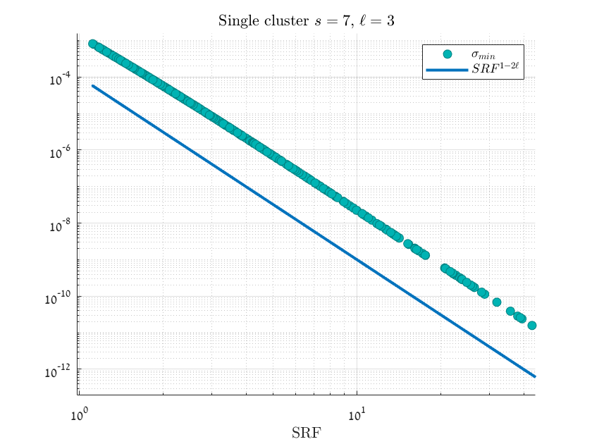
(a) Single Cluster

(b) Multi Cluster, $\ell=\ell_{max}$

Figure 1: Decay rate of $\sigma_{\min}$ as a function of $SRF$. Results of $n=1000$ random experiments with randomly chosen $\Delta,N$ are plotted versus the theoretical bound ${SRF}^{1-2\ell}$.

We also show in figure 2 that the vector $u$ defined in ($\star$ ‣ 4.4) is indeed an approximate minimal singular vector, by plotting the Rayleigh quotient $\frac{\|\Phi_{M}(\boldsymbol{\omega})u\|_{2}}{\|u\|_{2}}$ versus the minimal singular value $\sigma_{\min}(\Phi_{M}(\boldsymbol{\omega}))$, where $\Phi_{M}$ is the confluent Vandermonde matrix as in Definition 4.3 and $\boldsymbol{\omega}$ is a single-cluster equispaced configuration.

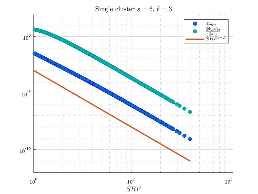
Figure 2: The Rayleigh quotient of the vector $u$ defined in ($\star$ ‣ 4.4) versus the minimal singular value of $\Phi_{M}$. We can see that they scale the same and differ by a constant.

Finally, in order to validate the bounds of Theorem 3.3, we computed the $\ell^{2}$ min-max error $\mathcal{E}$ as in Definition 2.10 and also the $\ell^{2}$ errors of estimating the nodes $\mathcal{E}_{\xi}$, and the coefficients $\mathcal{E}_{a}$, $\mathcal{E}_{b}$ of the worst-case discrete distribution $\mu$ defined by (8) assuming $s=\ell$. We used the ESPRIT (Estimation of Signal Parameters via Rotation Invariance Techniques) [23] method for recovering the nodes $\{t_{j}\}_{j=1}^{s}$ (see more about this method in appendix B). ESPRIT is considered to be one of the best performing subspace methods for estimating parameters of model (1) with white Gaussian noise. Originally developed in the context of frequency estimation [24], it has been generalized to the full model (5) in [14]. Recently it has been shown that if the noise level $\varepsilon$ in the measurements (2) is sufficiently small, the error committed by ESPRIT for estimating the nodes of the simple model (1) is nearly min-max [25]. Consequently, we conjecture the same near-optimal behaviour in the model (4). In order to recover the coefficients $a_{j}$, $b_{j}$ we solve a linear system of equations by the Least Squares method:

$$\min\|U_{N}(\tilde{\boldsymbol{\xi}})v_{\mu}-y\|_{2}\ ,$$

where $\boldsymbol{\tilde{\xi}}$ are the recovered nodes. Note that we prove the theoretical bound to the on-grid model however the ESPRIT algorithm recovers the nodes without taking the grid assumption into account. We have checked two cases:

1. Figure 3(a) - A single equispaced cluster of size $s=\ell=2$ with error $\varepsilon=10^{-12}$.

2. Figure 4(a) - A single equispaced cluster of size $s=\ell=3$ with error $\varepsilon=10^{-12}$.

Our results suggest that the ESPRIT method might indeed be optimal, meaning that it attains the min-max error bounds we established in Theorem 3.3 for the recovered parameters of signal (4).

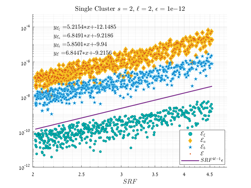
(a)

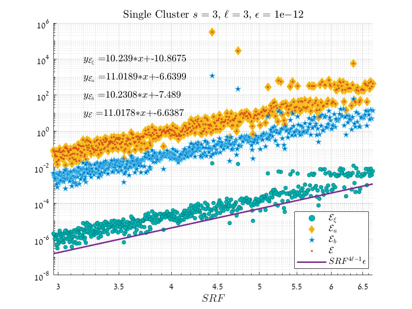
(a)

Figure 4: Accuracy of ESPRIT. Results of n=500 random experiments with randomly chosen $\Delta$ and fixed $N$ are plotted versus the theoretical bound ${SRF}^{4\ell-1}\varepsilon$.

Note that all figures are in logarithmic scale.

The code for the above experiments is available at https://github.com/Gnflu/SR-of-conVan-sys.git

Appendix A Computations for Theorem 3.2

A.1 Finite difference coefficients

We seek approximation of the form:

$$D_{M}^{(2\ell-1)}(\omega)\approx\sum_{i=1}^{\ell}A_{i}D_{M}(x_{i})+B_{i}D^{\prime}_{M}(x_{i})=S_{A,B}(\omega)$$

where

$$x_{i}=\omega-\tau_{i}\Delta,\quad\Delta=\frac{\alpha}{M}\ ,$$

and

$$S_{A,B}(\omega)=\sum_{i=1}^{\ell}A_{i}D_{M}(x_{i})+B_{i}D^{\prime}_{M}(x_{i})=\sum_{i=1}^{\ell}A_{i}D_{M}(\omega+x_{i}-\omega)+B_{i}D^{\prime}_{M}(\omega+x_{i}-\omega).$$

Let $h_{i}:=x_{i}-\omega=-\tau_{i}\Delta=\tau_{i}h$, $h=-\Delta$. Then by Taylor expansion of $D_{M}(\omega+h_{i})$ and using the integral form of the remainder we have:

$$S_{A,B}(\omega)=\sum_{i=1}^{\ell}A_{i}\bigg{(}\sum_{k=0}^{2\ell-1}\frac{D^{(k)}_{M}(\omega)}{k!}h_{i}^{k}+\int_{\omega}^{\omega+h_{i}}\frac{D_{M}^{(2\ell)}(t)}{(2\ell-1)!}(\omega+h_{i}-t)^{2\ell-1}\,dt\bigg{)}$$

$$+B_{i}\bigg{(}\sum_{k=0}^{2\ell-2}\frac{D^{(k+1)}_{M}(\omega)}{k!}h_{i}^{k}+\int_{\omega}^{\omega+h_{i}}\frac{D_{M}^{(2\ell)}(t)}{(2\ell-2)!}(\omega+h_{i}-t)^{2\ell-2}\,dt\bigg{)}$$

By the change of variable $t=\omega+h_{i}r$ we have $dt=h_{i}dr$ and therefore

$$S_{A,B}(\omega) =\sum_{k=0}^{2\ell-1}\frac{D_{M}^{(k)}(\omega)}{k!}\big{(}\sum_{i=1}^{\ell}A_{i}h_{i}^{k}\big{)}+\sum_{k=0}^{2\ell-2}\frac{D_{M}^{(k+1)}(\omega)}{k!}\big{(}\sum_{i=1}^{\ell}B_{i}h_{i}^{k}\big{)}$$

$$\qquad+\frac{1}{(2\ell-1)!}\sum_{i=1}^{\ell}A_{i}\int_{0}^{1}D_{M}^{(2\ell)}(\omega+h_{i}r)(h_{i}-h_{i}r)^{2\ell-1}h_{i}\,dr$$

$$\qquad+\frac{1}{(2\ell-2)!}\sum_{i=1}^{\ell}B_{i}\int_{0}^{1}D_{M}^{(2\ell)}(\omega+h_{i}r)(h_{i}-h_{i}r)^{2\ell-2}h_{i}\,dr$$

$$=P(\omega)+R_{A}(\omega)+R_{B}(\omega),$$

where

$$P(\omega) =\sum_{k=0}^{2\ell-1}\frac{D_{M}^{(k)}(\omega)}{k!}\big{(}\sum_{i=1}^{\ell}A_{i}h_{i}^{k}\big{)}+\sum_{k=0}^{2\ell-2}\frac{D_{M}^{(k+1)}(\omega)}{k!}\big{(}\sum_{i=1}^{\ell}B_{i}h_{i}^{k}\big{)}\ ,$$

$$R_{A}(\omega) =\frac{1}{(2\ell-1)!}\sum_{i=1}^{\ell}A_{i}\int_{0}^{1}D_{M}^{(2\ell)}(\omega+h_{i}r)(h_{i}-h_{i}r)^{2\ell-1}h_{i}\,dr\ ,$$

$$R_{B}(\omega) =\frac{1}{(2\ell-2)!}\sum_{i=1}^{\ell}B_{i}\int_{0}^{1}D_{M}^{(2\ell)}(\omega+h_{i}r)(h_{i}-h_{i}r)^{2\ell-2}h_{i}\,dr.$$

We seek $A_{1},\dots,A_{\ell}$ and $B_{1},\dots,B_{\ell}$ so that $P(\omega)\equiv D_{M}^{(2\ell-1)}(\omega)$, thus the following equations should be fulfilled:

1. $$\sum_{i=1}^{\ell}A_{i}=0$$

2. $$\sum_{i=1}^{\ell}(A_{i}+\frac{kB_{i}}{h_{i}})h_{i}^{k}=0\quad\quad k=1,\dots,2\ell-2$$

3. $$\sum_{i=1}^{\ell}(A_{i}+\frac{(2\ell-1)B_{i}}{h_{i}})h_{i}^{2\ell-1}=(2\ell-1)!$$

This is equivalent to solving the following linear system of equations:

$$U_{2\ell}\begin{pmatrix}A_{1}\\ \vdots\\ A_{\ell}\\ B_{1}\\ \vdots\\ B_{\ell}\\ \end{pmatrix}=\begin{pmatrix}0\\ \vdots\\ \vdots\\ 0\\ (2\ell-1)!\\ \end{pmatrix}\ ,$$

where

$$U_{2\ell}=\begin{pmatrix}1&\dots&1&0&\dots&0\\ h_{1}&\dots&h_{\ell}&1&\dots&1\\ \vdots&\dots&\vdots&\vdots&\dots&\vdots\\ h_{1}^{2\ell-1}&\dots&h_{\ell}^{2\ell-1}&(2\ell-1)h_{1}^{2\ell-2}&\dots&(2\ell-1)h_{\ell}^{2\ell-2}\end{pmatrix}\ .$$

Thus $A_{j},B_{j}$ are given by:

$$\begin{pmatrix}A_{1}\\ \vdots\\ A_{\ell}\\ B_{1}\\ \vdots\\ B_{\ell}\end{pmatrix}=U^{-1}_{2\ell}\begin{pmatrix}0\\ \vdots\\ \vdots\\ 0\\ (2\ell-1)!\end{pmatrix}. \star\star$$ ()

In particular, if $U^{-1}_{2\ell}=\begin{pmatrix}V\\ W\end{pmatrix}$ then $A_{j}=(2\ell-1)!v_{j,2\ell}$ and $B_{j}=(2\ell-1)!w_{j,2\ell}$, where $V,W\in\mathbb{C}^{\ell\times 2\ell}$ and $v_{i,j},\ w_{i,j}$ denote the $(i,j)th$ entry of $V,W$ respectively.

A.2 Proof of Lemma 4.5

Let

$$h_{*}:=\operatorname*{arg\,max}_{h_{i}}\bigg{|}\int_{0}^{1}D_{M}^{(2\ell)}(\omega+h_{i}r)(h_{i}-h_{i}r)^{2\ell-1}h_{i}\,dr\bigg{|}$$

Using the Cauchy-Schwartz inequality we have

$$\big{\|}R_{A}(\omega)\big{\|}^{2}_{L^{2}(\mathbb{T})} =\frac{1}{(2\ell-1)!^{2}}\bigg{\|}\sum_{i=1}^{\ell}A_{i}\int_{0}^{1}D_{M}^{(2\ell)}(\omega+h_{i}r)(h_{i}-h_{i}r)^{2\ell-1}h_{i}\,dr\bigg{\|}^{2}_{L^{2}(\mathbb{T})}$$

$$=\frac{1}{(2\ell-1)!^{2}}\int_{0}^{1}\bigg{|}\sum_{i=1}^{\ell}A_{i}\int_{0}^{1}D_{M}^{(2\ell)}(\omega+h_{i}r)(h_{i}-h_{i}r)^{2\ell-1}h_{i}\,dr\bigg{|}^{2}\,d\omega$$

$$\leq\frac{1}{(2\ell-1)!^{2}}\bigg{(}\sum_{i=1}^{\ell}\big{|}A_{i}\big{|}\bigg{)}^{2}\int_{0}^{1}\bigg{|}\int_{0}^{1}D_{M}^{(2\ell)}(\omega+h_{*}r)(h_{*}-h_{*}r)^{2\ell-1}h_{*}\,dr\bigg{|}^{2}\,d\omega$$

$$\leq\frac{1}{(2\ell-1)!^{2}}\bigg{(}\sum_{i=1}^{\ell}\big{|}A_{i}\big{|}\bigg{)}^{2}\int_{0}^{1}\bigg{(}\int_{0}^{1}\big{|}D_{M}^{(2\ell)}(\omega+h_{*}r)\big{|}^{2}\,dr\int_{0}^{1}\big{|}h_{*}-h_{*}r\big{|}^{4\ell-2}h_{*}^{2}\,dr\bigg{)}\,d\omega$$

$$\leq\frac{1}{(2\ell-1)!^{2}}\bigg{(}\sum_{i=1}^{\ell}\big{|}A_{i}\big{|}\bigg{)}^{2}\int_{0}^{1}\bigg{(}\int_{0}^{1}|D_{M}^{(2\ell)}(\omega+h_{*}r)|^{2}\,dr|\tau\Delta|^{4\ell}\bigg{)}\,d\omega$$

$$\leq\frac{1}{(2\ell-1)!^{2}}\bigg{(}\sum_{i=1}^{\ell}\big{|}A_{i}\big{|}\bigg{)}^{2}\big{|}\tau\Delta\big{|}^{4\ell}\int_{0}^{1}\bigg{(}\int_{0}^{1}|D_{M}^{(2\ell)}(\omega+h_{*}r)|^{2}\,d\omega\bigg{)}\,dr$$

$$\leq\frac{1}{(2\ell-1)!^{2}}\bigg{(}\sum_{i=1}^{\ell}\big{|}A_{i}\big{|}\bigg{)}^{2}\big{|}\tau\Delta\big{|}^{4\ell}\big{\|}D_{M}^{(2\ell)}\big{\|}^{2}_{L^{2}(\mathbb{T})}$$

$$\leq\frac{\tau^{4\ell}}{(2\ell-1)!^{2}}\bigg{(}\sum_{i=1}^{\ell}\big{|}A_{i}\big{|}\bigg{)}^{2}\Delta^{4\ell}(M+1)(2\pi M)^{4\ell}$$

Similarly we get that:

$$\|R_{B}(\omega)\|^{2}_{L^{2}(\mathbb{T})}\leq\frac{\tau^{4\ell-2}}{(2\ell-1)!^{2}}\bigg{(}\sum_{i=1}^{\ell}\big{|}B_{i}\big{|}\bigg{)}^{2}\Delta^{4\ell-2}(M+1)(2\pi M)^{4\ell}$$

A.3 Proof of Lemma 4.6

Recall the definitions of $v_{i,j}$ and $w_{i,j}$ from Appendix A.1. From expressions (3.10) and (3.12) evaluated in Gautchi’s paper [26], and using that $M\leq\frac{1}{\Delta}$ we have:

1. On one hand

   $$\sum_{\mu=1}^{2\ell}\big{|}v_{n,\mu}\big{|} \leq\Bigg{(}\bigg{|}1+2h_{n}\sum_{\nu\neq n}\frac{1}{(h_{n}-h_{\nu})}\bigg{|}+2\bigg{|}\sum_{\nu\neq n}\frac{1}{(h_{n}-h_{\nu})}\bigg{|}\Bigg{)}\prod_{\nu\neq n}\Big{(}\frac{1+|h_{\nu}|}{|h_{n}-h_{\nu}|}\Big{)}^{2}$$

   $$\leq\Bigg{(}\bigg{|}1+2\tau_{n}h\sum_{\nu\neq n}\frac{1}{(\tau_{n}-\tau_{\nu})h}\bigg{|}+2\bigg{|}\sum_{\nu\neq n}\frac{1}{(\tau_{n}-\tau_{\nu})h}\bigg{|}\Bigg{)}\prod_{\nu\neq n}\Big{(}\frac{1+|\tau_{\nu}h|}{|(\tau_{n}-\tau_{\nu})h|}\Big{)}^{2}$$

   $$\leq\Big{(}\big{|}1+2{\tau(\ell-1)}\big{|}+\big{|}\frac{2\ell}{h}\big{|}\Big{)}\Big{(}\frac{1+\tau|h|}{|h|}\Big{)}^{2\ell-2}$$

   $$=\Big{(}1+2\tau\ell-2\tau+2\ell\frac{M}{\alpha}\Big{)}\Big{(}\frac{M}{\alpha}+\tau\Big{)}^{2\ell-2}$$

   $$\leq 2\ell\Big{(}\frac{M}{\alpha}+\tau\Big{)}^{2\ell-1}$$

   $$\leq C_{v}(\ell,\tau)\Big{(}\frac{M}{\alpha}\Big{)}^{2\ell-1}$$

2. On the other hand,

   $$\sum_{\mu=1}^{2\ell}\big{|}w_{n,\mu}\big{|} \leq\big{(}1+|h_{n}|\big{)}\prod_{\nu\neq n}\Big{(}\frac{1+|h_{\nu}|}{|h_{n}-h_{\nu}|}\Big{)}^{2}\leq\big{(}1+\tau|h|\big{)}\Big{(}\frac{1+\tau|h|}{|h|}\Big{)}^{2\ell-2}$$

   $$=\Big{(}1+\tau\frac{\alpha}{M}\Big{)}\Big{(}\frac{M}{\alpha}+\tau\Big{)}^{2\ell-2}\leq 2\Big{(}\frac{M}{\alpha}+\tau\Big{)}^{2\ell-2}$$

   $$\leq C_{w}(\ell,\tau)\Big{(}\frac{M}{\alpha}\Big{)}^{2\ell-2}$$

Now we can evaluate the following expressions:

1. $$\sum_{i=0}^{\ell}|A_{i}| =(2\ell-1)!\sum_{i=1}^{\ell}|v_{i,2\ell}|\leq(2\ell-1)!\sum_{i=1}^{\ell}\sum_{\mu=1}^{2\ell}|v_{i,\mu}|$$

   $$\leq\ell(2\ell-1)!C_{v}(\ell,\tau)\bigg{(}\frac{M}{\alpha}\bigg{)}^{2\ell-1}$$

   $$=C_{A}(\ell,\tau)\bigg{(}\frac{M}{\alpha}\bigg{)}^{2\ell-1}$$

2. $$\sum_{i=0}^{\ell}|B_{i}| =(2\ell-1)!\sum_{i=1}^{\ell}|w_{i,2\ell}|\leq(2\ell-1)!\sum_{i=1}^{\ell}\sum_{\mu=1}^{2\ell}|w_{i,\mu}|$$

   $$\leq\ell(2\ell-1)!C_{w}(\ell,\tau)\bigg{(}\frac{M}{\alpha}\bigg{)}^{2\ell-2}$$

   $$=C_{B}(\ell,\tau)\bigg{(}\frac{M}{\alpha}\bigg{)}^{2\ell-2}$$

A.4 Proof of Lemma 4.4

For any tempered distribution $\mu$ supported in $\mathbb{T}$, we will show that the following is true:

$$\sum_{m=0}^{M}\big{|}\hat{\mu}(m)\big{|}^{2}=\big{\|}\mu*D_{M}\big{\|}^{2}_{L^{2}(\mathbb{T})}$$

First:

$$(\mu*D_{M})(\omega) =\int_{0}^{1}\mu(y)D_{m}(\omega-y)\,dy=\int_{0}^{1}\mu(y)\sum_{m=0}^{M}e^{2\pi im(\omega-y)}\,dy$$

$$=\sum_{m=0}^{M}e^{2\pi im\omega}\bigg{(}\int_{0}^{1}\mu(y)e^{-2\pi imy}\,dy\bigg{)}$$

$$=\sum_{m=0}^{M}\hat{\mu}(m)e^{2\pi im\omega}\ .$$

Now we can show the desired equality:

$$\big{\|}(\mu*D_{M})(\omega)\big{\|}^{2}_{L^{2}(\mathbb{T})} =\int_{0}^{1}\big{|}\sum_{m=0}^{M}e^{2\pi im\omega}\hat{\mu}(m)\big{|}^{2}\,d\omega=\int_{0}^{1}\big{(}\sum_{m=0}^{M}e^{2\pi im\omega}\hat{\mu}(m)\big{)}\overline{\big{(}\sum_{m=0}^{M}e^{2\pi im\omega}\hat{\mu}(m)\big{)}}\,d\omega$$

$$=\int_{0}^{1}\sum_{m=0}^{M}\big{|}e^{2\pi im\omega}\hat{\mu}(m)\big{|}^{2}+\sum_{m=0}^{M}\sum_{k\neq m}e^{2\pi i(m-k)\omega}\hat{\mu}(m)\overline{\hat{\mu}(k)}\,d\omega$$

$$=\sum_{m=0}^{M}\big{|}\hat{\mu}(m)\big{|}^{2}+\sum_{m=0}^{M}\sum_{k\neq m}\hat{\mu}(m)\overline{\hat{\mu}(k)}\int_{0}^{1}e^{2\pi i(m-k)\omega}\,d\omega$$

$$=\sum_{m=0}^{M}\big{|}\hat{\mu}(m)\big{|}^{2}\qed$$

A.5 Proof of Lemma 4.7

Let $U_{2\ell}$ be defined as in (A.1), and let

$$X=\begin{pmatrix}A_{1}\\ \vdots\\ A_{\ell}\\ B_{1}\\ \vdots\\ B_{\ell}\end{pmatrix},\quad b=\begin{pmatrix}0\\ \vdots\\ \vdots\\ 0\\ (2\ell-1)!\end{pmatrix}$$

As in appendix A.1 we know that:

$$U_{2\ell}x=b$$

We can write (*) as:

$$\underbrace{\begin{pmatrix}1&&&\\ &h&&\\ &&\ddots&\\ &&&h^{2\ell-1}\end{pmatrix}}_{D}\underbrace{\begin{pmatrix}1&\dots&1&0&\dots&0\\ \tau_{1}&\dots&\tau_{\ell}&1&\dots&1\\ \vdots&\dots&\vdots&\vdots&\dots&\vdots\\ \tau_{1}^{2\ell-1}&\dots&\tau_{\ell}^{2\ell-1}&(2\ell-1)\tau_{1}^{2\ell-2}&\dots&(2\ell-1)\tau_{\ell}^{2\ell-2}\end{pmatrix}}_{L}\underbrace{\begin{pmatrix}A_{1}\\ \vdots\\ A_{\ell}\\ \frac{B_{1}}{h}\\ \vdots\\ \frac{B_{\ell}}{h}\end{pmatrix}}_{y}=b$$

$$y=L^{-1}D^{-1}b,\quad x=\operatorname{diag}(1,\dots,1,h,\dots,h)y$$

$$x=\begin{pmatrix}I&0\\ 0&hI\end{pmatrix}L^{-1}D^{-1}b=\begin{pmatrix}I&0\\ 0&hI\end{pmatrix}L^{-1}\begin{pmatrix}0\\ \vdots\\ 0\\ (2\ell-1)!h^{1-2\ell}\end{pmatrix}=\begin{pmatrix}{(L^{-1})}_{1,2\ell}(2\ell-1)!h^{1-2\ell}\\ \vdots\\ {(L^{-1})}_{\ell,2\ell}(2\ell-1)!h^{1-2\ell}\\ {(L^{-1})}_{\ell+1,2\ell}(2\ell-1)!h^{2-2\ell}\\ \vdots\\ {(L^{-1})}_{2\ell,2\ell}(2\ell-1)!h^{2-2\ell}\end{pmatrix}$$

$$\|x\|^{2}_{2}=\sum_{i=1}^{\ell}{(L^{-1})}_{i,2\ell}^{2}{(2\ell-1)!}^{2}h^{2(1-2\ell)}+\sum_{i=1}^{\ell}{(L^{-1})}_{\ell+i,2\ell}^{2}{(2\ell-1)!}^{2}h^{2(2-2\ell)}\geq\sum_{i=1}^{2\ell}{(L^{-1})}_{i,2\ell}^{2}{(2\ell-1)!}^{2}\Delta^{2-4\ell}$$

$$\sum_{i=1}^{2\ell}{(L^{-1})}_{i,2\ell}^{2}=\|L^{-1}(0,...,0,1)^{T}\|_{2}^{2}\geq\min_{\|w\|_{2}=1}\|L^{-1}w\|_{2}^{2}=\sigma_{\min}^{2}(L^{-1})=\frac{1}{\sigma_{max}^{2}(L)}=\frac{1}{\|L\|_{2}^{2}}\geq\frac{1}{rank(L)\|L\|_{\infty}^{2}}$$

$$\|L\|_{\infty}\leq\sum_{i=1}^{\ell}\tau_{i}^{2\ell-1}+\sum_{i=1}^{\ell}(2\ell-1)\tau_{i}^{2\ell-2}\leq\ell(\tau^{2\ell-1}+(2\ell-1)\tau^{2\ell-2})\leq 2\ell^{2}\tau^{2\ell-1}$$

$$\|x\|_{2}^{2}\geq\frac{{(2\ell-1)!}^{2}\Delta^{2-4\ell}}{2\ell{(2\ell^{2}\tau^{2\ell-1})}^{2}}\Rightarrow\|x\|_{2}\geq\frac{(2\ell-1)!\Delta^{1-2\ell}}{\sqrt{8\ell^{5}}\tau^{2\ell-1}}=C_{3}(\ell,\tau)\Delta^{1-2\ell}$$

Finally, for $u$ defined in ($\star$ ‣ 4.4), we have

$$u=\Delta^{2\ell-1}\begin{pmatrix}I&0\\ 0&\mathbf{Z}\end{pmatrix}X=\Delta^{2\ell-1}\mathbf{Z}x,\quad\mathbf{Z}=\operatorname{diag}(z_{1},\dots,z_{\ell})$$

$$\|u\|_{2} =\Delta^{2\ell-1}\|\mathbf{Z}x\|_{2}\|\mathbf{Z}^{-1}\|_{2}\|\mathbf{Z}^{-1}\|^{-1}_{2}$$

$$\geq\Delta^{2\ell-1}\|\mathbf{Z}\mathbf{Z}^{-1}x\|_{2}\|\mathbf{Z}^{-1}\|^{-1}_{2}=\Delta^{2\ell-1}\|x\|_{2}\|\mathbf{Z}^{-1}\|^{-1}_{2}$$

$$\geq\frac{1}{\sqrt{2\ell}}\Delta^{2\ell-1}\Delta^{1-2\ell}C_{3}(\ell,\tau)=\tilde{C}_{3}(\ell,\tau)$$

We used in last inequality the following property:

$$\|\mathbf{Z}\|_{2}\leq\sqrt{rank(\mathbf{Z})}\|\mathbf{Z}\|_{\infty}$$

Appendix B ESPRIT Method

We provide the description of the matrix for completeness, see e.g. [14, 12].

Definition B.1 (Hankel Matrix).

Let $\mu(x)=\sum_{j=1}^{s}a_{j}\delta(x-t_{j})+b_{j}\delta^{\prime}(x-t_{j})$, $a_{j},b_{j}\in\mathbb{C}$ and $\boldsymbol{t}=(t_{1},\dots,t_{s})$, $t_{j}\in\mathbb{T}$, thus

$$m_{k}:=\hat{\mu}(k)=\sum_{j=1}^{s}a_{j}e^{-2\pi ikt_{j}}+2\pi ikb_{j}e^{-2\pi ikt_{j}}=\sum_{j=1}^{s}a_{j}z_{j}^{k}+2\pi ikb_{j}z_{j}^{k}$$

Then we define the $C\times C$ Hankel matrix as follows:

$$H_{C}:=\begin{pmatrix}m_{0}&m_{1}&\dots&m_{C-1}\\ m_{1}&m_{2}&\dots&m_{C}\\ \vdots&\vdots&\vdots&\vdots\\ m_{C-1}&m_{C}&\dots&m_{2C-2}\end{pmatrix}$$

where $C:=2s$ (number of unknown coeffients).

The ESPRIT (and other subspace methods) relies on the following observations:

1. The range (column space) of both the data matrix $H_{C}$ (B.1) and the confluent Vandermonde matrix $\Phi:=\Phi_{2C-1}$ 2.1 are the same, namely $H_{C}$ admits the following factorization:

   $$H_{C}=\Phi B\Phi^{T}\ ,$$

   where $B:=\operatorname{diag}(a_{1},\dots,a_{s},b_{1},\dots,b_{s})$.

2. The matrix $\Phi$ has the so-called rotational invariance property [14]:

   $$\Phi^{\uparrow}=\Phi^{\downarrow}J$$

   where $\Phi^{\uparrow}$ denotes $\Phi$ without the first row, $\Phi^{\downarrow}$ denotes $\Phi$ without the last row, and $J$ is a block diagonal matrix whose $i^{\text{th}}$ block is the $2\times 2$ Jordan block with the node $z_{i}$ on the diagonal.

Suppose we know $\Phi$; then the matrix $J$ could be found by

$$J=\Phi_{\downarrow}^{\#}\Phi^{\uparrow}$$

(where $\#$ denotes the Moore–Penrose pseudoinverse), and then the nodes $z_{j}$ could be recovered as the eigenvalues of $J$.

Unfortunately, $\Phi$ is unknown in advance, but suppose we had at our disposal a matrix $W$ whose column space was identical to that of $\Phi$. In that case, we would have $W=\Phi G$ for an invertible $G$, and consequently

$$W^{\uparrow}=W^{\downarrow}\Psi,$$

where

$$\Psi=G^{-1}JG,$$

which means that the eigenvalues of $\Psi$ are also $\{z_{j}\}$. Such a matrix $W$ can be obtained, for example, from the singular value decomposition (SVD) of the data matrix/covariance matrix. To summarize, the ESPRIT method for estimating $\{z_{j}\}$, as used in our experiments below, is as follows.

1:A $C\times C$ Hankel matrix $H_{C}$ built from the measurements.

2:Recovered nodes $\{z_{j}\}$.

3:Compute the SVD $H_{C}=W\Sigma V^{T}$

4:Calculate $\Psi=W^{\#}_{\downarrow}W^{\uparrow}$

5:Set $\{z_{j}\}$ to be the eigenvalues of $\Psi$ with appropriate multiplicities (use, e.g., arithmetic neans to estimate multiple nodes which are scattered by the noise).

Algorithm 1 ESPRIT method for recovering the nodes $\{z_{j}\}$

References

• [1] D.L. Donoho “Superresolution via Sparsity Constraints” In SIAM Journal on Mathematical Analysis 23.5, 1992, pp. 1309–1331
• [2] Dmitry Batenkov, Benedikt Diederichs, Gil Goldman and Yosef Yomdin “The Spectral Properties of Vandermonde Matrices with Clustered Nodes” In Linear Algebra and its Applications 609, 2021, pp. 37–72 DOI: 10.1016/j.laa.2020.08.034
• [3] Dmitry Batenkov, Gil Goldman and Yosef Yomdin “Super-Resolution of near-Colliding Point Sources” In Information and Inference: A Journal of the IMA 10.2 Oxford Academic, 2021, pp. 515–572 DOI: 10.1093/imaiai/iaaa005
• [4] Dmitry Batenkov, Laurent Demanet, Gil Goldman and Yosef Yomdin “Conditioning of Partial Nonuniform Fourier Matrices with Clustered Nodes” In SIAM Journal on Matrix Analysis and Applications 44.1, 2020, pp. 199–220 DOI: 10/ggjwzb
• [5] Weilin Li and Wenjing Liao “Stable super-resolution limit and smallest singular value of restricted Fourier matrices” In Applied and Computational Harmonic Analysis 51, 2020, pp. 118–156 DOI: 10.1016/j.acha.2020.10.004
• [6] Emmanuel J. Candès and Carlos Fernandez-Granda “Towards a Mathematical Theory of Super-resolution” In Communications on Pure and Applied Mathematics 67.6, 2014, pp. 906–956 DOI: 10.1002/cpa.21455
• [7] Laurent Demanet and Nam Nguyen “The Recoverability Limit for Superresolution via Sparsity” In arXiv preprint arXiv:1502.01385, 2015 arXiv:1502.01385
• [8] Mathias Hockmann and Stefan Kunis “Sparse Super Resolution Is Lipschitz Continuous” In arXiv:2108.11925 [cs, math], 2021 arXiv:2108.11925 [cs, math]
• [9] Ping Liu and Hai Zhang “A Theory of Computational Resolution Limit for Line Spectral Estimation” In IEEE Transactions on Information Theory 67.7, 2021, pp. 4812–4827 DOI: 10.1109/TIT.2021.3075149
• [10] Markus Petz, Gerlind Plonka and Nadiia Derevianko “Exact Reconstruction of Sparse Non-Harmonic Signals from Their Fourier Coefficients” In Sampling Theory, Signal Processing, and Data Analysis 19.1, 2021, pp. 7 DOI: 10.1007/s43670-021-00007-1
• [11] Annie Cuyt and Wen-shin Lee “How to Get High Resolution Results from Sparse and Coarsely Sampled Data” In Applied and Computational Harmonic Analysis, 2018 DOI: 10/ggb5cv
• [12] D. Batenkov and Y. Yomdin “On the Accuracy of Solving Confluent Prony Systems” In SIAM J. Appl. Math. 73.1, 2013, pp. 134–154 DOI: 10.1137/110836584
• [13] Dmitry Batenkov “Stability and Super-Resolution of Generalized Spike Recovery” In Applied and Computational Harmonic Analysis 45.2, 2018, pp. 299–323 DOI: 10.1016/j.acha.2016.09.004
• [14] R Badeau, G Richard and B David “High-resolution spectral analysis of mixtures of complex exponentials modulated by polynomials” In IEEE transactions on signal processing 54.4, 2006, pp. 1341–1350
• [15] D. Batenkov and Y. Yomdin “Algebraic Fourier Reconstruction of Piecewise Smooth Functions” In Mathematics of Computation 81, 2012, pp. 277–318 DOI: 10.1090/S0025-5718-2011-02539-1
• [16] Dmitry Batenkov “Complete Algebraic Reconstruction of Piecewise-Smooth Functions from Fourier Data” In Mathematics of Computation 84.295, 2015, pp. 2329–2350 DOI: 10.1090/S0025-5718-2015-02948-2
• [17] Avram Sidi “Interpolation at equidistant points by a sum of exponential functions” In Journal of approximation theory 34.2, 1982, pp. 194–210 DOI: 10.1016/0021-9045(82)90092-2
• [18] R Badeau, G Richard and B David “Performance of ESPRIT for Estimating Mixtures of Complex Exponentials Modulated by Polynomials” In IEEE transactions on signal processing 56.2, 2008, pp. 492–504
• [19] Dmitry Batenkov and Gil Goldman “Single-exponential bounds for the smallest singular value of Vandermonde matrices in the sub-Rayleigh regime” In Applied and Computational Harmonic Analysis 55, 2021 DOI: 10.1016/j.acha.2021.07.003
• [20] W. Gautschi “On inverses of Vandermonde and confluent Vandermonde matrices” In Numerische Mathematik 4.1, 1962, pp. 117–123 URL: https://doi.org/10.1007/BF01386302
• [21] Roger A. Horn and Charles R. Johnson “Matrix Analysis” New York: Cambridge University Press, 2013
• [22] S.. Bernstein “Sur l’ordre de la meilleure approximation des fonctions continues par les polynômes de degré donn” In Mémoires publiés par la Classe des Sciences de l’Académie de Belgiqu 4, 1912
• [23] Thomas Kailath and Richard H. Roy III “ESPRIT–Estimation of Signal Parameters via Rotational Invariance Techniques” In Optical Engineering 29.4, 1990, pp. 296–313
• [24] Petre Stoica and Randolph Moses “Spectral Analysis of Signals” Upper Saddle River, N.J. : Pearson/Prentice Hall, 2005
• [25] Weilin Li, Wenjing Liao and Albert Fannjiang “Super-Resolution Limit of the ESPRIT Algorithm” In IEEE transactions on information theory 66.7, 2020, pp. 4593–4608
• [26] W. Gautschi “On inverses of Vandermonde and confluent Vandermonde matrices II” In Numerische Mathematik 5, 1963, pp. 425–430