Theoretical description of time-resolved photoemission in charge-density-wave materials out to long times

Abstract

We describe coupled electron-phonon systems semiclassically—Ehrenfest dynamics for the phonons and quantum mechanics for the electrons—using a classical Monte Carlo approach that determines the nonequilibrium response to a large pump field. The semiclassical approach is quite accurate, because the phonons are excited to average energies much higher than the phonon frequency, eliminating the need for a quantum description. The numerical efficiency of this method allows us to perform a self-consistent time evolution out to very long times (tens of picoseconds) enabling us to model pump-probe experiments of a charge density wave (CDW) material. Our system is a half-filled, one-dimensional (1D) Holstein chain that exhibits CDW ordering due to a Peierls transition. The chain is subjected to a time-dependent electromagnetic pump field that excites it out of equilibrium, and then a second probe pulse is applied after a time delay. By evolving the system to long times, we capture the complete process of lattice excitation and subsequent relaxation to a new equilibrium, due to an exchange of energy between the electrons and the lattice, leading to lattice relaxation at finite temperatures. We employ an indirect (impulsive) driving mechanism of the lattice by the pump pulse due to the driving of the electrons by the pump field. We identify two driving regimes, where the pump can either cause small perturbations or completely invert the initial CDW order. Our work successfully describes the ringing of the amplitude mode in CDW systems that has long been seen in experiment, but never successfully explained by microscopic theory.

Time-resolved angle-resolved photoemission spectroscopy (trARPES) is an ultrafast measuring technique Sobota et al. (2021) capable of capturing the real-time evolution and occupation of electronic states in an array of materials: from superconductors, Gerber et al. (2017) semimetals such as graphene Aeschlimann et al. (2021) to topological insulators. Sobota et al. (2012) A particular focus is given to CDW materials Gruner (1994); Grüner (1988) due to the specific ordering nature of their ground state and different competing phases they can exhibit. The trARPES experiments utilize a combination of time-delayed pump and probe pulses to excite the studied material and track the dynamics of the induced nonequilibrium state. The technique was so far successfully used to study oscillations of the CDW amplitude mode, as well as CDW melting in various materials, from $\rm TaS_{2}$ Perfetti et al. (2006, 2008) to rare-earth tritellurides such as $\rm TbTe_{3}$, Schmitt et al. (2008, 2011); Maklar et al. (2021) $\rm LaTe_{3}$, Kogar et al. (2020) and $\rm DyTe_{3}$. Zong et al. (2021)

In a typical trARPES experiment, the pump-induced modification of the electronic structure is observed in the measured photoemission spectrum (PES). The lattice can be driven due to direct dipole coupling with the pump field or indirectly through coupling with electrons. The conventional explanation of the indirect driving involves the transfer of energy from the laser pump to electrons, happening on a femtosecond timescale, and then from electrons to the crystal lattice, happening on a picosecond timescale. A detailed understanding of this driving mechanism is essential in the context of Floquet engineering Hübener et al. (2018) where the dressing of the electronic structure by lattice motion can be used to fine-tune the electronic spectrum.

The theoretical description of pump-probe experiments for CDW systems has relied on phenomenological approaches like time-dependent Ginzburg-Landau theory, whereas the study of microscopic models has been hindered by the absence of efficient numerical methods that can resolve the very different timescales of electron and phonon dynamics. Dynamical mean-field theory Moritz et al. (2010); Matveev et al. (2016) and related studies Shen et al. (2014a, b); Freericks et al. (2017) focused on the excitation of the nonequilibrium electronic state for several tens of femtoseconds, but the slow lattice motion was not considered. Exact diagonalization and the density-matrix renormalization group can provide exact results for small lattice sizes, short times scales, and high phonon frequencies; De Filippis et al. (2012); Matsueda et al. (2012); Hashimoto and Ishihara (2017); Stolpp et al. (2020); Sous et al. (2021) as time proceeds, the growing number of phonon excitations renders simulations impossible, in particular for phonon frequencies in the meV range which are required for an accurate description of most CDW materials. To explain the indirect driving mechanism, as exemplified by the experiment in Ref. Schmitt et al., 2008, it is necessary to develop approaches that naturally include the slow phonon dynamics. One possibility to achieve this is by the so-called exact factorization, Abedi et al. (2010) while another is by the multitrajectory Ehrenfest method. Lively et al. (2021)

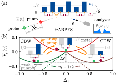
Figure 1: (a) Schematics of the 1D Holstein chain of tight-binding sites (orange dots) with local lattice displacements $\Delta_{i}$ at every site (dark red dots and dark red lines below the orange dots) in our trARPES setup. A pump pulse $E(t)$ excites the electronic charge density $n_{i}$ (dark blue bars) by modifying the Peierls phase factor of the tight-binding hopping parameter $\gamma$. The energy distribution of the injected electrons is captured in the computed photoemission spectrum $P(\omega,t)$. (b) Three potential energy profiles (green parabola, red parabola, and brown parabola) of a single lattice displacement $\Delta_{i}$ (dark red circles and dark red lines on the right side of the three insets above the parabolas) for different values of the onsite charge density $n_{i}$ (blue bars on the right side of the three insets). Green dots show the potential minima of the three parabolas. The system is initialized at $T=0$ temperature. The green and brown parabola with green dots also show the two possible distorted charge density wave states with negative and positive displacements, respectively. For the context of what happens on the neighboring sublattice, see the grayed sites and bars on the left side of the three insets. The two possible distorted states are separated by an energy barrier $\Delta V$. Pump excitation modifies the onsite charge density $n_{i}$, which rotates the potential energy parabola around the $\Delta_{i}=0$ point (see the orange and gray arrows which depict the motion of potential minima for strong and weak pump excitation, respectively). This happens because the derivative of the potential (7) at $\Delta_{i}=0$ is $n_{i}-1/2$ (the dashed green and brown lines). For uniform charge density the system is considered to be metallic (inset above the red parabola) and the derivative is zero.

In this article, we extend a time-dependent Monte Carlo (MC) method, Weber and Freericks (2022) recently developed for frozen phonons, to include the classical lattice motion. This approach is similar to that of ab-initio molecular dynamics, Car and Parrinello (1985) except we focus more on the measurable electronic properties in the context of trARPES experiments. A classical description of the phonons is expected to become accurate if temperature and/or the Peierls gap are larger than the phonon frequency, Brazovskii and Dzyaloshinskii (1976) as confirmed by exact quantum Monte Carlo simulations in equilibrium. Weber et al. (2018) For realistic parameters, this is already the case at very low temperatures. Although the semiclassical approach is poor at zero temperature, because it neglects the quantum fluctuations in the ground state and has no damping, we find that a sliding time average can explain some of the features we observe at finite temperatures. Furthermore, the addition of energy into the system via a strong pump only improves the accuracy of this method, as the quantization of the phonon energies becomes less and less important. For our method to be efficient, we neglect electron-electron interactions; as they mainly affect the short-time decay after the pump, we expect our method to capture the universal long-time features of the induced lattice dynamics. In particular, our method reveals all the details of the indirect driving mechanism found in experiments.

Before explaining the method, we briefly describe our system and summarize our main findings. A simplified schematics of a trARPES setup to which we apply our method is shown in Fig. 1(a). In equilibrium at zero temperature, it is a perfectly-dimerized tight-binding chain in the CDW phase, where alternating lattice displacements $\pm\Delta^{\rm eq}_{i}$ are accompanied by an alternating charge density $n^{\rm eq}_{i}$ varying around 1/2. The indirect driving mechanism can be explained by looking at the potential energy profile of each lattice displacement, as illustrated in Fig. 1(b). The pump perturbs the equilibrium electronic order, thus changing the local charge density $n_{i}(t)$. The perturbed electronic state sets a new potential profile for the phonons at each site by rotating the equilibrium potential parabola around $\Delta_{i}=0$ and setting a new dynamical minimum $\Delta^{\rm min}_{i}(t)$ (green dots in Fig. 1(b)) towards which each local displacement $\Delta_{i}(t)$ tends to move.

The pump can be considered strong or weak depending on its amplitude and frequency. Strong pumps will drive the system from the initial CDW state on the left inset of Fig. 1(b) to an “overshot” state on the right inset with an inverted order parameter. The system left to itself after the pump will oscillate between these two insulating CDW orders by briefly going through a metallic state (the top inset in Fig. 1(b)). Flipping the CDW order, as exemplified by the site considered in Fig. 1(b), means the local charge density $n_{i}(t)$ goes below 1/2 (if initially being above 1/2), while the local displacement $\Delta_{i}(t)$ changes sign. By contrast, weak pumps only slightly perturb the initial CDW. They cause weak oscillations of the local displacements $\Delta_{i}(t)$, but never change their sign. We show both these scenarios, for the weak and the strong pump, in two videos in the Supporting Information Appendix (SI).

The pump-induced lattice motion will change the electronic structure of the system, causing the insulating gap energy to oscillate. The coupled dynamics will repeat until the system reaches a new equilibrium. This behaviour can be deduced from the computed PES (Fig. 2) as well as from the order parameters for the electronic and lattice subsystems (Fig. 3). Additionally, we explore what are the conditions in terms of pump amplitude and frequency which would cause weak or strong driving (Fig. 4). In the pumping regime that we consider, where the photon frequencies are at least one order of magnitude higher than the phonon ones, pump driving is modulated mostly by its amplitude. We find there is a threshold amplitude at which the driving begins, and also another one which determines the transition from the weak to the strong pumping regime. We contrast this with a transient CDW melting regime where the two subsystems are temporarily decoupled and the lattice oscillates at its intrinsic frequency. Additionally, we provide the details of electron dynamics and populations of the two subbands during the pump pulse in the SI.

Overview of the Method

The system illustrated in Fig. 1(a) is modeled by the 1D spinless Holstein model

$$\hat{H}=\hat{H}_{\rm el}+\hat{H}_{\rm ph}\,.$$ (1)

The electronic subsystem consists of a nearest-neighbor tight-binding model with uniform hopping $\gamma$ and an electron-phonon interaction with coupling constant $g$, i.e.,

$$\hat{H}_{\rm el}=-\sum_{i=1}^{L}\left(\gamma\,\hat{c}^{\dagger}_{i}\hat{c}_{i+1}+{\textrm{h.c.}}\right)+\ g\sum_{i=1}^{L}\hat{q}_{i}\left(\hat{n}_{i}-\frac{1}{2}\right).$$ (2)

Here, $\hat{c}^{\dagger}_{i}$ and $\hat{c}_{i}$ are the electronic creation and annihilation operators at lattice site $i$, while $\hat{q}_{i}$ is the local phonon displacement operator coupled to the local charge density $\hat{n}_{i}=\hat{c}^{\dagger}_{i}\hat{c}_{i}$. We impose periodic boundary conditions to eliminate edge effects. A time-varying pump field is implemented via the Peierls substitution $\gamma\to\gamma\,e^{-i\varphi(t)}$ on all sites, thus rendering the electronic Hamiltonian $\hat{H}_{\rm el}(t)$ explicitly time-dependent. Following Refs. Freericks et al., 2009; Shen et al., 2014b, the probe is considered only perturbatively and is not included in the Peierls phase. The second term in the total Hamiltonian consists of the phonon kinetic and potential energy,

$$\hat{H}_{\rm ph}=\sum_{i=1}^{L}\frac{\hat{p}_{i}^{2}}{2M}+\sum_{i=1}^{L}\frac{K}{2}\hat{q}_{i}^{2}\,,$$ (3)

with $K$ being the phonon spring constant and $M$ the phonon mass; $\hat{p}_{i}$ is the phonon momentum operator. We also define the phonon frequency $\Omega=\sqrt{K/M}$ and the dimensionless electron-phonon coupling constant $\lambda=g^{2}/(4K\gamma)$. Through the rest of our paper we use $\gamma$ as the unit of energy and set $\Omega=0.01\,\gamma/\hbar$, $\lambda=0.6$, and $L=30$ if not stated otherwise.

To solve for the long-time dynamics of the coupled electron-phonon system, we treat the electrons quantum mechanically but approximate the phonons by classical variables $q_{i}$ and $p_{i}$. A classical description of the phonons becomes exact in the frozen phonon limit where $M\to\infty$ (i.e., $\Omega\to 0$); furthermore, we describe why the classical description should also be quite accurate when the average energy in the phonons is larger than $\hbar\Omega$ in the SI. While the short-time response of the electrons to an applied pump field can be calculated efficiently in the static limit, the slow energy exchange between electrons and phonons requires small but finite phonon frequencies. To this end, we apply the Ehrenfest theorem to obtain the classical phonon equations of motion

$$\frac{d}{dt}{\Delta}_{i}(t) = \Omega^{2}\pi_{i}(t)\,,$$ (4)

$$\frac{d}{dt}\pi_{i}(t) = -{\Delta}_{i}(t)-4\lambda\gamma\left(n_{i}(t)-1/2\right)\,,$$ (5)

for the rescaled classical variables $\Delta_{i}(t)=g\,q_{i}(t)$ and $\pi_{i}(t)=g\,p_{i}(t)/K$. Here, $n_{i}(t)=\mathopen{\hbox{\set@color${\langle}$}\mkern 2.0mu\kern-3.49998pt\leavevmode\hbox{\set@color${\langle}$}}\hat{n}_{i}(t)\mathclose{\hbox{\set@color${\rangle}$}\mkern 2.0mu\kern-3.49998pt\leavevmode\hbox{\set@color${\rangle}$}}_{\vec{\Delta}_{0},\vec{\pi}_{0}}$ is the electronic expectation value of the charge density at time $t$, considering that the phonons were initialized in a configuration $(\vec{\Delta}_{0},\vec{\pi}_{0})$. The r.h.s. of Eq. (5) defines a force that depends on the local phonon displacement $\Delta_{i}(t)$ and on the charge density $n_{i}(t)$.

For classical phonons, we calculate time-dependent observables $\langle\hat{O}(t)\rangle=\int d\vec{\Delta}_{0}\int d\vec{\pi}_{0}\,W_{\mathrm{eq}}(\vec{\Delta}_{0},\vec{\pi}_{0})\,\mathopen{\hbox{\set@color${\langle}$}\mkern 2.0mu\kern-3.49998pt\leavevmode\hbox{\set@color${\langle}$}}\hat{O}(t)\mathclose{\hbox{\set@color${\rangle}$}\mkern 2.0mu\kern-3.49998pt\leavevmode\hbox{\set@color${\rangle}$}}_{\vec{\Delta}_{0},\vec{\pi}_{0}}$ as a weighted average with respect to the equilibrium phonon distribution $W_{\mathrm{eq}}$. We initialize our system in the equilibrium solution of the static phonon limit, which is accurate for temperatures $k_{\mathrm{B}}T\gtrsim\hbar\Omega$. Weber et al. (2018) Then, the initial phonon displacements $\vec{\Delta}_{0}$ are sampled from $W_{\mathrm{eq}}[\Omega=0]$ using a classical MC method Weber et al. (2016) and we set $\vec{\pi}_{0}=0$. At $T=0$, our system is set up by a single configuration $\Delta_{0,i}=(-1)^{i}\Delta$ with perfect dimerization which is accompanied by CDW order, as illustrated in Fig. 1(a). A band gap of $2\Delta$ separates the fully-filled lower band from the empty upper band, so that the rescaled displacements are directly related to the single-particle gap $\Delta$. Although there is no true long-range CDW order in 1D at $T>0$, the band gap as well as short-range CDW correlations remain stable up to $k_{\mathrm{B}}T\approx 0.1\,\gamma$. For details on the equilibrium solution, see Ref. Weber et al., 2016.

For each initial phonon configuration, the coupled electron-phonon dynamics is implemented self-consistently in two steps. In the first step, we update the electron annihilation operators $\hat{c}_{i}(t+\Delta t)=\sum_{j=1}^{L}\mathcal{U}_{ij}(t+\Delta t,t)\hat{c}_{j}(t)$ through evolution by direct diagonalization (for technical details see Ref. Weber and Freericks, 2022). This allows us to update $n_{i}(t)$. In the second step, the obtained $n_{i}(t)$ is replaced in Eq. (5) and new lattice displacements are computed using the Verlet integration scheme. Because $\hat{H}_{\mathrm{el}}(t)$ is quadratic for each phonon configuration, we only need $\mathcal{O}(L^{3})$ operations for every time step. This allows us to reach long enough times to observe the damped phonon oscillations also found in experiments. Note that the MC average over many initial phonon configurations recovers the interacting nature of our electron-phonon coupled system.

The chain is driven out of equilibrium with an external electric field applied uniformly in space along the $x$ direction,

$$\mathbf{E}(\mathbf{r},t)=E_{0}\exp{\left(-\frac{t^{2}}{2\sigma_{\rm p}^{2}}\right)}\sin{\left(\omega_{\rm p}t\right)}\,\mathbf{e}_{\rm x}\,.$$ (6)

Here, $E_{0}$ is the pump amplitude, $\sigma_{\rm p}$ the pump width, $\omega_{\rm p}$ the pump frequency, and $\mathbf{e}_{\rm x}$ the unit vector along the chain.

Results

Insight on how the lattice is set in motion can be obtained from an effective phonon potential. By integrating the force in Eq. (5), we obtain a potential for a single lattice displacement,

$$V_{i}(\Delta_{i})=\frac{1}{8\lambda\gamma}\Delta_{i}^{2}+\Delta_{i}(n_{i}(t)-1/2)\,,$$ (7)

which is just the sum of the local phonon potential energy and the electron-phonon energy. For the perfectly-dimerized chain, there are two possible ground states which differ from each other by the sign of $\Delta_{i}$ and $n_{i}-1/2$ at every site (see the left and right inset in Fig. 1(b)). When $n_{i}$ changes, it rotates the potential parabola around $\Delta_{i}=0$ because its steepness is given by the first derivative at that point, i.e., $n_{i}(t)-1/2$. The equilibrium condition of the zero force at the potential minimum gives $\Delta_{i}^{\rm eq}=-4\lambda\gamma(n_{i}^{\rm eq}-1/2)$ as well as the initial energy barrier $\Delta V=2\lambda\gamma(n_{i}^{\rm eq}-1/2)^{2}$ which separates the two ground states in Fig. 1(b). The equilibrium is perturbed by the pump, which modifies $n_{i}^{\rm eq}$ and sets a new dynamical minimum $\Delta^{\rm min}_{i}(t)=-4\lambda\gamma(n_{i}(t)-1/2)$ (see the green dots in Fig. 1(b) and in the two SI videos) towards which $\Delta_{i}(t)$ starts to move. The pump is also modifying the initial energy barrier, making $\Delta V(t)$ time-dependent. The barrier can completely disappear for $n_{i}(t)=1/2$, allowing the lattice to transition from one excited ground state to another by flipping the sign of $\Delta_{i}$.

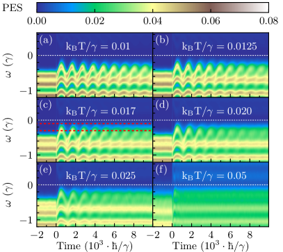
Figure 2: Photoemission spectrum for a chain of $L=30$ sites at different temperatures. The electron-phonon coupling is $\lambda=0.6$ and the phonon frequency is $\Omega=0.01\ \gamma/\hbar$. The pump parameters are $E_{0}=0.33$, $\sigma_{\rm p}=10\ \hbar/\gamma$, and $\omega_{p}=0.1\ \gamma/\hbar$. The thin red dashed lines in panel (c) show the energy range where we average the PES in order to compute the inverted intensity shown in Fig. 3(c).

As observed in experiments (see, e.g., Ref. Schmitt et al., 2008), the lattice motion causes the gap energy to oscillate, which is reflected in the computed PES at low temperatures in Fig. 2. The equilibrium spectrum before the pump is gapped due to the Peierls distortion and only the lower band is populated. After excitation, the system will stabilize to a new equilibrium with a reduced gap energy. Increasing the temperature of the lattice has two major effects on the computed PES. The first is the evident damping of the gap oscillations, so the system relaxes faster to a new equilibrium PES for higher temperatures. The second effect is the "washing out" of the finer details in the spectrum at higher temperatures, increasing at longer times. The period of initial PES oscillations in Fig. 2(a) is much larger (around 1000 $\hbar/\gamma$) than what one would expect for $\Omega=0.01$ $\gamma/\hbar$ which is a clear sign that electron-phonon interaction significantly modifies the intrinsic phonon frequency. The advantage of our self-consistent MC approach is evident from the time scale of Fig. 2, where the time resolution must be kept at $0.1\ \hbar/\gamma$ to capture the electron dynamics, still the fast evolution scheme allows us to average over 3000 MC configurations. Translating these units to the ones in experiments, for $\gamma=1$ eV, the time step is $\Delta t\approx 0.07$ fs, while the simulation time is around 7 ps. For comparison, the time-dependent density-matrix renormalization group method can only reach times on the order of several femtoseconds. Stolpp et al. (2020); Hashimoto and Ishihara (2017); Matsueda et al. (2012)

The internal dynamics captured by the PES in Fig. 2 is also reflected in two order parameters that track the behaviour of the electronic and the lattice subsystem. For the electrons, we define the order parameter via the time-dependent density-density correlation function at the ordering vector $q=\pi$,

$$S_{\rm el}(t)=\frac{1}{L}\sum_{j_{1},j_{2}}(-1)^{j_{1}-j_{2}}\langle\hat{n}_{j_{1}}(t)\hat{n}_{j_{2}}(t)\rangle\,.$$ (8)

For the lattice, we define a similar correlation function of the local lattice displacements,

$$S_{\rm ph}(t)=\frac{1}{L}\sum_{j_{1},j_{2}}(-1)^{j_{1}-j_{2}}\langle\Delta_{j_{1}}(t)\Delta_{j_{2}}(t)\rangle\,.$$ (9)

The oscillations of these two order parameters, shown in Figs. 3(a) and 3(b) for different temperatures, follow the average inverted PES intensity near the gap in Fig. 3(c). As with the PES in Fig. 2, the order parameters are also stabilizing at a new equilibrium, with relaxation times inversely depending on the initial lattice temperature. For each initial temperature in Fig. 3(a), we fit the time dependence of $S_{\rm el}(t)$ with an exponentially decaying function $A\,e^{-t/\tau}\cos(\omega_{\rm f}t)$ to determine the relevant relaxation time $\tau$. The fitted decay times in Fig. 3(d) show that an initially hotter system relaxes faster towards the new equilibrium.

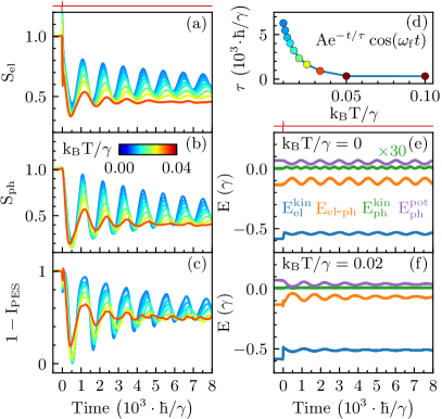
Figure 3: (a), (b) Time evolution of the electron and phonon order parameters $S_{\rm el}(t)$ and $S_{\rm ph}(t)$, as defined in Eqs. (8) and (9), for different initial temperatures (see the colorbar in panel (b)). The order parameters are normalized to one before the pump is applied. (c) Time evolution of the inverse of a normalized in-gap PES intensity (averaged over the energy window between the two red lines in Fig. 2(c)) for the same temperatures as in (a) and (b). (d) Temperature dependence of the relaxation time $\tau$ extracted from panel (a) by fitting $S_{\rm el}(t)$ to the form $Ae^{-t/\tau}\cos(\omega_{\rm f}t)$; the relaxation time diverges as $T\to 0$. (e), (f) Time evolution of the energy expectation values per site of the different contributions in Eqs. (2) and (3), $E_{\rm el}^{\rm kin}$, $E_{\rm el-ph}$, $E_{\rm ph}^{\rm kin}$, and $E_{\rm ph}^{\rm pot}$, at temperatures $k_{\rm B}T=0$ and $k_{\rm B}T=0.02\ \gamma$. Due to the fast electron motion at $T=0$ (due to no relaxation), the electronic energies in panel (e) are time averaged over 50 time steps (with a sliding time window). These time-averaged curves are similar to the nonzero $T$ curves in (f) except they do not get damped. The time profile of the pump field is shown as a thin red curve above the panels (a) and (e). The pump parameters are $\omega_{\rm p}=0.1\ \gamma/\hbar$, $\sigma_{\rm p}=10\ \hbar/\gamma$, $E_{0}=0.33$, while for the phonons $\Omega=0.01\ \gamma/\hbar$ and $\lambda=0.6$.

We observe similar relaxation dynamics for the electron and phonon energies in Fig. 3(f). During relaxation, the electrons exchange kinetic energy with the lattice thus reducing the initial lattice displacement and thereby also the phonon potential energy $E^{\rm pot}_{\rm ph}$. The resulting oscillations in Fig. 3(f) are underdamped. The transfer of energy from electrons to phonons is a slow process, happening on a time scale significantly longer than those determined by relevant electronic and phonon energy scales. Due to the self-consistent nature of our method we are able to predict these nontrivial time scales starting only from a tight-binding Hamiltonian in Eqs. (2) and (3) and without any additional assumptions about the given system. Note that the oscillating behaviour can already be deduced from the zero-temperature results with a sliding time average, as shown in Fig. 3(e), but the dynamics remains undamped and cannot give any insight into relaxation times. Because of this, we apply our method at $T=0$ only to describe the dynamics during or right after the pump excitation, when damping effects are small, and we additionally smooth some of the electronic observables by computing their time averages. Further information on the raw results at $T=0$ are provided in the SI.

We examine the conditions for the weak and strong driving scenarios by modulating the square of the pump amplitude $E_{0}^{2}$ (which is proportional to its fluence) for the two pulse profiles in Figs. 4(a) and 4(b). For the first profile, weak (strong) driving is illustrated in Fig. 4(c) for $E_{0}^{2}=0.1$ ($E_{0}^{2}=0.2$). The inversion of order at $E_{0}^{2}=0.2$ happens in both electronic and lattice subsystems simultaneously. To invert the order, the pump needs to exceed a threshold intensity (marked by the dashed yellow line in Fig. 4(e)). The pump does not invert the order immediately, but it is the coupled dynamics of electrons and phonons which leads to the inversion only at later times (e.g. around 500 $\hbar/\gamma$ for $E^{2}_{0}=0.2$ in Fig. 4(c)), because the lattice moves much slower than the electrons. At the crossover intensity, the phonon amplitude saturates to a constant value (see the inset in Fig. 4(e)) and does not further change with $E_{0}^{2}$. This amplitude saturation as a function of fluence is one of the signatures of order inversion to look for in CDWs but also in other systems with degenerate ground states such as excitonic insulators, as recently demonstrated in Ref. Ning et al., 2020.

We contrast the two driving regimes obtained from the pump in Fig. 4(a) with another pump profile illustrated in Fig. 4(b) which has been used to study CDW melting in Ref. Schmitt et al., 2008. In the melting regime, the electrons are almost instantly driven to a state with charge density oscillating around 1/2 (Fig. 4(d)). The electron-phonon coupling at this point is effectively zero and the electrons and phonons are dynamically decoupled for a period of time. Therefore, phonons will initially oscillate fully harmonically, as a sine wave with periodicity $2\pi/\Omega$ (see Fig. 4(f)), just to be perturbed by the electrons at later times. The dependence on the pump intensity in Figs. 4(e) and 4(f) was computed for $T=0$ because of numerical efficiency. However, the results for low temperatures would be similar because the damping effect caused by the temperature is low in the time range considered in Figs. 4(e) and 4(f). Similar to the electronic energy in Fig. 3(e), the charge density at $T=0$ is time-averaged; for raw data we refer the reader to the SI.

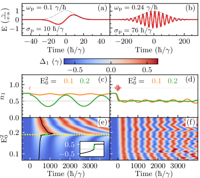
Figure 4: Perturbation of CDW order for a system starting at $k_{\mathrm{B}}T=0$ by a pump. (a), (b) Electric field (red curve) and its envelope function (dotted black curve) for two considered pump profiles: (a) the pump used in Figs. 2 and 3, and (b) a pump with parameters set from Ref. Schmitt et al., 2008. The field is given in units of $\gamma/(e\cdot a)$, where $e$ is the electron charge and $a$ is the lattice constant. (c), (d) Time evolution of the charge density $n_{1}(t)$ on the first site of the chain for the two pump pulses in (a) and (b) and for two different amplitudes. The thin red lines illustrate the time profiles of the two pulses from (a) and (b). The presented charge density is time-averaged over a window of 50 time steps. We refer the reader to the SI for raw $T=0$ results. (e), (f) The time evolution of the phonon displacement $\Delta_{1}(t)$ on the first site of the lattice as a function of the pump intensity $E_{0}^{2}$ for the two pump profiles in (a) and (b), respectively. The dashed yellow line in (e) is the threshold intensity at which the lattice order changes sign. The inset in (e) tracks the amplitude of the first peak in $\Delta_{1}$ as marked with the black curve in (e). The phonon frequency is $\Omega=0.01\gamma/\hbar$, $\lambda=0.6$, and $L=600$.

Discussion

We demonstrated that our time-dependent semi-classical MC modelling captures the experimentally observed dynamics of electron-phonon coupled systems driven out of equilibrium, starting from the initial excitation to the subsequent relaxation at finite temperatures. We have concentrated on an indirect driving mechanism for the lattice dynamics. In future studies, a direct coupling of the lattice to the field may give additional insight into the interplay between indirect and direct driving mechanisms. Moreover, different types of electron-phonon interaction can lead to a periodic lattice distortion accompanied by charge order, which opens up new questions about their pump-probe dynamics. For example, in the Su-Schrieffer-Heeger model Su et al. (1979) the diagonal coupling of lattice displacements and onsite charge density is replaced with an off-diagonal coupling between deviations of neighboring bond length and the neighboring hopping. However, the equations of motion remain of the same form, therefore the indirect driving mechanism revolves around pump driving a local bond current, which modifies the local bond length. Another question is how the indirect driving mechanism is influenced by anharmonic potential terms like $\sum_{i}\Omega_{4}\Delta_{i}^{4}$ considered in Ref. Paleari et al., 2021. Although this term will modify the shape of the potential energy curve for each lattice displacement, the connection between the time-dependent charge density $n_{i}(t)$ and the local displacement minima still exists. In addition, this approach can be directly extended to two dimensions, Weber and Freericks (2022) but with additional computational cost.

Our explanation of the indirect driving in terms of the modification of the local lattice potential and the reduction of the energy barrier is very similar to the standard phenomenological Ginzburg-Landau (GL) model, often employed to explain trARPES experiments. The GL model predicts a double-well structure in the free-energy potential, which upon excitation with a strong pump can turn into a single-well potential where the order parameter oscillates around zero. Maklar et al. (2021) Here, we propose an efficient complementary approach to GL, which allows for a more detailed microscopic exploration with consideration of the full Hamiltonian of the system, but without the computational cost of a more demanding first-principles method such as for example time-dependent density functional theory. We view our method as a balanced alternative which offers a way to self-consistently induce lattice motion by direct coupling with the pump field and to evolve the system to timescales relevant for phonon effects to appear. The damping of the phonon oscillations emerges naturally from our finite-temperature method, without the need to modify the lattice equations of motion in order to include damping. Another important characteristic of our time evolution scheme is that it produces a true nonequilibrium electronic state, without any additional assumptions regarding the time scales it takes for electrons to thermalize. This opens up the possibility to examine many different types of pump-probe experiments.

The inversion of the lattice order, accompanied by the inversion of electronic charge density ordering, is not a specific feature of just CDW systems. A similar mechanism was recently reported and measured in excitonic insulators. Ning et al. (2020) A double pump pulse was used to modulate the phonon oscillations and suppress or enhance the phonon amplitude, and the enhancement was related to the inverted structural order. A similar modulation of the phonon amplitude was also reported for tritellurides, Rettig et al. (2014) although it was not directly associated with the inversion of order. The possibility to invert the order appears to be a general feature of all systems with degenerate ground states coupled with the lattice. An interesting feature of the order inversion is that a system can briefly pass through a metastable state where electrons and phonons are decoupled, so the inversion of order is accompanied with a state that might have dramatically different conductivity.

Materials and Methods

At $T=0$, the perfectly-dimerized state with $\Delta_{0,i}=(-1)^{i}\Delta$ remains a static solution of the equations of motion if no field is applied, whereas our MC averaged quantities at $T>0$ require a thermalization period before we apply the pump. For all our simulations, we use a time step of $\Delta t=0.1\ \hbar/\gamma$ which is set by the fast electron dynamics.

The pump field modifies the phase $\varphi(t)$ of the nearest-neighbor hopping in Eq. (2) through the time-dependent vector potential $\mathbf{A}(\mathbf{r},t)=-c\int^{t}\mathbf{E}(\mathbf{r},t^{\prime})\,dt^{\prime}$; a spatially homogeneous field essentially shifts the electron momentum. We work in the gauge where the time-dependent scalar potential $\Phi(\mathbf{r},t)$ is zero.

The time-dependent PES is computed according to Ref. Freericks et al., 2009,

$$P(\omega,t)= -i\int_{-\infty}^{\infty}dt_{1}\int_{\infty}^{\infty}dt_{2}\,s(t_{1}-t)s(t_{2}-t)e^{-i\omega(t_{1}-t_{2})}$$

$$\times\frac{1}{L}\sum_{i=1}^{L}G^{<}_{ii}(t_{1},t_{2})\,,$$ (10)

where $G^{<}_{ii}(t_{1},t_{2})=i\langle\hat{c}_{i}^{\dagger}(t_{2})\hat{c}_{i}(t_{1})\rangle$ is the time-displaced local lesser Green’s function and $s(t)=\exp\left[-{t^{2}}/{2{\sigma}^{2}_{\rm probe}}\right]/\sqrt{2\pi}\sigma_{\rm probe}$ is the shape of the probe pulse of width $\sigma_{\rm probe}=10\ {\rm\hbar/\gamma}$ centered at $t=0$.

Supporting Information Appendix: Theoretical description of time-resolved photoemission in charge-density-wave materials out to long times

Quantum versus classical harmonic oscillator

The quantum and classical harmonic oscillators are closely related to each other, especially if the harmonic oscillator has a large average energy. We state some of the facts about the quantum and classical oscillator that show this relationship.

First, if the quantum state is described via a coherent state, then the time dependence of the average position and the momentum of the quantum oscillator are identical to that of a classical pulled mass on a spring. Second, if we compute the product of the fluctuations about the mean of the position and momentum over a period of oscillation for a classical harmonic oscillator it is given by $E/\Omega$, which is exactly what the quantum state uncertainty product is for energy eigenstates—the major difference is that the quantum oscillator only has an allowed set of energies. Third, if the average energy of the oscillator is larger than the phonon frequency, then the difference between the quantum and classical expectation values become quite small and decrease as the average energy increases. The main difference is that a classical oscillator can have energies smaller than $\frac{1}{2}\hbar\Omega$, and the fluctuations in position and momentum then both go to zero. This is clearly quite different from that of the quantum oscillator. Hence, in situations where the oscillator has a relatively large average energy, as compared to $\hbar\Omega$, the semiclassical approximation for the electron-phonon coupled problem should be quite accurate. This should always occur when one pumps significant energy into a system to drive it to nonequilibrium, as we do in the work presented here.

Photoemission at zero temperature

As already stated in the main text, results for zero temperature are limited because they do not show any damping, and once the system is excited, it will continue to oscillate indefinitely. The photoemission spectrum at $T=0$ is presented in Fig. S1 The dynamics of energy levels reveals the gap centered at $\omega=0$ which is modulated by the symmetric motion of the upper and the lower band, a behaviour previously observed experimentally. Rettig et al. (2014) Note that the discreteness of the spectra in Fig. S1 is due to limited lattice sizes. We verify that $L=30$ sites are sufficient to reliably estimate the oscillating gap and that the PES becomes continuous for $L=100$, as shown on the right of Fig. S1.

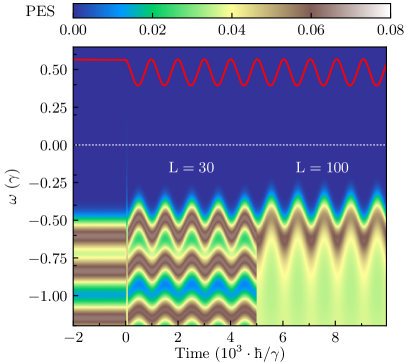
Figure S1: The photoemission spectrum at $T=0$ temperature. Data for times below $5\cdot 10^{3}\rm\ \hbar/\gamma$ is obtained for a system with $L=30$ sites, while data above this time is obtained using a system with $L=100$ sites. The red curve shows the oscillations of the phonon displacement, which corresponds to the gap energy $\Delta(t)$. Other parameters are the same as those used in Fig. 2 in the main text: $\Omega=0.01\ \gamma/\hbar$, $\lambda=0.6$, $E_{0}=0.33$, $\sigma_{\rm p}=10\ \hbar/\gamma$, $\omega_{\rm p}=0.1\ \gamma/\hbar$.

The raw data for the electronic energies at $T=0$ presented in Fig. 3 in the main text is shown in Fig. S2, while the raw data for the charge density excitation for the weak and strong pump shown in Figs. 4(c) and 4(d) in the main text are shown in the corresponding Figs. S3(a), S3(c), and S3(b), S3(d) respectively.

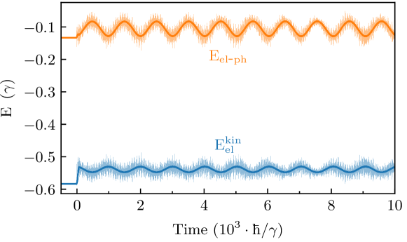
Figure S2: Raw $T=0$ results for the electron kinetic and potential energy (transparent background) and the corresponding time-averaged results (full color curves) originally presented in Fig. 3(e) in the main text. The system parameters are: $L=30$, $\lambda=0.6$, $\Omega=0.01\ \gamma/\hbar$, $E_{0}=0.33$, $\omega_{\rm p}=0.1\ \gamma/\hbar$, and $\sigma_{\rm p}=10\ \hbar/\gamma$.

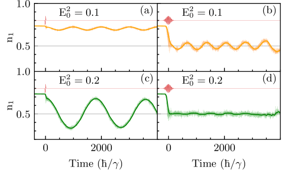
Figure S3: Weak and strong pump driving at $T=0$ temperature. Full color curves in (a), (c) and (b), (d) correspond to time-averaged oscillations of the charge density at the first site of the system, originally presented in Figs. 4(c) and 4(d) in the main text (for pump amplitudes $E^{2}_{0}=0.1$ and $E^{2}_{0}=0.2$), respectively. The transparent background shows the raw data before the time averaging. Other system parameters are: $L=600$, $\lambda=0.6$, $\Omega=0.01\ \gamma/\hbar$. The system in (a) and (c) is excited using a pump with $\omega_{\rm p}=0.1\ \gamma/\hbar$, $\sigma_{\rm p}=10\ \hbar/\gamma$, while that in (b), and (d) is excited with a pump with $\omega_{\rm p}=0.24\ \gamma/\hbar$, $\sigma_{\rm p}=76\ \hbar/\gamma$.

Figures S4 and S5 additionally explain the data presented in the three supplementary videos.

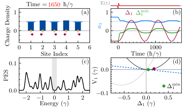
Figure S4: Explanation of the data presented in the two supplementary movies (Video 1 and Video 2): (a) Local charge density $n_{i}(t)$ (dark blue bars) on the first five sites (orange dots). The lattice displacements $\Delta_{i}(t)$ (dark red dots and dark lines below the orange dots) are scaled from their original values to values below one half in order to fit them between the neighboring sites. Light blue horizontal lines above the blue bars emphasize the charge density $n_{i}(t)$ on odd sites. (b) Time-dependence of the phonon displacement $\Delta_{1}(t)$ (the dark-red curve), the minimal displacement determined from the potential energy $\Delta_{1}^{\min}(t)$ (the green curve) and the time-averaged charge density $n_{1}(t)$ (the light blue curve) on the first site (and all odd sites). (c) The intensity of the photoemission spectrum. The gray rectangle at the center shows the expected gap size obtained from $\Delta_{1}(t)$. (d) The potential energy profile for the first site $V_{1}(\Delta_{1}(t))$. The dark-red dot shows the actual position $\Delta_{1}(t)$ while the green dot show the $\Delta_{1}^{\min}(t)$. The dashed light blue line shows the tangent of the energy parabola determined from the first derivative $n_{1}(t)-1/2$, the gray parabola in the background shows the energy profile in equilibrium before the pump. The electron charge density is time-averaged over 50 time steps.

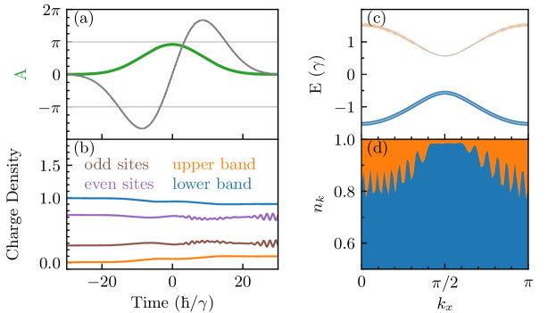
Figure S5: Explanation of the data presented in the Video 3: Time evolution of the electron occupation numbers in the upper and lower bands. (a) The time profile of the vector potential intensity ${A}(t)$ (the green curve) and the pump field $E(t)$ (the gray curve). (b) The time profile of the average charge density on all even sites (the violet curve) and all the odd sites (the brown curve) in real space. The corresponding Fourier transformed values show the time profiles of the electron occupation numbers in the lower band (the blue curve) and in the upper band (the orange curve). (c) $k$-resolved occupation of the upper and lower bands. The transparency of the blue and orange curves corresponds to the occupation number for a given $k$ (full transparent equals to zero occupation). (d) Graphical representation of the $k$-resolved occupation shown in (c). The orange surface corresponds to the upper band, while the blue surface corresponds to the lower band. Since the vector potential shifts the electron momentum, we translate the results in (c) and (d) with $\mathbf{A}(t)$ to keep them gauge invariant.

Video 1: Time evolution of the electronic and the lattice system for the weak pump at $k_{\rm B}T=0$ temperature. The presented data is obtained for $T=0$ temperature because of numerical efficiency. The fast oscillations of the charge density are expected to average to smooth curves for $T>0$ which would be closer to the presented time-averaged $n_{1}(t)$. We have verified this by doing calculations at a finite temperature as seen by comparing Fig. 3(e) and Fig. 3(f) in the main text. Parameters used are $E_{0}=0.33$, $\lambda=0.6$, $\sigma_{\rm p}=10\ \hbar/\gamma$, $\omega_{\rm p}=0.1\ \gamma/\hbar$, $\Omega=0.01\ \gamma/\hbar$, $\gamma=1$, $L=30$.

Video 2: Time evolution of the electronic and the lattice system for the strong pump at $k_{\rm B}T=0$ temperature. The presented data is obtained for $T=0$ temperature because of numerical efficiency. The fast oscillations of the charge density are expected to average to smooth changes for $T>0$ which would be closer to the presented time-averaged $n_{1}(t)$. Parameters used are $E_{0}=0.66$, $\lambda=0.6$, $\sigma_{\rm p}=10\ \hbar/\gamma$, $\omega_{\rm p}=0.1\ \gamma/\hbar$, $\Omega=0.01\ \gamma/\hbar$, $\gamma=1$, $L=30$.

Video 3: Electron dynamics in $k$-space during the pump excitation at $k_{\rm B}T=0$. Here, $E_{0}=0.4$, $\Omega=0$, $\lambda=0.6$, $\sigma_{\rm p}=10\ \hbar/\gamma$, $\omega_{\rm p}=0.1\ \gamma/\hbar$, $\gamma=1$.

References

- Sobota et al. (2021) J. A. Sobota, Y. He, and Z.-X. Shen, Rev. Mod. Phys. 93, 025006 (2021).
- Gerber et al. (2017) S. Gerber, S.-L. Yang, D. Zhu, H. Soifer, J. A. Sobota, S. Rebec, J. J. Lee, T. Jia, B. Moritz, C. Jia, A. Gauthier, Y. Li, D. Leuenberger, Y. Zhang, L. Chaix, W. Li, H. Jang, J.-S. Lee, M. Yi, G. L. Dakovski, S. Song, J. M. Glownia, S. Nelson, K. W. Kim, Y.-D. Chuang, Z. Hussain, R. G. Moore, T. P. Devereaux, W.-S. Lee, P. S. Kirchmann, and Z.-X. Shen, Science 357, 71 (2017).
- Aeschlimann et al. (2021) S. Aeschlimann, S. A. Sato, R. Krause, M. Chávez-Cervantes, U. De Giovannini, H. Hübener, S. Forti, C. Coletti, K. Hanff, K. Rossnagel, A. Rubio, and I. Gierz, Nano Letters 21, 5028 (2021).
- Sobota et al. (2012) J. A. Sobota, S. Yang, J. G. Analytis, Y. L. Chen, I. R. Fisher, P. S. Kirchmann, and Z.-X. Shen, Phys. Rev. Lett. 108, 117403 (2012).
- Gruner (1994) G. Gruner, Density Waves In Solids (Basic Books, 1994).
- Grüner (1988) G. Grüner, Rev. Mod. Phys. 60, 1129 (1988).
- Perfetti et al. (2006) L. Perfetti, P. A. Loukakos, M. Lisowski, U. Bovensiepen, H. Berger, S. Biermann, P. S. Cornaglia, A. Georges, and M. Wolf, Phys. Rev. Lett. 97, 067402 (2006).
- Perfetti et al. (2008) L. Perfetti, P. A. Loukakos, M. Lisowski, U. Bovensiepen, M. Wolf, H. Berger, S. Biermann, and A. Georges, New. J. Phys 10, 053019 (2008).
- Schmitt et al. (2008) F. Schmitt, P. S. Kirchmann, U. Bovensiepen, R. G. Moore, L. Rettig, M. Krenz, J.-H. Chu, N. Ru, L. Perfetti, D. H. Lu, M. Wolf, I. R. Fisher, and Z.-X. Shen, Science 321, 1649 (2008).
- Schmitt et al. (2011) F. Schmitt, P. S. Kirchmann, U. Bovensiepen, R. G. Moore, J.-H. Chu, D. H. Lu, L. Rettig, M. Wolf, I. R. Fisher, and Z.-X. Shen, New. J. Phys. 13, 063022 (2011).
- Maklar et al. (2021) J. Maklar, Y. W. Windsor, C. W. Nicholson, M. Puppin, P. Walmsley, V. Esposito, M. Porer, J. Rittmann, D. Leuenberger, M. Kubli, M. Savoini, E. Abreu, S. L. Johnson, P. Beaud, G. Ingold, U. Staub, I. R. Fisher, R. Ernstorfer, M. Wolf, and L. Rettig, Nat. Commun. 12, 2499 (2021).
- Kogar et al. (2020) A. Kogar, A. Zong, P. E. Dolgirev, X. Shen, J. Straquadine, Y.-Q. Bie, X. Wang, T. Rohwer, I.-C. Tung, Y. Yang, R. Li, J. Yang, S. Weathersby, S. Park, M. E. Kozina, E. J. Sie, H. Wen, P. Jarillo-Herrero, I. R. Fisher, X. Wang, and N. Gedik, Nature Physics 16, 159 (2020).
- Zong et al. (2021) A. Zong, P. E. Dolgirev, A. Kogar, Y. Su, X. Shen, J. A. W. Straquadine, X. Wang, D. Luo, M. E. Kozina, A. H. Reid, R. Li, J. Yang, S. P. Weathersby, S. Park, E. J. Sie, P. Jarillo-Herrero, I. R. Fisher, X. Wang, E. Demler, and N. Gedik, Phys. Rev. Lett. 127, 227401 (2021).
- Hübener et al. (2018) H. Hübener, U. De Giovannini, and A. Rubio, Nano Letters 18, 1535 (2018).
- Moritz et al. (2010) B. Moritz, T. P. Devereaux, and J. K. Freericks, Phys. Rev. B 81, 165112 (2010).
- Matveev et al. (2016) O. P. Matveev, A. M. Shvaika, T. P. Devereaux, and J. K. Freericks, Phys. Rev. B 94, 115167 (2016).
- Shen et al. (2014a) W. Shen, T. P. Devereaux, and J. K. Freericks, Phys. Rev. B 90, 195104 (2014a).
- Shen et al. (2014b) W. Shen, Y. Ge, A. Y. Liu, H. R. Krishnamurthy, T. P. Devereaux, and J. K. Freericks, Phys. Rev. Lett. 112, 176404 (2014b).
- Freericks et al. (2017) J. K. Freericks, O. P. Matveev, W. Shen, A. M. Shvaika, and T. P. Devereaux, Phys. Scr. 92, 034007 (2017).
- De Filippis et al. (2012) G. De Filippis, V. Cataudella, E. A. Nowadnick, T. P. Devereaux, A. S. Mishchenko, and N. Nagaosa, Phys. Rev. Lett. 109, 176402 (2012).
- Matsueda et al. (2012) H. Matsueda, S. Sota, T. Tohyama, and S. Maekawa, Journal of the Physical Society of Japan 81, 013701 (2012).
- Hashimoto and Ishihara (2017) H. Hashimoto and S. Ishihara, Phys. Rev. B 96, 035154 (2017).
- Stolpp et al. (2020) J. Stolpp, J. Herbrych, F. Dorfner, E. Dagotto, and F. Heidrich-Meisner, Phys. Rev. B 101, 035134 (2020).
- Sous et al. (2021) J. Sous, B. Kloss, D. M. Kennes, D. R. Reichman, and A. J. Millis, Nature Communications 12 (2021).
- Abedi et al. (2010) A. Abedi, N. T. Maitra, and E. K. U. Gross, Phys. Rev. Lett. 105, 123002 (2010).
- Lively et al. (2021) K. Lively, G. Albareda, S. A. Sato, A. Kelly, and A. Rubio, The Journal of Physical Chemistry Letters 12, 3074 (2021), pMID: 33750137.
- Weber and Freericks (2022) M. Weber and J. K. Freericks, Phys. Rev. E 105, 025301 (2022).
- Car and Parrinello (1985) R. Car and M. Parrinello, Phys. Rev. Lett. 55, 2471 (1985).
- Brazovskii and Dzyaloshinskii (1976) S. A. Brazovskii and I. E. Dzyaloshinskii, Zh. Eksp. Teor. Fiz. 71, 2338 (1976).
- Weber et al. (2018) M. Weber, F. F. Assaad, and M. Hohenadler, Phys. Rev. B 98, 235117 (2018).
- Freericks et al. (2009) J. K. Freericks, H. R. Krishnamurthy, and T. Pruschke, Phys. Rev. Lett. 102, 136401 (2009).
- Weber et al. (2016) M. Weber, F. F. Assaad, and M. Hohenadler, Phys. Rev. B 94, 155150 (2016).
- Ning et al. (2020) H. Ning, O. Mehio, M. Buchhold, T. Kurumaji, G. Refael, J. G. Checkelsky, and D. Hsieh, Phys. Rev. Lett. 125, 267602 (2020).
- Su et al. (1979) W. P. Su, J. R. Schrieffer, and A. J. Heeger, Phys. Rev. Lett. 42, 1698 (1979).
- Paleari et al. (2021) G. Paleari, F. Hébert, B. Cohen-Stead, K. Barros, R. Scalettar, and G. G. Batrouni, Phys. Rev. B 103, 195117 (2021).
- Rettig et al. (2014) L. Rettig, J.-H. Chu, I. R. Fisher, U. Bovensiepen, and M. Wolf, Faraday Discuss. 171, 299 (2014).