Exponential Convergence of $hp$-Time-Stepping
in Space-Time Discretizations of Parabolic PDEs

Abstract.

For linear parabolic initial-boundary value problems with self-adjoint, time-homogeneous elliptic spatial operator in divergence form with Lipschitz-continuous coefficients, and for incompatible, time-analytic forcing term in polygonal/polyhedral domains $\mathrm{D}$, we prove time-analyticity of solutions. Temporal analyticity is quantified in terms of weighted, analytic function classes, for data with finite, low spatial regularity and without boundary compatibility. Leveraging this result, we prove exponential convergence of a conforming, semi-discrete $hp$-time-stepping approach. We combine this semi-discretization in time with first-order, so-called “$h$-version” Lagrangian Finite Elements with corner-refinements in space into a tensor-product, conforming discretization of a space-time formulation. We prove that, under appropriate corner- and corner-edge mesh-refinement of $\mathrm{D}$, error vs. number of degrees of freedom in space-time behaves essentially (up to logarithmic terms), to what standard FEM provide for one elliptic boundary value problem solve in $\mathrm{D}$. We focus on two-dimensional spatial domains and comment on the one- and the three-dimensional case.

AMS Subject Classification: primary 65N30

1. Introduction

Efficient numerical solution of parabolic evolution problems is required in many applications. In addition to the plain numerical solution of associated initial-boundary value problems, in recent years the efficient numerical treatment of optimal control problems and of uncertain input data has been considered. Here, often a large number of cases needs to be treated, and the (numerical) solution must be stored in a data-compressed format. Rather than the (trivial) option of a posteriori compressing a numerical solution obtained by a standard scheme, novel algorithms have emerged featuring some form of space-time compressibility in the numerical solution process. I.e., the numerical scheme will obtain directly, at runtime, a numerical solution in a compressed format. As examples, we mention only sparse-grid and wavelet-based methods (e.g., [18]), and wavelet-based compressive schemes (e.g., [19, 30] and the references there). Key to successful compressive space-time discretizations is an appropriate variational formulation of the evolution problem under consideration. Accordingly, recent years have seen the development of a variety of, in general nonequivalent, space-time variational formulations of parabolic initial-boundary value problems. Departing from the classical, Bochner-space perspective used to establish well-posedness, the novel formulations adopt the perspective of treating the parabolic evolution problem as an operator equation between appropriate function spaces, the primary motivation being accomodation of efficient, compressive space-time numerical schemes. We mention only [30, 3, 32, 20, 9, 34, 25, 14, 15, 36] and the references there. A comprehensive account of the numerical analysis of fixed order time-discretizations is provided in [37] and the references there. In the results given in that volume, the semigroup perspective is adopted, and the mathematical setting is based on homogeneous Sobolev spaces $\dot{H}^{s}(\mathrm{D})$, which impose implicit boundary compatibilities of regular data, see [37, Chapter 19].

The presently investigated time-discretization approach is based on the space-time variational formulation in [34]. It is of Petrov–Galerkin type, and is based on a fractional order Sobolev space in the temporal direction. It has been proposed and developed in a series of papers [34, 35, 39, 21, 33]. We briefly recapitulate it here, and refer to [34] for full development of details. The compressive aspect is here realized by the $hp$-time discretization for this formulation.

Throughout, we denote by $\mathrm{D}\subset\mathbb{R}^{d}$ a bounded interval (if $d=1$), or a bounded polygonal (if $d=2$) or polyhedral (if $d=3$) domain, with a Lipschitz boundary $\Gamma=\partial\mathrm{D}$ consisting of a finite number of plane faces, and by $T>0$ a finite time horizon. In the space-time cylinder $Q=(0,T)\times\mathrm{D}$, we consider the parabolic initial-boundary value problem (IBVP for short) governed by the partial differential equation

(1.1) $$Bu:=\partial_{t}u+A(\partial_{x})u=g\quad\mbox{in}\quad(0,T)\times\mathrm{D}.$$

Here, the forcing function $g:Q\to\mathbb{R}$ is assumed to belong to $\mathcal{A}([0,T];L^{2}(\mathrm{D}))$, i.e., it is analytic as a map from $[0,T]$ into $L^{2}(\mathrm{D})$. The spatial differential operator $A(\partial_{x})$ is assumed linear, self-adjoint, in divergence form, i.e.,

$$A(\partial_{x})=-\nabla_{x}\cdot(A(x)\nabla_{x})$$

with $A\in L^{\infty}(\mathrm{D};\mathbb{R}^{d\times d})$ being a symmetric, positive definite matrix function of $x\in\mathrm{D}$ which does not depend on the temporal variable $t$. The PDE (1.1) is completed by initial condition

(1.2) $$u|_{t=0}=u_{0}\;,$$

and by mixed boundary conditions

(1.3) $$\gamma_{0}(u)=u_{D}\quad\mbox{on}\quad\Gamma_{D}\;,\quad\gamma_{1}(u)=u_{N}\quad\mbox{on}\quad\Gamma_{N}\;.$$

Here, $\Gamma_{D}$ and $\Gamma_{N}$ denote a partitioning of $\Gamma=\partial\mathrm{D}$ into a Dirichlet and a Neumann part, $\gamma_{0}$ denotes the Dirichlet trace map, and $\gamma_{1}$ denotes the conormal trace operator, given (in strong form) by $\gamma_{1}(v)=n_{x}\cdot(A(x)\nabla_{x}v)|_{\Gamma}$, with $\Gamma=\partial\mathrm{D}$ denoting the boundary of $\mathrm{D}$, and $n_{x}\in L^{\infty}(\Gamma;\mathbb{R}^{d})$ the exterior unit normal vector field on $\Gamma$.

Remark 1.1.

In the rest of this paper, the results are formulated for $u_{0}=0$, $u_{D}=0$, and $u_{N}=0$. Since the IBVP (1.1)–(1.3) is linear, superposition for a sufficiently regular function $U(x,t)$ in $Q$, which satisfies (1.2) and (1.3), will imply that the function $u-U$ will solve (1.1)–(1.3) with $g-BU$ in place of $g$ in (1.1), and with homogeneous initial and boundary data in (1.2) and (1.3). All regularity hypotheses which we will impose below on the source term $g$ in (1.1) (in particular, time-analyticity (3.9)) entail via $U$ corresponding assumptions on $u_{0}$, $u_{D}$, and $u_{N}$.

Exploiting the analytic semigroup property of the parabolic evolution operator, we provide in Section 3.1 sufficient conditions for the time analyticity of solutions when considered as maps from the time interval $[0,T]$ into a suitable Sobolev space $W\subset L^{2}(\mathrm{D})$ on the bounded spatial domain $\mathrm{D}\subset\mathbb{R}^{d}$.

Contributions of the present paper are a weighted analytic, temporal regularity analysis based on the analytic semigroup theory for linear, parabolic evolution equations, for source terms and coefficients of finite spatial regularity, and the proof of exponential convergence of a temporal $hp$-discretization. For polygonal spatial domain $\mathrm{D}\subset\mathbb{R}^{2}$, and for data without boundary compatibility, we establish a priori convergence rate bounds for fully discrete, space-time approximations which are based on a fractional order space-time formulation, on $hp$-time-stepping and on $h$-FEM with corner-refined, regular graded triangulations in $\mathrm{D}$. The diffusion coefficient $A(x)$ is assumed to be independent of $t$, and to belong to $W^{1,\infty}(\mathrm{D};\mathbb{R}^{2\times 2})$. We comment on the cases $d=1$ (when $\mathrm{D}$ is a bounded interval) and $d=3$ (when $\mathrm{D}$ is a polyhedron).

The layout of this paper is as follows: In Section 2, we introduce notation and function spaces of tensor product and of Bochner type, which will be used in the following. We also provide the space-time variational formulation in fractional order spaces and the subspaces used in discretization. Section 3 addresses the solution regularity, with particular attention to temporal analytic regularity in weighted, analytic Bochner spaces of functions taking values in corner-weighted, Kondrat’ev type spaces on the domain $\mathrm{D}$. Section 4 then introduces the Galerkin approximations in space and time that will be used, and their approximation properties. Section 5 contains the main results on the convergence rate of the discretization. Section 6 describes the numerical realization of the nonlocal temporal bilinear form, and reports numerical results which are in full agreement with the convergence rate analysis.

We use standard notation: $\mathbb{N}=\{1,2,\dots\}$ shall denote the natural numbers, and $\mathbb{N}_{0}:=\mathbb{N}\cup\{0\}$. For Banach spaces $X$ and $Y$, $\mathcal{L}(X,Y)$ denotes the space of bounded linear operators from $X$ to $Y$, and $X^{\prime}:=\mathcal{L}(X,\mathbb{R})$ denotes the dual of $X$. For $q\in[1,\infty]$, the usual notation $L^{q}(\mathrm{D})$ is adopted for Lebesgue spaces of $q$-integrable functions $u:\mathrm{D}\to\mathbb{R}$ over some (bounded) domain $\mathrm{D}$ in the Euclidean space $\mathbb{R}^{d}$. For nonnegative integers $k$, Hilbertian Sobolev spaces (where $q=2$) on such domains $\mathrm{D}$ are denoted by $H^{k}(\mathrm{D})$. For $k=0$, as usual, $H^{0}(\mathrm{D})=L^{2}(\mathrm{D})$. Hilbertian Sobolev spaces of noninteger order $s=k+\theta$ for $k\in\mathbb{N}_{0}$ and $0<\theta<1$ are defined by interpolation (real method, with fine index $2$).

2. Function Spaces and Space-time Variational Formulation

We introduce several Bochner-type Sobolev spaces in the space-time cylinder $Q:=J\times\mathrm{D}$, with the finite time interval $J:=(0,T)$ and the bounded spatial domain $\mathrm{D}\subset\mathbb{R}^{d}$.

2.1. Function Spaces

Bochner-type function spaces defined on the space-time cylinder $Q=J\times\mathrm{D}$ are spaces of strongly measurable maps $u\colon\,J\to H^{l}(\mathrm{D})$, such that $u\in H^{k}(J;H^{l}(\mathrm{D}))$ for nonnegative integers $k$,$l$. Due to the Hilbertian structure of $H^{k}$, these separable Hilbert spaces admit tensor product structure, i.e.,

$$H^{k}(J;H^{l}(\mathrm{D}))\simeq H^{k}(J)\otimes H^{l}(\mathrm{D})\simeq H^{l}(\mathrm{D};H^{k}(J))\;,$$

where $\simeq$ denotes (isometric) isomorphism and $\otimes$ the Hilbertian tensor product.

For any integer $k\geq 1$, we denote by $H^{k}_{0}$ the closed subspace of $H^{k}$ of functions with homogeneous boundary values in the sense of closure of $C^{\infty}_{0}$ with respect to the norm of $H^{k}$. For instance, $H^{1}_{0}$ denotes the closed nullspace of the Dirichlet trace operator $\gamma_{0}$.

To consider mixed boundary value problems on $\mathrm{D}$, we partition $\Gamma=\partial\mathrm{D}$ into two disjoint pieces $\Gamma_{D}$ and $\Gamma_{N}$. Assuming positive $(d-1)$-dimensional measure of $\Gamma_{D}$ if $d=2,3$, or that $\Gamma_{D}$ contains at least one endpoint of $D$ if $d=1$, we set

$$H^{1}_{\Gamma_{D}}(\mathrm{D}):=\{v\in H^{1}(\mathrm{D})|\ \gamma_{0}(v)_{\mid_{\Gamma_{D}}}=0\}\;.$$

Evidently, for $\Gamma_{D}\subset\Gamma$, $H^{1}_{0}(\mathrm{D})=H^{1}_{\Gamma}(\mathrm{D})\subset H^{1}_{\Gamma_{D}}(\mathrm{D})\subset H^{1}(\mathrm{D})$.

In the following, we introduce Sobolev spaces for functions defined on an interval $(a,b)\subset\mathbb{R}$ with $a<b$. For simplicity, we consider real-valued functions $v\colon\,(a,b)\to\mathbb{R}$. All results and proofs can be generalized straightforwardly to $X$-valued functions $v\colon\,(a,b)\to X$ for a Hilbert space $X$, i.e., Bochner–Sobolev spaces. We write

$$\begin{split}H^{1}_{0,}(a,b)&=H^{1}_{\{a\}}(a,b)=\{v\in H^{1}(a,b)|\ v(a)=0\},\\ H^{1}_{,0}(a,b)&=H^{1}_{\{b\}}(a,b)=\{v\in H^{1}(a,b)|\ v(b)=0\}\;.\end{split}$$

In either of these two spaces, the seminorm $|\circ|_{H^{1}(a,b)}=\|\partial_{t}\circ\|_{L^{2}(a,b)}$ is a norm. Thus, $|\circ|_{H^{1}(a,b)}$ is considered as the norm in $H^{1}_{0,}(a,b)$ and $H^{1}_{,0}(a,b)$, whereas the space $H^{1}(a,b)$ is endowed with the norm $\|\circ\|_{H^{1}(a,b)}=(\|\circ\|_{L^{2}(a,b)}^{2}+\|\partial_{t}\circ\|_{L^{2}(a,b)}^{2})^{1/2}$.

Fractional order spaces shall be defined by interpolation, via the real method of interpolation (see, e.g., [38, Chapter 1]). We use the fine index $q=2$ to preserve the Hilbertian structure. Of particular interest will be the space

$$H^{1/2}_{0,}(a,b):=(H^{1}_{0,}(a,b),L^{2}(a,b))_{1/2,2}\;,$$

where $|\circ|_{H^{1}(a,b)}=\|\partial_{t}\circ\|_{L^{2}(a,b)}$ is the norm of the space $H^{1}_{0,}(a,b)$. The Sobolev space $H^{1/2}_{0,}(a,b)$ is a Hilbert space endowed with the interpolation norm (see [34, Section 2.3] for $(a,b)=(0,T)$) defined by

(2.1) $$\|v\|_{H^{1/2}_{0,}(a,b)}:=\left(\sum_{k=0}^{\infty}\frac{\pi(2k+1)}{2(b-a)}|v_{k}|^{2}\right)^{1/2},\quad v\in H^{1/2}_{0,}(a,b),$$

where the Fourier coefficients $v_{k}$ are given by $v_{k}=\int_{a}^{b}v(s)V_{k}(s)\mathrm{d}s\;.$ Here, we use that any $z\in L^{2}(a,b)$ admits a representation as a Fourier series

(2.2) $$z(t)=\sum_{k=0}^{\infty}z_{k}V_{k}(t),\quad z_{k}=\int_{a}^{b}z(s)V_{k}(s)\mathrm{d}s,\;k\in\mathbb{N}_{0},$$

where $V_{k}$ denotes an eigenfunction corresponding to eigenvalue $\lambda_{k}=\frac{\pi^{2}(2k+1)^{2}}{4(b-a)^{2}}$ of

(2.3) $$-\partial_{tt}V_{k}(t)=\lambda_{k}V_{k}(t)\;\text{ for }t\in(a,b),\quad V_{k}(a)=\partial_{t}V_{k}(b)=0,\quad{\left\lVert{V_{k}}\right\rVert}_{L^{2}(a,b)}=1.$$

In particular for $J=(0,T)=(a,b)$, we have

$$\|v\|_{H^{1/2}_{0,}(J)}=\left(\frac{\pi}{2T}\sum_{k=0}^{\infty}(2k+1)|v_{k}|^{2}\right)^{1/2},\quad v\in H^{1/2}_{0,}(J),$$

with the Fourier representation

(2.4) $$v(t)=\sum_{k=0}^{\infty}v_{k}\sqrt{\frac{2}{T}}\sin\left(\left(\frac{\pi}{2}+k\pi\right)\frac{t}{T}\right),\;v_{k}=\int_{0}^{T}v(s)\sqrt{\frac{2}{T}}\sin\left(\left(\frac{\pi}{2}+k\pi\right)\frac{s}{T}\right)\mathrm{d}s.$$

Analogous to $H^{1/2}_{0,}(J)$, the Hilbert space $H^{1/2}_{,0}(J):=(H^{1}_{,0}(J),L^{2}(J))_{1/2,2}$ is endowed with the Hilbertian norm (see [34, Section 2.3]) defined by

$$\|w\|_{H^{1/2}_{,0}(J)}:=\left(\frac{\pi}{2T}\sum_{k=0}^{\infty}(2k+1)|w_{k}|^{2}\right)^{1/2},\quad w\in H^{1/2}_{,0}(J),$$

where the Fourier coefficients are given by $w_{k}=\int_{0}^{T}w(s)\sqrt{\frac{2}{T}}\cos\left(\left(\frac{\pi}{2}+k\pi\right)\frac{s}{T}\right)\mathrm{d}s.$

To prove exponential convergence of a temporal $hp$-discretization, we need further investigations of the Sobolev space $H^{1/2}_{0,}(a,b)$ and its norm $\|\circ\|_{H^{1/2}_{0,}(a,b)}$. For this purpose, let the classical Sobolev space $H^{1/2}(a,b)$ be endowed with the Slobodetskii norm [24, p. 74]

(2.5) $${\left|\kern-1.07639pt\left|\kern-1.07639pt\left|v\right|\kern-1.07639pt\right|\kern-1.07639pt\right|}_{H^{1/2}(a,b)}:=\left(\|v\|_{L^{2}(a,b)}^{2}+|v|_{H^{1/2}(a,b)}^{2}\right)^{1/2}$$

for $v\in H^{1/2}(a,b)$ with

(2.6) $$|v|_{H^{1/2}(a,b)}:=\left(\int_{a}^{b}\int_{a}^{b}\frac{|v(s)-v(t)|^{2}}{|s-t|^{2}}\mathrm{d}s\mathrm{d}t\right)^{1/2}.$$

With the Slobodetskii norm (2.5), we endow $H^{1/2}_{0,}(a,b)$ with the norm

(2.7) $${\left|\kern-1.07639pt\left|\kern-1.07639pt\left|v\right|\kern-1.07639pt\right|\kern-1.07639pt\right|}_{H^{1/2}_{0,}(a,b)}:=\left(\|v\|_{L^{2}(a,b)}^{2}+|v|_{H^{1/2}(a,b)}^{2}+\int_{a}^{b}\frac{|v(t)|^{2}}{t-a}\mathrm{d}t\right)^{1/2}$$

for $v\in H^{1/2}_{0,}(a,b)$. We have the following equivalence result for the norms defined in (2.1) and (2.7), which is proven, e.g., in [24] (see the proof in Appendix A for the characterization of the equivalence constants).

Lemma 2.1.

There are constants $C_{\mathrm{Int},1}$, $C_{\mathrm{Int},2}>0$, which are independent of $a,b$, such that

$$C_{\mathrm{Int},1}\|v\|_{H^{1/2}_{0,}(a,b)}\leq{\left|\kern-1.07639pt\left|\kern-1.07639pt\left|v\right|\kern-1.07639pt\right|\kern-1.07639pt\right|}_{H^{1/2}_{0,}(a,b)}\leq C_{\mathrm{Int},2}\sqrt[4]{1+\frac{4(b-a)^{2}}{\pi^{2}}}\|v\|_{H^{1/2}_{0,}(a,b)}$$

for all $v\in H^{1/2}_{0,}(a,b)$.

The next result is used for the proof of the temporal $hp$-error estimate in Section 5. It localizes the $H^{1/2}(a,b)$ norm in a certain sense. We report its proof in Appendix A, and refer to [13] for a more general localization result.

Lemma 2.2.

For a number $\tau\in(a,b)$, the estimate

$$|v|_{H^{1/2}(a,b)}^{2}\leq|v|_{H^{1/2}(a,\tau)}^{2}+4\int_{a}^{\tau}\frac{|v(t)|^{2}}{\tau-t}\mathrm{d}t+4\int_{\tau}^{b}\frac{|v(s)|^{2}}{s-\tau}\mathrm{d}s+|v|_{H^{1/2}(\tau,b)}^{2}$$

holds true for $v\in H^{1/2}(a,b)$, if all occurring integrals on the right side exist.

2.2. Hilbert Transformation ${\mathcal{H}}_{T}$

A key role in the space-time variational formulation of IBVP (1.1) is taken by the nonlocal operator ${\mathcal{H}}_{T}\in\mathcal{L}(L^{2}(J),L^{2}(J))$, which is defined by

(2.8) $$({\mathcal{H}}_{T}v)(t):=\sum_{k=0}^{\infty}v_{k}\sqrt{\frac{2}{T}}\cos\left(\left(\frac{\pi}{2}+k\pi\right)\frac{t}{T}\right),\quad t\in J.$$

Here, $v\in L^{2}(J)$ and its Fourier coefficients $v_{k}=\int_{0}^{T}v(s)\sqrt{\frac{2}{T}}\sin\left(\left(\frac{\pi}{2}+k\pi\right)\frac{s}{T}\right)\mathrm{d}s$ are represented as in (2.4). We collect some properties of ${\mathcal{H}}_{T}$.

Proposition 2.3 ([34, Section 2.4], [35, 39]).

The modified Hilbert transformation ${\mathcal{H}}_{T}$ defined in (2.8) is a linear isometry as mapping

(2.9) $${\mathcal{H}}_{T}\colon H^{\nu}_{0,}(J)\to H^{\nu}_{,0}(J)\quad\text{ for }\nu\in\{0,1/2,1\}$$

and is $H^{1/2}_{0,}(J)$-elliptic, satisfying

(2.10) $$\forall v\in H^{1/2}_{0,}(J):\quad\langle\partial_{t}v,{\mathcal{H}}_{T}v\rangle_{L^{2}(J)}=\|v\|^{2}_{H^{1/2}_{0,}(J)}.$$

Additionally, ${\mathcal{H}}_{T}$ fulfills the following properties:

(2.11) $$\forall v,w\in H^{1/2}_{0,}(J):\quad\langle\partial_{t}w,{\mathcal{H}}_{T}v\rangle_{L^{2}(J)}=\langle{\mathcal{H}}_{T}w,\partial_{t}v\rangle_{L^{2}(J)}=\langle w,v\rangle_{H^{1/2}_{0,}(J)}\;,$$

(2.12) $$\forall w\in H^{1}_{0,}(J),\forall v\in L^{2}(J):\quad\langle\partial_{t}{\mathcal{H}}_{T}w,v\rangle_{L^{2}(J)}=-\langle{\mathcal{H}}_{T}^{-1}\partial_{t}w,v\rangle_{L^{2}(J)}\;,$$

(2.13) $$\forall v,w\in L^{2}(J):\quad\langle{\mathcal{H}}_{T}v,w\rangle_{L^{2}(J)}=\langle v,{\mathcal{H}}_{T}^{-1}w\rangle_{L^{2}(J)}\;,$$

(2.14) $$\forall v\in L^{2}(J):\quad\langle v,\mathcal{H}_{T}v\rangle_{L^{2}(J)}\geq 0\;,$$

(2.15) $$\forall\nu\in\{1/2,1\},\forall v\in H^{\nu}_{0,}(J),v\neq 0:\quad\langle v,\mathcal{H}_{T}v\rangle_{L^{2}(J)}>0\;.$$

Remark 2.4.

We remark that (2.9)–(2.15) are valid for all $T>0$. In particular, these identities remain stable under passage to the limit $T\to\infty$, with appropriate modifications of spaces. We refer to [11] for a space-time variational formulation and a discussion of a Petrov–Galerkin discretization for the resulting limiting problems.

2.3. Model Scalar Initial Value Problem

In $J=(0,T)$, for a given right-hand side $f$, consider the scalar IVP to find a function $u:J\to\mathbb{R}$ such that

$$\partial_{t}u=f\text{ in }J,\quad u(0)=0\;.$$

A weak formulation relevant for treatment of IBVP (1.1) is to find $u\in H^{1/2}_{0,}(J)$ such that

(2.16) $$\forall w\in H^{1/2}_{,0}(J):\;\langle\partial_{t}u,w\rangle_{L^{2}(J)}=\langle f,w\rangle_{L^{2}(J)}$$

for given $f\in[H^{1/2}_{,0}(J)]^{\prime}$. Here, $\langle\circ,\circ\rangle_{L^{2}(J)}$ denotes the inner product in $L^{2}(J)$ and as continuous extension of it, also the duality pairing with respect to $[H^{1/2}_{,0}(J)]^{\prime}$ and $H^{1/2}_{,0}(J)$. The continuous bilinear form on the left side of (2.16) is inf-sup stable:

(2.17) $$\inf_{0\neq u\in H^{1/2}_{0,}(J)}\sup_{0\neq w\in H^{1/2}_{,0}(J)}\frac{\langle\partial_{t}u,w\rangle_{L^{2}(J)}}{\|u\|_{H^{1/2}_{0,}(J)}\|w\|_{H^{1/2}_{,0}(J)}}\geq 1\;.$$

This is shown in [34, Rem. 2.10] by observing that, for every $u\in H^{1/2}_{0,}(J)$,

$$\|u\|_{H^{1/2}_{0,}(J)}=\frac{\langle\partial_{t}u,{\mathcal{H}}_{T}u\rangle_{L^{2}(J)}}{\|{\mathcal{H}}_{T}u\|_{H^{1/2}_{,0}(J)}}\leq\sup_{0\neq w\in H^{1/2}_{,0}(J)}\frac{\langle\partial_{t}u,w\rangle_{L^{2}(J)}}{\|w\|_{H^{1/2}_{,0}(J)}}\;.$$

For every $f\in[H^{1/2}_{,0}(J)]^{\prime}$, IVP (2.16) then admits a unique solution $u\in H^{1/2}_{0,}(J)$.

For the derivation of a space-time variational formulation of (1.1), it is useful to consider a parametric IVP: for a given parameter $\mu\geq 0$ (eventually in the spectrum of the spatial operator of (1.1)) and for $f\in[H^{1/2}_{,0}(J)]^{\prime}$, find $u\in H^{1/2}_{0,}(J)$ such that $\partial_{t}u+\mu u=f$ in $[H^{1/2}_{,0}(J)]^{\prime}$. A Petrov–Galerkin variational form of this problem is to find $u\in H^{1/2}_{0,}(J)$ such that

(2.18) $$\forall w\in H^{1/2}_{,0}(J):\,\langle\partial_{t}u,w\rangle_{L^{2}(J)}+\mu\langle u,w\rangle_{L^{2}(J)}=\langle f,w\rangle_{L^{2}(J)}\;.$$

A Bubnov–Galerkin variational form with equal trial and test function spaces is to find $u\in H^{1/2}_{0,}(J)$ such that

(2.19) $$\forall v\in H^{1/2}_{0,}(J):\,\langle\partial_{t}u,{\mathcal{H}}_{T}v\rangle_{L^{2}(J)}+\mu\langle u,{\mathcal{H}}_{T}v\rangle_{L^{2}(J)}=\langle f,{\mathcal{H}}_{T}v\rangle_{L^{2}(J)}\;.$$

Both formulations (2.18) and (2.19) admit unique solutions due to (2.17) and (2.14).

2.4. Temporal $hp$-Discretization

To discretize (2.19), we use some space $V^{M}_{t}\subset H^{1/2}_{0,}(J)$ of finite dimension $M={\rm dim}(V^{M}_{t})$. In the $hp$-time discretization, we build $V^{M}_{t}$ as follows: on a partition $\mathcal{G}=\{I_{j}\}_{j=1}^{m}$ of $J$ into $m$ time intervals $I_{j}:=(t_{j-1},t_{j})$, where $0=:t_{0}<t_{1}<\dots<t_{m}:=T$, we choose $V^{M}_{t}$ as a space of continuous, piecewise polynomials of degrees $p_{j}\geq 1$, which we collect in the degree vector ${\boldsymbol{p}}:=(p_{j})_{j=1}^{m}\in\mathbb{N}^{m}$. We define

(2.20) $$V^{M}_{t}=S^{{\boldsymbol{p}},1}_{0,}(J;\mathcal{G}):=\{v\in H^{1}_{0,}(J):v_{\mid_{I_{j}}}\in\mathbb{P}^{p_{j}},\;I_{j}\in\mathcal{G}\}\;.$$

Here, continuity between adjacent time-intervals is required to ensure $S^{{\boldsymbol{p}},1}_{0,}(J;\mathcal{G})\subset H^{1/2}_{0,}(J)$. Then $M={\rm dim}(S^{{\boldsymbol{p}},1}_{0,}(J;\mathcal{G}))=\left(\sum_{j=1}^{m}(p_{j}+1)\right)-m=\sum_{j=1}^{m}p_{j}$.

We restrict (2.19) to $V^{M}_{t}$ to obtain the temporal $hp$-approximation: find $u^{M}_{t}\in V^{M}_{t}$ such that

(2.21) $$\forall v\in V^{M}_{t}:\,\langle\partial_{t}u^{M}_{t},{\mathcal{H}}_{T}v\rangle_{L^{2}(J)}+\mu\langle u^{M}_{t},{\mathcal{H}}_{T}v\rangle_{L^{2}(J)}=\langle f,{\mathcal{H}}_{T}v\rangle_{L^{2}(J)}\;.$$

Due to the inf-sup stability (2.17) and $\mu\geq 0$, the discretization (2.21) is well-posed with inf-sup constant independent of $\mathcal{G}$ and of ${\boldsymbol{p}}$. Its numerical implementation will require, similar to [34, 11], the efficient evaluation of ${\mathcal{H}}_{T}v$ for $v\in V^{M}_{t}$. We shall address this in Section 6.1 below.

2.5. Space-Time Variational Formulation

We consider the source problem corresponding to the spatial part of (1.1). Its variational form reads: given a source term $f\in L^{2}(\mathrm{D})$, find

(2.22) $$w\in H^{1}_{\Gamma_{D}}(\mathrm{D})\;\;\mbox{such that }\forall v\in H^{1}_{\Gamma_{D}}(\mathrm{D}):\,a(w,v)=\langle f,v\rangle_{L^{2}(\mathrm{D})}\;.$$

Here, $a(w,v)=\int_{\mathrm{D}}A(x)\nabla_{x}w(x)\cdot\nabla_{x}v(x)\mathrm{d}x$. We assume uniform positive definiteness of $A$:

(2.23) $$a_{\min}:=\operatorname*{ess\,inf}_{x\in\mathrm{D}}\inf_{0\neq\xi\in\mathbb{R}^{d}}\frac{\xi^{\top}A(x)\xi}{\xi^{\top}\xi}>0\;.$$

With assumption (2.23), we have

$$\forall w\in H^{1}_{\Gamma_{D}}(\mathrm{D}):\;\;a(w,w)\geq a_{\min}\|\nabla_{x}w\|_{L^{2}(\mathrm{D})}^{2}\geq a_{\min}c\|w\|_{H^{1}(\mathrm{D})}^{2}$$

due to $|\Gamma_{D}|>0$ if $d=2,3$ or $\Gamma_{D}\neq\emptyset$ if $d=1$, and the Poincaré inequality.

The spectral theorem and the symmetry $a(w,v)=a(v,w)$ for all $v,w\in H^{1}(\mathrm{D})$ ensure that the corresponding eigenvalue problem to find

(2.24) $$0\neq\phi\in H^{1}_{\Gamma_{D}}(\mathrm{D}),\;\mu\in\mathbb{R}:\;\;\forall v\in H^{1}_{\Gamma_{D}}(\mathrm{D}):\,a(\phi,v)=\mu\langle\phi,v\rangle_{L^{2}(\mathrm{D})}$$

admits a sequence of eigenpairs $\{(\mu_{k},\phi_{k})\}_{k\geq 1}$ enumerated in increasing order of the real eigenvalues $\mu_{k}>0$, repeated according to multiplicity, with the eigenfunctions $\phi_{k}$ orthonormal in $L^{2}(\mathrm{D})$ and orthogonal in $H^{1}_{\Gamma_{D}}(\mathrm{D})$, and with $\mu_{k}$ accumulating only at $\infty$. In view of the forthcoming analysis, in what follows, we endow $H^{1}_{\Gamma_{D}}(\mathrm{D})$ with the “energy” norm $a(\circ,\circ)^{1/2}$. We remark that, for $v\in H^{1}_{\Gamma_{D}}(\mathrm{D})$, $a(v,v)=\sum_{i=1}^{\infty}\mu_{i}|v_{i}|^{2}$, where $v_{i}=\langle v,\phi_{i}\rangle_{L^{2}(\mathrm{D})}$.

The space-time variational formulation of (1.1) is based on the intersection space

$$H^{1,1/2}_{\Gamma_{D};0,}(Q):=\left(L^{2}(J)\otimes H^{1}_{\Gamma_{D}}(\mathrm{D})\right)\cap\left(H^{1/2}_{0,}(J)\otimes L^{2}(\mathrm{D})\right)\;,$$

which we equip with the corresponding sum norm. The space $H^{1,1/2}_{\Gamma_{D};,0}(Q)$ is defined analogously. Proceeding as in [34, Thm. 3.2], the initial-boundary value problem (1.1)–(1.3) is set as a well-posed operator equation.

Theorem 2.5.

Consider (1.1)–(1.3) with homogeneous data $u_{0}=0$ in (1.2) and $u_{D},u_{N}=0$ in (1.3). Assume $|\Gamma_{D}|>0$ if $d=2,3$ or $\Gamma_{D}\neq\emptyset$ if $d=1$, and that the coefficient $A\in L^{\infty}(\mathrm{D};\mathbb{R}^{d\times d}_{\mathrm{sym}})$ satisfies (2.23).

Then, the space-time variational formulation of (1.1) to find $u\in H^{1,1/2}_{\Gamma_{D};0,}(Q)$ such that

(2.25) $$\forall v\in H^{1,1/2}_{\Gamma_{D};,0}(Q):\,\langle\partial_{t}u,v\rangle_{L^{2}(Q)}+\langle A\nabla_{x}u,\nabla_{x}v\rangle_{L^{2}(Q)}=\langle g,v\rangle_{L^{2}(Q)}$$

induces an isomorphism

$$B:=\partial_{t}+A(\partial_{x})\in\mathcal{L}_{\mathrm{iso}}(H^{1,1/2}_{\Gamma_{D};0,}(Q),[H^{1,1/2}_{\Gamma_{D};,0}(Q)]^{\prime})\;.$$

In particular, for every $g\in[H^{1,1/2}_{\Gamma_{D};,0}(Q)]^{\prime}$, IBVP $Bu=g$ in (1.1) admits a unique solution $u\in H^{1,1/2}_{\Gamma_{D};0,}(Q)$.

We remark that $\langle\circ,\circ\rangle_{L^{2}(Q)}$ denotes the inner product in $L^{2}(Q)$ and as continuous extension of it, also the duality pairing with respect to $[H^{1,1/2}_{\Gamma_{D};,0}(Q)]^{\prime}$ and $H^{1,1/2}_{\Gamma_{D};,0}(Q)$. The space-time discretization of (2.25) is straightforward: for any conforming, spatial finite element subspace $V^{N}_{x}\subset H^{1}_{\Gamma_{D}}(\mathrm{D})$ of finite dimension $N$, and for the temporal $hp$-subspace $V^{M}_{t}\subset H^{1/2}_{0,}(J)$ introduced in (2.20), we restrict (2.25) to the space-time approximation space

(2.26) $$V^{M}_{t}\otimes V^{N}_{x}\subset H^{1,1/2}_{\Gamma_{D};0,}(Q)\;.$$

That is, we seek an approximate solution $u^{MN}\in V^{M}_{t}\otimes V^{N}_{x}$ such that

(2.27) $$\langle\partial_{t}u^{MN},v\rangle_{L^{2}(Q)}+\langle A\nabla_{x}u^{MN},\nabla_{x}v\rangle_{L^{2}(Q)}=\langle g,v\rangle_{L^{2}(Q)}$$

holds true for all $v\in({\mathcal{H}}_{T}V^{M}_{t})\otimes V^{N}_{x}\subset H^{1,1/2}_{\Gamma_{D};,0}(Q)$.

For these choices of test function spaces and for any subspace $V^{N}_{x}\subset V$ of finite dimension $N$, as in  [34, Sect. 3], existence and uniqueness of the discrete solution $u^{MN}\in V^{M}_{t}\otimes V^{N}_{x}\subset H^{1,1/2}_{\Gamma_{D};0,}(Q)$ of (2.27) follow from the continuous inf-sup condition

$$\inf_{0\neq u\in H^{1,1/2}_{\Gamma_{D};0,}(Q)}\sup_{0\neq w\in H^{1,1/2}_{\Gamma_{D};,0}(Q)}\frac{\langle\partial_{t}u,w\rangle_{L^{2}(Q)}+\langle A\nabla_{x}u,\nabla_{x}w\rangle_{L^{2}(Q)}}{\|u\|_{H^{1,1/2}_{\Gamma_{D};0,}(Q)}\|w\|_{H^{1,1/2}_{\Gamma_{D};,0}(Q)}}\geq\frac{1}{2}\;.$$

With $H^{1}_{\Gamma_{D}}(\mathrm{D})$ endowed with the $a(\circ,\circ)^{1/2}$ norm, the proof of this condition with constant independent of $A$ follows verbatim that of [34, Thm. 3.2, Cor. 3.3] for the case $A=\mathbb{I}$. Evidently, the stability of the discrete problem is a consequence of the choice of the test function space ${\mathcal{H}}_{T}V^{M}_{t}$, whose efficient numerical realization will be discussed in Section 6.

3. Regularity

To obtain convergence rate bounds, we address the regularity of the solution $u\in H^{1,1/2}_{\Gamma_{D};0,}(Q)$. We consider separately the temporal and spatial regularity. The solution operator to the parabolic equation (1.1) being an analytic semigroup, for time-analytic forcing $g$ in (1.1) we expect time-analyticity of $u$. This, in turn, is well-known to imply exponential convergence of $hp$-time-stepping as shown, e.g., in [27, 11] and the references there. We shall verify this in Sections 4 and 5 below.

3.1. Time-Analyticity

We quantify the temporal analyticity of the solution $u:t\mapsto u(t)$ with $u(t):=u(t,\circ)\in L^{2}(\mathrm{D})$. To this end, we recall the eigenvalue problem (2.24). Setting $H:=L^{2}(\mathrm{D})$ and thus denoting by $\langle\circ,\circ\rangle_{H}$ the $L^{2}(\mathrm{D})$ inner product, the solution $u(t)$ of (1.1) at time $t>0$ for $g=0$, $u_{D}=u_{N}=0$, and for initial data $u_{0}\in H$ may be written as

(3.1) $$u(t)=E(t)u_{0}:=\sum_{i=1}^{\infty}\exp(-\mu_{i}t)\langle u_{0},\phi_{i}\rangle_{H}\phi_{i}$$

with convergence of the series in $H$. The operators $\{E(t)\}_{t\geq 0}$ satisfy the semigroup property in $H$, i.e.,

$$\forall s,t>0:\;\;E(s+t)=E(s)E(t),\;\;E(0)=\operatorname{Id}\;.$$

For $r\geq 0$, we define the scale of spaces $X_{r}\subset H=X_{0}$

(3.2) $$X_{r}:=\{v\in H:\|v\|_{X_{r}}^{2}:=\sum_{i=1}^{\infty}\mu_{i}^{r}|v_{i}|^{2}<\infty\}\;.$$

Here, $v_{i}=\langle v,\phi_{i}\rangle_{H}$ denotes the $i$-th coefficient in the eigenfunction expansion of $v$ (recall from (2.24) that the sequence $\{\phi_{i}\}_{i\geq 1}$ was assumed to be an orthonormal basis of $H=X_{0}$). We remark that the norm $\|\circ\|_{X_{1}}$ is the energy-norm on the space $V=H^{1}_{\Gamma_{D}}(\mathrm{D})$, due to

$$\forall v\in V:\quad\|v\|_{X_{1}}^{2}=a(v,v)=\sum_{i=1}^{\infty}\mu_{i}|v_{i}|^{2}\;.$$

For $|\Gamma_{D}|>0$ if $d=2,3$ or $\Gamma_{D}\neq\emptyset$ if $d=1$, $\|\circ\|_{X_{1}}$ is equivalent to the $H^{1}(\mathrm{D})$ norm on $V$ and the norm bounds $\|v\|_{X_{r}}\leq c\|v\|_{X_{r^{\prime}}}$ for $r^{\prime}\geq r$ follow from (3.2) and the assumed enumeration of the real eigenvalues $\mu_{i}>0$ with $\mu_{i}\uparrow\infty$ as $i\uparrow\infty$:

(3.3) $$\|v\|_{X_{r}}^{2}=\sum_{i=1}^{\infty}\mu_{i}^{r}|v_{i}|^{2}\leq\left(\sup_{m\in\mathbb{N}}\mu_{m}^{r-r^{\prime}}\right)\sum_{i=1}^{\infty}\mu_{i}^{r^{\prime}}|v_{i}|^{2}\leq\mu_{1}^{r-r^{\prime}}\|v\|_{X_{r^{\prime}}}^{2}.$$

For $\theta,r\geq 0$ and for any $t>0$, $E(t)$ in (3.1) belongs to $\mathcal{L}(X_{\theta},X_{r})$. In fact, for any $t>0$ and $v\in X_{\theta}$, we have

(3.4) $$\|E(t)v\|_{X_{r}}^{2}=\displaystyle\sum_{i=1}^{\infty}\mu_{i}^{r}\exp(-2\mu_{i}t)|v_{i}|^{2}=\sum_{i=1}^{\infty}\mu_{i}^{r-\theta}\exp(-2\mu_{i}t)\mu_{i}^{\theta}|v_{i}|^{2}.$$

For $\theta\geq r\geq 0$, identity (3.4) implies

$$\|E(t)v\|_{X_{r}}^{2}\leq\mu_{1}^{-(\theta-r)}\exp(-2\mu_{1}t)\sum_{i=1}^{\infty}\mu_{i}^{\theta}|v_{i}|^{2}=\mu_{1}^{-(\theta-r)}\exp(-2\mu_{1}t)\|v\|_{X_{\theta}}^{2}$$

for all $v\in X_{\theta}$, i.e., $E(t)\in\mathcal{L}(X_{\theta},X_{r})$ for any $t>0$ with

(3.5) $$\forall\theta\geq r\geq 0,\;\forall t>0:\quad\|E(t)\|_{\mathcal{L}(X_{\theta},X_{r})}^{2}\leq\mu_{1}^{-(\theta-r)}\exp(-2\mu_{1}t)\;.$$

For $r\geq\theta\geq 0$, for any $t>0$ and $v\in X_{\theta}$, identity (3.4) implies

(3.6) $$\|E(t)v\|_{X_{r}}^{2}\leq\displaystyle\sup_{i\in\mathbb{N}}\{\mu_{i}^{r-\theta}\exp(-2\mu_{i}t)\}\sum_{i=1}^{\infty}\mu_{i}^{\theta}|v_{i}|^{2}=:\displaystyle G_{r-\theta}(t)\|v\|_{X_{\theta}}^{2}\;.$$

To provide an upper bound for $G_{r-\theta}(t)$, we observe that, for fixed $t,\sigma>0$, the function $0<\mu\mapsto\mu^{2\sigma}\exp(-2\mu t)$ takes its maximum at $\mu_{*}:=\sigma/t$ whence

(3.7) $$\forall t>0:\quad G_{2\sigma}(t)\leq G_{\max}(\sigma,t):=[\mu_{*}^{\sigma}\exp(-\mu_{*}t)]^{2}=\left(\frac{\sigma}{t\mathrm{e}}\right)^{2\sigma}\;.$$

Inserting (3.7) with $\sigma=(r-\theta)/2>0$ into (3.6), we arrive at

$$\forall r\geq\theta\geq 0,\;\forall t>0:\quad\|E(t)\|_{\mathcal{L}(X_{\theta},X_{r})}^{2}\leq\left(\frac{r-\theta}{2t\mathrm{e}}\right)^{r-\theta}\;.$$

The exponential decay of the Fourier coefficients for $t>0$ implied by the exponential weighting $\exp(-\mu_{i}t)$ entails time-analyticity of the solution $t\mapsto u(t)$ for $t>0$. To prove exponential convergence rates of $hp$-approximation in $J=(0,T)$, we quantify the time regularity of the solution $u$ of (1.1) for $u_{0}=0$ and $u_{D}=u_{N}=0$ with the Duhamel representation (see, e.g., [26])

(3.8) $$u(t)=\int_{0}^{t}E(t-s)g(s)\mathrm{d}s,\quad 0<t\leq T\;.$$

We work under the following time-analyticity assumption on the forcing $g$ in (1.1): There exist constants $C>0$ and $\delta\geq 1$ such that, for some $\varepsilon\in(0,1)$, we have

(3.9) $$\forall\;l\in\mathbb{N}_{0}:\;\;\sup_{0\leq t\leq T}\|g^{(l)}(t)\|_{X_{\varepsilon}}\leq C\delta^{l}\Gamma(l+1),$$

where $\Gamma(\circ)$ denotes the gamma function fulfilling $\Gamma(l)=(l-1)!$ for all $l\in\mathbb{N}$. Formally differentiating (3.8) $l$-times with respect to $t$, upon writing it equivalently as $u(t)=\int_{0}^{t}E(s)g(t-s)\mathrm{d}s$, gives

(3.10) $$\frac{\mathrm{d}^{l}}{\mathrm{d}t^{l}}u(t)=\sum_{i=0}^{l-1}E^{(i)}(t)g^{(l-1-i)}(0)+\int_{0}^{t}E(s)g^{(l)}(t-s)\mathrm{d}s\;,\quad l\in\mathbb{N},t>0\;.$$

The right limits at $t=0$ of the time-derivatives of the forcing $g$ in (1.1) contribute to the time-regularity. We estimate the norm of the operators $E^{(l)}(t)$ in $\mathcal{L}(X_{\theta},X_{r})$.

Lemma 3.1.

For $r\geq\theta\geq 0$, we have

(3.11) $$\forall l\in\mathbb{N}_{0},\;\forall t>0:\;\;\|E^{(l)}(t)\|_{\mathcal{L}(X_{\theta},X_{r})}^{2}\leq\frac{1}{\sqrt{2\pi}}\left(\frac{1}{2}\right)^{2l+r-\theta}\Gamma(2l+1+r-\theta)\,t^{-2l-(r-\theta)}\;.$$

Proof.

For $v\in H=X_{0}$, with $v_{i}=\langle v,\phi_{i}\rangle_{H}$, the time-derivative of order $l\in\mathbb{N}$ applied to $v(t)=E(t)v$ represented as in (3.1) yields (with formal, term-by-term differentiation)

$$\frac{\mathrm{d}^{l}}{\mathrm{d}t^{l}}v(t)=\sum_{i=1}^{\infty}(-\mu_{i})^{l}\exp(-\mu_{i}t)v_{i}\phi_{i}$$

with convergence in $H$ for arbitrary, fixed $t>0$. Therefore

$$\forall t>0:\;\;\|v^{(l)}(t)\|_{X_{r}}^{2}=\sum_{i=1}^{\infty}\mu_{i}^{2l+r-\theta}\exp(-2\mu_{i}t)\mu_{i}^{\theta}|v_{i}|^{2}\;.$$

It follows from (3.7) that for every $t>0$

$$\|v^{(l)}(t)\|_{X_{r}}^{2}\leq G_{2(l+[r-\theta]/2)}(t)\|v\|_{X_{\theta}}^{2}\leq G_{\max}(l+[r-\theta]/2,t)\|v\|_{X_{\theta}}^{2}\;.$$

Therefore, for every $v\in X_{\theta}$ and every $r\geq\theta\geq 0$, we have

$$\begin{split}\forall l\in\mathbb{N},t>0:\quad\|v^{(l)}(t)\|_{X_{r}}^{2}&\leq\left(\frac{2l+r-\theta}{2t\mathrm{e}}\right)^{2l+r-\theta}\|v\|_{X_{\theta}}^{2}\\ &=\left(\frac{1}{2}\right)^{2l+r-\theta}\left(\frac{2l+r-\theta}{\mathrm{e}}\right)^{2l+r-\theta}t^{-2l-(r-\theta)}\|v\|_{X_{\theta}}^{2}\;.\end{split}$$

For $x\in\mathbb{R}_{+}$, the Stirling’s formula (C.1) states $\sqrt{2\pi}\,x^{x-1/2}\mathrm{e}^{-x}\leq\Gamma(x)$, which implies $(x/\mathrm{e})^{x}\leq\frac{1}{\sqrt{2\pi}}x^{-1/2}\Gamma(x+1)$. With $x=2l+r-\theta$, this gives the claimed bound, as $(2l+r-\theta)^{-1/2}\leq 1$. ∎

Lemma 3.2.

Assume (3.9) with some $\varepsilon\in(0,1)$ and some $\delta\geq 1$. For $r\in[0,2]$, there exists a constant $C>0$ (independent of $\delta,$ $l$, $t$) such that, for every $l\in\mathbb{N}_{0}$ and $t>0$, we have

(3.12) $$\|u^{(l)}(t)\|_{X_{r}}\leq C\delta^{l}\Gamma(l+1)\left(t^{(2-r+\min\{r,\varepsilon\})/2}+\sum_{i=0}^{l-1}t^{-i-r/2+\varepsilon/2}\right)\;.$$

For $l=0$, this bound is valid without the sum.

Proof.

From (3.10), we estimate for every $0<t\leq T$

$$\|u^{(l)}(t)\|_{X_{r}}\leq\sum_{i=0}^{l-1}\|E^{(i)}(t)\|_{\mathcal{L}(X_{\varepsilon},X_{r})}\|g^{(l-i-1)}(0)\|_{X_{\varepsilon}}\\ +\int_{0}^{t}\|E(s)\|_{\mathcal{L}(X_{\varepsilon},X_{r})}\|g^{(l)}(t-s)\|_{X_{\varepsilon}}\mathrm{d}s.$$

To estimate the sum, we use (3.11) with $\theta=\varepsilon$ and assumption (3.9) and obtain

$$\sum_{i=0}^{l-1} \|E^{(i)}(t)\|_{\mathcal{L}(X_{\varepsilon},X_{r})}\|g^{(l-i-1)}(0)\|_{X_{\varepsilon}}$$

$$\leq\sum_{i=0}^{l-1}C\left(\frac{1}{2}\right)^{i+r/2-\varepsilon/2}\Gamma(2i+1+r-\varepsilon)^{1/2}t^{-i-r/2+\varepsilon/2}\delta^{l-1-i}\Gamma(l-i)$$

$$\leq C{\delta}^{l-1}\sum_{i=0}^{l-1}\left(\frac{1}{2}\right)^{i+r/2-\varepsilon/2}\Gamma(2i+1+r-\varepsilon)^{1/2}\Gamma(l-i)\,t^{-i-r/2+\varepsilon/2}$$

$$\leq C{\delta}^{l-1}\sum_{i=0}^{l-1}\Gamma(i+1+r/2-\varepsilon/2)\Gamma(l-i)\,t^{-i-r/2+\varepsilon/2}$$

$$\leq C{\delta}^{l-1}\Gamma(l+1)\sum_{i=0}^{l-1}t^{-i-r/2+\varepsilon/2}\;,$$

where in the third inequality we have used the duplication formula $\Gamma(z)\Gamma(z+1/2)=2^{1-2z}\sqrt{\pi}\Gamma(2z)$ with $z=(2i+1+r-\varepsilon)/2$, and the fourth inequality follows from $\max_{0\leq i\leq l-1}\Gamma(i+1+r/2-\varepsilon/2)\Gamma(l-i)\leq\max_{0\leq i\leq l-1}\Gamma(i+2)\Gamma(l-i)\leq\Gamma(l+1)$.
To estimate the integral term for $\varepsilon\leq r\leq 2$, we use assumption (3.9) with $\varepsilon\in(0,1)$ and (3.11) with $l=0$, $\theta=\varepsilon>0$ and $\varepsilon\leq r\leq 2$, and obtain, for every $l\in\mathbb{N}_{0}$,

$$\int_{0}^{t}\|E(s)\|_{\mathcal{L}(X_{\varepsilon},X_{r})}\|g^{(l)}(t-s)\|_{X_{\varepsilon}}\mathrm{d}s \leq C\delta^{l}\Gamma(l+1)\int_{0}^{t}s^{-(r-\varepsilon)/2}\mathrm{d}s$$

$$=CC_{\varepsilon}\delta^{l}\Gamma(l+1)t^{(2-r+\varepsilon)/2}$$

with $C_{\varepsilon}=2/(2-r+\varepsilon)$. It remains to estimate the integral term for $0\leq r\leq\varepsilon$. In this case, for every $l\in\mathbb{N}_{0}$, we have

$$\int_{0}^{t}\|E(s)\|_{\mathcal{L}(X_{\varepsilon},X_{r})}\|g^{(l)}(t-s)\|_{X_{\varepsilon}}\mathrm{d}s \leq C\delta^{l}\Gamma(l+1)\int_{0}^{t}\mu_{1}^{-(\varepsilon-r)/2}\exp(-\mu_{1}s)\mathrm{d}s$$

$$\leq C\widetilde{C}_{\varepsilon}\delta^{l}\Gamma(l+1)t\;,$$

where the bound (3.5) is used ($\widetilde{C}_{\varepsilon}=\mu_{1}^{-(\varepsilon-r+2)/2}$). This completes the proof of the assertion. ∎

Remark 3.3.

For $0\leq r<2$, the preceding result is valid under hypothesis (3.9) with $\varepsilon=0$, as used, e.g., in [27], but with $C(r)\uparrow\infty$ as $r\uparrow 2$.

Lemma 3.4.

Assume (3.9) with some $\varepsilon\in(0,1)$ and some $\delta\geq 1$. Let $u$ be the solution of (2.25). For $T\geq b>a\geq 1,$ the estimate

(3.13) $$\forall l\in\mathbb{N}_{0}:\quad\left(\int_{a}^{b}\|u^{(l)}(t)\|^{2}_{X_{2}}\mathrm{d}t\right)^{1/2}\leq\delta^{l}\Gamma(l+2)C(\varepsilon,a,b)$$

holds true with a constant $C(\varepsilon,a,b)>0$ independent of $l$ and $\delta$. Furthermore, for $J=(0,T)$, we have $u\in H^{1}_{0,}(J;H)$ with

(3.14) $$\left(\int_{0}^{T}\|u(t)\|^{2}_{H}\mathrm{d}t\right)^{1/2}\leq CT^{3/2},\;\left(\int_{0}^{T}\|u^{\prime}(t)\|^{2}_{H}\mathrm{d}t\right)^{1/2}\leq C\delta\,(T^{1+\varepsilon}+T^{3})^{1/2}$$

and $u\in L^{2}(J;X_{2})$ with

(3.15) $$\|u\|_{L^{2}(J;X_{2})}\leq CT^{\varepsilon/2+1/2},$$

where the constant $C>0$ is independent of $\varepsilon$, $\delta$ and $T.$

Proof.

The bound (3.13) follows from (3.12). For the estimates (3.14) and (3.15), we use (3.12) for $r=0$ with $l=0$ or $l=1$, and $r=2$ with $l=0$, respectively. ∎

Proposition 3.5.

Assume (3.9) with some $\varepsilon\in(0,1)$ and some $\delta\geq 1$. For $r\in[0,2]$, there exists a constant $C>0$ (independent of $l$, $\delta$, $a$, $b$, $t$, $q$) such that the solution $u$ of (2.25) satisfies

(3.16) $$\forall l\in\mathbb{N}_{0},\,\forall t\in(0,\min\{1,T\}]:\,\|u^{(l)}(t)\|_{X_{r}}\leq C\delta^{l}\Gamma(l+2)t^{-l+1-r/2+\varepsilon/2}\;,$$

and, for $0<a<b\leq\min\{1,T\}$,

(3.17) $$\forall l\in\mathbb{N},l\geq 2:\quad\left(\int_{a}^{b}\|u^{(l)}(t)\|^{2}_{X_{r}}\mathrm{d}t\right)^{1/2}\leq C\delta^{l}\Gamma(l+2)a^{-l+3/2-r/2+\varepsilon/2}\;,$$

and, for arbitrary $q\geq 2$,

(3.18) $$\|u\|_{H^{q}((a,b);X_{r})}\leq C\delta^{q}\Gamma(q+3)a^{-q+3/2-r/2+\varepsilon/2}\;.$$

Proof.

The bound (3.16) follows from (3.12). Estimate (3.17) is obtained by integrating the pointwise bound (3.16). The Sobolev bound (3.18) follows by interpolation. ∎

For the proof of the exponential convergence rate of the space-time discretization proposed in this work, we need the following regularity result, which is proven in Appendix B.

Lemma 3.6.

Assume (3.9) with some $\varepsilon\in(0,1)$ and some $\delta\geq 1$ for $l=0,1$. Then, for $b\in(0,T]$, the solution $u$ of (2.25) belongs to $H^{1/2}_{0,}((0,b);X_{2})$ and the estimate

$${\left|\kern-1.07639pt\left|\kern-1.07639pt\left|u\right|\kern-1.07639pt\right|\kern-1.07639pt\right|}_{H^{1/2}_{0,}((0,b);X_{2})}\leq\sqrt[4]{\frac{2}{\pi}}\,\frac{1}{\varepsilon}\,b^{\varepsilon/2}\left(\frac{b}{1+\varepsilon}+\frac{3}{\varepsilon}+\frac{4b^{2}}{(\varepsilon+1)(\varepsilon+2)}\right)^{1/2}C_{g}$$

holds true, with

(3.19) $$C_{g}:=\|g\|_{W^{1,\infty}((0,b);X_{\varepsilon})}=\max\left\{\sup_{0\leq t\leq b}{\left\lVert{g(t)}\right\rVert}_{X_{\varepsilon}},\sup_{0\leq t\leq b}{\left\lVert{g^{\prime}(t)}\right\rVert}_{X_{\varepsilon}}\right\}.$$

Remark 3.7.

The assertion of Lemma 3.6 can be generalized. For this purpose, define the interpolation space $H^{\theta}_{0,}(a,b):=(H^{1}_{0,}(a,b),L^{2}(a,b))_{\theta,2}$ for $\theta\in[1/2,1]$ with the usual Slobodetskii norm ${\left|\kern-1.07639pt\left|\kern-1.07639pt\left|\circ\right|\kern-1.07639pt\right|\kern-1.07639pt\right|}_{H^{\theta}(a,b)}$ as in [24, p. 74], where $a<b$, $a,b\in\mathbb{R}.$ Then, under the assumption of Lemma 3.6, we have

$${\left|\kern-1.07639pt\left|\kern-1.07639pt\left|u\right|\kern-1.07639pt\right|\kern-1.07639pt\right|}_{H^{\theta}_{0,}((0,b);X_{2})}\leq C(b,\varepsilon,\theta,g)$$

for $\theta\in[1/2,1/2+\varepsilon)\cap[1/2,1]$ with a constant $C(b,\varepsilon,\theta,g)>0$.

3.2. Spatial Regularity

We elaborate here on the regularity of the solution with respect to the spatial variable $x\in\mathrm{D}$. For (1.1), this regularity is, of course, dependent on the temporal variable $t$, and the spaces $X_{r}$ defined in (3.2) via eigensystems, which are intrinsic to the spatial operator (2.22) with (2.23), play a prominent role. In order to leverage spatial approximation results, we relate these spaces to standard ($d=1$) or corner-weighted ($d\geq 2$) Sobolev spaces. As we shall consider in detail only $\mathbb{P}^{1}$-Lagrangian FEM approximation in $\mathrm{D}$, for the ensuing convergence rate analysis in Section 4 we are mainly interested in the spaces $X_{r}$ for $r=0,1,2$ as defined in (3.2). The cases $0\leq r\leq 1$ coincide with standard Sobolev spaces endowed with equivalent norms.

Proposition 3.8.

For space dimension $d\geq 2$, assume that $\mathrm{D}\subset\mathbb{R}^{d}$ is a bounded Lipschitz domain. Assume further that $A\in L^{\infty}(\mathrm{D};\mathbb{R}^{d\times d}_{\mathrm{sym}})$ is uniformly positive definite in the sense that (2.23) is satisfied. Then, $X_{0}=L^{2}(\mathrm{D})$ and $X_{1}\simeq H^{1}_{\Gamma_{D}}(\mathrm{D})$ and for $0<r<1$, $X_{r}\simeq(L^{2}(\mathrm{D}),H^{1}_{\Gamma_{D}}(\mathrm{D}))_{r,2}$.

Consider next $1<r\leq 2$. Once we characterize $X_{2}$, for $1<r<2$, $X_{r}$ is characterized by real interpolation. To characterize $X_{2}$, we consider the source diffusion problem (2.22), with assumption (2.23) in place. In addition, we assume

(3.20) $$f\in L^{2}(\mathrm{D}),\;\;A\in W^{1,\infty}(\mathrm{D};\mathbb{R}^{d\times d}_{\mathrm{sym}}).$$

Then, eigenfunction expansions of $f\in L^{2}(\mathrm{D})$ imply that the unique solution $u\in X_{1}$ of (2.22) belongs to $X_{2}$. Furthermore, the solution operator is bijective, since from (3.2) and (3.20) it follows that

(3.21) $$\|u\|_{X_{2}}^{2}=\sum_{k=1}^{\infty}\mu_{k}^{2}|u_{k}|^{2}=\|A(\partial_{x})u\|_{H}^{2}=\sum_{k=1}^{\infty}|f_{k}|^{2}=\|f\|^{2}_{L^{2}(\mathrm{D})}.$$

It remains to relate the space $X_{2}$, which is defined in terms of the spatial operator $A(\partial_{x})$, to an intrinsic function space in $\mathrm{D}$. Due to (3.21), $X_{2}=(A(\partial_{x}))^{-1}L^{2}(\mathrm{D})$. To characterize elements in $X_{2}$, we use the elliptic regularity of the BVP (2.22) with time-independent data $f\in L^{2}(\mathrm{D})$ in standard (if $d=1$) or corner-weighted (if $d\geq 2$) Sobolev spaces in $\mathrm{D}\subset\mathbb{R}^{d}$.

3.2.1. Case $d=1$

The spatial domain $\mathrm{D}$ is an open, bounded and connected interval, and, by (3.20), the diffusion coefficient is a scalar $a\in W^{1,\infty}(\mathrm{D})$ such that (2.23) is satisfied.

Standard elliptic regularity results imply that there exists a constant $c>0$ such that, for every $f\in L^{2}(\mathrm{D})$, the solution $u=A(\partial_{x})^{-1}f$ belongs to $H^{2}(\mathrm{D})$ and satisfies $\|v\|_{H^{2}(\mathrm{D})}\leq c\|f\|_{L^{2}(\mathrm{D})}$. This, combined with (3.21), gives that $X_{2}\subset H^{2}(\mathrm{D})$ and

(3.22) $$\forall v\in X_{2}:\quad\|v\|_{H^{2}(\mathrm{D})}\leq c\|v\|_{X_{2}}\;.$$

Remark 3.9.

For $d=1$, a continuous embedding of $X_{2}$ into a nonintrinsic function space can be easily established also for transmission problems. Assume $\mathrm{D}$ to be partitioned into $n_{\rm sub}$ disjoint, open and connected subintervals ${\mathcal{D}}=\{\mathrm{D}_{i}\}_{i=1}^{n_{\rm sub}}$ and denote the corresponding broken Sobolev spaces $W^{1,\infty}({\mathcal{D}})=\{a\in L^{\infty}(\mathrm{D}):a_{\mid_{\mathrm{D}_{i}}}\in W^{1,\infty}(\mathrm{D}_{i}),\;i=1,\dots,n_{\rm sub}\}$ and $H^{2}({\mathcal{D}}):=\{v\in H^{1}(\mathrm{D}):v_{\mid_{\mathrm{D}_{i}}}\in H^{2}(\mathrm{D}_{i}),\;i=1,\dots,n_{\rm sub}\}$. We set $\|v\|_{H^{2}({\mathcal{D}})}^{2}:=\|v\|_{H^{1}(\mathrm{D})}^{2}+\sum_{i=1}^{n_{\rm sub}}|v|_{H^{2}(\mathrm{D}_{i})}^{2}$. We assume that the diffusion coefficient $a$ belongs to $W^{1,\infty}({\mathcal{D}})$ and satisfies (2.23). In this case, standard elliptic regularity results imply that there exists a constant $c>0$ such that, for every $f\in L^{2}(\mathrm{D})$, $u=A(\partial_{x})^{-1}f\in H^{2}({\mathcal{D}})$ and $\|v\|_{H^{2}({\mathcal{D}})}\leq c\|f\|_{L^{2}(\mathrm{D})}$. This, combined with (3.21), gives $X_{2}\subset H^{2}({\mathcal{D}})$ and (3.22) is valid with $\|v\|_{H^{2}({\mathcal{D}})}$ on the left side.

3.2.2. Case $d=2$

Under (3.20), for polygonal domains $\mathrm{D}\subset\mathbb{R}^{2}$, weak solutions of the source problem (2.22) are known to belong to a weighted Sobolev space of Kondrat’ev type which is defined as follows.

Definition 3.10 (Kondrat’ev Spaces in dimension $d=2$).

Assume that $\mathrm{D}\subset\mathbb{R}^{2}$ is a bounded polygonal domain with $\geq 3$ corners and straight sides, whose boundary $\partial\mathrm{D}$ is Lipschitz.

Denote by $r_{\mathrm{D}}:\mathrm{D}\to\mathbb{R}_{\geq 0}$ a smooth function that locally, in a (sufficiently small) open neighborhood of each corner of $\mathrm{D}$, coincides with the Euclidean distance to that corner. Then, for $m\in\mathbb{N}_{0}$ and for some constant $a>0$, the Kondrat’ev corner-weighted Sobolev space $\mathcal{K}^{m}_{a}(\mathrm{D})$ is defined as

(3.23) $$\mathcal{K}^{m}_{a}(\mathrm{D}):=\left\{v\colon\,\mathrm{D}\to\mathbb{R}:\;\forall|\alpha|\leq m:\,r_{\mathrm{D}}^{|\alpha|-a}\partial^{\alpha}v\in L^{2}(\mathrm{D})\right\}\;,$$

with $\|u\|_{\mathcal{K}^{m}_{a}(\mathrm{D})}^{2}:=\sum_{|\alpha|\leq m}\|r_{\mathrm{D}}^{|\alpha|-a}\partial^{\alpha}v\|_{L^{2}(\mathrm{D})}^{2}$.

The regularity result in question is a special case of [8, Thm. 4.4], which we state here for definiteness in the form required by us.

Proposition 3.11.

Assume that $\mathrm{D}\subset\mathbb{R}^{2}$ is a bounded polygon with boundary $\partial\mathrm{D}$ consisting of a finite number of straight sides. Consider the elliptic source problem (2.22) with assumptions (2.23) and (3.20) in place.

Then, there exist $c>0$ and a constant $a>0$ such that, for every $f\in L^{2}(\mathrm{D})$, the weak solution $u\in X_{1}=H^{1}_{\Gamma_{D}}(\mathrm{D})$ of (2.22) belongs to $\mathcal{K}^{2}_{a+1}(\mathrm{D})$ and satisfies the a priori estimate

(3.24) $$\|u\|_{\mathcal{K}^{2}_{a+1}(\mathrm{D})}\leq c\|f\|_{L^{2}(\mathrm{D})}.$$

In particular, therefore, $X_{2}\subset\mathcal{K}^{2}_{a+1}(\mathrm{D})$ and there exists $c>0$ such that

(3.25) $$\forall v\in X_{2}:\quad\|v\|_{\mathcal{K}^{2}_{a+1}(\mathrm{D})}\leq c\|v\|_{X_{2}}\;.$$

Proof.

Assumption (3.20) implies that $A\in\mathcal{W}^{1,\infty}(\mathrm{D})$ as defined in [8, Eqn. (5)], and that $\|A\|_{\mathcal{W}^{1,\infty}(\mathrm{D})}\leq C(\mathrm{D})\|A\|_{W^{1,\infty}(\mathrm{D})}$. We may then use [8, Thm. 4.4] with $b_{i}=c=0$, $m=1$, to conclude the a priori estimate

$$\|u\|_{\mathcal{K}^{2}_{a+1}(\mathrm{D})}\leq c\|f\|_{\mathcal{K}^{0}_{a-1}(\mathrm{D})}$$

for all $|a|<\eta$ for some (sufficiently small) $\eta>0$. We assume, without loss of generality, that $0<\eta<1$. Then, definition (3.23) states that $f\in\mathcal{K}^{0}_{a-1}(\mathrm{D})$ means $r_{\mathrm{D}}^{-(a-1)}f\in L^{2}(\mathrm{D})$. As $-(a-1)>0$, $r_{\mathrm{D}}^{-(a-1)}\in L^{\infty}(\mathrm{D})$, so that $\|f\|_{\mathcal{K}^{0}_{a-1}(\mathrm{D})}\leq c(a,\mathrm{D})\|f\|_{L^{2}(\mathrm{D})}$. The a priori estimate implies then (3.24). Since $\|f\|_{L^{2}(\mathrm{D})}=\|u\|_{X_{2}}$ (see (3.21)), the a priori estimate also implies (3.25). ∎

Remark 3.12.

For transmission problems in a polygonal domain $\mathrm{D}$, with piecewise constant, isotropic coefficients in materials occupying a finite number $n_{\rm sub}$ of polygonal subdomains $\mathrm{D}_{i}\subset\mathrm{D}$, regularity in the weighted spaces $\mathcal{K}^{2}_{a+1}(\mathrm{D})$ with radial weights also at multi-material intersection points in $\mathrm{D}$ are stated in [22, Theorem 3.7]. The assumptions in [22] on $A$ are more restrictive than just (2.23) and $A\in W^{1,\infty}({\mathcal{D}};\mathbb{R}^{d\times d}_{\mathrm{sym}})$. The regularity result in [22, Theorem 3.7] with $m=1$ will imply for $u\in X_{2}$ a splitting $u=u_{\mathrm{reg}}+w_{s}$, with the bound (3.24) for $u_{\mathrm{reg}}|_{\mathrm{D}_{i}}$ on each subdomain $\mathrm{D}_{i}$, and with $w_{s}$ in a finite-dimensional space $W_{s}$, see [22, Sect. 3.2].

3.2.3. Case $d=3$

Proposition 3.11 remains valid in space dimension $d=3$. To detail a precise statement, we still assume (3.20). Then, [2, Theorem 1.1] implies (3.24) and (3.25) in bounded, polyhedral domains $\mathrm{D}\subset\mathbb{R}^{3}$ with Lipschitz boundary $\partial\mathrm{D}$ consisting of a finite number of plane faces. Similar results are shown in [23] and, for the Poisson equation with $\Gamma=\Gamma_{D}$, in [6, Theorem 1.2] (with $\mu=1$ in the statement of that theorem).

4. Approximation

We introduce the spatial and temporal (quasi-) interpolation operators that shall allow us to deduce convergence rates of the space-time variational approximation of formulation (2.25). In order to use the tensor product construction of subspaces in (2.26), we specify the choice of temporal subspaces $V^{M}_{t}\subset H^{1/2}_{0,}(J)$ for the temporal domain $J=(0,T)$. In the spatial domain $\mathrm{D}$, $V^{N}_{x}\subset H^{1}_{\Gamma_{D}}(\mathrm{D})$ will be specified in Section 4.2 below.

4.1. $hp$-Approximation in $\overline{J}=[0,T]$

To specify the $hp$-subspace $V^{M}_{t}\subset H^{1/2}_{0,}(J)$ in (2.26), we fix the geometric subdivision parameter $\sigma\in(0,1)$ and the number of elements $m:=m_{1}+m_{2}\in\mathbb{N}$ with given $2<m_{1}\in\mathbb{N}$, $m_{2}\in\mathbb{N}_{0}$. We set $T_{1}:=\min\{1,T\}$. Then, we define the time steps by

(4.1) $$t_{j}:=\begin{cases}0,&j=0,\\ T_{1}\sigma^{m_{1}-j},&j\in\{1,\dots,m_{1}\},\\ \frac{T-T_{1}}{m_{2}}\cdot(j-m_{1})+T_{1},&j\in\{m_{1}+1,\dots,m_{1}+m_{2}\},\quad\text{ if }m_{2}>0,\end{cases}$$

where the last line is omitted in the case $T_{1}=T$, i.e., we assume $m_{2}=0$ whenever $T_{1}=T$. Furthermore, we denote by $I_{j}=(t_{j-1},t_{j})\subset J$ the corresponding time intervals of lengths $k_{j}:=|I_{j}|=t_{j}-t_{j-1}$, fulfilling

(4.2) $$k_{j}=\begin{cases}T_{1}\sigma^{m_{1}-1},&j=1,\\ T_{1}\sigma^{m_{1}-j}(1-\sigma),&j\in\{2,\dots,m_{1}\},\\ k_{T}:=\frac{T-T_{1}}{m_{2}},&j\in\{m_{1}+1,\dots,m_{1}+m_{2}\},\quad\text{ if }m_{2}>0.\end{cases}$$

Note that the splitting of $\overline{J}=[0,T]$ into the parts $[0,T_{1}]$ and $[T_{1},T]$ is necessary for the proofs of the $hp$-error estimate in Section 5, since Proposition 3.5 states estimates for $b\leq T_{1}=\min\{1,T\}$ only. In other words, we apply the temporal $hp$-FEM in $[0,T_{1}]$, whereas in $[T_{1},T]$ we use a temporal $p$-FEM in the case $T>1$. With this notation, we define a geometric partition $\mathcal{G}^{m}_{\sigma}=\{I_{j}\}_{j=1}^{m}$ of $J=(0,T).$ On $\mathcal{G}^{m}_{\sigma}$, we introduce the distribution ${\boldsymbol{p}}=(p_{1},\dots,p_{m})\in\mathbb{N}^{m}$ of polynomial degrees as follows: For a given slope parameter $\mu_{\mathrm{hp}}\in\mathbb{R}$, $\mu_{\mathrm{hp}}\geq 1$, we set

(4.3) $$p_{j}:=\begin{cases}1,&j=1,\\ \lfloor\mu_{\mathrm{hp}}j\rfloor,&j\in\{2,\dots,m_{1}\},\\ p_{T}:=\lfloor\mu_{\mathrm{hp}}m_{1}\rfloor,&j\in\{m_{1}+1,\dots,m_{1}+m_{2}\},\quad\text{ if }m_{2}>0,\end{cases}$$

where $\lfloor\circ\rfloor$ denotes the floor function. Again, in the case $m_{2}=0$, the last line is omitted. Thus, we set $S^{{\boldsymbol{p}},1}(J;\mathcal{G}^{m}_{\sigma}):=\{v\in C^{0}(\overline{J}):v_{\mid_{I_{j}}}\in\mathbb{P}^{p_{j}}\},$ and the temporal subspace $V^{M}_{t}$ in (2.26) is defined as

(4.4) $$S^{{\boldsymbol{p}},1}_{0,}(J;\mathcal{G}^{m}_{\sigma}):=\{v\in S^{{\boldsymbol{p}},1}(J;\mathcal{G}^{m}_{\sigma}):v(0)=0\}\subset H^{1/2}_{0,}(J)\;.$$

Due to the continuity requirement at $t_{j}$ for $j=1,\dots,m-1$, which is mandated by the $H^{1/2}$-conformity, and the zero trace at $t=0$, it holds that

$$M={\rm dim}(S^{{\boldsymbol{p}},1}_{0,}(J;\mathcal{G}^{m}_{\sigma}))=\sum_{j=1}^{m}p_{j}.$$

We introduce the temporal quasi-interpolant $\Pi^{{\boldsymbol{p}},1}_{\mathcal{G}^{m}_{\sigma}}v$ for a sufficiently smooth function $v\colon\,[0,T]\to\mathbb{R}$ by

(4.5) $$\left(\Pi^{{\boldsymbol{p}},1}_{\mathcal{G}^{m}_{\sigma}}v\right)(t):=\begin{cases}v(t_{1})t/t_{1},&t\in\overline{I_{1}}\\ v(t_{j-1})+\int^{t}_{t_{j-1}}(\Pi^{p_{j}-1}_{L^{2}(I_{j})}v^{\prime})(\xi)\mathrm{d}\xi,&t\in\overline{I_{j}},\;j\in\{2,\dots,m\},\end{cases}$$

where $\Pi^{p_{j}-1}_{L^{2}(I_{j})}$ denotes the $L^{2}(I_{j})$ projection onto $\mathbb{P}^{p_{j}-1}$. As (4.5) uses point values of the interpolated function, $\Pi^{{\boldsymbol{p}},1}_{\mathcal{G}^{m}_{\sigma}}$ is only defined on a subspace of the continuous functions $C^{0}(\overline{J})$. Note that the nodal property

(4.6) $$\forall j\in\{0,\dots,m\}:\quad\left(\Pi^{{\boldsymbol{p}},1}_{\mathcal{G}^{m}_{\sigma}}v\right)(t_{j})=v(t_{j})$$

holds true for a sufficiently smooth function $v$ with $v(0)=0$. Our approach to convergence rate bounds in the fractional Sobolev norms is to first obtain estimates in the additive integer order $L^{2}$ and $H^{1}$ norms in the usual fashion by scaling estimates on unit size reference domains, then to interpolate the global $L^{2}$ and $H^{1}$ norm error bounds. For $j\geq 2$, the error bounds in $I_{j}$ are standard $hp$-interpolation error estimates as can be found, e.g., in [29, Chapter 3]. We recall the error bound on $\hat{I}=(-1,1)$, with the estimates on $I_{j}$ following by scaling.

Lemma 4.1.

On $\hat{I}=(-1,1)$, for every $p\in\mathbb{N}$, a projector $\hat{\Pi}^{p}_{1}\colon\,H^{1}(\hat{I})\to\mathbb{P}^{p}(\hat{I})$ exists such that, for all $v\in H^{r+1}(\hat{I})$ with some $r\in\mathbb{N}$,

(4.7) $$\|v^{\prime}-(\hat{\Pi}^{p}_{1}v)^{\prime}\|_{L^{2}(\hat{I})}^{2}\leq\frac{(p-s)!}{(p+s)!}\|v^{(s+1)}\|^{2}_{L^{2}(\hat{I})}$$

and

(4.8) $$\|v-\hat{\Pi}^{p}_{1}v\|_{L^{2}(\hat{I})}^{2}\leq\frac{1}{p(p+1)}\frac{(p-s)!}{(p+s)!}\|v^{(s+1)}\|^{2}_{L^{2}(\hat{I})}$$

are valid for every integer $s$ with $0\leq s\leq\min\{r,p\}$. Furthermore,

$$\left(\hat{\Pi}^{p}_{1}v\right)(\pm 1)=v(\pm 1)\;.$$

We remark that the projectors $\hat{\Pi}^{p}_{1}$ for $p\geq 1$ are given by

$$\left(\hat{\Pi}^{p}_{1}v\right)(t):=v(-1)+\int_{-1}^{t}\hat{\Pi}^{p-1}_{0}(v^{\prime})(\xi)\mathrm{d}\xi\;,\quad t\in\hat{I}\;,$$

with $\hat{\Pi}^{p-1}_{0}$ denoting the $L^{2}(\hat{I})$ projection onto $\mathbb{P}^{p-1}$.

For $I_{j}\in\mathcal{G}^{m}_{\sigma}$ with $j\geq 2$, the global quasi-interpolation projectors $\Pi^{{\boldsymbol{p}},1}_{\mathcal{G}^{m}_{\sigma}}$ are obtained by transporting $\hat{\Pi}^{p_{j}}_{1}$ from $\hat{I}$ to $I_{j}\in\mathcal{G}^{m}_{\sigma}$ via affine transformations $T_{j}:\hat{I}\to I_{j}$, resulting in local projections $\Pi^{p_{j}}_{1,j}$.

We scale the projection error bounds (4.7) and (4.8) to $I_{j}$, and apply them to strongly measurable maps $v\colon\,I_{j}\to X$ for separable Hilbert space $X$ by Hilbertian tensorization of Bochner spaces. We denote by $\mathbb{P}^{p}(I_{j};X)$ the linear space of polynomial maps of degree $p$ with coefficients in $X$. We obtain the following result.

Lemma 4.2.

For every $I_{j}\in\mathcal{G}^{m}_{\sigma}$ with $j\geq 2$ with time-step size $k_{j}=|I_{j}|$, and for every $p\in\mathbb{N}$, there exists a projector $\Pi^{p}_{1,j}:H^{1}(I_{j};X)\to\mathbb{P}^{p}(I_{j};X)$ such that, for every $v\in H^{r+1}(I_{j};X)$ with some $r\in\mathbb{N}$, the error bounds

$$\|\partial_{t}v-\partial_{t}\Pi^{p}_{1,j}v\|_{L^{2}(I_{j};X)}^{2}\leq C\frac{(p-s)!}{(p+s)!}\left(\frac{k_{j}}{2}\right)^{2s}\|\partial^{s+1}_{t}v\|^{2}_{L^{2}(I_{j};X)}$$

and

$$\|v-\Pi^{p}_{1,j}v\|_{L^{2}(I_{j};X)}^{2}\leq C\frac{1}{p(p+1)}\frac{(p-s)!}{(p+s)!}\left(\frac{k_{j}}{2}\right)^{2(s+1)}\|\partial^{s+1}_{t}v\|^{2}_{L^{2}(I_{j};X)}$$

are valid for every integer $s$ with $0\leq s\leq\min\{r,p\}$. Furthermore,

$$\left(\Pi^{p}_{1,j}v\right)(t)=v(t)\;\;\mbox{in}\;\;X\;\;\mbox{for}\;\;t\in\partial I_{j}=\{t_{j-1},t_{j}\}\;.$$

4.2. $\mathbb{P}^{1}$-FEM Approximation in $\mathrm{D}$

We consider the choice of subspaces $V^{N}_{x}\subset H^{1}_{\Gamma_{D}}(\mathrm{D})$ in (2.26) as standard, conforming $\mathbb{P}^{1}$-Lagrangian finite elements on simplicial meshes $\mathcal{T}$ of $\mathrm{D}$. We denote by $S^{1}(\mathrm{D};\mathcal{T})$ the space of continuous, piecewise linear functions on $\mathcal{T}$, and further, we define the closed subspace

(4.9) $$S^{1}_{\Gamma_{D}}(\mathrm{D};\mathcal{T}):=S^{1}(\mathrm{D};\mathcal{T})\cap H^{1}_{\Gamma_{D}}(\mathrm{D})\subset H^{1}_{\Gamma_{D}}(\mathrm{D}).$$

4.2.1. Case $d=1$

For any finite partition $\mathcal{T}$ of the open, bounded and connected interval $\mathrm{D}$ into $N$ open subintervals that is quasi-uniform with mesh width $h:=\max\{|I_{j}|:I_{j}\in\mathcal{T}\}>0$, there exists a constant $c>0$ independent of $N=O(h^{-1})$ such that the nodal interpolant $I^{N}:C^{0}(\overline{\mathrm{D}})\to S^{1}(\mathrm{D};\mathcal{T})$ satisfies

(4.10) $$\forall v\in X_{2}:\quad\|v-I^{N}v\|_{L^{2}(\mathrm{D})}+N^{-1}\|v-I^{N}v\|_{H^{1}(\mathrm{D})}\leq cN^{-2}\|v\|_{H^{2}(\mathrm{D})}\;.$$

With (3.22), for any $f\in L^{2}(\mathrm{D})$, we also have that the solution $u=A(\partial_{x})^{-1}f$ satisfies

$$\|u-I^{N}u\|_{L^{2}(\mathrm{D})}+N^{-1}\|u-I^{N}u\|_{H^{1}(\mathrm{D})}\leq cN^{-2}\|f\|_{L^{2}(\mathrm{D})}\;.$$

Remark 4.3.

For transmission problems with diffusion coefficient $a\in W^{1,\infty}({\mathcal{D}})$ as in Remark 3.9, assuming that $\mathcal{T}$ is compatible with the partition ${\mathcal{D}}$ (i.e., the set of nodes of $\mathcal{T}$ includes all interfaces in ${\mathcal{D}}$), the nodal interpolant $I^{N}:C^{0}(\overline{\mathrm{D}})\to S^{1}(\mathrm{D};\mathcal{T})$ satisfies (4.10) with $\|v\|_{H^{2}({\mathcal{D}})}$ instead of $\|v\|_{H^{2}(\mathrm{D})}$ on the right side. The subsequent estimate for $u=A(\partial_{x})^{-1}f$, $f\in L^{2}(\mathrm{D})$, follows from (3.22) with $\|v\|_{H^{2}({\mathcal{D}})}$ on the left side (see Remark 3.9).

4.2.2. Case $d=2$

$\mathrm{D}\subset\mathbb{R}^{2}$ is a polygon with a finite number of corners and straight sides. We assume furthermore that each entire side $\Gamma_{j}$ has either the Dirichlet or the Neumann boundary condition (this is possible by subdividing sides of $\mathrm{D}$ with changing boundary conditions and by increasing $M$ appropriately; points where boundary conditions change become then “corner points”).

As it is well-known (e.g., [5, 4, 1] and the references there), functions $u\in\mathcal{K}^{2}_{a+1}(\mathrm{D})$ allow for rate-optimal approximation in $H^{1}(\mathrm{D})$ and $L^{2}(\mathrm{D})$ norms in terms of continuous, piecewise linear nodal Lagrangian FEM in $\mathrm{D}$, on regular, simplicial partitions $\mathcal{T}^{N}_{\beta}$ (see, e.g., [5, 4, 1] and the references there for constructions) of $\mathrm{D}$ with $O(N)$ triangles and algebraic corner-refinement towards the vertices of $\mathrm{D}$. The subscript $\beta\in(0,1]$ denotes the corner-refinement parameter, with $\beta=1$ corresponding to quasi-uniform meshes. As $\mathcal{K}^{2}_{a+1}(\mathrm{D})\subset C(\overline{\mathrm{D}})$ (see, e.g., [5]), the nodal interpolation operator $I^{N}_{\beta}$ is well-defined for $u\in\mathcal{K}^{2}_{a+1}(\mathrm{D})$. Also, for $u\in\mathcal{K}^{2}_{a+1}(\mathrm{D})\cap H^{1}_{\Gamma_{D}}(\mathrm{D})$, the interpolants $I^{N}_{\beta}u$ satisfy exactly the homogeneous Dirichlet boundary conditions on $\Gamma_{D}$. Furthermore, for suitably strong mesh grading as expressed by the parameter $\beta$ (depending on $\mathrm{D}$, and the corner angles at the vertices of $\mathrm{D}$), the interpolants $I^{N}_{\beta}u$ of $u\in\mathcal{K}^{2}_{a+1}(\mathrm{D})$ converge at optimal rates under mesh refinement: there exists a constant $c>0$ such that, for all $N={\rm dim}(S^{1}_{\Gamma_{D}}(\mathrm{D};\mathcal{T}^{N}_{\beta}))\in\mathbb{N}$,

(4.11) $$\|u-I^{N}_{\beta}u\|_{L^{2}(\mathrm{D})}+N^{-\frac{1}{2}}\|u-I^{N}_{\beta}u\|_{H^{1}(\mathrm{D})}\leq cN^{-1}\|u\|_{\mathcal{K}^{2}_{a+1}(\mathrm{D})}\leq cN^{-1}\|f\|_{L^{2}(\mathrm{D})}\;.$$

Here, we used (3.24) in the last step.

Remark 4.4.

The interpolation error bound (4.11) is based on the graded mesh family $\{\mathcal{T}^{N}_{\beta}\}_{N\geq 1}$. The bound (4.11) also holds on families of bisection tree meshes, as shown in [16, Theorems 5.1, 2.1]. Such families are typically generated by adaptive algorithms, and will also be used in the ensuing numerical experiments in Section 6 below.

Remark 4.5.

For transmission problems in $\mathrm{D}$, with $A$ as in (2.23), piecewise smooth on a finite partition $\{\mathrm{D}_{i}\}_{i=1}^{n_{\mathrm{sub}}}$ of $\mathrm{D}$ in straight-sided polygons $\mathrm{D}_{i}$, the results in [22, Theorem 3.7] imply that with graded meshes in each $\mathrm{D}_{i}$ with grading towards multimaterial intersection points, the interpolation error bound (4.11) is based on the graded mesh family $\{\mathcal{T}^{N}_{\beta}\}_{N\geq 1}$ still remains true by approximating $u_{\mathrm{reg}}$ and $w_{s}$ in the decomposition of [22, Theorem 3.7] separately.

4.2.3. Case $d=3$

Only partial extensions of (4.11) to space dimension $d=3$ are available. We indicate the argument in one particular case. Specifically, we assume (2.23), (3.20) and, in addition, that $A(x)=a(x){\mathbb{I}}$, with $a\in W^{1,\infty}(\mathrm{D})$. Furthermore, we assume that $\Gamma_{D}=\Gamma$, i.e., we consider homogeneous Dirichlet boundary conditions on the entire $\Gamma$. The temporal (analytic) regularity in Section 3.1 is then still valid and, as outlined in Section 3.2.3, the space $X_{2}$ is continuously embedded into a weighted Kondrat’ev space in $\mathrm{D}$ with corner- and edge-weights. A convergence estimate analogous to the $H^{1}$ bound in (4.11) (with rate $N^{-1/3}$ instead of $N^{-1/2}$) is stated in [6, Theorem 2.1] with $m=1$, and proven in [7], for standard, first-order Langrangian FEM in $\mathrm{D}$ on regular triangulations of $\mathrm{D}$ into simplices, with anisotropic edge refinements.

5. Convergence Rate of the Space-Time Discretization

We are in a position to establish the convergence rate of the space-time Galerkin discretization (2.27) with $V^{M}_{t}=S^{{\boldsymbol{p}},1}_{0,}(J;\mathcal{G}^{m}_{\sigma})$ as defined in (4.4) and with $V^{N}_{x}=S^{1}_{\Gamma_{D}}(\mathrm{D};\mathcal{T}^{N}_{\beta})$ as given in (4.9), where $\beta=1$ in the case $d=1$.

We will require the temporal $H^{1/2}_{0,}(J)$ projector $Q^{1/2}_{t}$ onto $V^{M}_{t}$ and the spatial $H^{1}_{\Gamma_{D}}(\mathrm{D})$ “Ritz” projector $Q^{1}_{x}$ into $V^{N}_{x}$. Being orthogonal projections, they are stable, i.e., $\|Q^{1/2}_{t}v\|_{H^{1/2}_{0,}(J)}\leq\|v\|_{H^{1/2}_{0,}(J)}$, $\|Q^{1}_{x}v\|_{X_{1}}\leq\|v\|_{X_{1}}$, and optimal in the respective spaces, i.e.,

$$\|v-Q^{1/2}_{t}v\|_{H^{1/2}_{0,}(J)}=\min_{w\in V^{M}_{t}}\|v-w\|_{H^{1/2}_{0,}(J)}\;\mbox{and}\;\|v-Q^{1}_{x}v\|_{X_{1}}=\min_{w\in V^{N}_{x}}\|v-w\|_{X_{1}}\;.$$

Here, we recall that $X_{1}=H^{1}_{\Gamma_{D}}(\mathrm{D})$ denotes the “energy” space with norm given by $\|v\|_{X_{1}}:=a(v,v)^{1/2}$. Hence, we may write (for sufficiently regular arguments $v$)

(5.1) $$\|v-Q^{1}_{x}v\|_{X_{1}}\leq c\|v-I^{N}_{\beta}v\|_{H^{1}(\mathrm{D})}$$

with a constant $c>0$ depending on $\mathrm{D}$ and on the coefficient $A$. Assuming a sufficiently strong corner-mesh refinement in $\mathrm{D}$ in the case $d=2$, an Aubin–Nitsche duality argument, together with (4.10) and (3.22) if $d=1$, or (4.11) and (3.25) if $d=2$, implies that there exists a constant $c>0$ such that, for all $N={\rm dim}(S^{1}_{\Gamma_{D}}(\mathrm{D};\mathcal{T}^{N}_{\beta}))$ and all $w\in X_{2}$ (see, e.g., [5, Thm. 5.2]),

(5.2) $$\|w-Q^{1}_{x}w\|_{L^{2}(\mathrm{D})}\leq cN^{-2/d}\|w\|_{X_{2}}\;.$$

The optimality of the temporal projection $Q^{1/2}_{t}$ in $H^{1/2}_{0,}(J)$ also implies

(5.3) $$\|v-Q^{1/2}_{t}v\|_{H^{1/2}_{0,}(J)}\leq\|v-\Pi^{{\boldsymbol{p}},1}_{\mathcal{G}^{m}_{\sigma}}v\|_{H^{1/2}_{0,}(J)}$$

for a sufficiently regular $v\colon\,J\to\mathbb{R}$. Here, $\Pi^{{\boldsymbol{p}},1}_{\mathcal{G}^{m}_{\sigma}}$ is the temporal quasi-interpolant of Subsection 4.1. Proceeding as in the proof of [34, Theorem 3.4], we obtain the following estimate (see [34, p. 175 bottom]).

Lemma 5.1.

Let $u$ and $u^{MN}$ be the solutions to (2.25) and (2.27), respectively. We have

(5.4) $$\begin{split}&\|u-u^{MN}\|_{H^{1/2}_{0,}(J;L^{2}(\mathrm{D}))}\leq\|u-Q^{1/2}_{t}u\|_{H^{1/2}_{0,}(J;L^{2}(\mathrm{D}))}\\ &\qquad\qquad+\|u-Q^{1}_{x}u\|_{H^{1/2}_{0,}(J;L^{2}(\mathrm{D}))}+\left\|(I-Q^{1/2}_{t})(I-Q^{1}_{x})u\right\|_{H^{1/2}_{0,}(J;L^{2}(\mathrm{D}))}\\ &\qquad\qquad+\|u-Q^{1}_{x}u\|_{H^{1/2}_{0,}(J;L^{2}(\mathrm{D}))}+\|A(\partial_{x})(u-Q^{1/2}_{t}u)\|_{[H^{1/2}_{,0}(J;L^{2}(\mathrm{D}))]^{\prime}}\;.\end{split}$$

We combine (5.1)–(5.4) with the preceding regularity, proven in Section 3, and the approximation properties of the projections $Q^{1/2}_{t}$, $Q^{1}_{x}$ to obtain our main convergence rate bound. For this purpose, we address Term$1$ through Term$5$ in the upper bound (5.4). To this end, we use that the solution $u$ to (2.25) belongs to $H^{1/2}_{0,}(J;X_{2})$, which was proven in Lemma 3.6.

We start by deriving upper bounds for Term$1$ and Term$5$. We have $L^{2}(Q)\simeq[L^{2}(Q)]^{\prime}\hookrightarrow[H^{1/2}_{,0}(J;L^{2}(\mathrm{D}))]^{\prime}$ and $H^{1/2}_{0,}(J;X_{2})\hookrightarrow L^{2}(J;X_{2})$ with continuous and dense injections. This, together with (3.21), gives the following bound for Term$5$:

$$\begin{split}\|A(\partial_{x})(u-Q^{1/2}_{t}u)\|_{[H^{1/2}_{,0}(J;L^{2}(\mathrm{D}))]^{\prime}}&\leq\tilde{c}(T)\|A(\partial_{x})(u-Q^{1/2}_{t}u)\|_{L^{2}(Q)}\\ &=\tilde{c}(T)\|u-Q^{1/2}_{t}u\|_{L^{2}(J;X_{2})}\\ &\leq c(T)\|u-Q^{1/2}_{t}u\|_{H^{1/2}_{0,}(J;X_{2})}\;.\end{split}$$

Using estimate (3.3) yields that Term$1$ can be bounded by

$$\|u-Q^{1/2}_{t}u\|_{H^{1/2}_{0,}(J;L^{2}(\mathrm{D}))}\leq c\|u-Q^{1/2}_{t}u\|_{H^{1/2}_{0,}(J;X_{2})}$$

with a constant $c>0$, i.e., for both Term$1$ and Term$5$, we need an estimate of the term $\|u-Q^{1/2}_{t}u\|_{H^{1/2}_{0,}(J;X_{2})}$. For this purpose, we use the temporal quasi-interpolant $\Pi^{{\boldsymbol{p}},1}_{\mathcal{G}^{m}_{\sigma}}$ of Subsection 4.1 and the inequality (5.3). First, note that $\Pi^{{\boldsymbol{p}},1}_{\mathcal{G}^{m}_{\sigma}}u$ is well-defined since $u\colon\,[0,T]\to X_{2}$ is continuous, see estimate (3.16) for $l=0$, $r=2$, and since $u\colon\,[0,T]\to X_{2}$ is smooth for $t>0$ due to Lemma 3.2. Second, we have $u\in H^{1/2}_{0,}(J;X_{2})$ because of Lemma 3.6, hence $u-\Pi^{{\boldsymbol{p}},1}_{\mathcal{G}^{m}_{\sigma}}u\in H^{1/2}_{0,}(J;X_{2})$. Thus, it remains to estimate $\|u-\Pi^{{\boldsymbol{p}},1}_{\mathcal{G}^{m}_{\sigma}}u\|_{H^{1/2}_{0,}(J;X_{2})}$, which is done in the following lemmas.

Lemma 5.2.

Let $\alpha>0$ and $m\in\mathbb{N}_{0}$ be given. For $\mu\geq 1$ with $\mu>\alpha$, there exist a constant $C_{\Gamma}>0$, depending on $\alpha,\mu$, but independent of $m$ such that

$$\sum_{j=0}^{m}\alpha^{2j}\frac{\Gamma(\lfloor\mu j\rfloor-j+1)}{\Gamma(\lfloor\mu j\rfloor+j+1)}\Gamma(j+3)^{2}\leq C_{\Gamma}.$$

Proof.

The proof is based on [11, Lemma 3.4], see Appendix C. ∎

Lemma 5.3.

Assume (3.9) with some $\varepsilon\in(0,1)$ and some $\delta\geq 1$. Let the grading parameter $\sigma\in(0,1)$ be given. Choose the slope parameter $\mu_{\mathrm{hp}}\geq 1$ such that

(5.5) $$\mu_{\mathrm{hp}}>\frac{(1-\sigma)\delta}{2\sigma^{(3+\varepsilon)/2}},$$

and fix the number of elements $m_{2}\in\mathbb{N}_{0}$ such that

(5.6) $$m_{2}\begin{cases}=0,&T\leq 1,\\ >\frac{T-T_{1}}{4}\cdot\delta\sigma^{-\frac{1+\varepsilon}{2\lfloor\mu_{\mathrm{hp}}\rfloor}},&T>1,\end{cases}$$

where $T_{1}=\min\{1,T\}.$ Then, for every $m_{1}\in\mathbb{N}$ with $m_{1}\geq\max\{3,m_{2}\}$ and $m=m_{1}+m_{2}$, the geometric partition $\mathcal{G}^{m}_{\sigma}$ of $J=(0,T)$, which is given by the time steps $t_{j}$ in (4.1) with time-step sizes $k_{j}$ in (4.2), and the temporal order distribution ${\boldsymbol{p}}\in\mathbb{N}^{m}$ defined by (4.3), lead to the error bound

$$\|u-\Pi^{{\boldsymbol{p}},1}_{\mathcal{G}^{m}_{\sigma}}u\|_{H^{1/2}_{0,}((t_{2},T);X_{2})}^{2}\leq C\sigma^{\varepsilon m_{1}},$$

with $t_{2}=T_{1}\sigma^{m_{1}-2}$ and a constant $C>0$ independent of $m_{1}$.

Proof.

Set $w=u-\Pi^{{\boldsymbol{p}},1}_{\mathcal{G}^{m}_{\sigma}}u$. Since $w\in H^{1}_{0,}((t_{2},T);X_{2})$, see the nodal property (4.6), the interpolation estimate (Lemma A.2) yields

$$\|w\|_{H^{1/2}_{0,}((t_{2},T);X_{2})}^{2}\leq\|\partial_{t}w\|_{L^{2}((t_{2},T);X_{2})}\|w\|_{L^{2}((t_{2},T);X_{2})}.$$

We estimate both factors on the right side using Proposition 3.5, which states estimates for $b\leq\min\{1,T\}=T_{1}$ only. Thus, we split $[0,T]$ into the two intervals $[0,T_{1}]$ and $[T_{1},T]$ for the case $T>1$. Without loss of generality, let us assume that $T>1$, i.e., $T_{1}=1$ (otherwise we examine only $[0,T]\subset[0,1]$ and omit the considerations for the second interval $[T_{1},T]$). We investigate the intervals $[0,T_{1}]$ and $[T_{1},T]$ separately.

Interval $[0,T_{1}]$: With $\lambda=\frac{1-\sigma}{\sigma}$, the time-step size fulfills $k_{j}=t_{j}-t_{j-1}=t_{j-1}\lambda$ for $j=2,\dots,m_{1}$. Lemma 4.2 with $p_{j}=\lfloor\mu_{\mathrm{hp}}j\rfloor$, $s_{j}=j$ and estimate (3.17) in Proposition 3.5 yield

$$\|\partial_{t}w\|_{L^{2}((t_{2},T_{1});X_{2})}^{2}=\sum_{j=3}^{m_{1}}\|\partial_{t}w\|_{L^{2}(I_{j};X_{2})}^{2}$$

$$\leq C\sum_{j=3}^{m_{1}}\frac{(\lfloor\mu_{\mathrm{hp}}j\rfloor-j)!}{(\lfloor\mu_{\mathrm{hp}}j\rfloor+j)!}\left(\frac{\lambda}{2}\right)^{2j}t_{j-1}^{2j}\delta^{2(j+1)}\Gamma(j+3)^{2}t_{j-1}^{-2(j+1)+1+\varepsilon}$$

$$\stackrel{{\scriptstyle\eqref{def:tj}}}{{=}}C\delta^{2}T_{1}^{-1+\varepsilon}\sigma^{(m_{1}+1)(-1+\varepsilon)}\sum_{j=3}^{m_{1}}\frac{\Gamma(\lfloor\mu_{\mathrm{hp}}j\rfloor-j+1)}{\Gamma(\lfloor\mu_{\mathrm{hp}}j\rfloor+j+1)}\left(\frac{\lambda\delta}{2\sigma^{(-1+\varepsilon)/2}}\right)^{2j}\Gamma(j+3)^{2}$$

$$\leq C_{1}\sigma^{m_{1}(-1+\varepsilon)},$$

where, in the last step, Lemma 5.2 is applied for $\mu_{\mathrm{hp}}>\alpha=\frac{(1-\sigma)\delta}{2\sigma^{(3+\varepsilon)/2}}\geq\frac{(1-\sigma)\delta}{2\sigma^{(1+\varepsilon)/2}}=\frac{\lambda\delta}{2\sigma^{(-1+\varepsilon)/2}}$ with (5.5) and the constant $C_{1}>0$ is independent of $m_{1}$. In the same way, we get from Lemma 5.2 for $\mu_{\mathrm{hp}}>\alpha=\frac{(1-\sigma)\delta}{2\sigma^{(3+\varepsilon)/2}}=\frac{\lambda\delta}{2\sigma^{(1+\varepsilon)/2}}$ with (5.5) that

$$\|w\|_{L^{2}((t_{2},T_{1});X_{2})}^{2}=\sum_{j=3}^{m_{1}}\|w\|_{L^{2}(I_{j};X_{2})}^{2}\\ \leq C\sigma^{m_{1}(1+\varepsilon)}\sum_{j=3}^{m_{1}}\frac{\Gamma(\lfloor\mu_{\mathrm{hp}}j\rfloor-j+1)}{\Gamma(\lfloor\mu_{\mathrm{hp}}j\rfloor+j+1)}\left(\frac{\lambda\delta}{2\sigma^{(1+\varepsilon)/2}}\right)^{2j}\Gamma(j+3)^{2}\leq C_{2}\sigma^{m_{1}(1+\varepsilon)}$$

with a constant $C_{2}>0$ independent of $m_{1}$.

Interval $[T_{1},T]$ in the case $T>1$: First, note that $T_{1}=1$. From Lemma 4.2 with the choices $p_{j}=s_{j}=p_{T}:=\lfloor\mu_{\mathrm{hp}}m_{1}\rfloor$ and $k_{j}=k_{T}$, estimate (3.13) in Lemma 3.4, and the Stirling’s formula $\sqrt{2\pi n}\left(\frac{n}{\mathrm{e}}\right)^{n}<n!<\sqrt{2\pi n}\left(\frac{n}{\mathrm{e}}\right)^{n}\mathrm{e}^{\frac{1}{12n}}$ with $\mathrm{e}^{\frac{1}{6n}}<2$, we get

$$\|\partial_{t}w\|_{L^{2}((1,T);X_{2})}^{2}= \sum_{j=m_{1}+1}^{m}\|\partial_{t}w\|_{L^{2}(I_{j};X_{2})}^{2}$$

$$\leq C\frac{1}{(2p_{T})!}\left(\frac{k_{T}}{2}\right)^{2p_{T}}\underbrace{\sum_{j=m_{1}+1}^{m}\|\partial_{t}^{(p_{T}+1)}u\|_{L^{2}(I_{j};X_{2})}^{2}}_{=\|\partial_{t}^{(p_{T}+1)}u\|_{L^{2}((1,T);X_{2})}^{2}}$$

$$\leq C\delta^{2}\frac{1}{(2p_{T})!}\left(\frac{k_{T}\delta}{2}\right)^{2p_{T}}\Gamma(p_{T}+3)^{2}C(\varepsilon,1,T)^{2}$$

$$\leq C\delta^{2}C(\varepsilon,1,T)^{2}(p_{T}+2)^{4}\frac{4\pi p_{T}\left(\frac{p_{T}}{\mathrm{e}}\right)^{2p_{T}}}{\sqrt{2\pi}\sqrt{2p_{T}}\left(\frac{2p_{T}}{\mathrm{e}}\right)^{2p_{T}}}\left(\frac{k_{T}\delta}{2}\right)^{2p_{T}}$$

$$= C2\sqrt{\pi}\delta^{2}C(\varepsilon,1,T)^{2}(p_{T}+2)^{4}\sqrt{p_{T}}\left(\frac{k_{T}\delta}{4}\right)^{2p_{T}}\leq C_{3}\sigma^{m_{1}(1+\varepsilon)}$$

with a constant $C_{3}>0$ independent of $m_{1}$. In the last step, due to (5.6), we use that a constant $q\in(0,1)$ exists such that

$$k_{T}=\frac{T-T_{1}}{m_{2}}=q\frac{4}{\delta}\sigma^{\frac{m_{1}(1+\varepsilon)}{2\lfloor\mu_{\mathrm{hp}}\rfloor m_{1}}}\leq q\frac{4}{\delta}\sigma^{\frac{m_{1}(1+\varepsilon)}{2\lfloor\mu_{\mathrm{hp}}m_{1}\rfloor}}=q\frac{4}{\delta}\sigma^{\frac{m_{1}(1+\varepsilon)}{2p_{T}}}$$

and therefore, $(p_{T}+2)^{4}\sqrt{p_{T}}q^{2p_{T}}\to 0$ as $p_{T}\to\infty$. Analogously, we obtain

$$\|w\|_{L^{2}((1,T);X_{2})}^{2}\leq C_{4}\sigma^{m_{1}(1+\varepsilon)}$$

with a constant $C_{4}>0$ independent of $m_{1}$.

With all estimates above, we conclude that

$$\|w\|_{H^{1/2}_{0,}((t_{2},T);X_{2})}^{2}\leq\|\partial_{t}w\|_{L^{2}((t_{2},T);X_{2})}\|w\|_{L^{2}((t_{2},T);X_{2})}\\ \leq\sqrt{C_{1}\sigma^{m_{1}(-1+\varepsilon)}+C_{3}\sigma^{m_{1}(1+\varepsilon)}}\sqrt{C_{2}\sigma^{m_{1}(1+\varepsilon)}+C_{4}\sigma^{m_{1}(1+\varepsilon)}}\leq C_{\mathrm{est}}\sigma^{\varepsilon m_{1}},$$

where $C_{\mathrm{est}}>0$ is independent of $m_{1}$. ∎

Lemma 5.4.

Under the assumptions of Lemma 5.3, the estimate

$$\|u-\Pi^{{\boldsymbol{p}},1}_{\mathcal{G}^{m}_{\sigma}}u\|_{H^{1/2}_{0,}(J;X_{2})}\leq C\mathrm{exp}(-b\sqrt{M})$$

holds true with a constant $C$ independent of $b$ and $M$, where $b=-\varepsilon\ln\sigma/\sqrt{8\mu_{\mathrm{hp}}}>0$ and $M={\rm dim}(S^{{\boldsymbol{p}},1}_{0,}(J;\mathcal{G}^{m}_{\sigma}))\leq 2\mu_{\mathrm{hp}}m_{1}^{2}\leq 2\mu_{\mathrm{hp}}m^{2}$.

Proof.

Set $w=u-\Pi^{{\boldsymbol{p}},1}_{\mathcal{G}^{m}_{\sigma}}u$. Then, for $X_{2}$-valued functions, the norm equivalence in Lemma 2.1 and the localization in Lemma 2.2 for $a=0$, $b=T$, $\tau=t_{2}$ yield

$$(C_{\mathrm{Int},1})^{2}\|w\|_{H^{1/2}_{0,}(J;X_{2})}^{2}\leq{\left|\kern-1.07639pt\left|\kern-1.07639pt\left|w\right|\kern-1.07639pt\right|\kern-1.07639pt\right|}_{H^{1/2}_{0,}(J;X_{2})}^{2}$$

$$\qquad\leq\|w\|^{2}_{L^{2}(J;X_{2})}+|w|_{H^{1/2}((0,t_{2});X_{2})}^{2}+4\int_{0}^{t_{2}}\frac{\|w(t)\|_{X_{2}}^{2}}{t_{2}-t}\mathrm{d}t$$

$$\qquad\quad+4\int_{t_{2}}^{T}\frac{\|w(s)\|_{X_{2}}^{2}}{s-t_{2}}\mathrm{d}s+|w|_{H^{1/2}((t_{2},T);X_{2})}^{2}+\int_{0}^{T}\frac{\|w(t)\|_{X_{2}}^{2}}{t}\mathrm{d}t$$

$$\qquad\leq{\left|\kern-1.07639pt\left|\kern-1.07639pt\left|w\right|\kern-1.07639pt\right|\kern-1.07639pt\right|}_{H^{1/2}_{0,}((0,t_{2});X_{2})}^{2}+4\int_{0}^{t_{2}}\frac{\|w(t)\|_{X_{2}}^{2}}{t_{2}-t}\mathrm{d}t+5{\left|\kern-1.07639pt\left|\kern-1.07639pt\left|w\right|\kern-1.07639pt\right|\kern-1.07639pt\right|}_{H^{1/2}_{0,}((t_{2},T);X_{2})}^{2},$$

where we used the definition (2.7) of the triple norm and the bound $\int_{t_{2}}^{T}\frac{\|w(t)\|_{X_{2}}^{2}}{t}\mathrm{d}t\leq\int_{t_{2}}^{T}\frac{\|w(s)\|_{X_{2}}^{2}}{s-t_{2}}\mathrm{d}s$. Next, we estimate the three terms on the right side.

First term: The triangle inequality, Lemma 2.1, Lemma 3.6, the Poincaré inequality (Lemma A.1), definition (4.5), and estimates (3.16), (3.17) yield

$${\left|\kern-1.07639pt\left|\kern-1.07639pt\left|w\right|\kern-1.07639pt\right|\kern-1.07639pt\right|}_{H^{1/2}_{0,}((0,t_{2});X_{2})}^{2}\leq 2{\left|\kern-1.07639pt\left|\kern-1.07639pt\left|u\right|\kern-1.07639pt\right|\kern-1.07639pt\right|}_{H^{1/2}_{0,}((0,t_{2});X_{2})}^{2}+2{\left|\kern-1.07639pt\left|\kern-1.07639pt\left|\Pi^{{\boldsymbol{p}},1}_{\mathcal{G}^{m}_{\sigma}}u\right|\kern-1.07639pt\right|\kern-1.07639pt\right|}_{H^{1/2}_{0,}((0,t_{2});X_{2})}^{2}$$

$$\;\leq Ct_{2}^{\varepsilon}+2(C_{\mathrm{Int},2})^{2}\sqrt{1+\frac{4t_{2}^{2}}{\pi^{2}}}\underbrace{\|\Pi^{{\boldsymbol{p}},1}_{\mathcal{G}^{m}_{\sigma}}u\|_{H^{1/2}_{0,}((0,t_{2});X_{2})}^{2}}_{\leq\frac{2}{\pi}(t_{2}-0)\|\partial_{t}\Pi^{{\boldsymbol{p}},1}_{\mathcal{G}^{m}_{\sigma}}u\|_{L^{2}((0,t_{2});X_{2})}^{2}}$$

$$\;\leq CT_{1}^{\varepsilon}\sigma^{-2\varepsilon}\sigma^{\varepsilon m_{1}}+Ct_{2}\Big{[}\underbrace{\int_{0}^{t_{1}}\frac{\|u(t_{1})\|_{X_{2}}^{2}}{t_{1}^{2}}\mathrm{d}t}_{\leq Ct_{1}^{-1+\varepsilon}}+\underbrace{\int_{t_{1}}^{t_{2}}\|\Pi^{p_{2}-1}_{L^{2}(I_{2})}\partial_{t}u(t)\|_{X_{2}}^{2}\mathrm{d}t}_{\leq\|\partial_{t}u\|_{L^{2}(I_{2};X_{2})}^{2}\leq C\delta^{2}t_{1}^{-1+\varepsilon}}\Big{]}\leq C_{1}\sigma^{\varepsilon m_{1}},$$

with a constant $C_{1}>0$ independent of $m_{1}$, where we used

$$t_{2}t_{1}^{-1+\varepsilon}=T_{1}\sigma^{m_{1}-2}T_{1}^{-1+\varepsilon}\sigma^{(-1+\varepsilon)(m_{1}-1)}=T_{1}^{\varepsilon}\sigma^{-1-\varepsilon}\sigma^{\varepsilon m_{1}}.$$

Second term: With the bound (3.16), the nodal property (4.6) and $k_{1}=t_{1}=T_{1}\sigma^{m_{1}-1}$, $k_{2}=T_{1}\sigma^{m_{1}-2}(1-\sigma)$, we find

$$4 \int_{0}^{t_{2}}\frac{\|w(t)\|_{X_{2}}^{2}}{t_{2}-t}\mathrm{d}t=4\int_{0}^{t_{1}}\frac{\|w(t)\|_{X_{2}}^{2}}{t_{2}-t}\mathrm{d}t+4\int_{t_{1}}^{t_{2}}\frac{\|w(t)\|_{X_{2}}^{2}}{t_{2}-t}\mathrm{d}t$$

$$=4\int_{0}^{t_{1}}\frac{\|u(t)-u(t_{1})t/t_{1}\|_{X_{2}}^{2}}{t_{2}-t}\mathrm{d}t+4\int_{t_{1}}^{t_{2}}\frac{\|\int_{t}^{t_{2}}\partial_{t}w(\xi)\mathrm{d}\xi\|_{X_{2}}^{2}}{t_{2}-t}\mathrm{d}t$$

$$\leq\frac{8}{k_{2}}\int_{0}^{t_{1}}\|u(t)\|_{X_{2}}^{2}\mathrm{d}t+\frac{8}{k_{2}}\int_{0}^{t_{1}}\|u(t_{1})\|_{X_{2}}^{2}\frac{t^{2}}{k_{1}^{2}}\mathrm{d}t+4\int_{t_{1}}^{t_{2}}\frac{\left[\int_{t}^{t_{2}}\|\partial_{t}w(\xi)\|_{X_{2}}\mathrm{d}\xi\right]^{2}}{t_{2}-t}\mathrm{d}t$$

$$\leq\frac{C}{k_{2}}\int_{0}^{t_{1}}t^{\varepsilon}\mathrm{d}t+\frac{Ct_{1}^{\varepsilon}}{k_{1}^{2}k_{2}}\int_{0}^{t_{1}}t^{2}\mathrm{d}t+4\int_{t_{1}}^{t_{2}}\|\partial_{t}w\|_{L^{2}((t,t_{2});X_{2})}^{2}\mathrm{d}t$$

$$\leq 2C\frac{T_{1}^{\varepsilon}\sigma^{1-\varepsilon}}{1-\sigma}\sigma^{\varepsilon m_{1}}+4k_{2}\|\partial_{t}w\|_{L^{2}(I_{2};X_{2})}^{2}\leq C_{2}\sigma^{\varepsilon m_{1}},$$

with a constant $C_{2}>0$ independent of $m_{1}$, where in the last step we have used the estimate (3.17). This yields

$$4k_{2}\|\partial_{t}u\|_{L^{2}(I_{2};X_{2})}^{2}\leq CT_{1}\sigma^{m_{1}-2}(1-\sigma)t_{1}^{-1+\varepsilon}=CT_{1}^{\varepsilon}\frac{1-\sigma}{\sigma^{1+\varepsilon}}\sigma^{\varepsilon m_{1}}.$$

Third term: Lemma 2.1 and Lemma 5.3 give

$$5{\left|\kern-1.07639pt\left|\kern-1.07639pt\left|w\right|\kern-1.07639pt\right|\kern-1.07639pt\right|}_{H^{1/2}_{0,}((t_{2},T);X_{2})}^{2}\leq C(C_{\mathrm{Int},2})^{2}\sqrt{1+T^{2}}\|w\|_{H^{1/2}_{0,}((t_{2},T);X_{2})}^{2}\leq C_{3}\sigma^{\varepsilon m_{1}},$$

with a constant $C_{3}>0$ independent of $m_{1}$.

Conclusion of the proof: As the temporal number of degrees of freedom $M$ fulfills

(5.7) $$M\leq\sum_{j=1}^{m_{1}}\lfloor\mu_{\mathrm{hp}}j\rfloor+\lfloor\mu_{\mathrm{hp}}m_{1}\rfloor m_{2}\leq\mu_{\mathrm{hp}}\frac{m_{1}(m_{1}+1)}{2}+\mu_{\mathrm{hp}}m_{1}^{2}\leq 2\mu_{\mathrm{hp}}m_{1}^{2}$$

with $m_{2}\leq m_{1}$, using all the estimates above, we conclude

$$\|w\|^{2}_{H^{1/2}_{0,}(J;X_{2})}\leq C_{4}\sigma^{\varepsilon m_{1}}\leq C_{4}\mathrm{exp}(-2b\sqrt{M}),$$

with a constant $C_{4}>0$ independent of $m_{1}$, $M$ and $b=-\varepsilon\ln\sigma/\sqrt{8\mu_{\mathrm{hp}}}>0$, i.e., the assertion follows. ∎

As Lemma 5.4 implies exponential convergence bounds on Term$1$ and Term$5$, it remains to treat Terms$2$–$4$ in (5.4). Term$2$ and Term$4$ are identical. We focus on Term$3$. Using that $Q^{1/2}_{t}$ is a projector in the Hilbert space $H^{1/2}_{0,}(J)$, the triangle inequality gives

$$\left\|(I-Q^{1/2}_{t})(I-Q^{1}_{x})u\right\|_{H^{1/2}_{0,}(J;L^{2}(\mathrm{D}))}\leq 2\left\|u-Q^{1}_{x}u\right\|_{H^{1/2}_{0,}(J;L^{2}(\mathrm{D}))}\;.$$

Thus, Term$3$ can be estimated in the same way as Term$2$ and Term$4$. Using

$$H^{1/2}_{0,}(0,T;L^{2}(\mathrm{D}))\simeq H^{1/2}_{0,}(J)\otimes L^{2}(\mathrm{D})\simeq L^{2}(\mathrm{D})\otimes H^{1/2}_{0,}(J)\simeq L^{2}(\mathrm{D};H^{1/2}_{0,}(J)),$$

we may use the $L^{2}(\mathrm{D})$ error bound (5.2) on the Ritz projection $Q^{1}_{x}$ and the regularity result in Lemma 3.6 for $b=T$, in connection with the norm equivalence in Lemma 2.1 for $a=0$, $b=T$, to arrive at

(5.8) $$\left\|u-Q^{1}_{x}u\right\|_{H^{1/2}_{0,}(J;L^{2}(\mathrm{D}))}\leq cN^{-2/d}\left\|u\right\|_{H^{1/2}_{0,}(J;X_{2})}\leq CN^{-2/d},$$

with a constants $c>0$, $C>0$ independent of $N$.

We combine the previous estimates to obtain the main result of this paper.

Theorem 5.5.

Let the space dimension $d$ be either $d=1$ or $d=2$. Assume that the diffusion coefficient $A\in W^{1,\infty}(\mathrm{D};\mathbb{R}^{d\times d}_{\mathrm{sym}})$ is uniformly positive definite, i.e., that (2.23) is satisfied, and that the forcing $g$ in (1.1) satisfies the temporal analytic regularity (3.9). Furthermore, assume that the assumptions of Lemma 5.3 on the temporal mesh $\mathcal{G}^{m}_{\sigma}$ in (4.1) with $\mu_{\mathrm{hp}}\geq 1$ and $m_{2}\in\mathbb{N}_{0}$ fulfilling (5.5) and (5.6), respectively, and the temporal order distribution ${\boldsymbol{p}}\in\mathbb{N}^{m}$ in (4.3) are satisfied.

Then the space-time Galerkin approximation (2.27) admits a unique solution $u^{MN}\in S^{{\boldsymbol{p}},1}_{0,}(J;\mathcal{G}^{m}_{\sigma})\otimes S^{1}_{\Gamma_{D}}(\mathrm{D};\mathcal{T}^{N}_{\beta})$ with the temporal $hp$-FE space $S^{{\boldsymbol{p}},1}_{0,}(J;\mathcal{G}^{m}_{\sigma})$ of dimension $M={\rm dim}(S^{{\boldsymbol{p}},1}_{0,}(J;\mathcal{G}^{m}_{\sigma}))$ as defined in (4.4), and with the spatial FE space $S^{1}_{\Gamma_{D}}(\mathrm{D};\mathcal{T}^{N}_{\beta})$ of continuous, piecewise linear FEM on a sequence of suitably graded, regular triangulations $\{\mathcal{T}^{N}_{\beta}\}_{N}$ in $\mathrm{D}$ ($\beta=1$, i.e., quasi-uniform partitions, if $d=1$) of dimension $N={\rm dim}(S^{1}_{\Gamma_{D}}(\mathrm{D};\mathcal{T}^{N}_{\beta}))$.

Moreover, a constant $C>0$ (independent of $M$ and $N$) exists such that the space-time discretization (2.27) based on these spaces satisfies the error bound

(5.9) $$\|u-u^{MN}\|_{H^{1/2}_{0,}(J;L^{2}(\mathrm{D}))}\leq C\left(\exp(-b\sqrt{M})+N^{-2/d}\right)$$

with $b=-\varepsilon\ln\sigma/\sqrt{8\mu_{\mathrm{hp}}}>0.$

Proof.

Existence and uniqueness of the solution $u^{MN}$ were established at the end of Section 2.5. Estimate (5.9) follows from Lemma 5.1, taking into account Lemma 5.4, and estimate (5.8). ∎

Balancing the terms in the upper bound (5.9) results in

$$M\simeq O\left((\log N)^{2}\right)\quad\text{ or }\quad m_{1}\simeq O(\log N),$$

where $M\leq 2\mu_{\mathrm{hp}}m_{1}^{2}\leq 2\mu_{\mathrm{hp}}m^{2},$ see (5.7). Then, the number of degrees of freedom for the space-time discretization behaves, as $N\to\infty$, as

(5.10) $$MN\simeq O\left(N(\log N)^{2}\right),$$

i.e., it is essentially (up to the $(\log N)^{2}$ factor) equal to the number of degrees of freedom for the discretization of one spatial problem. Importantly, in the solution algorithms of [21], $M\simeq O\left((\log N)^{2}\right)$ will reduce time and memory requirements.

Remark 5.6.

Theorem 5.5 remains valid for solutions $u(t,\circ)$ which depend analytically on $t\in[0,T]$. Classical results on exponential rates of convergence for polynomial approximation of analytic functions in $[0,T]$ (e.g., [10, Chapter 12]) imply that for any constant number of temporal elements $m\in\mathbb{N}$ (e.g., $m=1$) with temporal polynomial degrees ${\boldsymbol{p}}=(p,\dots,p)\in\mathbb{N}^{m}$ with $p\in\mathbb{N}$, temporal exponential convergence follows when $p\to\infty$ ($p$-method). Under the otherwise exact same assumptions as in Theorem 5.5, one obtains in place of (5.9) the error bound

(5.11) $$\|u-u^{MN}\|_{H^{1/2}_{0,}(J;L^{2}(\mathrm{D}))}\leq C\left(\exp(-bp)+N^{-2/d}\right)$$

with $M=mp$ and constants $b>0$, $C>0$ independent of $p$ and $N$. This allows to improve (5.10) to

(5.12) $$MN\simeq O(N\log N).$$

6. Numerical Experiments

In this section, we present numerical examples for the space-time Galerkin approximation (2.27) of the heat equation with homogeneous Dirichlet conditions

(6.1) $$\partial_{t}u-\Delta_{x}u=g\quad\text{ in }Q,\quad u|_{t=0}=0,\quad\gamma_{0}(u)=0\quad\text{ on }\partial\mathrm{D},$$

i.e., $A(\partial_{x})=-\Delta_{x}$ in (1.1), $u_{0}=0$ in (1.2) and $u_{D}=0$ with $\Gamma_{D}=\Gamma=\partial\mathrm{D}$ in (1.3). We use globally continuous functions, which are piecewise linear in space and piecewise polynomials of higher-order in time, see Theorem 5.5. We start by deriving the algebraic linear system associated with (2.27), and by describing the realization of the operator ${\mathcal{H}}_{T}$ for a temporal $hp$-FEM.

For (6.1), we solve the discrete space-time variational formulation to find $u^{MN}\in S^{{\boldsymbol{p}},1}_{0,}(J;\mathcal{G}^{m}_{\sigma})\otimes S^{1}_{\Gamma_{D}}(\mathrm{D};\mathcal{T}^{N}_{\beta})$ such that

(6.2) $$\langle\partial_{t}u^{MN},v\rangle_{L^{2}(Q)}+\langle\nabla_{x}u^{MN},\nabla_{x}v\rangle_{L^{2}(Q)}=\langle\Pi^{MN}g,v\rangle_{L^{2}(Q)}$$

is satisfied for all $v\in({\mathcal{H}}_{T}S^{{\boldsymbol{p}},1}_{0,}(J;\mathcal{G}^{m}_{\sigma}))\otimes S^{1}_{\Gamma_{D}}(\mathrm{D};\mathcal{T}^{N}_{\beta}).$ Here, we use the notation of Section 4 with

(6.3) $$S^{{\boldsymbol{p}},1}_{0,}(J;\mathcal{G}^{m}_{\sigma})=:V^{M}_{t}:=\mathrm{span}\{\varphi_{l}\}_{l=1}^{M},$$

and

$$S^{1}_{\Gamma_{D}}(\mathrm{D};\mathcal{T}^{N}_{\beta})=:V^{N}_{x}:=\mathrm{span}\{\psi_{i}\}_{i=1}^{N},$$

where the functions $\varphi_{l}$ are basis functions in time, and the functions $\psi_{i}$ are the usual nodal basis functions in space. The total number of degrees of freedom is

$$MN=\dim\left(S^{{\boldsymbol{p}},1}_{0,}(J;\mathcal{G}^{m}_{\sigma})\otimes S^{1}_{\Gamma_{D}}(\mathrm{D};\mathcal{T}^{N}_{\beta})\right).$$

In addition, for an easier implementation, we approximate the right-hand side $g\in L^{2}(Q)$ by $g\approx\Pi^{MN}g$, where $\Pi^{MN}\colon\,L^{2}(Q)\to S^{{\boldsymbol{p}},1}(J;\mathcal{G}^{m}_{\sigma})\otimes S^{1}(\mathrm{D};\mathcal{T}^{N}_{\beta})$ is the space-time $L^{2}(Q)$ projection, namely $\Pi^{MN}g\in S^{{\boldsymbol{p}},1}(J;\mathcal{G}^{m}_{\sigma})\otimes S^{1}(\mathrm{D};\mathcal{T}^{N}_{\beta})$ is such that

(6.4) $$\forall w\in S^{{\boldsymbol{p}},1}(J;\mathcal{G}^{m}_{\sigma})\otimes S^{1}(\mathrm{D};\mathcal{T}^{N}_{\beta}):\,\langle\Pi^{MN}g,w\rangle_{L^{2}(Q)}=\langle g,w\rangle_{L^{2}(Q)}.$$

Note that the spaces $S^{1}(\mathrm{D};\mathcal{T}^{N}_{\beta})$ and $S^{{\boldsymbol{p}},1}(J;\mathcal{G}^{m}_{\sigma})$ do not necessarily satisfy the homogeneous Dirichlet and initial conditions, respectively; see beginning of Sections 4.1 and 4.2. We denote the temporal mesh width (i.e., the maximal time-step size) by $k_{\max}=\max_{j=1,\dots,m}k_{j},$ the spatial mesh width by $h_{x}$, and the space-time mesh width by $h_{xt}=\max\{k_{\max},h_{x}\}.$ The space-time error $\|u-u^{MN}\|_{H^{1/2}_{0,}(J;L^{2}(\mathrm{D}))}$ mandates the numerical evaluation of the fractional order norm $\|\circ\|_{H^{1/2}_{0,}(J;L^{2}(\mathrm{D}))}$. In order to overcome this problem, we introduce the quantity

$$[v]_{H^{1/2}_{0,}(J;L^{2}(\mathrm{D}))}:=\sqrt{\|v\|_{L^{2}(Q)}\cdot\|\partial_{t}v\|_{L^{2}(Q)}},$$

which is defined for $v\in H^{1}_{0,}(J;L^{2}(\mathrm{D}))$, and observe that, provided that $u\in H^{1}_{0,}(J;L^{2}(\mathrm{D}))$,

$$\|u-u^{MN}\|_{H^{1/2}_{0,}(J;L^{2}(\mathrm{D}))}\leq[u-u^{MN}]_{H^{1/2}_{0,}(J;L^{2}(\mathrm{D}))},$$

due to the interpolation estimate (Lemma A.2). Therefore, in the experiments below, instead of the space-time error $\|u-u^{MN}\|_{H^{1/2}_{0,}(J;L^{2}(\mathrm{D}))}$, we consider its upper bound $[u-u^{MN}]_{H^{1/2}_{0,}(J;L^{2}(\mathrm{D}))}$, which can be numerically evaluated via local integration.

The fully discrete, space-time variational formulation (6.2) is equivalent to the global linear system

(6.5) $$B^{MN}\boldsymbol{u}=\boldsymbol{G},$$

with the system matrix

$$B^{MN}=A_{t}^{{\mathcal{H}}_{T}}\otimes M_{x}+M_{t}^{{\mathcal{H}}_{T}}\otimes A_{x}\in\mathbb{R}^{M\cdot N\times M\cdot N},$$

where $\otimes$ is the Kronecker product, $M_{x}\in\mathbb{R}^{N\times N}$ and $A_{x}\in\mathbb{R}^{N\times N}$ denote the spatial mass and stiffness matrices given by

$$M_{x}[i,j]=\langle\psi_{j},\psi_{i}\rangle_{L^{2}(\mathrm{D})},\quad A_{x}[i,j]=\langle\nabla_{x}\psi_{j},\nabla_{x}\psi_{i}\rangle_{L^{2}(\mathrm{D})}$$

for $i,j=1,\dots,N$, and $M_{t}^{{\mathcal{H}}_{T}}\in\mathbb{R}^{M\times M}$ and $A_{t}^{{\mathcal{H}}_{T}}\in\mathbb{R}^{M\times M}$ are defined by

(6.6) $$M_{t}^{{\mathcal{H}}_{T}}[k,l]:={\left\langle{\varphi_{l}},{{\mathcal{H}}_{T}\varphi_{k}}\right\rangle}_{L^{2}(J)},\quad A_{t}^{{\mathcal{H}}_{T}}[k,l]:={\left\langle{\partial_{t}\varphi_{l}},{{\mathcal{H}}_{T}\varphi_{k}}\right\rangle}_{L^{2}(J)}$$

for $k,l=1,\dots,M$. Note that, due to the nonlocality of ${\mathcal{H}}_{T}$, the matrices $M_{t}^{{\mathcal{H}}_{T}}$ and $A_{t}^{{\mathcal{H}}_{T}}$ are densely populated. Furthermore, the temporal stiffness matrix $A_{t}^{{\mathcal{H}}_{T}}$ is symmetric (due to (2.11)) and positive definite (due to (2.10)), whereas $M_{t}^{{\mathcal{H}}_{T}}$ is nonsymmetric and positive definite (due to (2.15)). The assembling of the matrices $M_{t}^{{\mathcal{H}}_{T}}$ and $A_{t}^{{\mathcal{H}}_{T}}$ is described in Subsection 6.1 below. For the right-hand side $\boldsymbol{G}$, the integrals for computing the projection $\Pi^{MN}g$ in (6.4) are calculated by using high-order quadrature rules. The global linear system (6.5) is solved in MATLAB by using the Bartels-Stewart method with real-Schur decomposition, see [21, Algorithm 4.1]. All calculations presented in this section were performed on a PC with two Intel Xeon E5-2687W v4 CPUs 3.00 GHz, i.e., in sum $24$ cores and $512$ GB main memory.

6.1. Numerical Implementation of ${\mathcal{H}}_{T}$

We describe the assembling of the matrices $M_{t}^{{\mathcal{H}}_{T}}$ and $A_{t}^{{\mathcal{H}}_{T}}$ in (6.6). The crucial point is the realization of the modified Hilbert transformation ${\mathcal{H}}_{T}$, for which different possibilities exist, see [35, 39]. In particular, for a uniform degree vector ${\boldsymbol{p}}:=(p,p,\dots,p)$ with a fixed, low polynomial degree $p\in\mathbb{N}$, e.g., $p=1$ or $p=2$, the matrices $M_{t}^{{\mathcal{H}}_{T}}$ and $A_{t}^{{\mathcal{H}}_{T}}$ in (6.6) can be calculated using a series expansion based on the Legendre chi function, which converges very fast, independently of the temporal mesh widths; see [39, Subsection 2.2]. As for the temporal $hp$-FEM the degree vector ${\boldsymbol{p}}$ is not uniform, it is convenient to apply numerical quadrature rules to numerically approximate the matrix entries.

From the integral representation of ${\mathcal{H}}_{T}$,

$$({\mathcal{H}}_{T}v)(t)=-\frac{2}{\pi}v(0)\ln\tan\frac{\pi t}{4T}-\frac{1}{\pi}\int_{0}^{T}\ln\left[\tan\frac{\pi(s+t)}{4T}\tan\frac{\pi\left\lvert{t-s}\right\rvert}{4T}\right]\partial_{t}v(s)\mathrm{d}s,$$

$t\in J$, $v\in H^{1}(J),$ as a weakly singular integral, see [35, Lemma 2.1], we have

$$A_{t}^{{\mathcal{H}}_{T}}[k,l] =\langle\partial_{t}\varphi_{l},{\mathcal{H}}_{T}\varphi_{k}\rangle_{L^{2}(J)}$$

(6.7) $$=-\frac{1}{\pi}\int_{0}^{T}\partial_{t}\varphi_{l}(t)\int_{0}^{T}\ln\left[\tan\frac{\pi(s+t)}{4T}\tan\frac{\pi\left\lvert{t-s}\right\rvert}{4T}\right]\,\partial_{t}\varphi_{k}(s)\,\mathrm{d}s\,\mathrm{d}t$$

and

$$M_{t}^{{\mathcal{H}}_{T}}[k,l] =\langle\varphi_{l},{\mathcal{H}}_{T}\varphi_{k}\rangle_{L^{2}(J)}$$

(6.8) $$=-\frac{1}{\pi}\int_{0}^{T}\varphi_{l}(t)\int_{0}^{T}\ln\left[\tan\frac{\pi(s+t)}{4T}\tan\frac{\pi\left\lvert{t-s}\right\rvert}{4T}\right]\,\partial_{t}\varphi_{k}(s)\,\mathrm{d}s\,\mathrm{d}t$$

for $k,l=1,\ldots,M$, with the temporal basis functions $\varphi_{l}$ in (6.3). In the following, we only describe how to compute the matrix entries $M_{t}^{{\mathcal{H}}_{T}}[k,l]$ in (6.8), since the matrix entries $A_{t}^{{\mathcal{H}}_{T}}[k,l]$ in (6.7) can be computed in the same way.

The matrix entries $M_{t}^{{\mathcal{H}}_{T}}[k,l]$ in (6.8) are computed element-wise for the partition $\mathcal{G}^{m}_{\sigma}=\{I_{j}\}_{j=1}^{m}$ of $J$ into time intervals $I_{j}=(t_{j-1},t_{j})\subset J$, $j=1,\dots,m$. Fix two time intervals $I_{i}=(t_{i-1},t_{i})$, $I_{j}=(t_{j-1},t_{j})$ with indices $i,j\in\{1,\dots,m\}$ and related local polynomial degrees $p_{i},p_{j}\in\mathbb{N}$. We define the local matrix $M_{t}^{{\mathcal{H}}_{T},i,j}\in\mathbb{R}^{(p_{i}+1)\times(p_{j}+1)}$ by

(6.9) $$M_{t}^{{\mathcal{H}}_{T},i,j}[\kappa,\ell]=\\ -\frac{1}{\pi}\int_{t_{j-1}}^{t_{j}}\varphi_{\alpha(\ell,j)}(t)\int_{t_{i-1}}^{t_{i}}\ln\left[\tan\frac{\pi(s+t)}{4T}\tan\frac{\pi\left\lvert{t-s}\right\rvert}{4T}\right]\,\partial_{t}\varphi_{\alpha(\kappa,i)}(s)\,\mathrm{d}s\,\mathrm{d}t$$

for $\kappa=1,\dots,p_{i}+1$ and $\ell=1,\dots,p_{j}+1$. Here, $\alpha(\kappa,i)\in\{0,1,\dots,M\}$ is the global index related to the local index $\kappa$ for the time interval $I_{i}$; similarly for $\alpha(\ell,j)$. Notice that the function $\varphi_{0}$, corresponding to the vertex $t=0$, does not contribute to the global matrix $M_{t}^{{\mathcal{H}}_{T}}$. On the reference interval $(-1,1)$, we use the Lobatto polynomials (or integrated Legendre polynomials) as hierarchical shape functions, i.e., we set

$$N_{1}(\xi)=\frac{1-\xi}{2},\quad N_{2}(\xi)=\frac{1+\xi}{2},\quad N_{\ell}(\xi)=\int_{-1}^{\xi}L_{\ell-2}(\zeta)\,\mathrm{d}\zeta\quad\text{ for }\ell\geq 3,$$

$\xi\in[-1,1]$, where $L_{\ell}$ denotes the $\ell$-th Legendre polynomial on $[-1,1]$, see [29, Chapter 3]. With these shape functions and the affine transformation $T_{\iota}\colon\,[-1,1]\to[t_{\iota-1},t_{\iota}]$ for $\iota\in\{1,\dots,m\}$, the entries (6.9) of the local matrix $M_{t}^{{\mathcal{H}}_{T},i,j}$ are

(6.10) $$M_{t}^{{\mathcal{H}}_{T},i,j}[\kappa,\ell]=\\ -\frac{k_{j}}{2\pi}\int_{-1}^{1}N_{\ell}(\eta)\int_{-1}^{1}\ln\left[\tan\frac{\pi(T_{i}(\xi)+T_{j}(\eta))}{4T}\tan\frac{\pi\left\lvert{T_{j}(\eta)-T_{i}(\xi)}\right\rvert}{4T}\right]\,N^{\prime}_{\kappa}(\xi)\,\mathrm{d}\xi\,\mathrm{d}\eta$$

for $\kappa=1,\dots,p_{i}+1$ and $\ell=1,\dots,p_{j}+1$, where $k_{j}=\left\lvert{t_{j}-t_{j-1}}\right\rvert$ is the length of the time interval $I_{j}$. To compute the integrals in (6.10), we split these integrals into regular and singular parts, see [35, Subsection 3.1]. For the regular parts, a tensor Gauss quadrature is applied. In [35, Subsection 3.1], it is proposed to calculate the singular parts analytically or with an adapted numerical integration. As the polynomial degrees $p_{i},p_{j}$ may be high, we use the latter. The singularity of the singular parts is of logarithmic type. Thus, we apply so-called classical and nonclassical Gauss–Jacobi quadrature rules of order adapted to $p_{i},p_{j}$, see [17, Eq. (1.6), (1.7)], to the singular parts. These adapted integration rules allow us to calculate the singular parts exactly. In summary, the matrix entries of the matrices $M_{t}^{{\mathcal{H}}_{T}}$ and $A_{t}^{{\mathcal{H}}_{T}}$ in (6.6) are computable to high float point accuracy efficiently.

6.2. Numerical Examples in 1D

We present a numerical example in the one-dimensional spatial domain $\mathrm{D}=(0,1)\subset\mathbb{R}$ with final time $T=2$, i.e., $Q=J\times\mathrm{D}=(0,2)\times(0,1)\subset\mathbb{R}^{2}$. We choose the constant right-hand side $g_{1}\equiv 1$, for which the solution to problem (6.1) is given by the Fourier series

(6.11) $$u_{1}(t,x)=\sum_{\eta=1}^{\infty}\frac{4-4e^{-\pi^{2}(2\eta-1)^{2}t}}{\pi^{3}(2\eta-1)^{3}}\sin(\pi(2\eta-1)x),\quad(t,x)\in\overline{Q}.$$

In the calculation of the errors of the space-time Galerkin approximation (6.2), we truncate the series (6.11) at $\eta=1000$. For the spatial discretization, we choose a uniform initial mesh with mesh width $h_{x}$ and apply a uniform refinement strategy.

In the first test, we use a temporal mesh with mesh width $k_{\max}=k_{1}=\dots=k_{m}$ and linear polynomials, i.e., ${\boldsymbol{p}}=(1,\dots,1)\in\mathbb{N}^{m}$. The errors and the estimated orders of convergence (eoc) are reported in Table 1. We observe a reduced order of convergence, as the compatibility condition between the right-hand side $g_{1}\equiv 1$ and the homogeneous initial condition is not satisfied. Note that the forcing $g_{1}\equiv 1$ satisfies the temporal analytic regularity (3.9) for any $\varepsilon\in(0,1/2)$ with $\delta=1$ and a constant $C=C(\varepsilon)$ depending on $\varepsilon$.

$MN$	$h_{x}$	$k_{\max}$	$[u_{1}-u_{1}^{MN}]_{H^{1/2}_{0,}(J;L^{2}(\mathrm{D}))}$	eoc
12	0.25000	0.50000	7.330e-02	-
56	0.12500	0.25000	3.423e-02	0.99
240	0.06250	0.12500	1.355e-02	1.27
992	0.03125	0.06250	5.396e-03	1.30
4032	0.01562	0.03125	2.267e-03	1.24
16256	0.00781	0.01562	9.531e-04	1.24
65280	0.00391	0.00781	4.004e-04	1.25
261632	0.00195	0.00391	1.682e-04	1.25
1047552	0.00098	0.00195	7.070e-05	1.25
4192256	0.00049	0.00098	2.971e-05	1.25

Table 1. Numerical results with the space-time Galerkin approximation (6.2) for the 1D example with the right-hand side $g_{1}\equiv 1$ and solution $u_{1}$ in (6.11), for a uniform mesh refinement strategy and piecewise linear polynomials both in space and time.

In the second test, we use the temporal $hp$-approximation of Subsection 4.1. For this purpose, we apply a uniform refinement strategy for the spatial discretization, i.e., the number $N$ of degrees of freedom in the spatial discretization doubles with each uniform refinement. Then, corresponding to a given spatial discretization with parameter $N$, we choose the temporal mesh as in (4.1) with grading parameter $\sigma=0.31$, slope parameter $\mu_{\mathrm{hp}}=2.0$, numbers of elements $m_{1}=\lfloor 1.4\cdot\ln N\rfloor$, $m_{2}=1$, and temporal polynomial degrees $\boldsymbol{p}\in\mathbb{N}^{m}$ as in (4.3). This choice of the discretization parameters fulfills condition (5.5) with $\mu_{\mathrm{hp}}=2.0>\frac{345}{31\sqrt{31}}\approx 1.99883$ and condition (5.6) with $m_{2}=1>\frac{5}{2\sqrt{31}}\approx 0.45$. In addition, this choice balances the terms of the error bound (5.9), i.e., the total number of degrees of freedom $MN$ behaves like in (5.10). The numerical results reported in Figure 1 confirm Theorem 5.5.

Figure 1. Numerical results with the space-time Galerkin approximation (6.2) for the 1D example with the right-hand side $g_{1}\equiv 1$ and solution $u_{1}$ in (6.11), for a spatial uniform mesh refinement and temporal $\mathbb{P}^{1}$-FEM approximations with uniform mesh refinement or with temporal $hp$-FEM with geometric partition of $J$ with grading parameter $\sigma=0.31$, slope parameter $\mu_{\mathrm{hp}}=2.0$, numbers of elements $m_{1}=\lfloor 1.4\cdot\ln N\rfloor$, $m_{2}=1$, and temporal polynomial degrees $\boldsymbol{p}\in\mathbb{N}^{m}$ as in (4.3).

6.3. Numerical Examples in 2D

We present numerical examples in the two-dimensional spatial L-shaped domain

$$\mathrm{D}=(-1,1)^{2}\setminus[0,1]^{2}\subset\mathbb{R}^{2},$$

and final time $T=2$, i.e., $Q=J\times\mathrm{D}=(0,2)\times\mathrm{D}\subset\mathbb{R}^{3}$.

6.3.1. Spatial Meshes

For the spatial discretization, we consider uniformly refined meshes, see Figure 2, or meshes with corner-refinements towards the origin, where in both cases, the mesh width $h_{x}$ decreases by a factor 2 with each refinement.

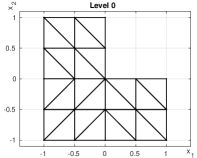
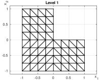
Figure 2. Spatial meshes with uniform refinement strategy: starting mesh and mesh after one refinement step.

As pointed out in Section 3.2.2, spatial meshes with corner-refinements towards the origin are needed to ensure second-order convergence in $L^{2}(\mathrm{D})$ for $\mathbb{P}^{1}$-FEM approximations in $\mathrm{D}$. For a given maximal mesh width $h_{x}>0$, we construct spatial meshes $\mathcal{T}^{N}_{\beta}$ with corner-refinements towards the origin fulfilling the grading condition

(6.12) $$\forall\omega\in\mathcal{T}^{N}_{\beta}\colon\quad h_{x,\omega}\sim\begin{cases}h_{x}^{1/\beta},&\mathrm{dist}(\omega,\boldsymbol{0})=0,\\ h_{x}\cdot\mathrm{dist}(\omega,\boldsymbol{0})^{1-\beta},&0<\mathrm{dist}(\omega,\boldsymbol{0})\leq R,\\ h_{x},&\mathrm{dist}(\omega,\boldsymbol{0})>R,\end{cases}$$

where the mesh grading parameters $\beta\in(0,1]$ and $R>0$ are fixed. Here, $h_{x,\omega}$ is the spatial mesh width of the triangle $\omega\in\mathcal{T}^{N}_{\beta}$, and $\mathrm{dist}(\omega,\boldsymbol{0})$ is the distance of the triangle $\omega\in\mathcal{T}^{N}_{\beta}$ from the origin $\boldsymbol{0}$. To get a sequence of these graded spatial meshes, we halve the maximal mesh width $h_{x}$ and use the newest vertex bisection for the refinement, see Remark 4.4. Figure 3 shows the spatial graded meshes for the first four levels of refinement with mesh grading parameters $\beta=0.6$ and $R=0.25$, which are used in the remainder of this section.

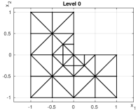
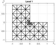
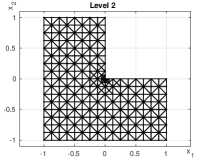
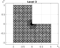
Figure 3. Spatial meshes with corner-refinements towards the origin fulfilling the grading condition (6.12) with parameters $\beta=0.6$ and $R=0.25$.

6.3.2. Spatially Singular Solution

We consider the manufactured solution

(6.13) $$u_{2}(t,x_{1},x_{2})=u_{\mathrm{reg}}(t,x_{1},x_{2})+t\mathrm{e}^{-t}\eta(x_{1},x_{2})\cdot r(x_{1},x_{2})^{2/3}\cdot\sin\left(\frac{2}{3}\left(\arg(x_{1},x_{2})-\frac{\pi}{2}\right)\right)$$

for $(t,x_{1},x_{2})\in\overline{Q}$ with the smooth part

(6.14) $$u_{\mathrm{reg}}(t,x_{1},x_{2})=\frac{1}{100}t\sin(\pi x_{1})\sin(\pi x_{2})\mathrm{e}^{-t\left(x_{1}-\frac{1}{4}\right)^{2}-t\left(x_{2}+\frac{1}{4}\right)^{2}},\quad(t,x_{1},x_{2})\in\overline{Q},$$

where $r(x_{1},x_{2})\in[0,\infty)$ is the radial coordinate, $\arg(x_{1},x_{2})\in(0,2\pi]$ is the angular coordinate, and the cutoff function $\eta\in C^{2}(\mathbb{R}^{2})$ is given by

(6.15) $$\eta(x_{1},x_{2}):=\begin{cases}1,&r(x_{1},x_{2})\leq 1/4,\\ \frac{27}{8}-\frac{135}{4}r(x_{1},x_{2})+180r(x_{1},x_{2})^{2}\\ \quad-440r(x_{1},x_{2})^{3}+480r(x_{1},x_{2})^{4}\\ \quad-192r(x_{1},x_{2})^{5},&1/4<r(x_{1},x_{2})\leq 3/4,\\ 0,&3/4<r(x_{1},x_{2}).\end{cases}$$

Note that the solution $u_{2}$ is smooth in time but has a corner singularity in space, which leads to reduced convergence rates, when the spatial meshes are refined uniformly. Hence, we use the spatial graded meshes as in Figure 3 in order to recover maximal convergence rates. We point out that, in numerical tests not reported here, we have verified that, for a Poisson problem with a solution of regularity as the regularity in space of $u_{2}$ in (6.13), one obtains for the $L^{2}(\mathrm{D})$ error convergence rates $N^{-2/3}\sim h_{x}^{4/3}$ with uniform meshes, and $N^{-1}\sim h_{x}^{2}$ with the considered graded meshes.

For the temporal discretizations, we use $\mathbb{P}^{1}$-FEM approximation on uniformly refined meshes, or $p$-FEM for a fixed number $m=4$ of elements. In connection with the spatial uniform or graded meshes as in Figure 2, Figure 3, respectively, we investigate four possibilities: i) uniform mesh refinement both in space and in time, ii) uniform mesh refinement in space and $p$-FEM in time, iii) graded meshes in space and uniform mesh refinement in time, iv) graded meshes in space and $p$-FEM in time. For all four cases, the numerical results for the space-time Galerkin approximation (6.2) of the solution $u_{2}$ are reported in Figure 4. For a given spatial discretization parameter $N$ and $m=4$ temporal elements, we choose the temporal polynomial degrees $\boldsymbol{p}=(p,p,p,p)$ with $p=\lfloor\frac{\ln N}{2}\rfloor$. This choice of the discretization parameters balances the terms of the error bound (5.11). Hence, the total number of degrees of freedom $MN$ behaves like in (5.12). The numerical results in Figure 4 confirm Remark 5.6.

Figure 4. Numerical results with the space-time Galerkin approximation (6.2) for the 2D example with the singular-in-space solution $u_{2}$ in (6.13), for all combinations of uniform mesh refinement or graded meshes in space (with grading parameter $\beta=0.6$), and $\mathbb{P}^{1}$-FEM with uniform mesh refinement or $p$-FEM in time. For the $p$-FEM in time, for a spatial discretization of parameter $N$, we use a fixed mesh with $m=4$ elements and polynomial degrees $\boldsymbol{p}=(p,p,p,p)$ with $p=\lfloor\frac{\ln N}{2}\rfloor$.

6.3.3. Singular Solution

We consider the singular solution

(6.16) $$u_{3}(t,x_{1},x_{2})=u_{\mathrm{reg}}(t,x_{1},x_{2})\\ +t^{3/5}\mathrm{e}^{-t}\eta(x_{1},x_{2})\cdot r(x_{1},x_{2})^{2/3}\cdot\sin\left(\frac{2}{3}\left(\arg(x_{1},x_{2})-\frac{\pi}{2}\right)\right)$$

for $(t,x_{1},x_{2})\in\overline{Q}$ with the smooth part $u_{\mathrm{reg}}$ in (6.14), the radial coordinate $r(x_{1},x_{2})\in[0,\infty)$, the angular coordinate $\arg(x_{1},x_{2})\in(0,2\pi]$, and the cutoff function $\eta\in C^{2}(\mathbb{R}^{2})$ in (6.15). This solution has a temporal singularity at $t=0$. We observe that the corresponding right-hand side $g_{3}$ does not fulfill the temporal analytic regularity (3.9). On the other hand, solutions with a singular behavior as $u_{3}$ are possible even for sources $g$, which satisfy the condition (3.9). As closed-form representations of such singular solutions do not seem to be available, we perform our numerical tests with the manufactured solution $u_{3}$ in (6.16). Furthermore, the solution $u_{3}$ has the same spatial singularity as $u_{2}$ in (6.13). Thus, in order to get the full convergence rates, we use the graded meshes in Figure 3 for the spatial discretization, and a temporal $hp$-FEM. We investigate four possibilities: i) uniform mesh refinement both in space and in time, ii) uniform mesh refinement in space and $hp$-FEM in time, iii) graded meshes in space and uniform mesh refinement in time, iv) graded meshes in space and $hp$-FEM in time. For all four cases, the numerical results for the space-time Galerkin approximation (6.2) of the solution $u_{3}$ are reported in Figure 5. For a given spatial discretization parameter $N$, we choose the temporal mesh as in (4.1) with grading parameter $\sigma=0.17$, slope parameter $\mu_{\mathrm{hp}}=1.0$, numbers of elements $m_{1}=\lfloor 2.2\cdot\ln N\rfloor$, $m_{2}=1$, and temporal polynomial degrees $\boldsymbol{p}\in\mathbb{N}^{m}$ as in (4.3). This choice of the discretization parameters balances the terms of the error bound (5.9). Hence, the total number of degrees of freedom $MN$ behaves like in (5.10). The numerical results in Figure 5 are in accordance with Theorem 5.5, when the temporal analytic regularity condition (3.9), and hence, the conditions on parameters $\mu_{\mathrm{hp}}$, $m_{2}$, i.e., (5.5), (5.6), are ignored.

Figure 5. Numerical results with the space-time Galerkin approximation (6.2) for the 2D example with the singular solution $u_{3}$ in (6.16), for all combinations of uniform mesh refinement or graded meshes in space (with grading parameter $\beta=0.6$), and $\mathbb{P}^{1}$-FEM with uniform mesh refinement or $hp$-FEM in time. For the $hp$-FEM in time, for a spatial discretization of parameter $N$, we use a geometric temporal mesh with subdivision parameter $\sigma=0.17$, slope parameter $\mu_{\mathrm{hp}}=1.0$, numbers of elements $m_{1}=\lfloor 2.2\cdot\ln N\rfloor$, $m_{2}=1$, and temporal polynomial degrees $\boldsymbol{p}\in\mathbb{N}^{m}$ as in (4.3).

7. Conclusion

Based on a variational space-time formulation of the IBVP (1.1)–(1.3), we analyzed tensorized discretization consisting of an exponentially convergent time-discretization of $hp$-type, combined with a first-order Lagrangian FEM in the spatial domain, with corner-mesh refinement to account for the presence of spatial singularities. Stability of the considered discretization scheme is achieved by Hilbert-transforming the temporal $hp$-trial spaces. Details on the efficient, exponentially accurate, numerical realization of this transformation were presented. Several numerical examples in space dimension $d=2$ in nonconvex polygonal domains confirmed the asymptotic error bounds. In effect, the overall number of degrees of freedom scales essentially as those for one instance of the spatial problem.

The presented proof of time-analyticity via eigenfunction expansions is limited to self-adjoint, elliptic spatial differential operators. Nonselfadjoint spatial operators which are $t$-independent allow similar analytic regularity results via semigroup theory (see, e.g., [28]).

The adopted space-time formulation and its operator perspective and the error analysis extend verbatim to self-adjoint, elliptic spatial operators of positive order. Also, certain nonlinear evolution equations allow for corresponding formulations (see, e.g., [31]). Moreover, transmission problems with piecewise Lipschitz coefficients in the spatial operators can be covered (with the local mesh refinement also at multi-material interface points).

The present error analysis with the same convergence rates is readily extended to a coefficient in the temporal derivative that is time-dependent and analytic in $[0,T]$.

We finally remark that the presently adopted space-time variational formulation will also allow for a posteriori time-discretization error estimation, which is reliable and robust uniformly with respect to $p$. Details shall be developed elsewhere.

Appendix A Some Properties of $H^{1/2}_{0,}(a,b)$

In this appendix, we provide proofs of Lemma 2.1 and Lemma 2.2 of Section 2.1 concerning the Sobolev space $H^{1/2}_{0,}(a,b)$, and state Poincaré and interpolation inequalities in $H^{1/2}_{0,}(a,b)$.

This result of Lemma 2.1 is well-known, but we need to make explicit the dependency of the involved constants on the interval $(a,b)$, which is essential for the derivation of the temporal $hp$-error estimates in Section 5. For simplicity, we restrict to the case of real-valued functions $v\colon\,(a,b)\to\mathbb{R}$. All results and proofs can be generalized straightforwardly to $X$-valued functions $v\colon\,(a,b)\to X$ for a Hilbert space $X$. We introduce the following notation. For the classical Sobolev space

$$H^{1/2}(\mathbb{R})=(H^{1}(\mathbb{R}),L^{2}(\mathbb{R}))_{1/2,2},$$

where $H^{1}(\mathbb{R})$ is equipped with the norm $\|\circ\|_{H^{1}(\mathbb{R})}=(\|\circ\|_{L^{2}(\mathbb{R})}^{2}+\|\partial_{t}\circ\|_{L^{2}(\mathbb{R})}^{2})^{1/2}$, we consider the interpolation norm $\|\circ\|_{H^{1/2}(\mathbb{R})}$ and the Slobodetskii norm

$${\left|\kern-1.07639pt\left|\kern-1.07639pt\left|v\right|\kern-1.07639pt\right|\kern-1.07639pt\right|}_{H^{1/2}(\mathbb{R})}:=\left(\|v\|_{L^{2}(\mathbb{R})}^{2}+|v|_{H^{1/2}(\mathbb{R})}^{2}\right)^{1/2}$$

for $v\in H^{1/2}(\mathbb{R})$, with

$$|v|_{H^{1/2}(\mathbb{R})}:=\left(\int_{-\infty}^{\infty}\int_{-\infty}^{\infty}\frac{|v(s)-v(t)|^{2}}{|s-t|^{2}}\mathrm{d}s\mathrm{d}t\right)^{1/2}.$$

Proof of Lemma 2.1.

The equivalence of norms is proven in, e.g., [24]. We give more details about the norm equivalence constants. For this purpose, we introduce an extension operator and establish bounds on its norm. Define $\mathcal{E}_{1}\colon\,H^{1}_{0,}(a,b)\to H^{1}(\mathbb{R})$,

$$\mathcal{E}_{1}v(t):=\begin{cases}v(t),&t\in[a,b],\\ v(2b-t),&t\in(b,2b-a],\\ 0,&\text{otherwise}\end{cases}$$

for $v\in H^{1}_{0,}(a,b)$. The mapping $\mathcal{E}_{0}\colon\,L^{2}(a,b)\to L^{2}(\mathbb{R})$ is defined for $v\in L^{2}(a,b)$ as

$$\mathcal{E}_{0}v(t):=\begin{cases}v(t),&t\in(a,b),\\ v(2b-t),&t\in(b,2b-a),\\ 0.&\text{otherwise}\end{cases}$$

Evidently, $\mathcal{E}_{1}v=\mathcal{E}_{0}v$ for $v\in H^{1}_{0,}(a,b)$. Next, for $v\in L^{2}(a,b)$,

$${\left\lVert{\mathcal{E}_{0}v}\right\rVert}_{L^{2}(\mathbb{R})}^{2}=\int_{a}^{b}\left\lvert{v(t)}\right\rvert^{2}\mathrm{d}t+\int_{b}^{2b-a}\left\lvert{v(2b-t)}\right\rvert^{2}\mathrm{d}t=2{\left\lVert{v}\right\rVert}_{L^{2}(a,b)}^{2}$$

and, for $v\in H^{1}_{0,}(a,b)$,

$${\left\lVert{\partial_{t}\mathcal{E}_{1}v}\right\rVert}_{L^{2}(\mathbb{R})}^{2}=\int_{a}^{b}\left\lvert{\partial_{t}v(t)}\right\rvert^{2}\mathrm{d}t+\int_{b}^{2b-a}\left\lvert{\partial_{t}v(2b-t)}\right\rvert^{2}\mathrm{d}t=2{\left\lVert{\partial_{t}v}\right\rVert}_{L^{2}(a,b)}^{2}\;.$$

Hence, for $v\in H^{1}_{0,}(a,b)$, it holds true that

$${\left\lVert{\mathcal{E}_{1}v}\right\rVert}_{H^{1}(\mathbb{R})}^{2}=2{\left\lVert{v}\right\rVert}_{H^{1}(a,b)}^{2}\leq 2\left(1+\frac{4(b-a)^{2}}{\pi^{2}}\right){\left\lVert{\partial_{t}v}\right\rVert}_{L^{2}(a,b)}^{2},$$

where the Poincaré inequality (see Lemma A.1 below) is used in the last step. Interpolation yields an operator $\mathcal{E}_{1/2}\colon\,H^{1/2}_{0,}(a,b)\to H^{1/2}(\mathbb{R})$ with $\mathcal{E}_{1/2}v=\mathcal{E}_{0}v$ for $v\in H^{1/2}_{0,}(a,b)$ and

(A.1) $$\forall v\in H^{1/2}_{0,}(a,b):\quad{\left\lVert{\mathcal{E}_{1/2}v}\right\rVert}_{H^{1/2}(\mathbb{R})}^{2}\leq 2\sqrt{1+\frac{4(b-a)^{2}}{\pi^{2}}}{\left\lVert{v}\right\rVert}_{H^{1/2}_{0,}(a,b)}^{2}.$$

Next, we estimate ${\left|\kern-1.07639pt\left|\kern-1.07639pt\left|\mathcal{E}_{1/2}v\right|\kern-1.07639pt\right|\kern-1.07639pt\right|}_{H^{1/2}(\mathbb{R})}$ for $v\in H^{1/2}_{0,}(a,b)$. For this purpose, we compute

$$\left\lvert{\mathcal{E}_{1/2}v}\right\rvert_{H^{1/2}(\mathbb{R})}^{2} =\int_{a}^{\infty}\int_{a}^{\infty}()+2\int_{a}^{\infty}\int_{-\infty}^{a}()+\int_{-\infty}^{a}\int_{-\infty}^{a}()$$

$$=\left\lvert{(\mathcal{E}_{1/2}v)_{|(a,\infty)}}\right\rvert_{H^{1/2}(a,\infty)}^{2}+2\int_{a}^{\infty}\int_{-\infty}^{a}\frac{|\mathcal{E}_{1/2}v(t)|^{2}}{|s-t|^{2}}\mathrm{d}s\mathrm{d}t+0$$

(A.2) $$=\left\lvert{(\mathcal{E}_{1/2}v)_{|(a,\infty)}}\right\rvert_{H^{1/2}(a,\infty)}^{2}+2\int_{a}^{\infty}\frac{\left\lvert{\mathcal{E}_{1/2}v(t)}\right\rvert^{2}}{t-a}\mathrm{d}t$$

for $v\in H^{1/2}_{0,}(a,b)$, where the seminorm $|\circ|_{H^{1/2}(a,\infty)}$ is defined by (2.6) with $b=\infty$. The integral in the bound (A.2) is finite due to $v\in H^{1/2}_{0,}(a,b)$, cf. (2.7). Thus, we get

$${\left|\kern-1.07639pt\left|\kern-1.07639pt\left|\mathcal{E}_{1/2}v\right|\kern-1.07639pt\right|\kern-1.07639pt\right|}_{H^{1/2}(\mathbb{R})}^{2}=2{\left\lVert{v}\right\rVert}_{L^{2}(a,b)}^{2}+\left\lvert{(\mathcal{E}_{1/2}v)_{|(a,\infty)}}\right\rvert_{H^{1/2}(a,\infty)}^{2}+2\int_{a}^{\infty}\frac{\left\lvert{\mathcal{E}_{1/2}v(t)}\right\rvert^{2}}{t-a}\mathrm{d}t\\ =2{\left\lVert{v}\right\rVert}_{L^{2}(a,b)}^{2}+\left\lvert{v}\right\rvert_{H^{1/2}(a,b)}^{2}+2\int_{b}^{\infty}\int_{a}^{b}()+\int_{b}^{\infty}\int_{b}^{\infty}()+2\int_{a}^{\infty}\frac{\left\lvert{\mathcal{E}_{1/2}v(t)}\right\rvert^{2}}{t-a}\mathrm{d}t.$$

The third term on the right side is bounded by

$$2\int_{b}^{\infty}\int_{a}^{b}() =2\int_{b}^{2b-a}\int_{a}^{b}\frac{|v(s)-v(2b-t)|^{2}}{|s-t|^{2}}\mathrm{d}s\mathrm{d}t+2\int_{2b-a}^{\infty}\int_{a}^{b}\frac{|v(s)|^{2}}{|s-t|^{2}}\mathrm{d}s\mathrm{d}t$$

$$=2\int_{a}^{b}\int_{a}^{b}\frac{|v(s)-v(t)|^{2}}{\underbrace{|2b-s-t|^{2}}_{\geq|s-t|^{2}}}\mathrm{d}s\mathrm{d}t+2\int_{a}^{b}\frac{|v(s)|^{2}}{\underbrace{2b-a-s}_{\geq s-a}}\mathrm{d}s$$

$$\leq 2\left\lvert{v}\right\rvert_{H^{1/2}(a,b)}^{2}+2\int_{a}^{b}\frac{|v(s)|^{2}}{s-a}\mathrm{d}s,$$

the fourth term is

$$\int_{b}^{\infty}\int_{b}^{\infty}()=\int_{b}^{2b-a}\int_{b}^{2b-a}()+2\int_{2b-a}^{\infty}\int_{b}^{2b-a}()+\int_{2b-a}^{\infty}\int_{2b-a}^{\infty}()$$

$$=\int_{b}^{2b-a}\int_{b}^{2b-a}\frac{|v(2b-s)-v(2b-t)|^{2}}{|s-t|^{2}}\mathrm{d}s\mathrm{d}t+2\int_{2b-a}^{\infty}\int_{b}^{2b-a}\frac{|v(2b-s)|^{2}}{|s-t|^{2}}\mathrm{d}s\mathrm{d}t+0$$

$$=\left\lvert{v}\right\rvert_{H^{1/2}(a,b)}^{2}+2\int_{b}^{2b-a}\frac{|v(2b-s)|^{2}}{2b-a-s}\mathrm{d}s=\left\lvert{v}\right\rvert_{H^{1/2}(a,b)}^{2}+2\int_{a}^{b}\frac{|v(s)|^{2}}{s-a}\mathrm{d}s,$$

whereas for the fifth term, we have

$$2\int_{a}^{\infty}\frac{\left\lvert{\mathcal{E}_{1/2}v(t)}\right\rvert^{2}}{t-a}\mathrm{d}t =2\int_{a}^{b}\frac{\left\lvert{v(t)}\right\rvert^{2}}{t-a}\mathrm{d}t+2\int_{b}^{2b-a}\frac{\left\lvert{v(2b-t)}\right\rvert^{2}}{t-a}\mathrm{d}t$$

$$=2\int_{a}^{b}\frac{\left\lvert{v(t)}\right\rvert^{2}}{t-a}\mathrm{d}t+2\int_{a}^{b}\frac{\left\lvert{v(t)}\right\rvert^{2}}{\underbrace{2b-a-t}_{\geq t-a}}\mathrm{d}t\leq 4\int_{a}^{b}\frac{\left\lvert{v(t)}\right\rvert^{2}}{t-a}\mathrm{d}t.$$

Using the above estimates gives for all $v\in H^{1/2}_{0,}(a,b)$

$${\left|\kern-1.07639pt\left|\kern-1.07639pt\left|\mathcal{E}_{1/2}v\right|\kern-1.07639pt\right|\kern-1.07639pt\right|}_{H^{1/2}(\mathbb{R})}^{2}\leq 2{\left\lVert{v}\right\rVert}_{L^{2}(a,b)}^{2}+4\left\lvert{v}\right\rvert_{H^{1/2}(a,b)}^{2}+8\int_{a}^{b}\frac{\left\lvert{v(t)}\right\rvert^{2}}{t-a}\mathrm{d}t\leq 8{\left|\kern-1.07639pt\left|\kern-1.07639pt\left|v\right|\kern-1.07639pt\right|\kern-1.07639pt\right|}_{H^{1/2}_{0,}(a,b)}^{2}\;.$$

With these properties, we have for all $v\in H^{1/2}_{0,}(a,b)$ the lower bound in the norm equivalence:

$${\left\lVert{v}\right\rVert}_{H^{1/2}_{0,}(a,b)}\leq{\left\lVert{\mathcal{E}_{1/2}v}\right\rVert}_{H^{1/2}(\mathbb{R})}\leq\frac{1}{C_{\mathbb{R},1}}{\left|\kern-1.07639pt\left|\kern-1.07639pt\left|\mathcal{E}_{1/2}v\right|\kern-1.07639pt\right|\kern-1.07639pt\right|}_{H^{1/2}(\mathbb{R})}\leq\frac{2\sqrt{2}}{C_{\mathbb{R},1}}{\left|\kern-1.07639pt\left|\kern-1.07639pt\left|v\right|\kern-1.07639pt\right|\kern-1.07639pt\right|}_{H^{1/2}_{0,}(a,b)}\;.$$

Here, the first inequality is proven by interpolation, the second estimate follows from

(A.3) $$\forall z\in H^{1/2}(\mathbb{R}):\quad C_{\mathbb{R},1}{\left\lVert{z}\right\rVert}_{H^{1/2}(\mathbb{R})}\leq{\left|\kern-1.07639pt\left|\kern-1.07639pt\left|z\right|\kern-1.07639pt\right|\kern-1.07639pt\right|}_{H^{1/2}(\mathbb{R})}\leq C_{\mathbb{R},2}{\left\lVert{z}\right\rVert}_{H^{1/2}(\mathbb{R})}$$

with constants $C_{\mathbb{R},1}$, $C_{\mathbb{R},2}>0$, see [24, Theorem B.7] and [12, Lemma 4.1].

For the upper bound, relations (A.2), (A.3) and (A.1) yield

$${\left|\kern-1.07639pt\left|\kern-1.07639pt\left|v\right|\kern-1.07639pt\right|\kern-1.07639pt\right|}_{H^{1/2}_{0,}(a,b)}^{2} \leq{\left\lVert{\mathcal{E}_{1/2}v}\right\rVert}_{L^{2}(\mathbb{R})}^{2}+\left\lvert{(\mathcal{E}_{1/2}v)_{|(a,\infty)}}\right\rvert_{H^{1/2}(a,\infty)}^{2}+\int_{a}^{\infty}\frac{\left\lvert{\mathcal{E}_{1/2}v(t)}\right\rvert^{2}}{t-a}\mathrm{d}t$$

$$={\left\lVert{\mathcal{E}_{1/2}v}\right\rVert}_{L^{2}(\mathbb{R})}^{2}+\frac{1}{2}\left\lvert{(\mathcal{E}_{1/2}v)_{|(a,\infty)}}\right\rvert_{H^{1/2}(a,\infty)}^{2}+\frac{1}{2}\left\lvert{\mathcal{E}_{1/2}v}\right\rvert_{H^{1/2}(\mathbb{R})}^{2}$$

$$\leq{\left|\kern-1.07639pt\left|\kern-1.07639pt\left|\mathcal{E}_{1/2}v\right|\kern-1.07639pt\right|\kern-1.07639pt\right|}_{H^{1/2}(\mathbb{R})}^{2}$$

$$\leq(C_{\mathbb{R},2})^{2}{\left\lVert{\mathcal{E}_{1/2}v}\right\rVert}_{H^{1/2}(\mathbb{R})}^{2}\leq(C_{\mathbb{R},2})^{2}2\sqrt{1+\frac{4(b-a)^{2}}{\pi^{2}}}{\left\lVert{v}\right\rVert}_{H^{1/2}_{0,}(a,b)}^{2},$$

i.e., the assertion is proven. ∎

The following proof of Lemma 2.2 restricts the argument of [13] to our particular case.

Proof of Lemma 2.2.

Let $v\in H^{1/2}(a,b)$ and $\tau\in(a,b$) be given. Then, we split the integral in the definition (2.6) as follows:

$$|v|_{H^{1/2}(a,b)}^{2} =\int_{a}^{\tau}\int_{a}^{b}\Big{(}\cdots\Big{)}\mathrm{d}s\mathrm{d}t+\int_{\tau}^{b}\int_{a}^{b}\Big{(}\cdots\Big{)}\mathrm{d}s\mathrm{d}t$$

$$=\int_{a}^{\tau}\int_{a}^{\tau}\Big{(}\cdots\Big{)}\mathrm{d}s\mathrm{d}t+2\int_{a}^{\tau}\int_{\tau}^{b}\Big{(}\cdots\Big{)}\mathrm{d}s\mathrm{d}t+\int_{\tau}^{b}\int_{\tau}^{b}\Big{(}\cdots\Big{)}\mathrm{d}s\mathrm{d}t$$

$$=|v|_{H^{1/2}(a,\tau)}^{2}+2\int_{a}^{\tau}\int_{\tau}^{b}\Big{(}\cdots\Big{)}\mathrm{d}s\mathrm{d}t+|v|_{H^{1/2}(\tau,b)}^{2}.$$

For the integral on the right side, we get

$$2\int_{a}^{\tau}\int_{\tau}^{b}\frac{|v(s)-v(t)|^{2}}{|s-t|^{2}}\mathrm{d}s\mathrm{d}t \leq 4\int_{a}^{\tau}\int_{\tau}^{b}\frac{|v(s)|^{2}}{|s-t|^{2}}\mathrm{d}s\mathrm{d}t+4\int_{a}^{\tau}\int_{\tau}^{b}\frac{|v(t)|^{2}}{|s-t|^{2}}\mathrm{d}s\mathrm{d}t$$

$$=4\int_{\tau}^{b}|v(s)|^{2}[(s-\tau)^{-1}-(s-a)^{-1}]\mathrm{d}s$$

$$\quad+4\int_{a}^{\tau}|v(t)|^{2}[(\tau-t)^{-1}-(b-t)^{-1}]\mathrm{d}t$$

$$\leq 4\int_{\tau}^{b}\frac{|v(s)|^{2}}{s-\tau}\mathrm{d}s+4\int_{a}^{\tau}\frac{|v(t)|^{2}}{\tau-t}\mathrm{d}t.$$

Thus, the assertion follows. ∎

Lemma A.1.

For $a,b\in\mathbb{R}$, $a<b$, the Poincaré inequalities

$$\forall v\in H^{1/2}_{0,}(a,b):\quad \|v\|_{L^{2}(a,b)}\leq\sqrt{\frac{2(b-a)}{\pi}}\|v\|_{H^{1/2}_{0,}(a,b)},$$

$$\forall v\in H^{1}_{0,}(a,b):\quad \|v\|_{H^{1/2}_{0,}(a,b)}\leq\sqrt{\frac{2(b-a)}{\pi}}\|\partial_{t}v\|_{L^{2}(a,b)},$$

$$\forall v\in H^{1}_{0,}(a,b):\quad \|v\|_{L^{2}(a,b)}\leq\frac{2(b-a)}{\pi}\|\partial_{t}v\|_{L^{2}(a,b)}$$

hold true, where the constants are sharp.

Proof.

By interpolation, we have the Fourier series representations

(A.4) $$\|v\|_{L^{2}(a,b)}^{2}=\sum_{k=0}^{\infty}|v_{k}|^{2},\quad\|v\|_{H^{1/2}_{0,}(a,b)}^{2}=\sum_{k=0}^{\infty}\sqrt{\lambda_{k}}|v_{k}|^{2},\quad\|\partial_{t}v\|_{L^{2}(a,b)}^{2}=\sum_{k=0}^{\infty}\lambda_{k}|v_{k}|^{2}$$

with coefficients $v_{k}$ as in (2.2) and eigenvalues $\lambda_{k}=\frac{\pi^{2}(2k+1)^{2}}{4(b-a)^{2}}$ of the eigenvalue problem (2.3). Hence, all Poincaré inequalities follow from these representations. The constants are sharp since for $v$ with $v_{0}\neq 0$ and $v_{k}=0$ for $k\in\mathbb{N}$, equality holds true. ∎

Lemma A.2.

For $a,b\in\mathbb{R}$ with $a<b$, the interpolation estimate

$$\forall v\in H^{1}_{0,}(a,b):\,\|v\|_{H^{1/2}_{0,}(a,b)}\leq\sqrt{\|v\|_{L^{2}(a,b)}\|\partial_{t}v\|_{L^{2}(a,b)}}$$

holds true, where $\|\circ\|_{H^{1/2}_{0,}(a,b)}$ denotes the interpolation norm (2.1).

Proof.

Using the Cauchy–Schwarz inequality, the assertion follows immediately from the Fourier representations (A.4). ∎

Appendix B Proof of Lemma 3.6

Let $b\in(0,T]$ be fixed. According to (3.11) for $l=0$, the estimate

$$\forall t>0\colon{\left\lVert{E(t)}\right\rVert}_{\mathcal{L}(X_{\varepsilon},X_{2})}^{2}\leq\frac{1}{\sqrt{2\pi}}\left(\frac{1}{2}\right)^{2-\varepsilon}\Gamma(3-\varepsilon)t^{-2+\varepsilon}.$$

holds true. The logarithmic convexity of the gamma function gives $\Gamma(3-\varepsilon)=\Gamma\left(2\varepsilon+3(1-\varepsilon)\right)\leq\Gamma(2)^{\varepsilon}\Gamma(3)^{1-\varepsilon}=2^{1-\varepsilon}$ and we obtain

(B.1) $$\forall t>0\colon{\left\lVert{E(t)}\right\rVert}_{\mathcal{L}(X_{\varepsilon},X_{2})}\leq\sqrt{\frac{1}{\sqrt{2\pi}}\left(\frac{1}{2}\right)t^{-2+\varepsilon}}=\frac{1}{\sqrt[4]{8\pi}}\,t^{-1+\varepsilon/2}.$$

The solution $u$ admits the representation

(B.2) $$u(t)=\int_{0}^{t}E(\tau)g(t-\tau)\mathrm{d}\tau,\quad 0\leq t\leq b,$$

see (3.8), and for $t\in[0,b]$, it follows that

$${\left\lVert{u(t)}\right\rVert}_{X_{2}} \leq\int_{0}^{t}{\left\lVert{E(\tau)g(t-\tau)}\right\rVert}_{X_{2}}\mathrm{d}\tau\leq\int_{0}^{t}{\left\lVert{E(\tau)}\right\rVert}_{\mathcal{L}(X_{\varepsilon},X_{2})}{\left\lVert{g(t-\tau)}\right\rVert}_{X_{\varepsilon}}\mathrm{d}\tau$$

$$\leq\frac{1}{\sqrt[4]{8\pi}}C_{g}\int_{0}^{t}\tau^{-1+\varepsilon/2}\mathrm{d}\tau=\frac{1}{\sqrt[4]{8\pi}}C_{g}\,\frac{2}{\varepsilon}\,t^{\varepsilon/2}=\sqrt[4]{\frac{2}{\pi}}\,C_{g}\,\frac{1}{\varepsilon}\,t^{\varepsilon/2}.$$

We estimate the three terms of ${\left|\kern-1.07639pt\left|\kern-1.07639pt\left|u\right|\kern-1.07639pt\right|\kern-1.07639pt\right|}_{H^{1/2}_{0,}((0,b);X_{2})}$ expressed as in (2.7).

First term: From the previous bound for ${\left\lVert{u(t)}\right\rVert}_{X_{2}}$, we derive

$$\|u\|_{L^{2}((0,b);X_{2})}^{2}=\int_{0}^{b}{\left\lVert{u(t)}\right\rVert}_{X_{2}}^{2}\mathrm{d}t\leq\sqrt{\frac{2}{\pi}}\,C_{g}^{2}\,\frac{1}{\varepsilon^{2}}\int_{0}^{b}t^{\varepsilon}\mathrm{d}t=\sqrt{\frac{2}{\pi}}\,C_{g}^{2}\,\frac{1}{\varepsilon^{2}(1+\varepsilon)}\,b^{1+\varepsilon}.$$

Third term: Similarly, we obtain

$$\int_{0}^{b}\frac{{\left\lVert{u(t)}\right\rVert}_{X_{2}}^{2}}{t}\mathrm{d}t\leq\sqrt{\frac{2}{\pi}}\,C_{g}^{2}\,\frac{1}{\varepsilon^{2}}\int_{0}^{b}t^{\varepsilon-1}\mathrm{d}t=\sqrt{\frac{2}{\pi}}\,C_{g}^{2}\,\frac{1}{\varepsilon^{3}}\,b^{\varepsilon}.$$

Second term: Recalling (2.6), we need to estimate $\int_{0}^{b}\int_{0}^{b}\frac{\|u(s)-u(t)\|_{X_{2}}^{2}}{|s-t|^{2}}\mathrm{d}s\mathrm{d}t$.
For $b\geq s\geq t\geq 0$, we have

$${\left\lVert{u(s)-u(t)}\right\rVert}_{X_{2}}\stackrel{{\scriptstyle\eqref{eq:repr}}}{{=}}{\left\lVert{\int_{0}^{s}E(\tau)g(s-\tau)\mathrm{d}\tau-\int_{0}^{t}E(\tau)g(t-\tau)\mathrm{d}\tau}\right\rVert}_{X_{2}}$$

$$\qquad={\left\lVert{\int_{t}^{s}E(\tau)g(s-\tau)\mathrm{d}\tau+\int_{0}^{t}E(\tau)g(s-\tau)\mathrm{d}\tau-\int_{0}^{t}E(\tau)g(t-\tau)\mathrm{d}\tau}\right\rVert}_{X_{2}}$$

$$\qquad\leq{\left\lVert{\int_{t}^{s}E(\tau)g(s-\tau)\mathrm{d}\tau}\right\rVert}_{X_{2}}+{\left\lVert{\int_{0}^{t}E(\tau)[g(s-\tau)-g(t-\tau)]\mathrm{d}\tau}\right\rVert}_{X_{2}}$$

$$\qquad\leq\int_{t}^{s}{\left\lVert{E(\tau)}\right\rVert}_{\mathcal{L}(X_{\varepsilon},X_{2})}{\left\lVert{g(s-\tau)}\right\rVert}_{X_{\varepsilon}}\mathrm{d}\tau$$

$$\qquad\quad+\int_{0}^{t}{\left\lVert{E(\tau)}\right\rVert}_{\mathcal{L}(X_{\varepsilon},X_{2})}{\left\lVert{g(s-\tau)-g(t-\tau)}\right\rVert}_{X_{\varepsilon}}\mathrm{d}\tau$$

$$\qquad\stackrel{{\scriptstyle\eqref{eq:Tt}}}{{\leq}}\frac{1}{\sqrt[4]{8\pi}}\left(\int_{t}^{s}\tau^{-1+\varepsilon/2}{\left\lVert{g(s-\tau)}\right\rVert}_{X_{\varepsilon}}\mathrm{d}\tau+\int_{0}^{t}\tau^{-1+\varepsilon/2}{\left\lVert{\int_{t-\tau}^{s-\tau}g^{\prime}(r)dr}\right\rVert}_{X_{\varepsilon}}\mathrm{d}\tau\right)$$

$$\qquad\stackrel{{\scriptstyle\eqref{eq:boundg}}}{{\leq}}\frac{1}{\sqrt[4]{8\pi}}\,C_{g}\,\frac{2}{\varepsilon}\,\left((s^{\varepsilon/2}-t^{\varepsilon/2})+t^{\varepsilon/2}\,(s-t)\right).$$

Analogously, for $b\geq t\geq s\geq 0$, the estimate

$${\left\lVert{u(s)-u(t)}\right\rVert}_{X_{2}}\leq\frac{1}{\sqrt[4]{8\pi}}\,C_{g}\,\frac{2}{\varepsilon}\,\left((t^{\varepsilon/2}-s^{\varepsilon/2})+s^{\varepsilon/2}\,(t-s)\right)$$

holds true. We conclude that

$$\int_{0}^{b}\int_{0}^{b} \frac{\|u(s)-u(t)\|_{X_{2}}^{2}}{|s-t|^{2}}\mathrm{d}s\mathrm{d}t$$

$$=\int_{0}^{b}\int_{0}^{t}\frac{\|u(s)-u(t)\|_{X_{2}}^{2}}{|s-t|^{2}}\mathrm{d}s\mathrm{d}t+\int_{0}^{b}\int_{0}^{s}\frac{\|u(s)-u(t)\|_{X_{2}}^{2}}{|s-t|^{2}}\mathrm{d}t\mathrm{d}s$$

$$\leq\frac{1}{\sqrt{8\pi}}\,C_{g}^{2}\,\frac{16}{\varepsilon^{2}}\int_{0}^{b}\int_{0}^{s}\left(\frac{(s^{\varepsilon/2}-t^{\varepsilon/2})^{2}}{(s-t)^{2}}+t^{\varepsilon}\right)\mathrm{d}t\mathrm{d}s$$

$$=\sqrt{\frac{32}{\pi}}\,\frac{1}{\varepsilon^{2}}\,C_{g}^{2}\left(\int_{0}^{b}s^{-1+\varepsilon}\int_{0}^{1}\frac{(1-r^{\varepsilon/2})^{2}}{(1-r)^{2}}\mathrm{d}r\mathrm{d}s+\frac{b^{\varepsilon+2}}{(\varepsilon+1)(\varepsilon+2)}\right)$$

$$\stackrel{{\scriptstyle\text{$\varepsilon/2\leq 1$}}}{{\leq}}\sqrt{\frac{32}{\pi}}\,\frac{1}{\varepsilon^{2}}\,C_{g}^{2}\left(\int_{0}^{b}s^{-1+\varepsilon}\int_{0}^{1}\frac{(1-r^{\varepsilon/2})^{2}}{(1-r^{\varepsilon/2})^{2}}\mathrm{d}r\mathrm{d}s+\frac{b^{\varepsilon+2}}{(\varepsilon+1)(\varepsilon+2)}\right)$$

$$=\sqrt{\frac{32}{\pi}}\,\frac{1}{\varepsilon^{2}}\,C_{g}^{2}\left(\frac{b^{\varepsilon}}{\varepsilon}+\frac{b^{\varepsilon+2}}{(\varepsilon+1)(\varepsilon+2)}\right).$$

Conclusion of the proof: By combining the bounds of the three terms, we arrive at the a priori estimate

$${\left|\kern-1.07639pt\left|\kern-1.07639pt\left|u\right|\kern-1.07639pt\right|\kern-1.07639pt\right|}_{H^{1/2}_{0,}((0,b);X_{2})}\leq\sqrt[4]{\frac{2}{\pi}}\,\frac{1}{\varepsilon}\,b^{\varepsilon/2}\left(\frac{b}{1+\varepsilon}+\frac{3}{\varepsilon}+\frac{4b^{2}}{(\varepsilon+1)(\varepsilon+2)}\right)^{1/2}C_{g}\;,$$

which gives the assertion.

Appendix C Proof of Lemma 5.2

This proof is a slight modification of the proof of [11, Lemma 3.4]. We use Stirling’s inequalities

(C.1) $$\forall x>0:\quad\sqrt{2\pi}x^{x-1/2}\mathrm{e}^{-x}\leq\Gamma(x)\leq\sqrt{2\pi}x^{x-1/2}\mathrm{e}^{-x}\mathrm{e}^{\frac{1}{12x}}.$$

For $j\geq 1$, (C.1) yields

$$\frac{\Gamma(\lfloor\mu j\rfloor-j+1)}{\Gamma(\lfloor\mu j\rfloor+j+1)}\leq\frac{\Gamma(\mu j-j+1)}{\Gamma(\mu j+j)}\\ \leq\frac{\sqrt{2\pi}(\overbrace{\mu j-j+1}^{\leq\mu j\text{ as }j\geq 1})^{\overbrace{\mu j-j+1/2}^{\geq 0\text{ as }\mu\geq 1}}\mathrm{e}^{-(\mu j-j+1)}\overbrace{\mathrm{e}^{1/(12(\mu j-j+1))}}^{\leq 2}}{\sqrt{2\pi}(\underbrace{\mu j+j}_{\geq\mu j})^{\mu j+j-1/2}\mathrm{e}^{-(\mu j+j)}}\leq\frac{2\mu j}{\mathrm{e}}\left(\frac{\mathrm{e}}{\mu j}\right)^{2j}$$

and

$$\Gamma(j+3)^{2}=(\underbrace{j+2}_{\leq 3j})^{2}(\underbrace{j+1}_{\leq 2j})^{2}j^{2}\Gamma(j)^{2}\leq j^{6}\cdot 72\pi j^{2j-1}\mathrm{e}^{-2j}\underbrace{\mathrm{e}^{\frac{1}{6j}}}_{<2}\leq 144\pi j^{5}j^{2j}\mathrm{e}^{-2j}.$$

Thus, we have

$$\forall j\in\mathbb{N}:\quad\alpha^{2j}\frac{\Gamma(\lfloor\mu j\rfloor-j+1)}{\Gamma(\lfloor\mu j\rfloor+j+1)}\Gamma(j+3)^{2}\leq\frac{288\pi\mu}{\mathrm{e}}j^{6}\left(\frac{\alpha}{\mu}\right)^{2j}.$$

Hence, we conclude that

$$\sum_{j=0}^{m}\alpha^{2j}\frac{\Gamma(\lfloor\mu j\rfloor-j+1)}{\Gamma(\lfloor\mu j\rfloor+j+1)}\Gamma(j+3)^{2}=4+\sum_{j=1}^{m}\alpha^{2j}\frac{\Gamma(\lfloor\mu j\rfloor-j+1)}{\Gamma(\lfloor\mu j\rfloor+j+1)}\Gamma(j+3)^{2}\\ \leq 4+\frac{288\pi\mu}{\mathrm{e}}\sum_{j=1}^{\infty}j^{6}\left(\frac{\alpha}{\mu}\right)^{2j}<\infty,$$

since the ratio test gives

$$\lim_{j\to\infty}\frac{(j+1)^{6}\left(\frac{\alpha}{\mu}\right)^{2(j+1)}}{j^{6}\left(\frac{\alpha}{\mu}\right)^{2j}}=\left(\frac{\alpha}{\mu}\right)^{2}<1,$$

i.e., the assertion is proven.

References

• [1] James H. Adler and Victor Nistor, Graded mesh approximation in weighted Sobolev spaces and elliptic equations in 2D, Math. Comp. 84 (2015), no. 295, 2191–2220. MR 3356024
• [2] Bernd Ammann and Victor Nistor, Weighted Sobolev spaces and regularity for polyhedral domains, Comput. Methods Appl. Mech. Engrg. 196 (2007), no. 37-40, 3650–3659. MR 2339991
• [3] Roman Andreev, Stability of sparse space-time finite element discretizations of linear parabolic evolution equations, IMA J. Numer. Anal. 33 (2013), no. 1, 242–260. MR 3020957
• [4] Thomas Apel, Anisotropic finite elements: local estimates and applications, Advances in Numerical Mathematics, B. G. Teubner, Stuttgart, 1999. MR 1716824
• [5] I. Babuška, R. B. Kellogg, and J. Pitkäranta, Direct and inverse error estimates for finite elements with mesh refinements, Numer. Math. 33 (1979), no. 4, 447–471. MR 553353
• [6] Constantin Bacuta, Victor Nistor, and Ludmil T. Zikatanov, Improving the rate of convergence of high-order finite elements on polyhedra. I. A priori estimates, Numer. Funct. Anal. Optim. 26 (2005), no. 6, 613–639. MR 2187917
• [7] by same author, Improving the rate of convergence of high-order finite elements on polyhedra. II. Mesh refinements and interpolation, Numer. Funct. Anal. Optim. 28 (2007), no. 7-8, 775–824. MR 2347683
• [8] Constantin Băcuţă, Hengguang Li, and Victor Nistor, Differential operators on domains with conical points: precise uniform regularity estimates, Rev. Roumaine Math. Pures Appl. 62 (2017), no. 3, 383–411. MR 3711082
• [9] Andrea Cangiani, Zhaonan Dong, and Emmanuil H. Georgoulis, $hp$-version space-time discontinuous Galerkin methods for parabolic problems on prismatic meshes, SIAM J. Sci. Comput. 39 (2017), no. 4, A1251–A1279. MR 3672375
• [10] Philip J. Davis, Interpolation and approximation, Dover Publications, Inc., New York, 1975. MR 0380189
• [11] Denis Devaud, Petrov-Galerkin space-time $hp$-approximation of parabolic equations in $H^{1/2}$, IMA J. Numer. Anal. 40 (2020), no. 4, 2717–2745. MR 4167060
• [12] G. I. Eskin, Boundary value problems for elliptic pseudodifferential equations, Translations of Mathematical Monographs, vol. 52, American Mathematical Society, Providence, R.I., 1981. MR 623608
• [13] Birgit Faermann, Localization of the Aronszajn-Slobodeckij norm and application to adaptive boundary element methods. I. The two-dimensional case, IMA J. Numer. Anal. 20 (2000), no. 2, 203–234. MR 1752263
• [14] Thomas Führer and Michael Karkulik, Space-time least-squares finite elements for parabolic equations, Comput. Math. Appl. 92 (2021), 27–36. MR 4242919
• [15] Gregor Gantner and Rob Stevenson, Further results on a space-time FOSLS formulation of parabolic PDEs, ESAIM Math. Model. Numer. Anal. 55 (2021), no. 1, 283–299. MR 4216839
• [16] Fernando D. Gaspoz and Pedro Morin, Approximation classes for adaptive higher order finite element approximation, Math. Comp. 83 (2014), no. 289, 2127–2160. MR 3223327
• [17] Walter Gautschi, Numerical integration over the square in the presence of algebraic/logarithmic singularities with an application to aerodynamics, Numer. Algorithms 61 (2012), no. 2, 275–290.
• [18] Michael Griebel, Daniel Oeltz, and Panayot Vassilevski, Space-time approximation with sparse grids, SIAM J. Sci. Comput. 28 (2006), no. 2, 701–727. MR 2231727
• [19] Angela Kunoth and Christoph Schwab, Analytic regularity and GPC approximation for control problems constrained by linear parametric elliptic and parabolic PDEs, SIAM J. Control Optim. 51 (2013), no. 3, 2442–2471. MR 3064588
• [20] Ulrich Langer, Stephen E. Moore, and Martin Neumüller, Space-time isogeometric analysis of parabolic evolution problems, Comput. Methods Appl. Mech. Engrg. 306 (2016), 342–363. MR 3502571
• [21] Ulrich Langer and Marco Zank, Efficient direct space-time finite element solvers for parabolic initial-boundary value problems in anisotropic Sobolev spaces, SIAM J. Sci. Comput. 43 (2021), no. 4, A2714–A2736. MR 4295048
• [22] Hengguang Li, Anna Mazzucato, and Victor Nistor, Analysis of the finite element method for transmission/mixed boundary value problems on general polygonal domains, Electron. Trans. Numer. Anal. 37 (2010), 41–69. MR 2777235
• [23] Vladimir Maz’ya and Jürgen Rossmann, Elliptic equations in polyhedral domains, Mathematical Surveys and Monographs, vol. 162, American Mathematical Society, Providence, RI, 2010. MR 2641539
• [24] William McLean, Strongly elliptic systems and boundary integral equations, Cambridge University Press, Cambridge, 2000. MR 1742312
• [25] Monica Montardini, Matteo Negri, Giancarlo Sangalli, and Mattia Tani, Space-time least-squares isogeometric method and efficient solver for parabolic problems, Math. Comp. 89 (2020), no. 323, 1193–1227. MR 4063316
• [26] Amnon Pazy, Semigroups of linear operators and applications to partial differential equations, Applied Mathematical Sciences, vol. 44, Springer-Verlag, New York, 1983. MR 710486
• [27] Dominik Schötzau and Christoph Schwab, Time Discretization of Parabolic Problems by the $hp$-Version of the Discontinuous Galerkin Finite Element Method, SIAM J. Numer. Anal. 38 (2000), no. 3, 837–875.
• [28] Dominik Schötzau and Christoph Schwab, $hp$-discontinuous Galerkin time-stepping for parabolic problems, C. R. Acad. Sci. Paris Sér. I Math. 333 (2001), no. 12, 1121–1126. MR 1881245
• [29] Christoph Schwab, $p$- and $hp$-finite element methods, Numerical Mathematics and Scientific Computation, The Clarendon Press, Oxford University Press, New York, 1998, Theory and applications in solid and fluid mechanics. MR 1695813
• [30] Christoph Schwab and Rob Stevenson, Space-time adaptive wavelet methods for parabolic evolution problems, Math. Comp. 78 (2009), no. 267, 1293–1318. MR 2501051
• [31] by same author, Fractional space-time variational formulations of (Navier-) Stokes equations, SIAM J. Math. Anal. 49 (2017), no. 4, 2442–2467. MR 3668596
• [32] Olaf Steinbach, Space-time finite element methods for parabolic problems, Comput. Methods Appl. Math. 15 (2015), no. 4, 551–566. MR 3403450
• [33] Olaf Steinbach and Agnese Missoni, A note on a modified Hilbert transform, Applicable Analysis (2022), 1–8.
• [34] Olaf Steinbach and Marco Zank, Coercive space-time finite element methods for initial boundary value problems, Electron. Trans. Numer. Anal. 52 (2020), 154–194. MR 4102914
• [35] by same author, A note on the efficient evaluation of a modified Hilbert transformation, J. Numer. Math. 29 (2021), no. 1, 47–61. MR 4230416
• [36] Rob Stevenson and Jan Westerdiep, Stability of Galerkin discretizations of a mixed space-time variational formulation of parabolic evolution equations, IMA J. Numer. Anal. 41 (2021), no. 1, 28–47. MR 4205051
• [37] Vidar Thomée, Galerkin finite element methods for parabolic problems, second ed., Springer Series in Computational Mathematics, vol. 25, Springer-Verlag, Berlin, 2006. MR 2249024
• [38] Hans Triebel, Interpolation theory, function spaces, differential operators, second ed., Johann Ambrosius Barth, Heidelberg, 1995. MR 1328645
• [39] Marco Zank, An exact realization of a modified Hilbert transformation for space-time methods for parabolic evolution equations, Comput. Methods Appl. Math. 21 (2021), no. 2, 479–496. MR 4235810