An Optimal Transport Formulation of Bayes’ Law
for Nonlinear Filtering Algorithms

Abstract

This paper presents a variational representation of the Bayes’ law using optimal transportation theory. The variational representation is in terms of the optimal transportation between the joint distribution of the (state, observation) and their independent coupling. By imposing certain structure on the transport map, the solution to the variational problem is used to construct a Brenier-type map that transports the prior distribution to the posterior distribution for any value of the observation signal. The new formulation is used to derive the optimal transport form of the Ensemble Kalman filter (EnKF) for the discrete-time filtering problem and propose a novel extension of EnKF to the non-Gaussian setting utilizing input convex neural networks. Finally, the proposed methodology is used to derive the optimal transport form of the feedback particle filler (FPF) in the continuous-time limit, which constitutes its first variational construction without explicitly using the nonlinear filtering equation or Bayes’ law.

I Introduction

Nonlinear filtering is the problem of computing the conditional distribution of the state of a stochastic dynamical system given historical noisy observations. The critical step in any nonlinear filtering algorithm is the implementation of Bayes’ law in order to update the conditional distribution of the state as the new observations arrive. Bayes’ law gives the conditional distribution of the state $X$ given observations $Y$ according to

$$P_{X|Y}(x|y)=\frac{P_{X}(x)P_{Y|X}(y|x)}{P_{Y}(y)}$$ (1)

where $P_{X}$ is the prior distribution assumed on $X$, $P_{Y|X}$ is the likelihood distribution of observations conditioned on the state $X$, and $P_{Y}(y)=\int P_{Y|X}(y|x)P_{X}(x)\,\mathrm{d}x$ is the marginal distribution of $Y$. Nonlinear filtering is also accompanied with an update step according to the dynamics of the system. This step is straightforward using the dynamic model directly. Therefore, the focus of this paper is on the Bayesian update step.

Numerical implementations of Bayes’ law often require a discretization (finite-dimensional approximation) of the prior and posterior distributions. An exact computation is not possible except in a few special cases, such as the class of Gaussian distributions or in the finite-state space setting. This motivates Monte-Carlo or particle-based approaches where the posterior distribution is approximated with an empirical distribution of samples. To this end, the main task of a particle-based algorithm is to transform a set of particles that represent samples from the prior distribution to particles that represent the posterior distribution. Simply put, the problem can be stated as:

given: $$~{}\{X^{1}_{0},\ldots,X^{N}_{0}\}\sim P_{X}$$

generate: $$~{}\{X^{1}_{1},\ldots,X^{N}_{1}\}\sim P_{X|Y}$$

A vanilla importance sampling and resampling particle filter carries out this task by first forming a weighted empirical distribution and then resampling from the weighted distribution [12]:

$$X^{i}_{1}\sim\sum_{j=1}^{N}w_{j}\delta_{X^{j}_{0}},\quad w_{j}=\frac{P_{Y|X}(y|X^{j}_{0})}{\sum_{k=1}^{N}P_{Y|X}(y|X^{k}_{0})}.$$

Although computationally efficient, this approach performs poorly in high-dimensional problems due to weight degeneracy issues [27, 4, 2]. In particular, for a Gaussian prior and identity observation model, the mean-squared error scales with $\frac{C^{d}}{N}$ where $d$ is the dimension of the state and $C$ is a positive constant [36]. This means that in order to keep the same error, the number of particles $N$ should scale exponentially with the dimension $d$.

These issues motivated recent efforts in the nonlinear filtering literature to develop numerical algorithms based on a controlled system of interacting particles to approximate the posterior distribution [40, 39, 9, 28, 31, 3, 10, 11]. A prominent idea is to view the problem of transforming samples from the prior to the posterior from the lens of optimal transportation theory  [29, 30, 36, 8, 35, 37], which has also become popular in the Bayesian inference literature [13, 23, 24, 18, 34, 20, 33]. Broadly speaking, the aim of the above methods is to find a transport map (be it stochastic or deterministic) that transforms the prior distribution to the posterior distribution while minimizing a certain cost.

The present paper builds on the aforementioned transport-based works and is closely related to the optimal transport formulation of the Ensemble Kalman filter (EnKF) and feedback particle filter (FPF) [36, 37] with a slight, but crucial, difference in the formulation: Prior works are based on optimal transportation from the prior $P_{X}$ to the posterior $P_{X|Y}$, which is undesirable as the posterior distribution is not available and depends on the observation $Y$. Instead, the new formulation involves the optimal transportation between the independent coupling $P_{X}\otimes P_{Y}$ and the joint distribution $P_{XY}$ which is readily available in a filtering problem. By imposing a block triangular structure $(x,y)\mapsto S(x,y)=(T(x,y),y)$ on the transport map $S$, the component $T(x,y)$ automatically serves as a transport map between the prior and posterior distributions for any realization of the observation $Y=y$. Such triangular representations of the transport map have also appeared in [13, 34, 20, 26, 32]. With the map $T$ at hand, one can generate samples from the posterior distribution $P_{X|Y=y}$ according to

$$X^{i}_{1}=T(X^{i}_{0},y),\quad\text{for}\quad i=1,\ldots,N.$$

This slight difference in the formulation of the transport problem has several implications which constitute the contributions of the paper:

• A variational formulation of Bayes’ law is introduced that is based on the Kantorovich dual formulation of a optimal transportation problem between $P_{X}\otimes P_{Y}$ and $P_{XY}$. The solution to this problem is a Brenier-type map (the map $T$ above) that characterizes the posterior.

• The variational formulation is cast as a stochastic optimization problem that requires pairs of samples $\{(X^{i},Y^{i})\}_{i=1}^{N}$ from the joint distribution $P_{XY}$. The pair of samples can be generated using a simulator/oracle for the observation model, without the need for analytical model of the likelihood function.

• The stochastic optimization problem involves a search over a certain class of convex functions. With a quadratic restriction of the search domain, the optimal transport formulation of EnKF is obtained, while a restriction to the class of input convex neural networks (ICNN) [1] leads to novel nonlinear filtering algorithms that generalize EnKF to non-Gaussian settings.

• In the continuous-time limit, the solution to the variational problem is used to recover the optimal transport version of the FPF algorithm [37], which constitutes the first variational construction of FPF that does not explicitly rely on the nonlinear filtering equations.

The rest of the paper is organized as follows: Necessary background on optimal transportation is summarized in Section I-A. The variational formulation of Bayes’ law is presented in Section II. Computational algorithms are discussed in III, and the connection to the FPF algorithm is discussed in IV. Concluding remarks are given in Section VI.

I-A Background on optimal transportation theory

Given two probability measures $\mu,\nu$ on $\mathbb{R}^{n}$, and a measurable map $T:\mathbb{R}^{n}\to\mathbb{R}^{n}$, we say $T$ transports $\mu$ to $\nu$, if $T_{\sharp}\mu=\nu$, where $\sharp$ is the push-forward operator. In probabilistic terms, if $Z$ is a random variable with probability law $\mu$, then $T(Z)$ has probability law $\nu$. The set of all transport maps from $\mu$ to $\nu$ is denoted by $\mathcal{T}(\mu,\nu)$.

The Monge optimal transportation problem with quadratic cost is to select the transport map from $\mu$ to $\nu$ with the least quadratic cost:

$$\min_{T\in\mathcal{T}(\mu,\nu)}{\mathbb{E}}_{Z\sim\mu}\left[\frac{1}{2}\|T(Z)-Z\|^{2}\right].$$

If $\mu$ is absolutely continuous with respect to the Lebesgue measure then the Monge problem has a dual formulation, referred to as the Monge-Kantorovich (MK) dual problem [38, Thm. 2.9]

$$\min_{f\in\text{CVX}(\mu)}{\mathbb{E}}_{Z\sim\mu}[f(Z)]+{\mathbb{E}}_{V\sim\nu}[f^{*}(V)]$$

where $f^{*}$ denotes the convex conjugate of $f$, i.e. $f^{*}(v)=\sup_{z\in\mathbb{R}^{n}}z^{T}v-f(z)$, and $\text{CVX}(\mu)$ denotes the set of all convex and $\mu$-integrable functions on $\mathbb{R}^{n}$. Then the celebrated result of Brenier [5] states that the MK dual problem above has a unique minimizer $\bar{f}$ and that $\bar{T}=\nabla\bar{f}$ is the solution to the Monge problem. The map $\bar{T}$ is often referred to as the Brenier transport map (solution).

II A variational formulation of Bayes’ law

This section proposes a variational formulation of Bayes’ law (1), characterizing the posterior distribution as the pushforward of the prior via a parametric map. We assume that the hidden state $X\in\mathcal{\mathbb{R}}^{n}$ and the observation $Y\in\mathcal{\mathbb{R}}^{m}$. In the prior works [36, 37], the authors considered the problem of finding the optimal transport map $x\mapsto T(x)$ that transports the prior distribution $P_{X}$ to the posterior distribution $P_{X|Y}$:

$$\min_{T\in\mathcal{T}(P_{X},P_{X|Y})}~{}{\mathbb{E}}_{X\sim P_{X}}[\|T(X)-X\|^{2}].$$ (2)

This formulation is not useful for constructing a filtering algorithm as it involves the unknown conditional distribution $P_{X|Y}$ explicitly. Furthermore, the optimal map $\bar{T}$ has to be re-computed for each observation of $Y$. The key idea that resolves this issue is to instead consider a transport problem on the product space $\mathbb{R}^{n}\times\mathbb{R}^{m}$. More precisely, find a map $(x,y)\mapsto S(x,y)=(T(x,y),y)$ that transports the independent coupling $P_{X}\otimes P_{Y}$ to the joint distribution $P_{XY}$. The structure of the map $S(x,y)$ implies that its first component $T(x,y)$ serves as a transport map from $P_{X}$ to $P_{X|Y}$ yielding the new optimal transportation problem

$$\min_{S\in\mathcal{T}(P_{X}\otimes P_{Y},P_{XY})}{\mathbb{E}}_{(X,Y)\sim P_{X}\otimes P_{Y}}[\|T(X,Y)-X\|^{2}],$$ (3)

where the map $S$ is assumed to have the above parameterization in terms of $T$ and we used the identity $\|S(X,Y)-(X,Y)\|^{2}=\|T(X,Y)-X\|^{2}$. In contrast to the prior formulation (2), the new formulation contains the posterior distribution implicitly through the joint distribution $P_{XY}$ which is readily available for the filtering task and without knowledge of a likelihood distribution.

The optimal transportation problem (3) is numerically infeasible to solve as it requires search over the set $\mathcal{T}(P_{X}\otimes P_{Y},P_{XY})$. Instead, following [25], we consider the MK dual problem:

$$\min_{f(\cdot,y)\in\text{CVX}(P_{X})} \mathbb{E}_{(X,Y)\sim P_{X}\otimes P_{Y}}[f(X,Y)]$$ (4)

$$\hskip 21.52771pt+\mathbb{E}_{(X,Y)\sim P_{XY}}[f^{*}(X,Y)],$$

where the constraint $f(\cdot;y)\in\text{CVX}(P_{X})$ means that $x\mapsto f(x;y)$ is convex and in $L^{1}(P_{X})$ for any $y\in\mathbb{R}^{m}$. Similarly, $f^{*}(x;y)=\sup_{z}z^{T}x-f(z;y)$ is the convex conjugate of $f(\cdot;y)$ for fixed $y$.

The following theorem, which is a direct consequence of [6, Thm. 2.3] and can be viewed as a conditional analogue of Brenier’s result, connects the minimizers of (3) and (4).

Theorem 1

Assume $\mathbb{E}[\|X\|^{2}]<\infty$ and $P_{X}$ is absolutely continuous with respect to the Lebesgue measure on $\mathbb{R}^{n}$. Then, the MK dual problem (4) admits an optimal solution $\bar{f}$ that satisfies

$$P_{X|Y=y}=\nabla_{x}\bar{f}(\cdot,y)\sharp P_{X},\quad\forall y\in\mathbb{R}^{m}.$$ (5)

Moreover, $\bar{T}(x,y)=\nabla_{x}\bar{f}(x,y)$ is the solution to (3).

Proof:

(sketch) The main idea behind the proof is the disintegration of the objective function in (4) according to

$$\int\left[\int f(x,y)\,\mathrm{d}P_{X}(x)+\int f^{*}(x,y)\,\mathrm{d}P_{X|Y}(x|y)\right]\,\mathrm{d}P_{Y}(y),$$

and noting that the term inside brackets is the MK dual problem for transporting from $P_{X}$ to $P_{X|Y=y}$ for each $y\in\mathbb{R}^{m}$. Then, by the application of the Brenier’s result to the MK dual problem for each $y$, a minimizer $g_{y}$ exists such that $P_{X|Y=y}=\nabla{g_{y}}\sharp P_{X}$. The proof follows by showing that the function $f$, defined according to $f(x,y):=g_{y}(x)$ for all $x\in\mathbb{R}^{n}$ and $y\in\mathbb{R}^{m}$, is the optimal solution for (4).  

Remark 1

The proposed variational formulation for the posterior distribution is fundamentally different than the existing variational approaches based on Kullback-Leibler (KL) divergence that solve

$$P_{X|Y=y}=\mathop{\text{\rm arg\,min}}_{Q}\,D(Q\|P_{X|Y=y}),$$

$$=\mathop{\text{\rm arg\,min}}_{Q}\,\left\{D(Q\|P_{X})-\int\log(P_{Y|X}(y|x))dQ(x)\right\},$$

where $D(Q\|P)=\int\log(\frac{dQ}{dP})dQ$ is the KL divergence and Bayes’ law was used to obtain the second display. This formulation is reminiscent of the JKO time stepping procedure [19] and has been used extensively in variational construction of filtering algorithms [21, 15, 16, 17]. However, theoretically, it involves the Bayes’ law explicitly, and computationally, it is not meaningful when the prior distribution is an empirical distribution formed by particles.

III Computational algorithms

The proposed variational formulation is computationally very appealing and gives rise to novel families of algorithms. In particular, let

$$J(f)\mathbin{:=}\mathbb{E}_{(X,Y)\sim P_{X}\otimes P_{Y}}[f(X,Y)]+\mathbb{E}_{(X,Y)\sim P_{XY}}[f^{*}(X,Y)],$$

denote the objective function in (4). The value of the objective function is easily approximated empirically. In particular, given the ensemble of particles $\{X^{i}_{0}\}_{i=1}^{N}$ that form samples from the prior distribution $P_{X}$, one generates observations $Y^{i}_{0}\sim P_{Y|X}(\cdot|X^{i}_{0})$ for $i=1,\ldots,N$ so that $\{(X^{i}_{0},Y^{i}_{0})\}_{i=1}^{N}$ form independent samples from the joint distribution $P_{XY}$. The samples are then used to define the empirical cost

$$J^{(N)}(f)\mathbin{:=}\frac{1}{N^{2}}\sum_{i,j=1}^{N}f(X^{i}_{0},Y^{j}_{0})+\frac{1}{N}\sum_{i=1}^{N}f^{*}(X^{i}_{0},Y^{i}_{0}).$$

It is straightforward to see that $J^{(N)}(f)$ is an unbiased estimator of $J(f)$. Remarkably, it is not necessary to use the analytical form of the observation likelihood in order to form the estimate. Only a simulator/oracle to generate observations is required.

The empirical approximation is then utilized to formulate optimization problems of the form:

$$\min_{f\in\mathcal{F}}~{}J^{(N)}(f)$$ (6)

where $\mathcal{F}$ is a subset of functions $f(x;y):\mathbb{R}^{n}\times\mathbb{R}^{m}\to\mathbb{R}$ such that $x\mapsto f(x;y)$ is convex in $x$. The solution of the optimization problem, denoted by $f^{(N)}$, forms a numerical approximation of the solution $\bar{f}$ to (4) which is used to transport the particles

$$X^{i}_{1}=\nabla_{x}f^{(N)}(X^{i}_{0},y)$$

for the received realization of the observation $Y=y$.

We discuss restriction of $\mathcal{F}$ to two class of functions, namely quadratic, and neural networks, in Section III-A and III-B respectively. The latter is closely related to the Monotone GANs algorithm of [20] and the cWGAN algorithm of [26].

III-A Optimal transport EnKF

Consider the class of quadratic functions in $x$,

$$\mathcal{F}_{Q}=\Big{\{}(x;y)\mapsto\frac{1}{2}x^{T}Ax+ x^{T}(Ky+b)\,\Big{|}\,A\in S^{n}_{+},$$

$$\quad K\in\mathbb{R}^{n\times m},b\in\mathbb{R}^{n}\Big{\}}$$ (7)

where $S^{n}_{+}$ denotes the set of positive-definite matrices. Such functions give rise to linear transport maps of the form

$$\nabla_{x}f(x,y)=Ax+Ky+b,$$ (8)

which are sufficient to represent exact transport maps from priors to posteriors whenever $P_{XY}$ is Gaussian. Note that in this setting both the prior and the posterior are Gaussian.

Considering problem (4) for functions $f\in\mathcal{F}_{Q}$, which in turn is analogous to optimizing over the parameters $\theta:=\{A,K,\tilde{b}\}\in\Theta:=S^{n}_{+}\times\mathbb{R}^{n\times m}\times\mathbb{R}^{n}$ of a quadratic function, yields the optimization problem

$$\min_{\theta\in\Theta}\,\frac{1}{2}\text{Tr}(A\Sigma_{x})+\frac{1}{2}\text{Tr}(A^{-1}\Sigma_{x})+\frac{1}{2}\text{Tr}(A^{-1}K\Sigma_{y}K^{T})$$

$$\quad-\text{Tr}(A^{-1}\Sigma_{xy}K^{T})+\frac{1}{2}(\tilde{b}-m_{x})^{T}A^{-1}(\tilde{b}-m_{x})$$ (9)

where $m_{x}=\mathbb{E}[X]$, $m_{y}=\mathbb{E}[Y]$, $\tilde{b}=b-Am_{x}-Km_{y}$, $\Sigma_{x}=\mathbb{E}[(X-m_{x})(X-m_{x})^{T}]$, $\Sigma_{y}=\mathbb{E}[(Y-m_{y})(Y-m_{y}^{T})]$ and $\Sigma_{xy}={\mathbb{E}}[(X-m_{x})(Y-m_{y})^{T}]$. The following proposition characterizes the exact solution to (III-A).

Proposition 1

Assume $\Sigma_{X}$ is positive definite. Then, the optimization problem (III-A) is convex and admits the unique solution

$$\tilde{b} =m_{x}$$ (10a)

$$K =\Sigma_{xy}\Sigma_{y}^{-1}$$ (10b)

$$A =\Sigma_{x}^{-{\mathchoice{\genfrac{}{}{}{1}{1}{2}}{\genfrac{}{}{}{2}{1}{2}}{\genfrac{}{}{}{3}{1}{2}}{\genfrac{}{}{}{4}{1}{2}}}}(\Sigma_{x}^{{\mathchoice{\genfrac{}{}{}{1}{1}{2}}{\genfrac{}{}{}{2}{1}{2}}{\genfrac{}{}{}{3}{1}{2}}{\genfrac{}{}{}{4}{1}{2}}}}(\Sigma_{x}-\Sigma_{xy}\Sigma_{y}^{-1}\Sigma_{xy}^{T})\Sigma_{x}^{{\mathchoice{\genfrac{}{}{}{1}{1}{2}}{\genfrac{}{}{}{2}{1}{2}}{\genfrac{}{}{}{3}{1}{2}}{\genfrac{}{}{}{4}{1}{2}}}})^{\mathchoice{\genfrac{}{}{}{1}{1}{2}}{\genfrac{}{}{}{2}{1}{2}}{\genfrac{}{}{}{3}{1}{2}}{\genfrac{}{}{}{4}{1}{2}}}\Sigma_{x}^{-{\mathchoice{\genfrac{}{}{}{1}{1}{2}}{\genfrac{}{}{}{2}{1}{2}}{\genfrac{}{}{}{3}{1}{2}}{\genfrac{}{}{}{4}{1}{2}}}}$$ (10c)

with resulting transport map

$$\nabla_{x}\bar{f}(x,y)=m_{x}+A(x-m_{x})+K(y-m_{y}).$$ (11)

Note that the above proposition is valid for any joint distribution $P_{XY}$ as long as $\Sigma_{X}$ is a positive-definite matrix. However, when $P_{XY}$ is Gaussian, then the map $T$ in (11) is precisely the linear map that pushes $P_{X}$ to $P_{Y|X}$.

The result above can be used to construct a nonlinear filtering algorithm. In particular, when only samples $(X^{i}_{0},Y^{i}_{0})\sim P_{XY}$ are available, the transport map (11) is approximated empirically by substituting the mean and the covariance by their empirical averages, concluding the following update law for the particles:

$$X^{i}_{1} =\nabla_{x}f^{(N)}(X^{i}_{0},y)$$

$$=m_{x}^{(N)}\!+\!A^{(N)}(X^{i}_{0}-m_{x}^{(N)})+K^{(N)}(y-m_{y}^{(N)})$$ (12)

for any realization of the observation signal $Y=y$, where $m_{x}^{(N)}=N^{-1}\sum_{i=1}^{N}X^{i}_{0}$ and $m_{y}^{(N)}=N^{-1}\sum_{i=1}^{N}Y^{i}_{0}$ are the empirical approximation of $m_{x}$ and $m_{y}$ respectively, and $K^{(N)}$ and $A^{(N)}$ are approximations of $K$ and $A$ in (10b) and (10c) obtained from empirical approximations of the covariance matrices.

The resulting algorithm (III-A) is the optimal transport version of EnKF algorithm for the discrete-time filtering problem. (III-A) should be compared with the classical EnKF update with perturbed observations [14, 28, 3]:

$$X^{i}_{1}=X^{i}_{0}+K^{(N)}(y-Y^{i}_{0})$$ (13)

Interestingly, both (III-A) and (13) result in the same update rules for the empirical mean and covariance, but different trajectories for the particles. The difference arises due to presence of $A^{(N)}$ in (III-A) to ensure that the update law for the particles is optimal with respect to the quadratic transportation cost. Compared to (13), the optimal transport update (III-A) is expected to be more numerically challenging while admitting lower variance error in the estimation [36].

Remark 2

The update rule (III-A) can also be viewed as the generalization of the continuous-time optimal transport EnKF update of [36] to the discrete-time setting.

III-B Restriction to ICNNs

The second class of functions discussed here are ICNNs [1]. This class of neural networks can be used to represent functions $f(x,y)$ that are convex in $x$. Universal approximation results have been established for ICNNs stating that they can approximate any convex function over a compact domain with a desired accuracy [7].

In order to employ ICNNs for the proposed variational problem (4), it is necessary to represent their convex conjugates. Unlike quadratic functions, there are no explicit formulae for the convex conjugates of ICNNs. This issue is resolved in [22] by representing the convex conjugate as the solution to an inner optimization problem leading to a min-max problem of the form:

$$\min_{f\in\text{ICNN}}\max_{g\in\text{ICNN}}\{{\mathbb{E}}_{P_{X}\otimes P_{Y}}[f(X,Y)]$$ (14)

$$+{\mathbb{E}}_{P_{XY}}[\nabla_{x}g(X,Y)^{T}X-f(\nabla_{x}g(X,Y),Y)]\}$$

The solution to the min-max problem can be numerically approximated using stochastic optimization algorithms resulting in novel nonlinear filtering algorithms for the discrete-time setting. Preliminary numerical results in this direction are presented in Section V.

IV Connection to FPF

FPF is an algorithm for the continuous-time nonlinear filtering problem where the state and observations are modeled as continuous-time stochastic processes. For simplicity, assume the state $X\in\mathbb{R}^{n}$ is static, while the observations $\{Z_{t}\in\mathbb{R};~{}t\geq 0\}$ is scalar-valued and modeled by the following stochastic differential equation (SDE):

$$\,\mathrm{d}Z_{t}=h(X)\,\mathrm{d}t+\sigma\,\mathrm{d}W_{t}$$ (15)

where $h:\mathbb{R}^{n}\to\mathbb{R}$ is the observation function, $W_{t}$ is the standard Wiener process modeling observation noise, and $\sigma\geq 0$ is the standard deviation of the noise. In the continuous-time setting, the objective is to compute the conditional distribution $P_{X|\mathcal{Z}_{t}}$ where $\mathcal{Z}_{t}$ is the filtration generated by the observation process $\{Z_{s}:~{}s\in[0,t]\}$.

The FPF algorithm proceeds by simulating a controlled stochastic process

$$\,\mathrm{d}\bar{X}_{t}={\sf K}_{t}(\bar{X}_{t})\,\mathrm{d}Z_{t}+u_{t}(\bar{X}_{t})\,\mathrm{d}t,\quad\bar{X}_{0}\sim P_{X}$$ (16)

where the vector-fields ${\sf K}_{t}$ and $u_{t}$ are designed such that the law of $\{\bar{X}_{t}\}$ coincides with the posterior distribution $P_{X|\mathcal{Z}_{t}}$ for all $t\geq 0$. The objective of this section is to formally characterize the vector-fields ${\sf K}_{t}$ and $u_{t}$ in (16) directly from the variational formulation (4) circumventing application of the continuous-time nonlinear filtering equations for $P_{X|\mathcal{Z}_{t}}$ in the original derivation of the FPF algorithm [39]. For simplicity, the procedure is explained for $t=0$ because the extension to $t>0$ is similar.

To that end, consider a time discretization of the observation process (15) according to

$$Y:=Z_{\Delta t}-Z_{0}=h(X)\Delta t+\sigma W_{\Delta t}.$$ (17)

The state $X$ and the observation random variable $Y$ are used to define the variational problem (4). The solution to the variational problem (4) is assumed to be of the form

$$f(x;y)=\frac{1}{2}\|x\|^{2}+\phi(x)y+\psi(x)\Delta t,$$ (18)

where $\phi$ and $\psi$ are real-valued functions. The solution can then be used to obtain a transport map to update $\bar{X}_{0}$ to $\bar{X}_{\Delta t}$ as follows

$$\bar{X}_{\Delta t}=\nabla_{x}f(\bar{X}_{0};y)=\bar{X}_{0}+\nabla\phi(\bar{X}_{0})y+\nabla\psi(\bar{X}_{0})\Delta t$$ (19)

which in the limit as $\Delta t\to 0$ yields the stochastic differential equation (16) with ${\sf K}_{0}=\nabla\phi$ and $u_{0}=\nabla\psi$.

It remains to identify the functions $\phi$ and $\psi$ by solving the optimization problem (4). The following proposition identifies the first-order and second-order approximation of the objective function in the asymptotic limit as $\Delta t\to 0$.

Proposition 2

In the asymptotic limit as $\Delta t\to 0$, the value of the objective function (4), with observation model (17) and $f$ specified as (18), is

$$J(f) =\frac{1}{2}\sigma_{x}^{2}+J_{1}(\phi)\Delta t+J_{2}(\phi,\psi)\Delta t^{2}+O(\Delta t^{3})$$ (20)

where $\sigma_{x}^{2}={\mathbb{E}}[\|X\|^{2}],\hat{h}={\mathbb{E}}[h(X)]$, and

$$J_{1}(\phi) ={\mathbb{E}}\left[\frac{\sigma_{w}^{2}}{2}\|\nabla\phi(X)\|^{2}-\phi(X)(h(X)-\hat{h})\right],$$

$$J_{2}(\phi,\psi) ={\mathbb{E}}\left[\frac{1}{2}\|\nabla\psi(X)-v(X)\|^{2}\right]+\tilde{J}_{2}(\phi),$$

$$v =-\frac{h+\hat{h}}{2}\nabla\phi+\frac{\sigma_{w}^{2}}{2}\nabla^{2}\phi\nabla\phi,$$

and $\tilde{J}_{2}$ is only a function of $\phi$ that does not depend on $\psi$.

The form of the objective function in (20) suggests that, in the limit as $\Delta t\to 0$, the minimizer $\phi$ converges to the minimum of the first-order term $J_{1}$, and the minimizer $\psi$ converges to the minimum of the second-order term $J_{2}$ while $\phi$ is fixed. Minimizing $J_{1}$ over $\phi$ yields the first-order optimality condition

$$-\frac{1}{p(x)}\nabla\cdot(p(x)\nabla\phi(x))=\frac{1}{\sigma_{w}^{2}}(h(x)-\hat{h}),\quad\forall x\in\mathbb{R}^{n},$$ (21)

where $p$ is the probability density function of $P_{X}$. This is known as the weighted Poisson equation. Minimizing $J_{2}$ over $\psi$, while $\phi$ is fixed, yields $\nabla\psi=v+\xi$ where $\xi$ is a divergence-free vector-field , i.e. $\nabla\cdot(p\xi)=0$.

Using the form of $\phi$ and $\psi$ in (19) and taking the continuous-time limit as $\Delta t\to 0$ concludes

$$\,\mathrm{d}\bar{X}_{t}= \nabla\phi_{t}(\bar{X}_{t})\left(\,\mathrm{d}Z_{t}-\frac{h(\bar{X}_{t})+\hat{h}_{t}}{2}\,\mathrm{d}t\right)$$

$$+\frac{\sigma_{w}^{2}}{2}\nabla^{2}\phi_{t}(\bar{X}_{t})\nabla\phi_{t}(\bar{X}_{t})\,\mathrm{d}t+\xi_{t}(\bar{X}_{t})\,\mathrm{d}t$$

This is in agreement with the optimal transport form of the FPF algorithm proposed in [37] and the original form of the FPF in [39] modulo the additional divergence-free term $\xi_{t}$.

V Numerical example

Let $P_{X}$ be a bimodal distribution formed by combination of two Gaussians $N(-1,\sigma^{2})$ and $N(+1,\sigma^{2})$ with $\sigma^{2}=0.2$. Assume $Y$ is related to $X$ according to

$$Y=X+\sigma_{w}W$$

where $W$ is standard Gaussian independent of $X$ and $\sigma_{w}^{2}=0.2$. Consider solving the variational formulation (4) using ICNNs and the min-max formulation (14). For this one dimensional example, consider a simple single layer ICNN architecture where

$$f(x,y)=\sum_{k=1}^{K}W_{k}(W^{x}_{k}x+W^{y}_{k}y+b_{k})_{+}^{2}$$

where $W_{k}\geq 0$, $W^{x}_{k},W^{y}_{k},b_{k}\in\mathbb{R}$ for $k=1,\ldots,K$, and $K$ is the size of the network. A similar architecture is used for $g(x,y)$. Stochastic optimization algorithm (ADAM) is used to solve the min-max problem and learn the parameters of the network. The result is depicted in Figure 1.

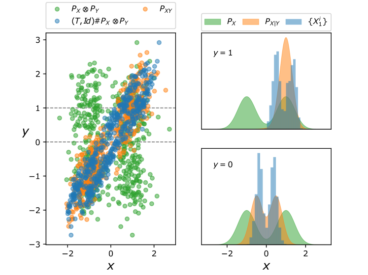
Figure 1: Numerical result for the bimodal example in Section V. Samples from the joint distribution $P_{XY}$, the independent coupling $P_{X}\otimes P_{Y}$, and the push-forward $(\nabla_{x}f,\text{Id})\#P_{X}\otimes P_{Y}$ are depicted in the left panel, where $f$ is an approximate solution to the variational problem. problem (4). The prior distribution $P_{X}$, along with the exact posterior distribution $P_{X|Y=y}$ and the approximated posterior distribution $\nabla_{x}f(\cdot,y)\#P_{X}$ for two values $y=0,1$ are depicted in the right panels.

VI Concluding remarks

The paper presents a variational characterization of the Bayes’s law using tools from optimal transportation theory. The variational formulation is used to derive the optimal transport EnKF algorithm, and propose novel generalizations of the EnKF algorithm to the non-Gaussian setting, utilizing ICNN and stochastic optimization algorithms. The paper presents preliminary numerical result that serve as proof of concept, while extensive numerical studies and comparison with other nonlinear filtering algorithms are subject of ongoing work.

-A Proof sketch of the proposition 1

The value of the objective function (III-A) is obtained using the quadratic form of the function $f(x,y;\theta)=\frac{1}{2}x^{T}Ax+x^{T}(Ky+b)$, and its convex conjugate

$$f^{*}(x,y;\theta)=\frac{1}{2}(x-Ky-b)^{T}A^{-1}(x-Ky-b)$$

The objective function is convex with respect to $\theta=\{A,K,b\}$ because, (i) the function $f(x,y;\theta)$ is linear in $\theta$, and (ii) $f^{*}(x,y;\theta)$ is a maximization over linear functions of $\theta$, hence convex. The solution to the optimization problem is obtained using the first-order optimality condition.

-B Proof sketch of the proposition 2

Express (18) as $f(x,y)=\frac{1}{2}\|x\|^{2}+\eta(x,y)$ where $\eta(x,y)=\phi(x)y+\psi(x)\Delta t$. Then, the convex conjugate of $f$ up to the fourth order in $\eta$ is

$$f^{*}(x,y) =\frac{1}{2}\|x\|^{2}-\eta(x,y)+\frac{1}{2}\|\nabla_{x}\eta(x,y)\|^{2}$$

$$-\frac{1}{2}\nabla_{x}\eta(x,y)^{T}\nabla_{x}^{2}\eta(x,y)\nabla_{x}\eta(x,y)$$

$$+\frac{1}{2}\|\nabla^{2}_{x}\eta(x,y)\nabla_{x}\eta(x,y)\|^{2}$$

The expression (20) is obtained using the form for $f$, the expansion of the convex conjugate $f^{*}$, and the observation model $Y=h(X)\Delta t+\sigma_{w}W_{\Delta t}$. The details are removed on the account of the space.

References

- [1] Brandon Amos, Lei Xu, and J Zico Kolter. Input convex neural networks. In Proceedings of the 34th International Conference on Machine Learning-Volume 70, pages 146–155. JMLR. org, 2017.
- [2] T. Bengtsson, P. Bickel, and B. Li. Curse of dimensionality revisited: Collapse of the particle filter in very large scale systems. In IMS Lecture Notes - Monograph Series in Probability and Statistics: Essays in Honor of David F. Freedman, volume 2, pages 316–334. Institute of Mathematical Sciences, 2008.
- [3] Kay Bergemann and Sebastian Reich. An ensemble kalman-bucy filter for continuous data assimilation. Meteorologische Zeitschrift, 21(3):213, 2012.
- [4] A. Beskos, D. Crisan, A. Jasra, and N. Whiteley. Error bounds and normalising constants for sequential Monte Carlo samplers in high dimensions. Advances in Applied Probability, 46(1):279–306, 2014.
- [5] Yann Brenier. Décomposition polaire et réarrangement monotone des champs de vecteurs. CR Acad. Sci. Paris Sér. I Math., 305:805–808, 1987.
- [6] Guillaume Carlier, Victor Chernozhukov, and Alfred Galichon. Vector quantile regression: an optimal transport approach. The Annals of Statistics, 44(3):1165–1192, 2016.
- [7] Yize Chen, Yuanyuan Shi, and Baosen Zhang. Optimal control via neural networks: A convex approach. arXiv preprint arXiv:1805.11835, 2018.
- [8] Y. Cheng and S. Reich. A McKean optimal transportation perspective on Feynman-Kac formulae with application to data assimilation. arXiv preprint arXiv:1311.6300, 2013.
- [9] D. Crisan and J. Xiong. Approximate McKean-Vlasov representations for a class of SPDEs. Stochastics, 82(1):53–68, 2010.
- [10] F. Daum, J. Huang, and A. Noushin. Exact particle flow for nonlinear filters. In SPIE Defense, Security, and Sensing, pages 769704–769704, 2010.
- [11] F. Daum, J. Huang, and A. Noushin. Generalized Gromov method for stochastic particle flow filters. In SPIE Defense+ Security, pages 102000I–102000I. International Society for Optics and Photonics, 2017.
- [12] A. M. Doucet, A.and Johansen. A tutorial on particle filtering and smoothing: Fifteen years later. Handbook of Nonlinear Filtering, 12:656–704, 2009.
- [13] Tarek A El Moselhy and Youssef M Marzouk. Bayesian inference with optimal maps. Journal of Computational Physics, 231(23):7815–7850, 2012.
- [14] G. Evensen. Data Assimilation. The Ensemble Kalman Filter. Springer-Verlag, New York, 2006.
- [15] Abhishek Halder and Tryphon T Georgiou. Gradient flows in uncertainty propagation and filtering of linear Gaussian systems. In 2017 IEEE 56th Annual Conference on Decision and Control (CDC), pages 3081–3088. IEEE, 2017.
- [16] Abhishek Halder and Tryphon T Georgiou. Gradient flows in filtering and Fisher-Rao geometry. In 2018 Annual American Control Conference (ACC), pages 4281–4286. IEEE, 2018.
- [17] Abhishek Halder and Tryphon T Georgiou. Proximal recursion for the wonham filter. In 2019 IEEE 58th Conference on Decision and Control (CDC), pages 660–665. IEEE, 2019.
- [18] Jeremy Heng, Arnaud Doucet, and Yvo Pokern. Gibbs flow for approximate transport with applications to bayesian computation. arXiv preprint arXiv:1509.08787, 2015.
- [19] Richard Jordan, David Kinderlehrer, and Felix Otto. The variational formulation of the Fokker–Planck equation. SIAM journal on mathematical analysis, 29(1):1–17, 1998.
- [20] Nikola Kovachki, Ricardo Baptista, Bamdad Hosseini, and Youssef Marzouk. Conditional sampling with monotone gans. arXiv preprint arXiv:2006.06755, 2020.
- [21] R. S. Laugesen, P. G. Mehta, S. P. Meyn, and M. Raginsky. Poisson’s equation in nonlinear filtering. SIAM Journal on Control and Optimization, 53(1):501–525, 2015.
- [22] Ashok Makkuva, Amirhossein Taghvaei, Sewoong Oh, and Jason Lee. Optimal transport mapping via input convex neural networks. In International Conference on Machine Learning, pages 6672–6681. PMLR, 2020.
- [23] Youssef Marzouk, Tarek Moselhy, Matthew Parno, and Alessio Spantini. An introduction to sampling via measure transport. arXiv preprint arXiv:1602.05023, 2016.
- [24] Diego A Mesa, Justin Tantiongloc, Marcela Mendoza, Sanggyun Kim, and Todd P. Coleman. A distributed framework for the construction of transport maps. Neural computation, 31(4):613–652, 2019.
- [25] Gabriel Peyré, Marco Cuturi, et al. Computational optimal transport: With applications to data science. Foundations and Trends® in Machine Learning, 11(5-6):355–607, 2019.
- [26] Deep Ray, Harisankar Ramaswamy, Dhruv V Patel, and Assad A Oberai. The efficacy and generalizability of conditional GANs for posterior inference in physics-based inverse problems. arXiv preprint arXiv:2202.07773, 2022.
- [27] Patrick Rebeschini, Ramon Van Handel, et al. Can local particle filters beat the curse of dimensionality? The Annals of Applied Probability, 25(5):2809–2866, 2015.
- [28] S. Reich. A dynamical systems framework for intermittent data assimilation. BIT Numerical Analysis, 51:235–249, 2011.
- [29] Sebastian Reich. A nonparametric ensemble transform method for Bayesian inference. SIAM Journal on Scientific Computing, 35(4):A2013–A2024, 2013.
- [30] Sebastian Reich. Data assimilation: The Schrödinger perspective. Acta Numerica, 28:635–711, 2019.
- [31] Sebastian Reich and Colin Cotter. Probabilistic forecasting and Bayesian data assimilation. Cambridge University Press, 2015.
- [32] Yuyang Shi, Valentin De Bortoli, George Deligiannidis, and Arnaud Doucet. Conditional simulation using diffusion schr” odinger bridges. arXiv preprint arXiv:2202.13460, 2022.
- [33] Ali Siahkoohi, Gabrio Rizzuti, Mathias Louboutin, Philipp A Witte, and Felix J Herrmann. Preconditioned training of normalizing flows for variational inference in inverse problems. arXiv preprint arXiv:2101.03709, 2021.
- [34] Alessio Spantini, Ricardo Baptista, and Youssef Marzouk. Coupling techniques for nonlinear ensemble filtering. arXiv preprint arXiv:1907.00389, 2019.
- [35] A. Taghvaei and P. G. Mehta. An optimal transport formulation of the linear feedback particle filter. In American Control Conference (ACC), 2016, pages 3614–3619. IEEE, 2016.
- [36] Amirhossein Taghvaei and Prashant G Mehta. An optimal transport formulation of the ensemble kalman filter. IEEE Transactions on Automatic Control, 66(7):3052–3067, 2020.
- [37] Amirhossein Taghvaei and Prashant G Mehta. Optimal transportation methods in nonlinear filtering: The feedback particle filter. arXiv preprint arXiv:2102.10712, 2021.
- [38] C. Villani. Topics in Optimal Transportation, volume 58. American Mathematical Soc., 2003.
- [39] T. Yang, R. S. Laugesen, P. G. Mehta, and S. P. Meyn. Multivariable feedback particle filter. Automatica, 71:10–23, 2016.
- [40] T. Yang, P. G. Mehta, and S. P. Meyn. Feedback particle filter. IEEE Transactions on Automatic Control, 58(10):2465–2480, October 2013.