Detailed Chemical Abundances of Star Clusters in the Large Magellanic Cloud

Abstract

We derive the first detailed chemical abundances of three star clusters in the Large Magellanic Cloud (LMC), NGC1831 (436$\pm$22 Myr), NGC1856 (350$\pm$18 Myr) and [SL63]268 (1230$\pm$62 Myr) using integrated-light spectroscopic observations obtained with the Magellan Echelle spectrograph on Magellan Baade telescope. We derive [Fe/H], [Mg/Fe], [Ti/Fe], [Ca/Fe], [Ni/Fe], [Mn/Fe], [Cr/Fe] and [Na/Fe] for the three clusters. Overall, our results match the LMC abundances obtained in the literature as well as those predicted by detailed chemical evolution models. For clusters NGC1831 and NGC1856, the [Mg/Fe] ratios appear to be slightly depleted compared to [Ca/Fe] and [Ti/Fe]. This could be hinting at the well-known Mg-Al abundance anti-correlation observed in several Milky Way globular clusters. We note, however, that higher signal-to-noise observations are needed to confirm such a scenario, particularly for NGC 1831. We also find a slightly enhanced integrated-light [Na/Fe] ratio for cluster [SL63]268 compared to those from the LMC field stars, possibly supporting a scenario of intracluster abundance variations. We stress that detailed abundance analysis of individual stars in these LMC clusters is required to confirm the presence or absence of MSPs.

1 Introduction and Motivation

Star clusters are key observational tools for understanding stellar astrophysics and evolution. Determining the abundances of elements resulting from different nucleosynthetic processes such as Type I supernovae (producing Fe-peak elements, for instance Sc, V, Cr, Mn , Fe, Co and Ni), winds from evolved stars, core collapse supernovae (producing $\alpha$-elements: O, Ne, Mg, Si S, Ar, Ca and Ti), can provide us with information about these complex mechanisms. Detailed chemical abundances of stellar populations are also used to uncover information about the chemical enrichment history of the host galaxy (McWilliam, 1997; Worthey, 1998; Matteucci, 2003).
In order to reveal the chemical enrichment history of a galaxy, we need accurate ages and abundances of star clusters. Several studies (e.g. Asa’d et al., 2016; Asa’d & Goudfrooij, 2020; Goudfrooij & Asa’d, 2021; Asa’d et al., 2021, 2022, and references therein) discussed the precision of age estimates of star clusters based on integrated spectra.
Knowing the abundances of star clusters is also crucial in understanding their own formation and evolution, especially with the discovery of the Multiple Stellar Populations (MSP) phenomenon defined as star-to-star variations in the inferred abundances of light elements (He, C, N, O, Na, Al; e.g. Carretta et al., 2009). The discovery of MSPs in stellar clusters continues to challenge our view of star clusters as being simple stellar populations. This phenomenon is one of the most puzzling ones in the field of star clusters and it is still not well understood.

The Large Magellanic Cloud (LMC) is a nearby (51 kpc; Wagner-Kaiser & Sarajedini, 2017) irregular galaxy. Due to its proximity, the LMC is an ideal laboratory for studying star clusters in great detail. Although the stellar clusters in the LMC resemble the Galactic globular clusters (GCs) in both shape and population, these extragalactic clusters have ages similar to the open clusters of our galaxy (van den Bergh, 1991). Old globular clusters have proven to be useful tools for tracing both the early formation and the star formation history of the LMC (Olszewski et al., 1991; Geisler et al., 1997; Hill et al., 2000). These studies and others show that metallicity and age distributions of the cluster population in the LMC are indeed bimodal, with a well-defined gap between 3-4 Gyr and 10-12 Gyr ago. This bimodality has been interpreted as the signature of two main bursts of star formation, an early one producing the 12-15 Gyr old clusters and a more recent one taking place 3 Gyr ago. The most recent burst of star formation was possibly triggered by tidal interaction of the LMC with the Milky Way (See discussion in Matteucci, 2012). However, we note that recently Gatto et al. (2020) identified 16 candidate clusters with estimated ages falling in the so-called age gap, located in the outskirts of the LMC.

Additionally, the confirmation of the presence of MSPs in the GCs in this extragalactic environment through both photometric and spectroscopic studies, make the LMC even more intriguing (see e.g. Milone et al., 2009; Piatti, 2020, and references within). The LMC is unique compared to the MW because it allows for the exploration of the presence of MSPs not only in ancient GC but also in intermediate-age clusters. A detailed review of these relatively new results is provided in Bastian & Lardo (2018).

In order to get the full picture of the star formation history and chemical evolution of galaxies, we need to combine existing studies of chemical abundances of old stellar population with those of younger populations. At present there are several different tools available to study the present-day chemical state of galaxies, such as measurements of H II regions (Searle, 1971; Rubin et al., 1994; Stasińska, 2005), analysis of the integrated light of star clusters (Larsen et al., 2012; Hernandez et al., 2017, 2018a, 2019; Bastian et al., 2019, 2020) and analysis of evolved massive stars (See for example Davies et al., 2015; Origlia et al., 2019; Asa’d et al., 2020). In an effort to further investigate the chemical evolution of the LMC and its stellar clusters, we performed a detailed chemical study of three young massive clusters (YMCs) in this nearby irregular galaxy.

In this paper we present the analysis of the integrated light of the YMCs NGC1831, NGC1856 and [SL63]268. We measure for the first time detailed abundances of $\alpha$ (Ti, Mg, and Ca), light (Na), and Fe-peak elements (Ni, Mn and Cr) in these three extragalactic clusters. The paper is organized as follows: in Section 2 we describe the spectroscopic observations and data reduction; in Sections 3 and 4 we detail the integrated-light analysis technique used to infer the chemical abundances, and the stellar atmospheric models used in generating the synthetic integrated-light spectra, respectively; in Sections 5 and 6 we present our results and discuss our findings in the context of chemical evolution and MSPs; and lastly in Section 7 we summarize our conclusions.

2 Observations and Data Reduction

The observations analyzed as part of this work include three LMC clusters in the age range from 300 Myr to 1.5 Gyr, observed with the 6.5 m Magellan Baade telescope in 2016 November, using the intermediate resolution Magellan Echelle (MagE, Marshall et al. 2008) spectrograph. We used for our observation the 0.5 arcsec wide slit; with resolution (R) =7000; and wavelength range: 3300 $<\lambda$(Å) $<$ 9500. We used the scan mode with 2$\times$900sec exposures for NGC1831, 2$\times$900sec exposures for NGC1856 and 2$\times$1800sec exposures for [SL63]268. The signal-to-noise S/N ratio for the redder side of [SL63]268 monotonically increases from about 40 Å^-1 to 80 Å^-1 at wavelength between 4000 Å and 6700 Å, while for the other two clusters it stays nearly constant over wavelength at 60 Å^-1 for NGC 1831 and 160 Å^-1 for NGC 1856.

We refer the interested reader to Chilingarian & Asa’d (2018) for more details about the observations. In order to collect an integrated spectrum, we scanned a cluster across the slit using the nonsideral tracking. The data reduction was done by developing a dedicated data reduction pipeline that merges Echelle orders and produces a sky-subtracted flux-calibrated two-dimensional spectrum corrected for telluric absorption and its corresponding flux uncertainty frame. The spectrum is then collapsed along the slit to obtain a one-dimensional flux-calibrated data product in the wavelength range 3700$<\lambda\>$ (Å) $<6800$.

3 Method

We use the software developed for GCs by Larsen et al. (2012), and later applied to YMCs by Hernandez et al. (2017), to obtain detailed abundances for our LMC sample. This technique relies on existing age estimates for the stellar populations under study, to select the best initial isochrone.

We generate theoretical PARSEC isochrones (Bressan et al., 2012) adopting the ages estimated for our sample by Chilingarian & Asa’d (2018), and an initial metallicity of [m$/$H] = -0.4. We adopt a Salpeter (1955) initial mass function (IMF) and a lower mass limit of 0.4 M_⊙ when extracting the stellar atmospheric parameters (e.g., effective temperature, surface gravity, mass) from the isochrones. Lastly, we account for the microturbulent velocity component, $v_{t}$, assigning different values depending on the effective temperature ($T_{\rm eff}$) of the individual stars: $v_{t}$ = 2 km s^-1 for stars with $T_{\rm eff}<$ 6000 K, $v_{t}$ = 4 km s^-1 for stars with 6000 $<T_{\rm eff}<$ 22 000 K, and $v_{t}$ = 8 km s^-1 for stars with $T_{\rm eff}>$ 22 000 K (Hernandez et al., 2017, 2018a).

We note that the analysis of integrated-light observations of stellar clusters is subject to stochastic fluctuations in the number of stars of a given stellar type falling in the scanned area. The effects of random IMF sampling in the type of analysis described here have been assessed in previous studies (e.g., Larsen et al., 2012, 2017). Larsen et al. (2017) has tested the uncertainties introduced by the stochastic sampling of the HRD. They produced Monte-Carlo simulations where the same number of stars as those present within the scanned areas were sampled at random from the full CMDs, and performed a similar abundance analysis on these randomly sampled CMDs. Overall, the stochastic sampling experiment in Larsen et al. (2017) indicated that the stochastically induced (1-$sigma$) uncertainty on overall metallicities is $<$ 0.1 dex.

Using the software by Larsen et al. (2012) we first obtain an estimate of the radial velocity of the individual star cluster, by fitting small wavelength windows of 200Å from 4000Å to 6200Å. This wavelength range was selected as it provided a reasonable number of bins and excluded the lowest S/N regions at wavelengths $\lesssim$4000 Å. We estimate the mean radial velocities and adopt these values for the rest of our abundance analysis (see the first row in Table 1). Our estimated values are comparable to those of Chilingarian & Asa’d (2018), who obtained radial velocities of 278.8$\pm$0.6 km/s, 268.6$\pm$0.2 km/s and 266.0$\pm$0.5 km/s for NGC1831, NGC1856 and [SL63]268, respectively.

To match the resolution between the synthetic integrated-light models and that of the spectroscopic observations, we fit for the best Gaussian dispersion, $\sigma_{\rm sm}$. The scaling of the synthetic spectrum is determined by fitting the ratio of the synthetic and observed spectra with a spline or polynomial functions, depending on the size of the wavelength bin. In Section 3.1, we present a brief discussion on the sensitivity of our analysis to the scaling procedure.

In this work, [Z] is defined as a scaling parameter relative to solar composition and applied to all of the specified abundances. This means that [Z] is a measure of the integrated abundances of the different chemical elements. In the current work we have adopted the solar composition from Grevesse & Sauval (1998).

We begin the abundance analysis by simultaneously fitting for the best $\sigma_{\rm sm}$ and [Z]. We fit each spectrum using 200-Å  bins scanning the wavelength range between 4000 Å  and 5800 Å . This wavelength region provided sufficient information for deriving the initial scaling parameter, [Z], and at the same time allowed us to exclude the lower S/N regions at $\lesssim$4000 Å. A direct comparison is made between the model spectrum and the science observations by performing a $\chi^{2}$ minimization. The continua of the model and observed spectra are matched using a cubic spline with three knots. The process is repeated modifying the variables accordingly until the best match is determined.

We then proceed to measuring the abundance of a number of individual elements starting with those having the highest number of lines, while keeping the overall metallicity and the smoothing parameters fixed.

We first measure Fe then Ti and Ca, followed by the rest of the elements. We masked the bad pixels around 6300 Å  for NGC1831, NGC1856 and [SL63]268. We used the optimised wavelength windows tailored for each element introduced by Hernandez et al. (2017) in order to ameliorate the effects of strong blending.
Similar to the procedure followed for the overall metallicity estimation, we use a cubic spline with three knots to match the continua of the model and observed spectra for windows $\geq$ 100 Å . For bins narrower than 100 Å  we use a first-order polynomial instead.

3.1 Scaling of the continuum level

Larsen et al. (2012, 2014) discuss extensively the proper scaling of the continuum level. To avoid problematic continuum placements due to weak features present in the data, they have identified continuum regions in the observed spectrum of Arcturus, and use only these regions free of absorption features when scaling the model and science observations. Similar to the analysis of intermediate-resolution observations of YMCs in Hernandez et al. (2017) we made use of these pre-defined continuum regions when scaling the model and observations.

To get a better sense of the sensitivity of our analysis to the continuum scaling procedure, we estimated the overall metallicities for NGC 1831, the cluster with the lowest S/N values in our sample, applying three different methods: (1) our standard method of using the predefined continuum regions from Larsen et al. (2012, 2014) and Hernandez et al. (2017), and applying a spline function with three knots to determine the scaling of the model spectrum, (2) using the predefined continuum regions, along with a first order polynomial to determine the scaling of the model spectrum, (3) applying no restrictions on the continuum pixels and using a spline function with three knots to determine the scaling of the model spectrum. We found differences of 0.05 dex in the overall metallicities inferred using method (2), compared to the value obtained with our standard approach (method 1). Similarly, we found differences of 0.06 dex when applying method (3), in comparison to our adopted approach. Given that the overall S/N values for the other two clusters are higher, these differences provide an upper limit to the uncertainties introduced by the continuum scaling procedure.

4 Models

The Larsen et al. (2011) technique produces synthetic integrated-light spectra by co-adding individual spectra generated for each of the stars in the cluster. The synthetic spectra are generated by creating a series of high spectral resolution models that include all evolutionary stages present in the star cluster. The software first computes atmospheric models using ATLAS9 (Kurucz, 1970) for stars with T${}_{\rm eff}>$ 3500 K and using MARCS (Gustafsson et al., 2008) for stars with T${}_{\rm eff}<$ 3500 K.
The atmospheric models are then used to create synthetic spectra with SYNTHE (Kurucz & Furenlid, 1979; Kurucz & Avrett, 1981) for the ATLAS9 models and TURBOSPECTRUM (Plez, 2012) for MARCS models. The model spectra are created at high resolution of R = 500,000 and then degraded to match the observations. For the synthetic spectral computations, we use the line lists by Castelli & Hubrig (2004) which include hyperfine splitting for a few Mn I lines.

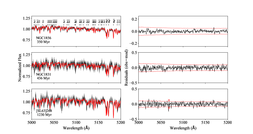
Figure 1: Left: Synthesis fits for our sample of YMCs in the LMC. In black we show the MagE spectroscopic observations, along with their uncertainties in grey. In red we show the model fit. We indicate the cluster name and the assumed age below the corresponding spectra. Right: We display the residuals in black. The red dashed lines indicate the 3$\sigma$ error spectrum.

5 Results

In Figure 1 we show our synthesis fits for all three clusters, along with their residuals. The chemical abundances obtained are included in Tables 3, 4 and 5 where we list the wavelength bins used in the abundance measurement of each element, the best fit abundance and their corresponding uncertainties calculated from the $\chi^{2}$ fit. We used five bins for Fe, four bins for Ca, three bins for Ti, four bins for Cr, five bins for Ni, two bins for Na and one bin for each of Mg and Mn. The tables show that for several bins the software was unable to converge to a final abundance. Table 1 presents the weighted average abundances of our clusters and their uncertainties obtained by dividing the standard deviation by $\sqrt{N-1}$, where N is the the number of wavelength bins used for obtaining each abundance. Here $[$Fe/H$]=$ Fe + [Z], where Fe is the mean iron abundance estimated for each wavelength bin listed in Tables 3, 4 and 5. The other listed elements [X/Fe] were calculated using the equation [X/Fe] = [X/H] - [Fe/H], where [X/H] = X + [Z], and X is the weighted average abundance of element X estimated for each wavelength bin listen in Tables 3, 4 and 5.

Table 1: Our Results

	NGC1831	NGC1856	[SL63]268
RV (km s-1)	290$\pm$7	279$\pm$4	278$\pm$4
$\sigma_{\rm sm}$ (km s-1)	23.9	26.9	24.6
$[$Z$]$	-0.418$\pm$0.07	-0.574$\pm$0.06	-0.51$\pm$0.04
$[$Fe/H$]$	-0.375$\pm$0.12	-0.455$\pm$0.11	-0.506$\pm$0.1
$[$Ca/Fe$]$	0.814$\pm$0.41	0.375$\pm$0.2	-0.277$\pm$0.39
$[$Na/Fe$]$	0.023$\pm$0.77	0.093$\pm$0.38	0.357$\pm$0.08
$[$Mg/Fe$]$	0.082$\pm$0.16	-0.074$\pm$0.13	0.07$\pm$0.11
$[$Ti/Fe$]$	0.547$\pm$0.42	0.262$\pm$0.2	0.233$\pm$0.19
$[$Cr/Fe$]$	0.002$\pm$0.5	0.132$\pm$0.16	0.111$\pm$0.0
$[$Mn/Fe$]$	0.323$\pm$0.38	-0.263$\pm$0.32	-0.199$\pm$0.21
$[$Ni/Fe$]$	0.318$\pm$0.5	-0.194$\pm$0.08	-0.224$\pm$0.41

6 Discussion

6.1 Comparing our Results

In this section, we compare our results with those obtained from previous studies. In Table 2 we list our results for [Fe/H] and [Mg/Fe], as well as those obtained by Chilingarian & Asa’d (2018).
Chilingarian & Asa’d (2018) used nbursts (Chilingarian et al., 2007), a full spectrum fitting tool, to obtain the age, Z and [Mg/Fe]. [Fe/H] is calculated using the equation given in Chilingarian & Asa’d (2018):

$$[\mathrm{Fe/H}]=[\mathrm{Z/H}]-0.75[\mathrm{\alpha/Fe}]$$ (1)

where [$\alpha$/Fe] is the obtained [Mg/Fe] from nbursts. Overall, the results match reasonably well, with the exception of [Mg/Fe] for NGC1856, where we measure a slightly more depleted ratio than Chilingarian & Asa’d (2018).

Table 2: Ages, metallicities and abundances of our sample

Object	Age${}_{\rm Lit}^{1}$	[Fe/H]${}_{\rm Lit}^{2}$	[Fe/H]	[Mg/Fe]${}_{\rm Lit}^{3}$	[Mg/Fe]
NGC1831 (catalog )	436$\pm$22	-0.39$\pm$0.05	-0.38$\pm$0.12	0.09$\pm$0.06	0.08$\pm$0.16
NGC1856 (catalog )	350$\pm$18	-0.47$\pm$0.02	-0.46$\pm$0.11	0.18$\pm$0.03	-0.07$\pm$0.13
[SL63]268 (catalog )	1230$\pm$62	-0.58$\pm$0.03	-0.51$\pm$0.1	0.09$\pm$0.02	0.07$\pm$0.11

1. The ages in Myr from Chilingarian & Asa’d (2018) are the ones obtained when counting for alpha elements. 2. [Fe/H] were calculated using Z and [alpha/Fe] from table 2 in Chilingarian & Asa’d (2018) and corrected equation 1. 3. [Mg/Fe] are the values of [alpha/Fe] listed in table 2 in Chilingarian & Asa’d (2018) as these values were calculated based on Mg only. [Fe/H] and [Mg/Fe] are measured in dex.

In Figure 2, we show our inferred YMC abundances along with those from field stars in the LMC and theoretical models. The abundance ratios inferred as part of this work are shown as different symbols (navy for NGC1831, red for NGC1856 and green for [SL63]268). The orange and light blue dots are the literature data from field stars in the LMC bar and inner disc abundances, respectively, presented by Van der Swaelmen et al. (2013) and the black line is the theoretical LMC model. We note that the model was originally scaled to the solar abundances of Asplund et al. (2009), however, we homogenize the model and measured abundances to the single abundance scale of Grevesse & Sauval (1998). The chemical evolution model adopted for the LMC is similar to that of Calura et al. (2003). The evolution of the gas abundances of several chemical species is computed in detail. The chemical enrichment from supernovae of all types (II, Ia, Ib, Ic) as well as from AGB stars is considered together with stellar lifetimes.

For the history of star formation (SF) of the LMC we assume two main bursts, the first between 0 and 5 Gyr and the second at 12 Gyr. The efficiency of SF is 0.1 Gyr^-1 during the bursts and 0.001 Gyr^-1 in between. We adopt the duration and number of bursts as suggested by Harris & Zaritsky (2009) and fix the star formation efficiency to reproduce the abundance pattern, the present time mass of gas and stars as well as supernovae rates.

The star formation rate is defined as :

$$\psi(t)=\nu M_{gas}$$ (2)

where $\nu$ is the efficiency of star formation. We assume that the LMC assembled by infall of primordial gas with the following law:

$$\dot{M}_{gas,infall}=aX_{i}e^{-t/\tau}$$ (3)

where $a$ is a parameter tuned to reproduce the total present time mass of LMC ($M_{LMC}=6$x$10^{6}$), $X_{i}$ is the abundance of the element $i$ in the infalling gas and $\tau=0.5$ Gyr is the infall timescale.

The model considers also gas outflow from the galaxy when the thermal energy produced by SNe and stellar winds equates the binding energy of gas (see Bradamante et al. 1998 for a detailed discussion).

The wind rate is expressed as being proportional to the star formation rate:

$$\dot{M}_{outflow}=-\omega\psi(t)$$ (4)

where $\omega=0.25$ is the mass loading factor and is adimensional.

For the stellar yields we adopt those from Karakas (2010) for the chemical enrichment from low and intermediate mass stars ($0.8\leq M/M_{\odot}\leq 8$) and from Kobayashi et al. (2006) for massive stars ($M>8M_{\odot}$). For Type Ia SNe, here assumed to originate from white dwarfs in binary systems, we adopt the yields from Iwamoto et al. (1999).

The elements considered in this paper are mainly formed in core-collapse SNe (II, Ib, Ic) and Type Ia SNe, so the contribution from AGBs is negligible. It is worth noting that the yields of some elements, such as Ti and Cr, are still very uncertain, as shown by previous works (e.g. Romano et al. 2010; Matteucci 2021) and to reproduce the data of the solar vicinity one needs to change them arbitrarily. The reason for such uncertainties can be found in uncertain nuclear reaction rates and treatment of convection in stellar models.

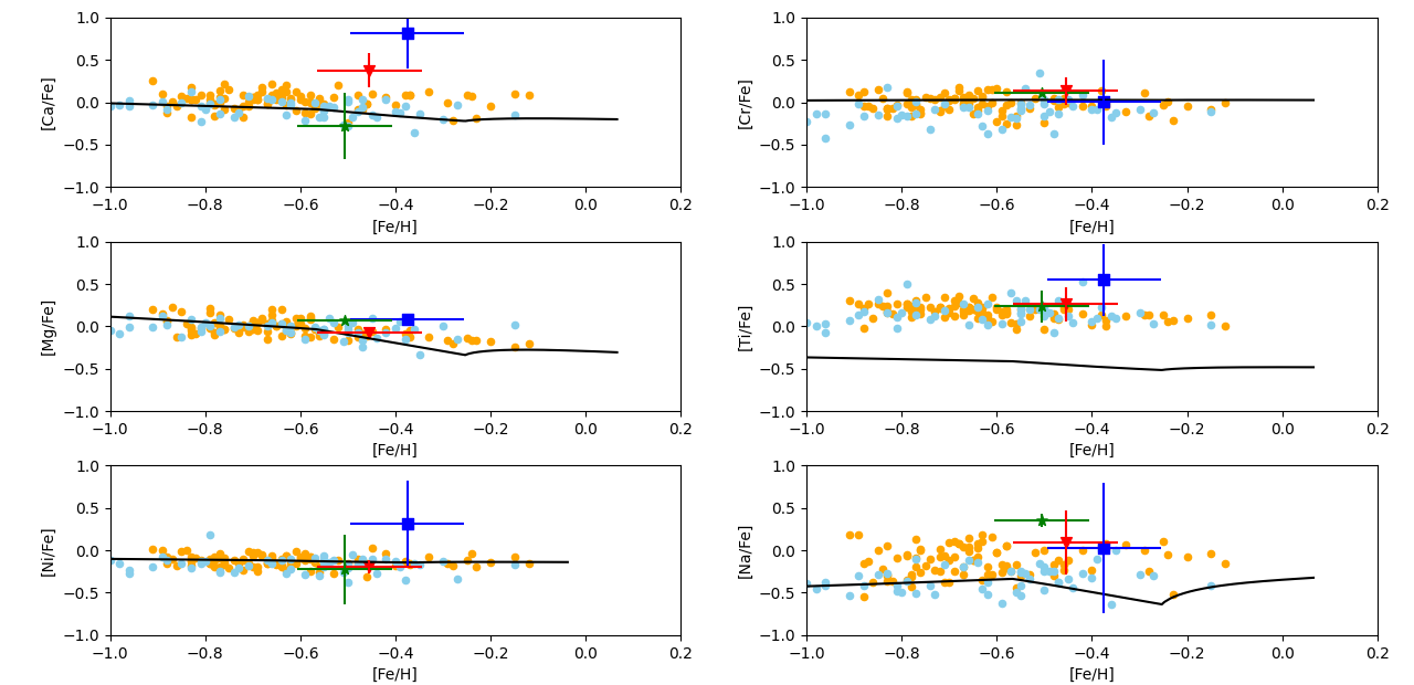
Figure 2: Abundance ratios as a function of [Fe/H]. The abundance ratios inferred as part of this work are shown as diamonds (navy square for NGC1831, red triangle for NGC1856 and green star for [SL63]268). The orange and light blue dots are the literature data from field stars in the LMC bar and inner disc abundances, respectively, presented by Van der Swaelmen et al. (2013). We show with a solid black line the chemical evolution models for the LMC.

Overall, our abundance ratios agree with those predicted by the theoretical model for the available elements. Currently, there are no theoretical models available for Mn, which prevents us from comparing our abundances against predicted values. The agreement between our inferred abundances and those predicted by the chemical evolution model supports a scenario where the star formation history of the LMC would involve two main bursts. Additionally, the work presented here shows that integrated spectra of star clusters are reliable tools for studying the chemical enrichment history for distant galaxies (where resolved data cannot be obtained).
A comparison between our inferred abundances and those measured by Van der Swaelmen et al. (2013) for the field stars in the LMC shows that the ratios for Ca, Ni and Ti for NGC1831 are on the high side of the envelope of observed abundances in field. For these three elements we have compared the adopted oscillator strength values (log gf) from the study by Van der Swaelmen et al. (2013) and those used in our analysis. We find no differences between the log gf values for the Ti and Ni lines. For Ca we identify differences of the order of <0.1 dex. Overall, these differences, or the absence of such, most likely indicate that the abundance differences between those from NGC1831 and the field stars are not due to the adopted log gf values.
We note that from our sample of YMCs, the observations of NGC1831 showed the lowest S/N. This is also reflected in the higher uncertainties for the abundances of this YMC (for example $\sim$0.4 dex for [Ca/Fe]), compared to those for NGC1856 and [SL63]268. To confirm if the enhancement in Ca is intrinsic to the YMC NGC1831 in Figure 3 we overplot the Ca lines for NGC1831 and compare them with those for NGC1856. We chose to compare the spectroscopic observations of these two clusters as they have similar ages and metallicities. Figure 3 not only shows that NGC1831 exhibits stronger Ca lines than NGC1856, but it also contrasts the differences in S/N values between the two different datasets.

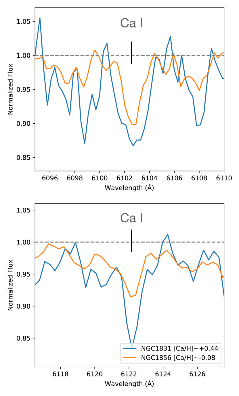
Figure 3: Ca spectral lines for NGC1831 (blue) and NGC1856 (orange).

6.2 Multiple Populations

It has been firmly established that Galactic GCs host MSPs inferred through star-to-star variations in the abundances of some light elements (e.g., He, C, N, O, Na, Al). However, in spite of many observational and theoretical studies, the physical origin of MSPs is still debated. Several scenarios have been proposed to explain this phenomenon, with most implying multiple epochs of star-formation within the cluster; however, none of these scenarios have fully succeeded to reproduce the increasing number of observations obtained in the past decade. Additionally, if YMCs are the young analogs of GCs, we expect to find MSPs in these young stellar populations. We note, however, that MSPs have not been detected in YMCs younger than 2 Gyr (Bastian & Lardo, 2018; Martocchia et al., 2021).

Studies have found intra-cluster Mg variations in several GCs in the MW (see review by Gratton et al., 2004; Bastian & Lardo, 2018). It is possible that these same intra-cluster variations in Mg might be detected in integrated-light studies of GC as (1) lower [Mg/Fe] ratios when compared to those from field stars (Larsen et al., 2014), or (2) lower [Mg/Fe] compared to other [$\alpha$/Fe] ratios for the same cluster (Colucci et al., 2009; Larsen et al., 2012). In the context of item (1), the middle left panel show that the distribution of [Mg/Fe] is compatible with the Mg abundances of field stars , however, in the context of item (2), our results in Table 1 show lower [Mg/Fe] ratios compared to those from [Ca/Fe] and [Ti/Fe] for YMCs NGC1831 and NGC1856 which might be an indication of the presence of MSPs. The upper limit of the [Mg/Fe] ratio for NGC1831 when errors are taken into account is 0.242 dex, which is still less than the lower limit of [Ca/Fe] ratio (0.404 dex), but more than the lower limit of [Ti/Fe] ratio (0.127 dex). For NGC1856 however, the upper limit of the [Mg/Fe] ratio within the error range (0.056 dex) is still significantly less than the lower limit of [Ca/Fe] and [Ti/Fe] ratios (0.175 dex and 0.462 dex, respectively).

In addition to Mg, Na has also exhibited star-to-star variations in Galactic GCs (Gratton et al., 2004). These variations in Na abundances are observed as significantly elevated [Na/Fe] ratios in integrated-light studies of GCs when compared to those of field stars (Colucci et al., 2009; Larsen et al., 2014; Hernandez et al., 2018b; Bastian et al., 2019, 2020). To further investigate the possibility of MSPs in our sample of YMCs, we estimate the Na abundances. For this we analyzed two wavelength bins covering several Na lines. The low S/N observations for NGC 1831 made it very challenging to accurately measure the Na abundances from these two wavelength bins. This is reflected in the large uncertainties of our inferred [Na/Fe] ratio for this particular cluster. In Figure 4 we display the best fit models and show with dashed vertical lines the location of the Na lines. We highlight that the Na doublet in the 6148-6168 Å  wavelength bin is rather weak (log gf $=$ $-$1.228, compared to log gf = $-$0.452 for Na I at 5688 Å), with one of the lines being blended with a much stronger Ca line.
In the lower right panel of Figure 2 we compare our inferred [Na/Fe] ratios for all three clusters, with those from field stars by Van der Swaelmen et al. (2013). Overall, this panel shows that the [Na/Fe] ratio is slightly more enhanced in cluster [SL63]268, compared to the abundances of the field stars. The inferred abundance of NGC 1856 appears to be on the upper envelope of observed abundances in the field. The mean value of the [Na/Fe] abundances of the field stars with -0.5 $<$[Fe/H] $<$-0.35 is -0.21, and the inferred values for NGC 1856 and [SL63]268 are 0.093$\pm$0.38 and 0.357$\pm$0.08, respectively. Based on the uncertainties of our measurement for cluster NGC 1856, we are unable to definitively confirm an enhancement in the [Na/Fe] ratio over the abundances of the field stars.

In the context of MSPs, the Na enhancement in [SL63]268 may be hinting at intracluster abundance variations in a cluster with an age slightly younger than 2 Gyr. [SL63]268 is younger than any LMC/SMC cluster in which evidence of MSPs (in the form of abundance variations, e.g. Martocchia et al. 2021) has been found so far. We note that in our sample we observe that [SL63]268 shows hints of Na variations but we find no evidence for Mg variations. On the other hand, NGC 1831 shows possible hints of variations in Mg, however, given the large uncertainties in our inferred [Na/Fe] ratio, we are unable to assert the presence or absence of an enhancement of Na over the abundances of the field stars. We highlight that depleted [Mg/Fe] ratios are not observed in all of the clusters in which Na variations are detected (Bastian & Lardo, 2018). Locally, only a few Galactic GCs have shown evidence of significantly depleted Mg (e.g., Mucciarelli et al., 2012; Carretta, 2014). More analysis is needed for this sample of LMC clusters to accurately investigate the MSP phenomenon.

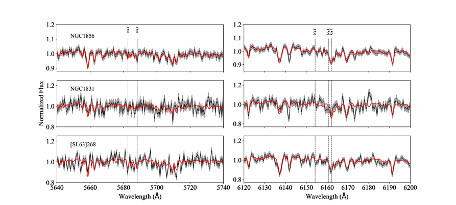
Figure 4: Best synthesis fits for our sample of YMCs. In black we show the MagE spectroscopic observations. In red we display the model fit. We show with dashed vertical lines the location of the Na lines.

7 Summary

In this work we perform the first detailed abundance analysis for three LMC YMCs observed with the Magellan Echelle spectrograph on Magellan Baade telescope. We follow the method described in Hernandez et al. (2017). We summarize below the results of our study:
(A) We derive [Fe/H], [Ti/Fe], [Ca/Fe], [Mg/Fe], [Ni/Fe], [Mn/Fe], [Cr/Fe] and [Na/Fe] abundances for NGC1831, NGC1856 and [SL63]268.
(B) Our results for [Fe/H] and [Mg/Fe] match reasonably with those derived by Chilingarian & Asa’d (2018).
(C) To the best knowledge, this study is the first to derive [Ti/Fe], [Ca/Fe], [Ni/Fe], [Mn/Fe], [Cr/Fe] and [Na/Fe] abundances for the three clusters of our sample.
(D) Overall our results match the LMC abundances obtained in the literature as well as the theoretical model.
(E) The nucleosynthesis of Ti element is very poorly known, further analysis is required to better constrain the theoretical models (See the model line in Figure 2).
(F) Our results from NGC1831 and NGC1856 show a possible depletion in the [Mg/Fe] abundance compared to [Ca/Fe] and [Ti/Fe].
(G) We also observe slightly enhanced [Na/Fe] ratios in cluster [SL63]268, when compared to the abundances of the field stars. This trend can be an indication of intracluster Na variations.
Based on observations, current models and theories suggest that the cutting limit between the occurrence and non-accordance of MSPs happens at ages of 2–3 Gyr, indicating that either the cluster age plays a dominant role in the establishment of MSPs or that the phenomenon is present only in low mass stars. The discovery of light element variations in clusters younger than 2 Gyr would provide new insights on the origin of this phenomenon and the parameters that play key roles in it. Although MSPs in stellar clusters younger than 2 Gyr is an intriguing possibility, we highlight that detailed abundance analysis of individual stars in these LMC clusters is required to confirm such a scenario.

Appendix A Inferred abundances

In Tables 3-5 we list the individual bin measurements for the YMCs studied here. To aid in the assessment of the degree of dispersion between the different bins for a given element, in Figures 5-8 we plot the inferred abundances as a function of wavelength.

Table 3: Chemical Abundances for NGC1831

Wavelength	Abundance	Error
[Z]
4000.00 - 4200.00	-0.173	0.102
4200.00 - 4400.00	-0.215	0.058
4400.00 - 4600.00	-0.447	0.070
4600.00 - 4800.00	-0.257	0.104
4800.00 - 5000.00	-0.680	0.085
5000.00 - 5200.00	-0.550	0.053
5200.00 - 5400.00	-0.605	0.085
5400.00 - 5550.00	-0.188	0.104
5600.00 - 5800.00	-0.646	0.084
Fe (dex)
4700.00 - 4800.00	+0.265	0.110
4900.00 - 5000.00	-0.146	0.142
5000.00 - 5100.00	+0.154	0.091
6100.00 - 6300.00	+0.217	0.086
6300.00 - 6340.00	-0.274	0.289
Ca (dex)
4445.00 - 4465.00	-0.633	0.559
6100.00 - 6128.00	+0.995	0.141
6430.00 - 6454.00	+0.676	0.354
6459.00 - 6478.00	+0.546	0.668
Cr (dex)
4580.00 - 4640.00	+0.026	0.239
4640.00 - 4675.00	+0.085	0.400
4915.00 - 4930.00	+0.084	0.651
6600.00 - 6660.00	-	-
Mg (dex)
5150.00 - 5200.00	+0.125	0.070
Mn (dex)
4750.00 - 4770.00	+0.366	0.350
Na (dex)
5670.00 - 5700.00	-0.531	0.536
6148.00 - 6168.00	+0.565	0.490
Ni (dex)
4700.00 - 4720.00	+1.215	0.191
4825.00 - 4840.00	-0.765	0.851
4910.00 - 4955.00	-	-
5075.00 - 5175.00	-0.422	0.218
6100.00 - 6200.00	+0.074	0.231
Ti (dex)
4650.0 - 4718.00	-0.265	0.421
4980.0 - 5045.00	+0.635	0.216
6584.0 - 6780.00	+0.865	0.267

Table 4: Chemical Abundances for NGC1856

Wavelength	Abundance	Error
[Z]
4000.00 - 4200.00	-0.381	0.062
4200.00 - 4400.00	-0.732	0.058
4400.00 - 4600.00	-0.792	0.066
4600.00 - 4800.00	-0.388	0.061
4800.00 - 5000.00	-0.543	0.048
5000.00 - 5200.00	-0.723	0.042
5200.00 - 5400.00	-0.700	0.050
5400.00 - 5550.00	-0.487	0.062
5600.00 - 5800.00	-0.421	0.051
Fe (dex)
4700.00 - 4800.00	+0.356	0.071
4900.00 - 5000.00	-0.115	0.070
5000.00 - 5100.00	+0.012	0.063
6100.00 - 6300.00	-0.024	0.060
6300.00 - 6340.00	+0.365	0.141
Ca (dex)
4445.00 - 4465.00	-	-
6100.00 - 6128.00	+0.307	0.168
6430.00 - 6454.00	+0.835	0.221
6459.00 - 6478.00	+0.385	0.533
Cr (dex)
4580.00 - 4640.00	+0.275	0.110
4640.00 - 4675.00	-0.086	0.291
4915.00 - 4930.00	+0.615	0.371
6600.00 - 6660.00	-0.388	1.017
Mg (dex)
5150.00 - 5200.00	+0.045	0.031
Mn (dex)
4750.00 - 4770.00	-0.144	0.294
Na (dex)
5670.00 - 5700.00	-0.072	0.287
6148.00 - 6168.00	+0.465	0.271
Ni (dex)
4700.00 - 4720.00	+0.105	0.230
4825.00 - 4840.00	-0.111	0.392
4910.00 - 4955.00	-	-
5075.00 - 5175.00	-0.055	0.101
6100.00 - 6200.00	-0.221	0.167
Ti (dex)
4650.00 - 4718.00	-0.004	0.209
4980.00 - 5045.00	+0.515	0.136
6584.00 - 6780.00	+0.428	0.177

Table 5: Chemical Abundances for [SL63]268

Wavelength	Abundance	Error
[Z]
4000.00 - 4200.00	-0.326	0.025
4200.00 - 4400.00	-0.453	0.032
4400.00 - 4600.00	-0.712	0.041
4600.00 - 4800.00	-0.534	0.047
4800.00 - 5000.00	-0.459	0.039
5000.00 - 5200.00	-0.512	0.027
5200.00 - 5400.00	-0.570	0.038
5400.00 - 5550.00	-0.561	0.054
5600.00 - 5800.00	-0.464	0.043
Fe (dex)
4700.00 - 4800.00	+0.191	0.055
4900.00 - 5000.00	-0.316	0.062
5000.00 - 5100.00	+0.046	0.050
6100.00 - 6300.00	+0.105	0.030
6300.00 - 6340.00	-0.005	0.131
Ca (dex)
4445.00 - 4465.00	-1.346	0.291
6100.00 - 6128.00	-0.144	0.125
6430.00 - 6454.00	+0.126	0.235
6459.00 - 6478.00	-0.846	0.451
Cr (dex)
4580.00 - 4640.00	+0.115	0.120
4640.00 - 4675.00	-	-
4915.00 - 4930.00	-	-
6600.00 - 6660.00	-	-
Mg (dex)
5150.00 - 5200.00	+0.074	0.031
Mn (dex)
4750.00 - 4770.00	-0.195	0.181
Na (dex)
5670.00 - 5700.00	+0.316	0.159
6148.00 - 6168.00	+0.433	0.202
Ni (dex)
4700.00 - 4720.00	-0.669	0.244
4825.00 - 4840.00	-1.126	0.731
4910.00 - 4955.00	-1.997	1.057
5075.00 - 5175.00	-0.356	0.092
6100.00 - 6200.00	+0.174	0.121
Ti (dex)
4650.00 - 4718.00	+0.081	0.185
4980.00 - 5045.00	+0.354	0.091
6584.00 - 6780.00	-0.188	0.211

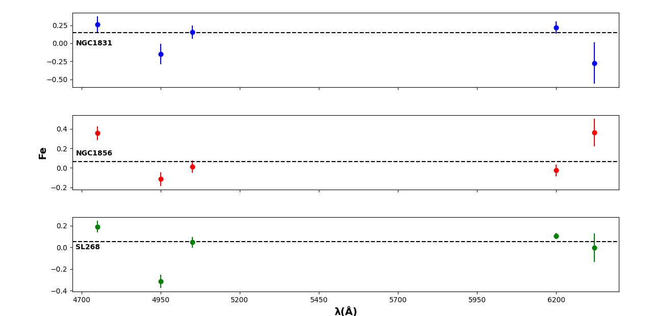
Figure 5: Fe abundances listed in Tables 3, 4 and 5 as a function of wavelength.The dotted line is the weighted average.

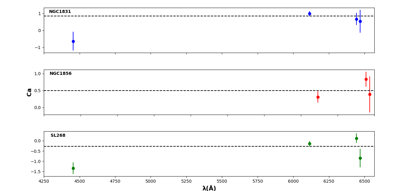
Figure 6: Ca abundances listed in Tables 3, 4 and 5 as a function of wavelength.The dotted line is the weighted average.

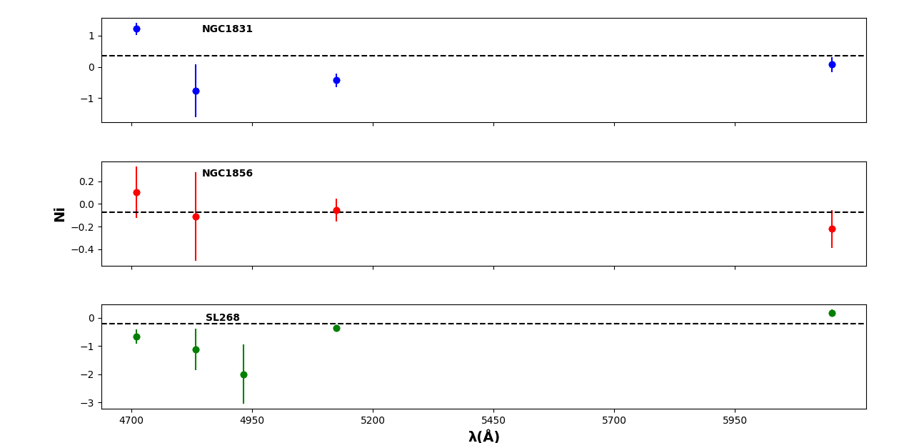
Figure 7: Ni abundances listed in Tables 3, 4 and 5 as a function of wavelength. The dotted line is the weighted average.

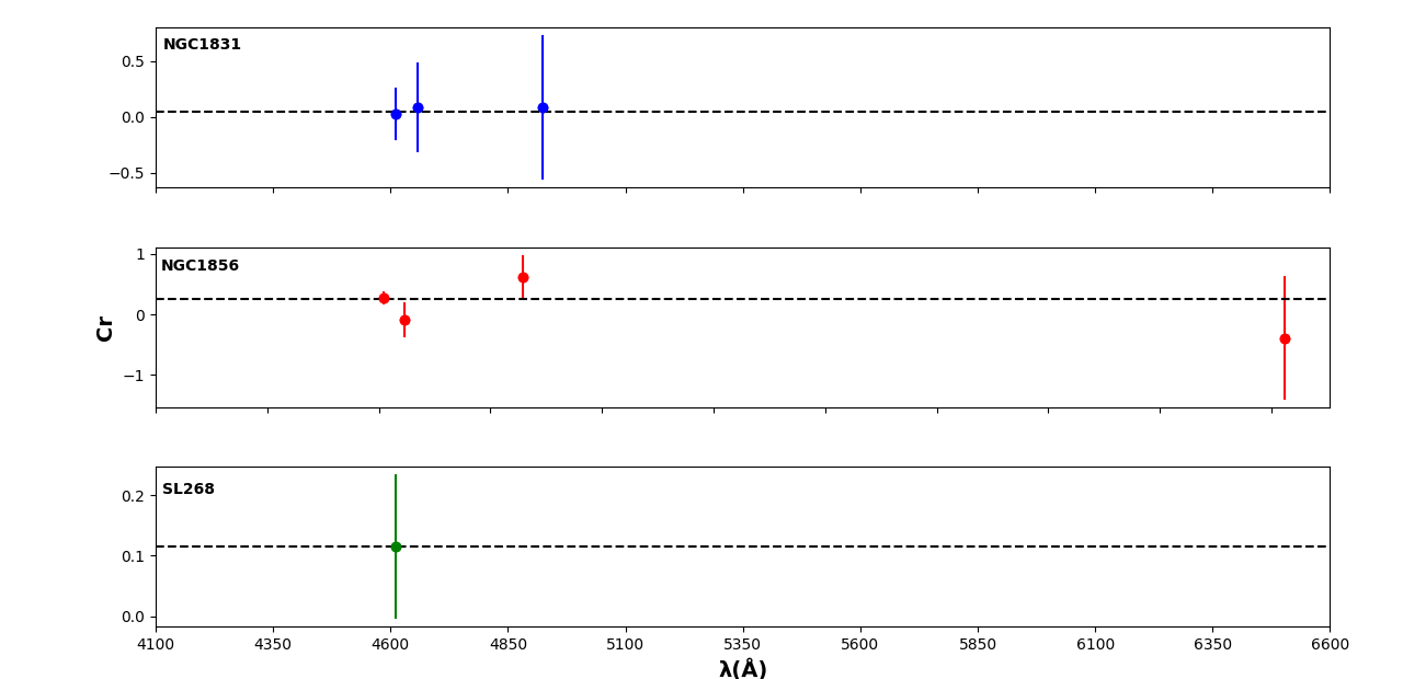
Figure 8: Cr abundances listed in Tables 3, 4 and 5 as a function of wavelength.The dotted line is the weighted average.

References

- Asa’d & Goudfrooij (2020) Asa’d, R., & Goudfrooij, P. 2020, MNRAS, 498, 2814, doi: 10.1093/mnras/staa2515
- Asa’d et al. (2021) Asa’d, R., Goudfrooij, P., As’ad, A. M., et al. 2021, MNRAS, 505, 979, doi: 10.1093/mnras/stab969
- Asa’d et al. (2020) Asa’d, R., Kovalev, M., Davies, B., et al. 2020, ApJ, 900, 138, doi: 10.3847/1538-4357/aba439
- Asa’d et al. (2016) Asa’d, R. S., Vazdekis, A., & Zeinelabdin, S. 2016, MNRAS, 457, 2151, doi: 10.1093/mnras/stw015
- Asa’d et al. (2022) Asa’d, R., Goudfrooij, P., & As’ad, A. M. 2022, Monthly Notices of the Royal Astronomical Society, doi: 10.1093/mnras/stac566
- Asplund et al. (2009) Asplund, M., Grevesse, N., Sauval, A. J., & Scott, P. 2009, ARA&A, 47, 481, doi: 10.1146/annurev.astro.46.060407.145222
- Bastian & Lardo (2018) Bastian, N., & Lardo, C. 2018, ARA&A, 56, 83, doi: 10.1146/annurev-astro-081817-051839
- Bastian et al. (2019) Bastian, N., Usher, C., Kamann, S., et al. 2019, MNRAS, 489, L80, doi: 10.1093/mnrasl/slz130
- Bastian et al. (2020) Bastian, N., Lardo, C., Usher, C., et al. 2020, MNRAS, 494, 332, doi: 10.1093/mnras/staa716
- Bradamante et al. (1998) Bradamante, F., Matteucci, F., & D’Ercole, A. 1998, A&A, 337, 338. https://arxiv.org/abs/astro-ph/9801131
- Bressan et al. (2012) Bressan, A., Marigo, P., Girardi, L., et al. 2012, MNRAS, 427, 127, doi: 10.1111/j.1365-2966.2012.21948.x
- Calura et al. (2003) Calura, F., Matteucci, F., & Vladilo, G. 2003, MNRAS, 340, 59, doi: 10.1046/j.1365-8711.2003.06197.x
- Carretta (2014) Carretta, E. 2014, ApJ, 795, L28, doi: 10.1088/2041-8205/795/2/L28
- Carretta et al. (2009) Carretta, E., Bragaglia, A., Gratton, R. G., et al. 2009, A&A, 505, 117, doi: 10.1051/0004-6361/200912096
- Castelli & Hubrig (2004) Castelli, F., & Hubrig, S. 2004, A&A, 425, 263, doi: 10.1051/0004-6361:20041011
- Chilingarian et al. (2007) Chilingarian, I., Prugniel, P., Sil’Chenko, O., & Koleva, M. 2007, in IAU Symposium, Vol. 241, Stellar Populations as Building Blocks of Galaxies, ed. A. Vazdekis & R. Peletier, 175–176