IN SEARCH OF SHORT GAMMA-RAY BURST OPTICAL COUNTERPARTS WITH THE ZWICKY TRANSIENT FACILITY

Abstract

The Fermi Gamma-ray Burst Monitor (GBM) triggers on-board in response to $\sim$ 40 short s per year; however, their large localization regions have made the search for optical counterparts a challenging endeavour. We have developed and executed an extensive program with the wide field of view of the Zwicky Transient Facility (ZTF) camera, mounted on the P48, to perform target–of–opportunity (ToO) observations on 10 Fermi-GBM SGRBs during 2018 and 2020-2021. Bridging the large sky areas with small field of view optical telescopes in order to track the evolution of potential candidates, we look for the elusive SGRB afterglows and kilonovae associated with these high-energy events. No counterpart has yet been found, even though more than 10 ground based telescopes, part of the Global Relay of Observatories Watching Transients Happen (GROWTH) network, have taken part in these efforts. The candidate selection procedure and the follow-up strategy have shown that ZTF is an efficient instrument for searching for poorly localized SGRBs, retrieving a reasonable number of candidates to follow-up and showing promising capabilities as the community approaches the multi-messenger era. Based on the median limiting magnitude of ZTF, our searches would have been able to retrieve a GW170817-like event up to $\sim$ 200  Mpc and SGRB afterglows to z = 0.16 or 0.4, depending on the assumed underlying energy model. Future ToOs will expand the horizon to z = 0.2 and 0.7 respectively.

1 Introduction

Between the years 1969–1972, the Vela Satellites discovered GRBs and further analysis confirmed their cosmic origin (Klebesadel et al., 1973). These GRBs are among the brightest events in the universe, and have been observed both in nearby galaxies as well as at cosmological distances (Metzger et al., 1997). The data collected over the years suggest a bimodal distribution in the time duration of the GRB that distinguishes two groups: long GRBs (LGRB; $T_{90}>2s$) and short GRBs (SGRB; $T_{90}<2s$) (Kouveliotou et al., 1993), where $T_{90}$ is defined as the duration that encloses the 5th to the 95th percentiles of fluence or counts, depending on the instrument.

long s have been associated with SN explosions (Bloom et al., 1999; Woosley & Bloom, 2006) and a large number of them have counterparts at longer wavelengths (Cano et al., 2017). On the other hand only $\sim 35$ SGRBs have optical/NIR detections (Fong et al., 2015; Rastinejad et al., 2021), thus their progenitors are still an active area of research. SGRBs have been shown to occur in environments with old populations of stars (Berger et al., 2005; D’Avanzo, 2015) and have long been linked with mergers of compact binaries, such as binary neutron star (BNS) and neutron star–black hole (NSBH) (Narayan et al., 1992). The discovery of the gravitational wave event GW170817  coincident with the short gamma-ray burst GRB 170817A, unambiguously confirmed BNS mergers as at least one of the mechanisms that can produce a SGRB (Abbott et al., 2017a). However, compact binary mergers might not be the only source of SGRBs, as collapsars (Ahumada et al., 2021; Zhang et al., 2021) and giant flares from magnetars (Burns et al., 2021) can masquerade as short duration GRBs. Hence, the traditional classification of a burst based solely on the time duration is subject to debate (Zhang & Choi, 2008; Bromberg et al., 2013; Amati, 2021). For example, other gamma-ray properties (i.e. the hardness ratio) can cluster the bursts in different populations (Nakar, 2007), and there are a couple of examples for which the time classification of the burst has been questioned due to the presence or lack of SN emissions (Gal-Yam et al., 2006; Ahumada et al., 2021; Zhang et al., 2021; Rossi et al., 2021). In this context, the search for the optical counterparts of SGRBs is essential to unveil the nature of their progenitors and the underlying physics.

Not all SGRBs show similar gamma-ray features and different models have tried to explain the observations. For example, the “fireball” model (Wijers et al., 1997; Mészáros & Rees, 1998) describes a highly relativistic jet of charged particle plasma emitted by a compact central engine as a result of a BNS or NSBH merger. The model predicts the production of gamma rays and hard X-rays within the jet. The interaction of the jet and the material surrounding the source produces synchrotron emission in the X-ray, optical, and radio wavelengths. This “afterglow” lasts from days to months depending on the frequency range.

Different models have been applied to the observations that followed GW170817. Among the most popular is the classical case of a narrow and highly relativistic jet powered by a compact central engine (Goldstein et al., 2017). Deviations in the light-curves derived from classical models have motivated further developments (Willingale et al., 2007; Cannizzo & Gehrels, 2009; Metzger et al., 2011; Duffell & MacFadyen, 2015), including Gaussian structured jets (Kumar & Granot, 2003; Abbott et al., 2017b; Troja et al., 2017) that can be detected off-axis and do not require the jet to point directly to Earth. Other models predict a more isotropic emission profile, produced by an expanding cocoon formed as the jet makes its way through the ejected material, reaching a Lorentz factor on the order of a few (i.e. $\Gamma\sim$ 2 to 3) (Nagakura et al., 2014; Lazzati et al., 2017; Kasliwal et al., 2017; Mooley et al., 2017).

In addition to the GRB afterglow, in the event of a BNS or NSBH merger, the highly neutron rich material undergoes rapid neutron capture ($r$-process), which creates heavy elements and enriches galaxies with rare metals (Côté et al., 2018). Some of the products of the r-process include radioactive elements; the decay of these newly created elements can energize the ejecta. The produced thermal radiation eventually powers a transient known as a kilonova (KN) (Lattimer & Schramm, 1974; Li & Paczynski, 1998; Metzger et al., 2010; Rosswog, 2015; Kasen et al., 2017). In the case of an on-axis SGRB, in most cases the optical emission is expected to be dominated by the afterglow and not by the KN. (Gompertz et al., 2018; Zhu et al., 2021). There have been attempts to separate the light of the SGRB afterglow and the KN (Fong et al., 2016; Troja et al., 2019; Ascenzi et al., 2019; O’Connor et al., 2021; Rossi et al., 2020; Fong et al., 2021), however this still presents a number of challenges.

Identifying optical counterparts to compact binary mergers can provide a rich scientific output, as demonstrated by the discovery of AT2017gfo (Chornock et al., 2017; Coulter et al., 2017; Cowperthwaite et al., 2017; Drout et al., 2017; Evans et al., 2017; Kasliwal et al., 2017; Kilpatrick et al., 2017; Lipunov et al., 2017; McCully et al., 2017; Nicholl et al., 2017; Shappee et al., 2017; Pian et al., 2017; Smartt et al., 2017) which led to discoveries in areas as diverse as $r$-process nucleosynthesis, jet physics, host galaxy properties, and even cosmology (Kasliwal et al., 2017; Arcavi et al., 2017; Tanvir et al., 2017; Chornock et al., 2017; Drout et al., 2017; Kasen et al., 2017; Pian et al., 2017; Smartt et al., 2017; Troja et al., 2017). Previous studies have used the arcminute localizations achieved with the Neil Gehrels Swift Observatory Burst Alert Telescope (BAT) to find and characterize SGRBs optical counterparts (Fong et al., 2015; Rastinejad et al., 2021), however the number of associations is still only a few dozens. Others have tried following-up thousands of square degrees of the LIGO-Virgo Collaboration (LVC) maps (Coughlin et al., 2019a, b; Andreoni et al., 2019; Goldstein et al., 2019; Andreoni et al., 2020; Hosseinzadeh et al., 2019; Vieira et al., 2020; Anand et al., 2021; Kasliwal et al., 2020) in the hopes of localizing EM counterparts to gravitational wave events, to no avail. Moreover, other studies have tried to serendipitously find the elusive KN (Chatterjee et al., 2019; Andreoni et al., 2020, 2021), but they have so far only been able to constrain the local rate of neutron star mergers using wide field of view (FOV) synoptic surveys.

In this paper we present a summary of the systematic and dedicated optical search of Fermi-GBM SGRBs using the Palomar 48-inch telescope equipped with the 47 square degree Zwicky Transient Facility camera (Graham et al., 2019; Bellm et al., 2019a) over the course of $\sim$ 2 years. Previous studies (Singer et al., 2013, 2015) have successfully found optical counterparts to GBM LGRBs using the intermediate (iPTF) (Law et al., 2009; Rau et al., 2009), and other have serendipitously found orphan afterglows and LGRBs using ZTF (Andreoni et al., 2021; Ho et al., 2022). There are ongoing projects like Global MASTER-Net (Lipunov et al., 2005), and the Gravitational-Wave Optical Transient Observe (GOTO; Mong et al. 2021) that are using optical telescopes to scan the large regions derived by GBM. We note that the optical afterglows of LGRBs are usually brighter than of SGRBs, thus the ToO strategy might differ from the one presented in this paper. We base our triggers on GBM events since GBM is more sensitive to higher energies than Swift and it detects SGRBs at four times the rate of Swift, making it the most prolific compact binary merger detector.

In section 2 we describe the facilities involved along with the observations and data taken during the campaign. We describe our filtering criteria and how candidates are selected and followed up in section 3, and detail the Fermi events we followed up in section 4. In section 5 we compare our observational limits to SGRB transients in the literature. In section 6 we discuss the implications of the optical non-detection of a source and we explore the sensitivity of our searches. Using the lightcurves of the transients generated for our efficiency analysis, we put the detection of an optical counterpart in context for future ToO follow-up efforts in section 7. We summarize our work in section 8.

2 Observations and Data

In this section we will broadly describe the characteristics of the telescopes and instruments involved in this campaign, as well as the observations. We start with the Fermi-GBM, our source of compact mergers, followed by ZTF, our optical transient discovery engine, and finally describe the facilities used for follow-up.

2.1 Fermi Gamma-ray Burst Monitor

The Gamma-ray Burst Monitor (GBM) is an instrument on board the Fermi Gamma-ray Space Telescope sensitive to gamma-ray photons with energies from 8  keV to 40  MeV (Meegan et al., 2009). The average rest frame energy peak for SGRBs ($E_{p,i}\sim 0.5$ MeV; Zhang et al. 2012) is enclosed in the observable GBM energy range and not in the Swift BAT energy range (5-150 keV). Additionally, any given burst should be seen by a number of detectors, as GBM is sensitive to gamma-rays from the entire unocculted sky.

The low local rate of Swift SGRBs has impeded the discovery of more GW170817-like transients (Dichiara et al., 2020). On the other hand, GBM detects close to 40 SGRBs per year (Meegan et al., 2009), four times the rate of Swift. However, the localization regions given by GBM usually span a large portion of the sky, going from a few hundred sq. degrees to even a few thousand square degrees. These large regions make the systematic search for counterparts technically challenging and time consuming (von Kienlin et al., 2020; Goldstein et al., 2020).

Our adopted strategy prioritizes Fermi-GBM GRB events visible from Palomar that present a hard spike, that are classified as SGRBs by the on-board GBM algorithm, and that are not detected by Swift. During the first half of our campaign (2018), we did not have any constraints on the size of the GRB localization region. However, during the second half of our campaign, we restricted our triggers to the events for which more than 75% of the error region could be covered twice in $\sim$2 hrs. With ZTF this corresponds to a requirement that 75% of the map encloses less than  500 deg²., which explains the difference in the number of triggers between the first and second half of our campaign.

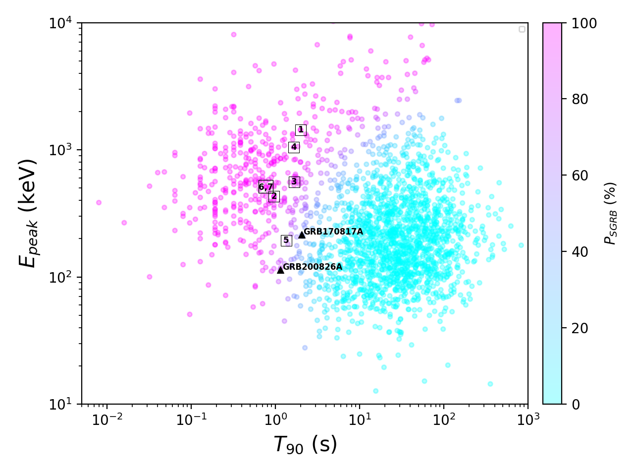
For each GRB, we calculate the probability of belonging to the population that clusters the SGRBs based on their comptonized energy peak $E_{peak}$ and their duration $T_{90}$. For this, we fit two log-normal distributions (representing the long and short classes) to a sample of   2300 GRBs. We derive and color code the probability $P_{SGRB}$ by assessing where each GRB falls in the distribution (see Fig. 1, and Ahumada et al. 2021 for more details). In Table 1 we list the relevant features of the SGRBs selected for follow-up.

Figure 1: The peak energy based on a Comptonized fit, $E_{peak}$ (keV), versus the time-integrated $T_{90}$ (s), for 2,310 Fermi GBM GRBs. The data are fit with two log-normal distributions for the two GRB classes. The colour of the data points indicates the probability, with magenta being 100% SGRB and cyan being 100% LGRB. We show in squares numbered from 1 to 7 the following SGRBs: GRB 180523B, GRB 180626C, GRB 180715B, GRB 181126B, GRB 210510A, GRB 180913A and GRB 180728B. Note that the GRB 180728B and GRB 180913A share the same location in this parameter space. The bursts GRB 200514B and GRB 201130A are not shown as the power-law model is preferred over the Comptonized fit, thus there is no $E_{peak}$ parameter associated to them. For context, we show in triangles GRB 170817A and GRB 200826A.

Table 1: Global features of the Fermi-GBM SGRB followed-up with ZTF. The peak energies come from the public Fermi catalog (von Kienlin et al., 2020) for GRB 180523B, GRB 180626C, GRB 180715B, GRB 180913A and GRB 181126B. Additionally, we compiled $E_{p}$ listed in Hamburg et al. (2018) for GRB 180728B, and independently provide time-integrated fits for GRB 200514B, GRB 201130A, and GRB 210510A over the $T_{90}$. We list the GRB name, their trigger number, the Julian day (JD) of each event, the $T_{90}$ duration, the area encompassed by the 90% (50%) credible region (C.R.), the signal-to-noise ratio from the Fermi detection, the peak energy of the gamma-ray spectrum ($E_{peak}$), the fluence of the burst, and the probability of the burst to belong to the SGRB population (see Sec. 2.1). The area associated to a given C.R. is derived by calculating the number of pixels that cumulatively sum a specific percentage, using the HEALPix map of each GRB. For events with a †, the power-law model is preferred over the comptonized model, thus there is no $E_{p}$ parameter. We show separately the parameters of GRB 200826A, as it was not related to a compact binary merger (Ahumada et al., 2021)

GRB	Fermi Trigger	Time $[$JD$]$	$T_{90}$ $[$s$]$	90% (50%) C.R. $[deg^{2}]$	S/N	$E_{peak}$ $[$keV$]$	Fluence $[10^{-8}$ erg/cm${}^{2}]$	$P_{SGRB}$
GRB 180523B	548793993	2458262.2823	2.0 $\pm$ 1.4	5094 (852)	6.9	$1434\pm 443$	25.7$\pm$ 2.3	0.99
GRB 180626C	551697835	2458295.8916	1.0 $\pm$ 0.4	5509 (349)	7.1	$431\pm 81$	49.1 $\pm$ 3.8	0.97
GRB 180715B	553369644	2458315.2412	1.7 $\pm$ 1.4	4383 (192)	12.5	$560\pm 89$	52.0 $\pm$ 1.7	0.92
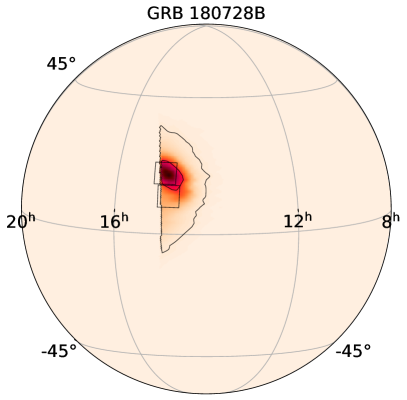
GRB 180728B	554505003	2458328.3819	0.8 $\pm$ 0.6	397 (47)	20.2	$504\pm 61$	130.9 $\pm$ 2.0	0.99
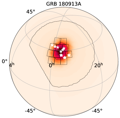
GRB 180913A	558557292	2458375.2834	0.8 $\pm$ 0.1	3951 (216)	10.0	$508\pm 90$	79.1 $\pm$ 2.0	0.99
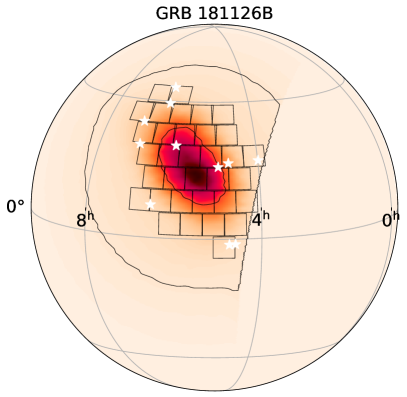
GRB 181126B	564897175	2458448.6617	1.7 $\pm$ 0.5	3785 (356)	7.5	$1049\pm 241$	48.3 $\pm$ 3.2	0.99
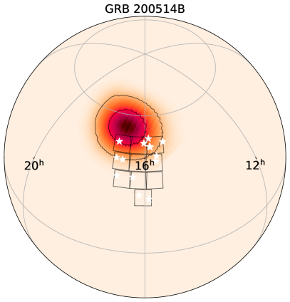
GRB 200514B	611140062	2458983.8802	1.7 $\pm$ 0.6	590 (173)	5.1	†	17.8 $\pm$ 1.1	–
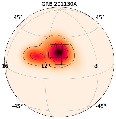
GRB 201130A	628407054	2459183.7297	1.3 $\pm$ 0.8	545 (139)	5.3	†	37.0 $\pm$ 5.2	–
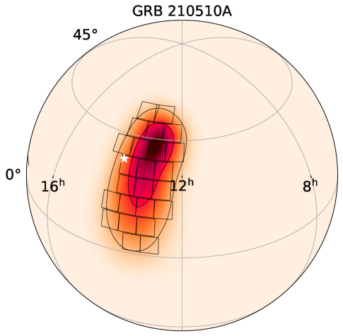
GRB 210510A	642367205	2459345.3055	1.3 $\pm$ 0.8	1170 (343)	5.6	$194\pm 60$	23.2 $\pm$ 1.4	0.74
GRB 200826A	620108997	2459087.6874	1.1 $\pm$ 0.1	339 (63)	8.1	$88.9\pm 3.2$	426.5 $\pm$ 2.2	0.74

2.2 The Zwicky Transient Facility

We have used ZTF to scan the localization regions derived by the Fermi-GBM. ZTF is a public-private project in the time domain realm which employs a dedicated camera (Dekany et al., 2020) on the Palomar 48-inch Schmidt telescope. The ZTF field of view is 47 deg², which usually allows us to observe more than 50% of the SGRB error region in less than one night. The public ZTF survey (Bellm et al., 2019b) covers the observable northern sky every two nights in $g$- and $r$-bands with a standard exposure time of 30 s, reaching an average $5\sigma$ detection limit of $r=20.6$.

Two ToO strategies were tested during this campaign, one during 2018 and the second during 2020-2021. Most modifications came after lessons learned during the follow-up efforts of gravitational waves in 2019 (Coughlin et al., 2019b; Anand et al., 2021; Kasliwal et al., 2020). The original ToO observing plan allowed us to start up to 36 hrs from the SGRB GBM trigger. However, since the afterglow we expect is already faint ($m_{r}>19$ mag) and fast fading ($\Delta m/\Delta t>0.3$ mag per day), our revised strategy only includes triggers that can be observed from Palomar within 12 hrs. The exposure time for each trigger ranges from 60 s to 300 s depending on the size of the localization region, as there is a trade-off between exposure time and coverage. We generally prioritized coverage over depth, and for the second half of our campaign, we only triggered on maps where more than 75% of the region could be covered. The same sequence is repeated a second time the following night, unless additional information from other spacecraft modifies the error region. Generally, fields with an airmass $>$ 2.5 are removed from the observing plan.

We schedule two to three sets of observations depending on the visibility of the region, using the ZTF $r$- and $g$-bands. The combination of $r$- and $g$-band observations was motivated by the need to look for afterglows and KNe, which are both fast evolving red transients. In fact, the SGRB afterglows in the literature show red colors (i.e. $g-r>0.3$ mag) and a rapid evolution, fading faster than $\Delta m_{r}/\Delta t>0.5$ mag per day. On the other hand, GW170817 started off with bluer colors and evolved dramatically fast in the optical during the first days, with $g-r=0.5$ mag  1 day after the Fermi alert and $\Delta m_{g}/\Delta t>1$ mag per day. Even though we expect a fast fading transient, if we assume conservative fading rates of 0.3-0.5 mag per day, we would need observations separated by 8 to 5 hrs respectively to detect the decline using ZTF data with photometric errors of the order of 0.1 mag. This ToO strategy thus relies on the color of transients for candidate discrimination, as this is easier to schedule than multi-epoch single-band photometry within the same night and with sufficient spacing between observations.

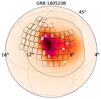
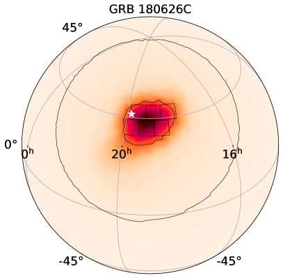
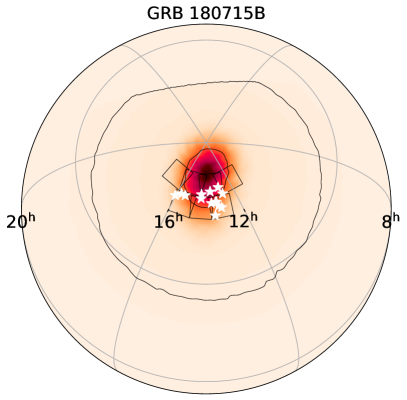
We followed up on 10 Fermi-GBM SGRBs, and we show 9 skymaps and their corresponding ZTF footprints in Fig. 2, 3, and 4. Please refer to Ahumada et al. 2021 for details on GRB 200826A, the only short duration GRB followed up during our campaign that is not shown here. As listed in Table 1, all of the events span more than 100  deg², which is the average localization region covered during previous LGRBs searches (Singer et al., 2015). Moreover, in many cases, the 90% credible region (C.R.) spans more than 1000  deg², which is challenging even for a 47  deg² field of view instrument such as ZTF.

Triggering ToO observations for survey instruments like ZTF and Palomar Gattini-IR (De et al., 2020) halts their ongoing survey observations and redirects them to observe only certain fields as directed by an observation plan. We have used gwemopt (Coughlin et al., 2018, 2019a), a code intended to optimize targeted observations for gravitational wave events, to achieve an efficient schedule for our ToO observations. The similarities between LVC and GBM skymaps allow us to apply the same algorithm, which involves slicing the skymap into the predefined ZTF tiles and determining the optimal schedule by taking into consideration the observability windows and the need for a repeated exposure of the fields. In order to prioritize the fields with the highest enclosed probability, we used the “greedy” algorithm described in Coughlin et al. (2018) and Almualla et al. (2020). As gwemopt handles both synoptic and galaxy-targeted search strategies, we employed the former to conduct observations with some of our facilities, Palomar Gattini-IR, GROWTH-India and ZTF, and the latter for scheduling observations with the Kitt Peak EMCCD Demonstrator (KPED; Coughlin et al. 2019b).

Figure 2: Coverage of four ZTF triggers and their Fermi GBM localization regions. Starting on the top left, the skymaps of GRB 180523, GRB 180626, GRB 180715, and GRB 180728 are shown along the $\approx$ 47 deg² ZTF tiles (black quadrilaterals). The 50% and 90% credible regions are shown as black contours and the sources discovered during the ZTF trigger as white stars (details in Section 4). The grid shows the Right Ascension in hours and the Declination in degrees.

Figure 3: Coverage of four ZTF triggers and their Fermi GBM localization regions. From top to bottom and left to right, the skymaps of GRB 180913, GRB 181126, GRB 200514, and GRB 201130 are shown along the $\approx$ 47 deg² ZTF tiles (black quadrilaterals). The 50% and 90% credible regions are shown as black contours and the sources discovered during the ZTF trigger as white stars (details in Section 4). Note that for GRB 200514, we tiled the preliminary region, which was offset from the final localization. The grid shows the Right Ascension in hours and the Declination in degrees.

Figure 4: Coverage of the ZTF trigger and Fermi GBM localization region of GRB 210510, along the $\approx$ 47 deg² ZTF tiles (black quadrilaterals). The 50% and 90% credible regions are shown as black contours and the source discovered during the ZTF trigger as white star (details in Section 4). The grid shows the Right Ascension in hours and the Declination in degrees.

2.3 Optical follow-up

Following the identification of candidate counterparts with ZTF, subsequent optical follow-up of these transients is required to characterize and classify them. For the candidates that met the requirements described in section 3, mainly that they showed interesting light-curve history and magnitude evolution, we acquired additional data. To obtain these data, the GROWTH multi-messenger group relies on a number of telescopes around the globe. Most of these facilities are strategically located in the Northern Hemisphere, enabling continuous follow-up of ZTF sources. The follow-up observations included both photometric and spectroscopic observations. Even though the spectroscopic classification is preferable, photometry was essential to rule out transients, based on their color evolution and fading rates. The telescopes involved in the photometric and spectroscopic monitoring are briefly described in the following paragraphs.

We used the Kitt Peak Electron multiplying CCD Demonstrator (KPED) on the Kitt Peak 84 inch telescope (Coughlin et al., 2019b) to obtain photometric data. The KPED is an instrument mounted on a fully robotic telescope and it has been used as a single-band optical detector in the Sloan $g-$ and $r-$ bands and Johnson UVRI filters. The FOV is 4.4^′ $\times$ 4.4^′ and the pixel size is 0.259^′′.

Each candidate scheduled for photometry was observed in the $g$- and $r$- band for 300 s. The data taken with KPED are then dark subtracted and flat-field calibrated. After applying astrometric corrections, the instrumental magnitudes were determined using Source Extractor (Bertin & Arnouts, 1996). To calculate the apparent magnitude of the candidate, the zero-point of the field is calibrated using Pan–STARRS 1 (PS1) and Sloan Digital Sky Survey (SDSS) stars in the field as standards. Given the coordinates of the target, an on-the-fly query to PAN-STARRS1 and SDSS retrieves the stars within the field that have a minimum of 4 detections in each band.

Additionally, sources were photometrically followed-up using the Las Cumbres Observatory Global Telescope (LCOGT) (PI: Coughlin, Andreoni) (Brown et al., 2013). We used the 1-m and 2-m telescopes to schedule sets of 300 s in the $g$-, $r$- and $i$-band. The LCOGT data come already processed and in order to determine the magnitude of the transient, the same PS1/SDSS crossmatching strategy used for KPED was implemented for LCOGT images.

We used the Spectral Energy Distribution Machine (SEDM) on the Palomar 60-inch telescope (Blagorodnova et al., 2018) to acquire $g$-, $r$-, and $i$- band imaging with the Rainbow Camera on SEDM in 300 s exposures. Images were then processed using a python-based pipeline that performs standard photometric reduction techniques and uses an adaptation of FPipe (Fremling Automated Pipeline; described in detail in Fremling et al. 2016) for difference imaging. Moreover, we employed the Integral Field Unit (IFU) on SEDM to observe targets brighter than m${}_{AB}<19$ mag. Each observation is reduced and calibrated using the pysedm pipeline (Rigault et al., 2019), which applies standard calibrations using standards taken during the observing night. Once the spectra are extracted we use the SuperNova IDentification software (SNID; Blondin & Tonry, 2007) for spectroscopic classification.

We obtained spectra for six candidates using the Double Spectrograph (DBSP) on the Palomar 200-inch telescope during classical observing runs. The data were taken using the 1.5″slit and reduced following a custom PyRAF pipeline (Bellm & Sesar, 2016).

The other telescopes used for photometric follow-up are the GROWTH India telescope (GIT) in Hanle, India, the Liverpool Telescope (Steele et al., 2004) in La Palma, Spain, and the Akeno telescope (Kotani et al., 2005) in Japan. The requested observations in the $g$-, $r$- and $i$-band varied between 300s  and 600s  depending on the telescope.

We obtained spectra with the DeVeny Spectrograph at the Lowell Discovery Telescope (LDT) (MacFarlane & Dunham, 2004) and the 10m Keck Low Resolution Imaging Spectrograph (LRIS) (Oke et al., 1995). We reduced these spectra with PyRAF following standard long-slit reduction methods.

We used the Gemini Multi-Object Spectrograph (GMOS-N) mounted on the Gemini-North 8-meter telescope on Mauna Kea to obtain photometric and spectroscopic data (P.I. Ahumada, GN-2021A-Q-102). Our standard photometric epochs consisted of four 180s exposures in $r$-band to measure the fading rate of the candidates, although we included $g$-band when the color was relevant. These images were processed using DRAGONS (Labrie et al., 2019) and the magnitudes were derived after calibrating against PS1. When necessary and possible, we used PS1 references to subtract the host, using HOTPANTS. For spectroscopic data, our standard was four 650 s exposures using the 1″long-slit and the R400 grating and we used PyRAF standard reduction techniques to reduce the data.

3 Candidates

After a given ZTF observation finishes, the resulting image is subtracted to a reference image of the field (Masci et al., 2019; Zackay et al., 2016). The latter process involves a refined PSF adjustment and a precise image alignment in order to perform the subtraction and determine flux residuals. Any $5\sigma$ difference in brightness creates an ‘alert’ (Patterson et al., 2019), a package with information describing the transient. The alerts include the magnitude of the transient, proximity to other sources and its previous history of detections among other features. ZTF generates around $10^{5}$ alerts per night of observation, which corresponds to $\sim 10\%$ of the estimated Vera Rubin observatory alert rate. The procedure to reduce the number of alerts from $\sim 10^{5}$ to a handful of potential optical SGRB counterparts is described in this section.

In general terms, the method involves a rigid online alert filtering scheme that significantly reduces the number of sources based on image quality features. Then, the selection of candidates takes into consideration the physical properties of the transient (i.e. cross-matching with AGN and solar system objects), as well as archival observations from different surveys. After visually inspecting the candidates that passed the preliminary filters, scientists in the collaboration proceed to select sources based on their light-curves, color and other features (i.e. proximity to a potential host, redshift of the host, etc.). This method allows us to recover objects that are later scheduled for further follow-up.

The candidate selection and the follow-up are coordinated via the GROWTH marshal (Kasliwal et al., 2019) and lately through the open-source platform and alert broker Fritz.

3.1 Detection and filtering

In the searches for the optical counterpart for SGRBs, we query the ZTF data stream using the GROWTH marshal (Kasliwal et al., 2019), the Kowalski infrastructure (Duev et al., 2019), the NuZTF pipeline (Stein et al., 2021, 2021) built using Ampel (Nordin et al., 2019) , and Fritz. The filtering scheme restricted the transients to those with the following properties:

• Within the skymap: To ensure the candidates are in the GBM skymap, we implemented a cone search in the GBM region with Kowalski and Ampel. With the GROWTH marshal approach, we retrieve only the candidates in the fields scheduled for ToO. We note that a more refined analysis on the coordinates of the candidates is done after this automatic selection.

• Positive subtraction: After the new image is subtracted, we filter on the sources with a positive residual, thus the ones that have brightened.

• It is real: To distinguish sources that are created by ghosts or artifacts in the CCDs, we apply a random-forest model (Mahabal et al., 2019) that was trained with common artifacts found in the ZTF images. We restrict the Real-Bogus score to $>0.25$ as it best separates the two populations. For observations that occurred after 2019, we used the improved deep learning real-bogus score drb and we set the threshold to sources with drb score $>0.15$ (Duev et al., 2019).

• No point source underneath: To rule out stellar variability we require the transient to have a separation of 3″  from any point source in the PS1 catalog based on Tachibana & Miller (2018).

• Two detections: We require a minimum of two detections separated by at least 30 min. This allows us to reject cosmic rays and moving solar system objects.

• Far from a bright star: To further avoid ghosts and artifacts, we require the transient to be $>$ 20″  from any bright ($m_{\textrm{AB}}<15$ mag) star.

• No previous history: As we do not expect the optical counterpart of a SGRB to be a periodic variable source, we restrict our selection to only sources that are detected after the event time and have no alerts generated for dates prior to the GRB.

As a reference, this first filtering step reduced the total number of sources to a median of $\sim 0.03\%$ of the original number of alerts. The breakdown of each filter step is shown in Table 2. A summary of the numbers of followed-up objects for each trigger is in Table 3 and the details of the filtering scheme are described below. More than 3 $\times 10^{5}$ alerts were generated during the 9 ToO triggers, while $\sim$80 objects were circulated in the Gamma-ray Coordinates Network (GCN).

Table 2: Summary of the efficiency of our vetting strategy. For each GRB we list the number of alerts that survives after a given filtering step. The first column (SNR$>$5) shows the total number of alerts in the GRB map. The next column displays the number of alerts that show an increase in flux (Positive subtraction). The ’Real‘ column shows the number of sources considered as real using either the real-bogus index(RB) or drb scores. We set the thresholds to RB$>$0.25 and drb$>$0.5. The next columns show the number of sources that are not related to a point source, nor close to a bright star, to avoid artifacts. To avoid moving objects, we show the number of sources with two detections separated by at least 30 min. The last column shows the number of sources we circulated as potential candidates for each trigger. For each step, we calculate the median reduction of alerts and list this number at the end of each column.

GRB	SNR$>$5	Positive subtraction	Real	Not star underneath	Far from bright star	Two detections	Circulated in GCNs
GRB 180523B	67614	17374	12117	687	669	297	14
GRB 180626C	10602	5040	4967	1582	1377	214	1
GRB 180715B	33064	7611	7515	6941	5509	104	14
GRB 180728B	18488	1450	1428	859	739	51	7
GRB 180913A	25913	12105	12077	6284	5145	372	12
GRB 181126B	40342	30455	30416	22759	21769	340	11
GRB 200514B	20610	10983	10602	4502	4422	1346	14
GRB 200826A	13488	8142	7744	3892	3785	464	14
GRB 201130A	1972	1045	990	647	637	43	0
GRB 210510A	41683	27229	28940	16977	16973	1562	1
Median reduction		50.27%	48.53%	23.05 %	20.66%	1.73%	0.03%

3.2 Scanning and selection

Generally, after the first filter step, the number of transients is reduced to a manageable amount $\sim O(100)$. These candidates are then cross-matched with public all-sky surveys such as Wide-field Infrared Survey Explorer (WISE; Cutri et al., 2013), Pan–STARRS 1 (PS1; Chambers et al., 2016), Sloan Digital Sky Survey (SDSS; Ahumada et al., 2020a), the Catalina Real-time Transient Survey (CRTS; Drake et al., 2009), and the Asteroid Terrestrial-impact Last Alert System (ATLAS; Tonry, 2011). We use the Wide-field Infrared Survey Explorer (WISE) colors to rule out candidates, as active galactic nuclei are located in a particular region in the WISE color space (Wright et al., 2010; Stern et al., 2012). If a candidate has a previous detection in Asteroid Terrestrial-impact Last Alert System (ATLAS) or has been reported to the Transient Name Server (TNS) before the event time it is also removed from the candidate list. We additionally crossmatch the position of the candidates with the Minor Planet Center (MPC) to rule out any other slow moving object. We use the PS1 DR2 to query single detections at the location of the transients, and we use this information to rule out sources based on serendipitous previous activity.

One of the most important steps in our selection of transients is the rejection of sources using forced photometry (FP) on ZTF images. For this purpose we run two FP pipelines: ForcePhotZTF (Yao et al., 2019) and the ZTF FP pipeline (Masci et al., 2019). We limit our search to 100 days before the burst and reject sources with consistent $\geq$ 4$\sigma$ detections.

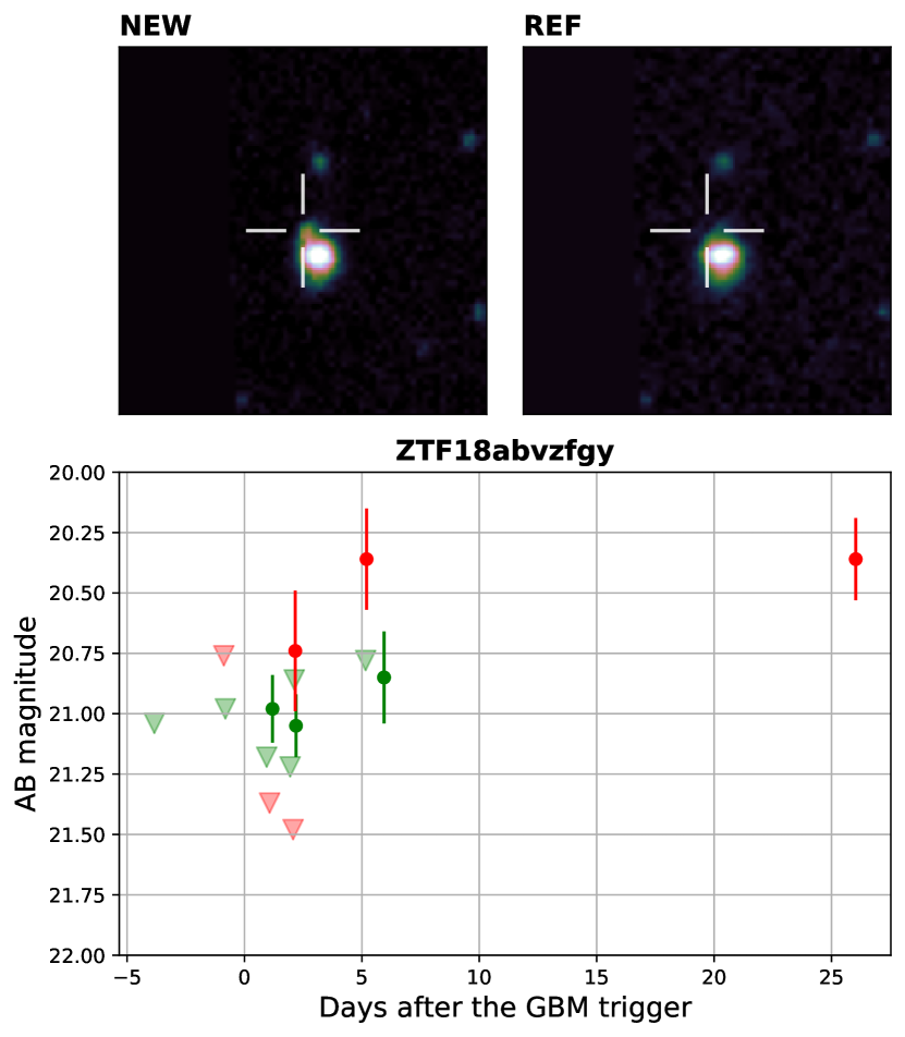
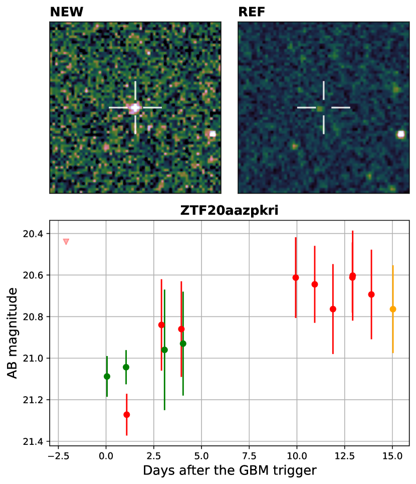
Finally, we manually scan and vet candidates passing those cuts, referring to cutouts of the science images, photometric decay rates, and color evolution information in order to select the most promising candidates (see Fig. 5).

Detailed tables with the candidates discovered by ZTF for the SGRB campaign are shown in Table 4

Figure 5: Examples of light-curves and cut-outs for candidates that passed our filtering criteria. Candidate ZTF18abvzfgy (candidate counterpart to GRB 180913A) in the left panel and ZTF20aazpkri (candidate counterpart to GRB 200514B) in the right panel. The observations in $g-$ and $r-$ band are plotted in green and red colors respectively. Filled circles represent ZTF detections, while the 5$\sigma$ upper limits are shown as triangles in the light-curve. The top half of each panel shows the discovery image on the left and the reference image on the right. In the 0.7 sq. arcmin cutouts, north is up and east is to the left. A cross marks the location of the transient.

3.3 Rejection Criteria

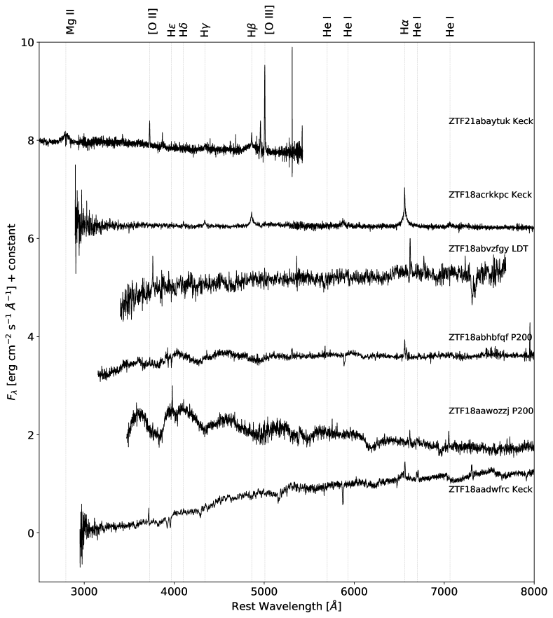
In order to find an optical counterpart, further monitoring of the discovered transients is needed. We have taken spectra for the most promising candidates to classify them. Most of the spectra acquired correspond to bright SNe (as in Fig. 6) and a few Cataclysmic Variables and an AGN. After the 9 SGRBs follow-ups, we obtained 19 spectra, however none of them exhibited KN features. We have used the ‘Deep Learning for the Automated Spectral Classification of Supernovae and Their Hosts’ or dash (Muthukrishna et al., 2019) to determine the classification of the candidates with SN spectral features. CVs were recognized as they show H features at redshift $z$ = 0.

For the sources that do not have spectra available, we monitored their photometric evolution with the facilities described in Section 2. Even though the photometric classification cannot be entirely conclusive, there are characteristic features shared between afterglows and KNe. On one side, afterglows are known to follow a power-law decay of the form $F\sim t^{-\alpha}$. On the other hand, most KN models (Bulla, 2019) show evolution faster than 0.3 mag per day (Anand et al. 2021; Andreoni et al. 2020). As a reference, GW170817 faded over $\sim$ 1  mag over the course of 3  days and other SGRB optical counterparts have shown a rapid magnitude evolution as well (Fong et al., 2015; Rastinejad et al., 2021). The astrophysical events that most contaminated our sample are SNe, but they normally show a monotonic increase in their brightness during their first tens of days, to later decline at a slower rate than expected for afterglows or KNe. Other objects like slow-moving asteroids and flares are less common and can be removed inspecting the images or performing a detailed archival search in ZTF and other surveys.

To illustrate the photometric rejection, we show two transients in Fig. 5 with no previous activity in the ZTF archives previous to the SGRB. As their magnitude evolution in both $r-$ and $g-$ band does not pass our threshold, we conclude that they are not related to the event. This process was repeated for all candidates without spectral information, using all the available photometric data from ZTF and partner telescopes.

4 SGRB events

4.1 GRB 180523B

The first set of ToO observations of this program was taken 9.1 hours after GRB 180523B (trigger 548793993). We covered $\sim$ 2900  deg², which corresponds to 60% of the localization region after accounting for chip gaps in the instrument (Coughlin et al., 2018b). The median 5$\sigma$ upper limit for an isolated point source in our images was r $>$ 20.3 mag and g $>$ 20.6  mag and after 2  days of observations we arrived at 14 viable candidates that required follow-up. We were able to spectroscopically classify 4 transients as SNe and photometrically follow-up sources with KPED to determine that the magnitude evolution was slower than our threshold. This effort was summarized in Coughlin et al. (2019a) and the list of transients discovered is displayed in Table 4.

4.2 GRB 180626C

The SGRB GRB 180626C (Fermi trigger 551697835) came in the middle of the night at Palomar. We started observing after 1.5  hours and were able to cover 275 deg² of the GBM region. The localization, and hence the observing plan, was later updated as the region of interest was now the overlap between the Fermi and the newly arrived InterPlanetary Network (IPN) map. The observations covered finally 230 deg², corresponding to 87% of the intersecting region. After two nights of observations, with a median 5-sigma upper limit of r $>$ 21.1 mag and g $>$ 21.0 mag, only one candidate was found to have no previous history of evolution and be spatially coincident with the SGRB (Coughlin et al., 2018a).

The transient ZTF18aauebur was a rapidly evolving transient that faded from g = 18.4 to g = 20.5 in 1.92 days. This rapid evolution continued during the following months, fluctuating between r $\sim$ 18 mag and r $\sim$ 19 mag. It was interpreted as a stellar flare, as it is located close to the Galactic plane and there is an underlying source in the PS1 and Galaxy Evolution Explorer (GALEX) (Morrissey et al., 2007) archive. Additionally, its SEDM spectrum showed a featureless blue spectrum and H$\alpha$ absorption features at redshift z = 0, so it is an unrelated Galactic source. The rest of the candidates can be found in Table 4.

4.3 GRB 180715B

We triggered ToO observations to follow-up GRB 180715B (trigger 553369644) 10.3  hours after the GBM detection. We managed to observe $\sim$ 36% of the localization region which translates into 254 deg². The median limiting magnitude for these observations was r $>$ 21.4 mag and g $>$ 21.3 mag.

During this campaign, we discovered 14 new transients (Cenko et al., 2018) in the region of interest. We were able to spectroscopically classify 2 candidates using instruments at the robotic Palomar 60 inch telescope (P60) and Palomar 200 inch Hale telescope (P200). The SEDM spectrum of ZTF18aauhpyb showed a stellar source with Balmer features at redshift z = 0 and a blue continuum. The DBSP spectrum of ZTF18abhbfqf was best fitted by a SN Ia-91T. We show the rejection criteria used to rule-out associations with the SGRB in Table 4. Generally, most candidates showed a slow magnitude evolution. Furthermore, three candidates (ZTF18abhhjyd, ZTF18abhbfoi and ZTF18abhawjn) matched with an AGN in the Milliquas (Flesch, 2019) catalog. A summary of the candidates can be found in Table 4.

4.4 GRB 180728B

The ToO observations of GRB 180728B (trigger 554505003) started $\sim$ 8  hours after the Fermi alert, however, it did not cover the later updated IPN localization. The following night and 31  hours after the Fermi detection we managed to observe the joint GBM and IPN localization, covering 334 deg² which is $\sim$ 76% of the error region. The median upper limits for the scheduled observations were r $>$ 18.7 mag and g $>$ 20.0 mag (Coughlin et al., 2018a). As a result of these observations, no new transients were found.

4.5 GRB 180913A

We triggered ToO observations with ZTF to follow-up the Fermi event GRB 180913A (trigger 558557292) about $\sim$ 8  hours after the GBM detection. The first night of observations covered 546  deg². The schedule was adjusted as the localization improved once the IPN map was available. During the second night we covered 53% of the localization, translated into 403  deg². After a third night of observations, 12 transients were discovered and circulated in Coughlin et al. (2018b). The median upper limits for this set of observations were r $>$ 21.9 and g $>$ 22.1 mag.

We obtained a spectrum of ZTF18abvzfgy with LDT, a fast rising transient ($\Delta m/\Delta t\sim-0.2$ mag per day) in the outskirts of a potential host galaxy. It was classified as a SN Ic at a redshift of z = 0.04. The rest of the transients were follow-up photometrically with KPED and LCO, but generally showed a flat evolution. The candidate ZTF18abvzsld had previous PS1 detections, thus ruling it out as a SGRB counterpart. The rest of the candidates are listed in Table 4.

4.6 GRB 181126B

The last SGRB we followed-up before the start of the 2019 O3 LIGO/Virgo observing run was of the Fermi-GBM event GRB 181126B (trigger 564897175). As this event came during the night at the ZTF site, the observations started $\sim$ 1.3  hours after the Fermi alert, and we were able to cover 1400  deg², close to 66% of the GBM localization. After the IPN localization was available the next day, the observations were adjusted and we used ZTF to cover 709 deg², or $\sim$ 76% of the overlapped region. The mean limiting magnitude of the observations was r $>$ 20.8 mag (Ahumada et al., 2018). After processing the data, we discovered 11 new optical transients timely and spatially coincident with the SGRB event. We took spectra of 7 of them with the Keck LRIS, discovering 6 SNe (ZTF18acrkkpc, ZTF18aadwfrc, ZTF18acrfond, ZTF18acrfymv, ZTF18acptgzz, ZTF18acrewzd) and 1 stellar flare (ZTF18acrkcxa). All of the candidates are listed in Table 4, and none of them showed rapid evolution.

4.7 GRB 200514B

We resumed the search for SGRB counterparts with ZTF once LIGO/Virgo finished O3. On 2020-05-14 we used ZTF to cover over 519.3 deg² of the error region of GRB 200514B (trigger 611140062). This corresponds to $\sim 50\%$ of the error region. After the first night of observations, 7 candidates passed our filters and were later circulated in Ahumada et al. (2020). The observations during the following night resulted in 7 additional candidates (Reusch et al., 2020a). The depth of these observations reached 22.4 and 22.2 mag in the $g-$ and $r-$band respectively. After IPN released their analysis (Svinkin et al., 2020), 9 of our candidates remained in the localization region. Our follow-up with ZTF and LCO showed that none of these transients evolved as fast as expected for a GRB afterglow (see Table 4).

4.8 GRB 200826A

This burst is discussed extensively in Ahumada et al. (2021), as well as in other works (Zhang et al., 2021; Rossi et al., 2021; Rhodes et al., 2021). It was the only short duration GRB in our campaign with an optical counterpart association. However, despite its short duration ($T_{90}$ = 1.13s), it showed a photometric bump in the $i$-band that could only be explained by an underlying SN (Ahumada et al., 2020b, c). This makes GRB 200826A the shortest-duration LGRB Ahumada et al. (2021).

4.9 GRB 201130A

The ZTF trigger on GRB 201130A reached a depth of r = 20.5 mag in the first night of observations after covering 75% of the credible region. No optical transient passed all our filtering criteria (Reusch et al., 2020b).

4.10 GRB 210510A

We triggered optical observations on GRB 210510A (trigger 642367205) roughly 10 hrs after the burst. The second night of observations helped with vetting candidates based on their photometric evolution, at least a 0.3 mag per day decay rate is expected for afterglows and KNe. The only candidate that passed our filtering criteria was ZTF21abaytuk (Anand et al., 2021), however its Keck LRIS spectrum showed H$\beta$, [O II], and [O III] emission features and Mg II absorption lines at redshift of z = 0.89 (see Table 4 and Fig. 6). Its spectrum, summed with its WISE colors, are consistent with an AGN origin.

Figure 6: The spectra of some representative candidates. The spectrum of transient ZTF18aadwfrc was taken with the LRIS at the Keck Observatory and was classified as a SN Ia at z = 0.04. Similarly, the spectrum of ZTF18acrkkpc and ZTF21abaytuk come from Keck as well, and were classified as a SN II at z = 0.061 and as an AGN at z = 0.89 respectively. We used the DBSP at P200 to aqcuire spectra of ZTF18aawozzj and ZTF18abhbfqf, two SN Ia at redshift z = 0.095 and z= 0.11 respectively. Lastly, the spectrum of ZTF18abvzfgy was obtained with the DeVeny Spectrograph at the LDT, and using dash, we classified it as a SN Ic at z = 0.04. For reference, we show the Hydrogen, Helium, Magnesium, and some Oxygen lines as vertical lines.

5 ZTF upper limits

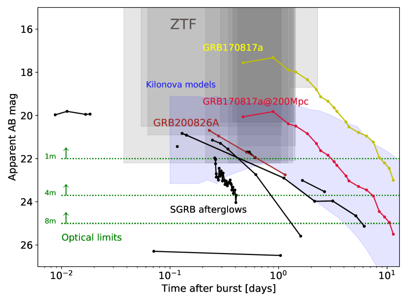
It is possible to compare the search sensitivity, both in terms of depth and timescale, to the expected afterglow and kilonova light-curves. In the left panel of Fig. 7, the median limits for ZTF observations are shown with respect to known Swift SGRB afterglows with measured redshift from Fong et al. (2015). The yellow light-curve corresponds to GW170817 (Abbott et al., 2017c) and the red line is the same GW170817  light-curve scaled to a distance of 200  Mpc (see below). Along with GW170817, we show a collection of KN light-curves from a BNS grid (Bulla, 2019; Dietrich et al., 2020) scaled to 200 Mpc. The regions of the light-curve space explored by each ZTF trigger are represented as grey rectangles and the more opaque region corresponds to their intersection. Even though ZTF has the ability to detect a GW170817-like event and most of the KN lightcurves, most of the SGRB afterglows observed in the past are below the median sensitivity of the telescope. On the other hand, the counterpart of the GRB 200826A would have been detected in six of our searches, even though it is on the less energetic part of the LGRB distribution. When scaled to 200 Mpc, the GW170817  light-curve overlaps with the region of five of our searches, suggesting that the combination of depth and rapid coverage of the regions could allow us to detect an GW170817-like event. The searches that do not overlap with the scaled GW170817  have either fainter median magnitude upper limits ($<20$ mag) or late starting times ($>1$ day).

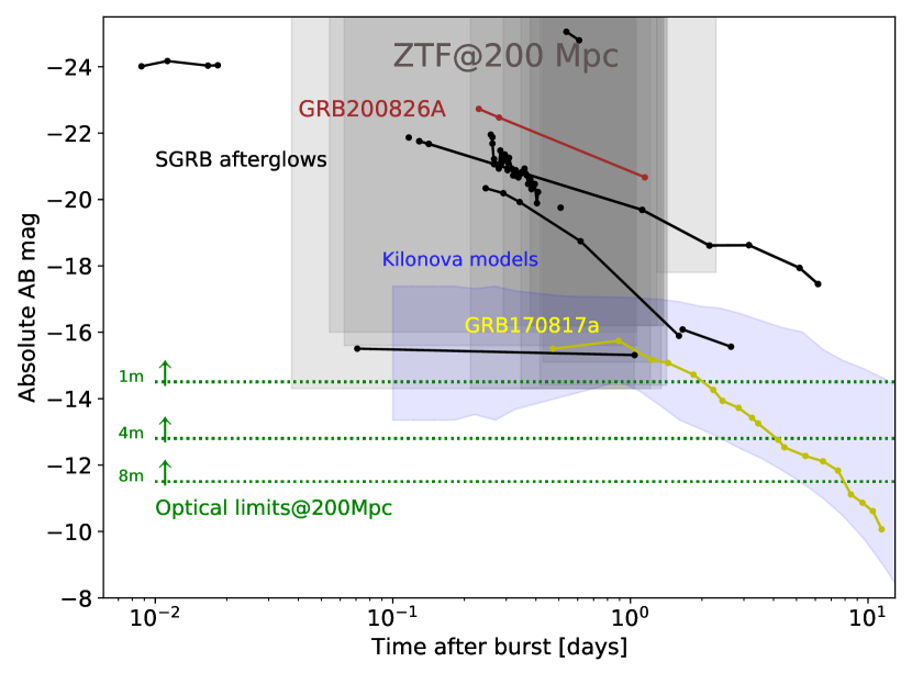
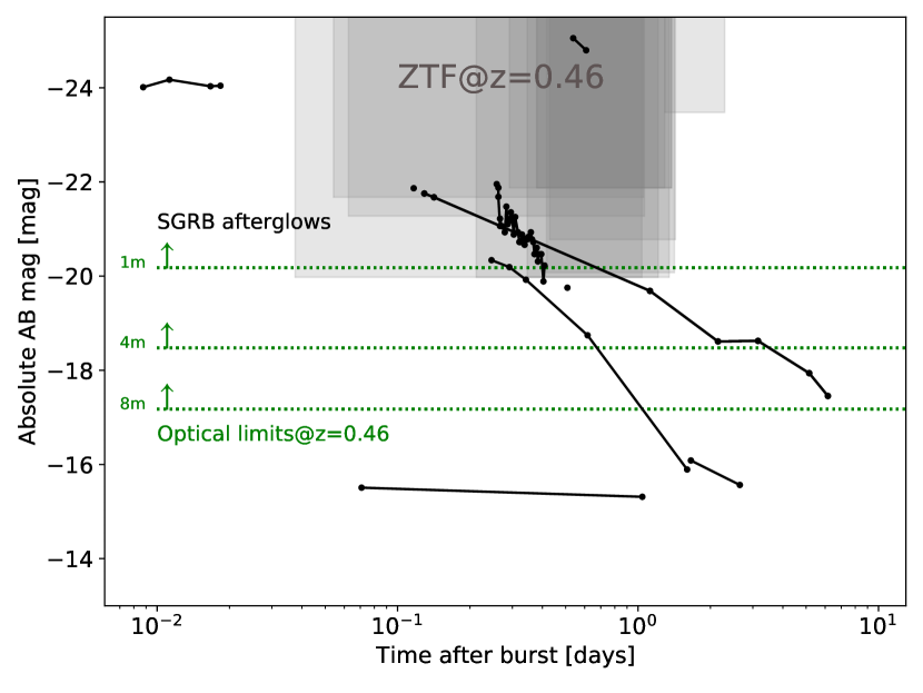
We used the redshifts of the SGRBs optical counterparts to determine their absolute magnitudes, which is plotted in the right panel in Fig. 7, along with GRB 200826A and GW170817. In order to compare with the ZTF searches and constrain the observations, the median ZTF limits were scaled to a fiducial distance of 200 Mpc, the O3 LIGO/Virgo detection horizon (Abbott et al., 2018) for binary neutron star (BNS) mergers. The range of 200 Mpc is coincidentally approximately the furthest distance as to which ZTF can detect a GW170817-like event based on the median limiting magnitudes of this experiment. Moreover, the ZTF region covers most of the KNe models (blue shaded region) scaled to 200 Mpc. In contrast to the left panel in Fig. 7, most of the SGRB optical afterglows fall in the region explored by ZTF. Therefore, if any similar events happened within 200 Mpc, the current ZTF ToO depth plus a rapid trigger of the observations should suffice to ensure coverage in the light-curve space. Previous studies (Dichiara et al., 2020) have come to the conclusion that the low rate of local SGRB is responsible for the lack of detection GW170817-like transients. In fact, the probability that one of the SGRBs in our sample is within 200 Mpc is 0.3, given the rate derived in Dichiara et al. (2020) of 1.3 SGRB within 200 Mpc per year, assuming an average of 40 SGRBs per year. In Fig. 8 we show the same SGRB absolute magnitude light-curves, but in this case we compared them to the ZTF limits scaled to the median redshift of z = 0.47 from Fong et al. (2015). The ZTF search is still sensitive to SGRB afterglows at these distances within the first day after the GRB event.

Figure 7: (left) The light-curves (black) of the optical counterparts of SGRBs with known redshift listed in Fong et al. (2015). The yellow light-curve is the GW170817 light-curve and the red line is the GW170817 light-curve scaled to a distance of 200  Mpc. Each of the ZTF search windows occupies a grey region, limited by the median limiting magnitude and the time window in which the search took place. The brown light-curve is the afterglow of GRB 200826A (Ahumada et al., 2021) and the blue shaded region represents the region that the KN models (Bulla, 2019; Dietrich et al., 2020) occupy when scaled to 200 Mpc. The green-dotted lines represent the typical optical limits of imagers mounted at different telescopes, while the size of the telescope is annotated as a label in the plot. (right) The absolute magnitude of the same data plotted in the left panel. We compare their absolute magnitudes to the ZTF magnitude limits, scaled to a fiducial distance of 200  Mpc. Similarly, the green-dotted lines show the optical limits of different facilities, ranging in size, at 200 Mpc.

Figure 8: The absolute magnitude (black) of the optical counterparts of SGRBs with known redshift listed in Fong et al. (2015). Each of the ZTF search windows occupies a grey region, limited by the median limiting magnitude and the time window in which the search took place. The median limiting magnitudes are scaled to the median SGRB redshift of z=0.47. The green-dotted lines represent the typical optical limits of imagers mounted at different telescopes, while the size of the telescope is annotated as a label in the plot. These limits are also scaled to the median SGRB redshift of at z = 0.47.

6 Efficiency and joint probability of non-detection

In this section we determine the empirical detection efficiency for each of our searches, and use these efficiencies to calculate the likelihood of detecting a SGRB afterglow in our ToO campaign. With this approach we are able to set limits on the ZTF’s ability of detecting SGRB afterglows as a function of the redshift of the SGRB. To accomplish this, we take each GRB we followed-up and inject afterglow light-curves in the GRB maps at different redshifts. We derive efficiencies using the ZTF observing logs, since these logs contain the coordinates of each successful ZTF pointing and the limiting magnitude of each exposure. This already takes into consideration weather and other technical problems with the survey. In this section we describe the computational tools used in this endeavor and the results derived from these simulations.

We use simsurvey (Feindt et al., 2019) to inject afterglow-like light-curves into the GBM skymaps. We distributed the afterglows according to the GBM probability maps and within the 90% credible region of each skymap. We slice the volume into seven equal redshift bins, from z = 0.01 to z = 2.1, and injected 7000 sources in each slice. For each injected transient, simsurvey employs light-curve models to derive the magnitude of the source at different times (see below for the models used). simsurvey uses the ZTF logs to determine if the simulated source was in an observed ZTF field and whether the transient would have been detected given the upper limits of that ZTF field.

One of the driving features of an afterglow model is its isotropic-equivalent energy, $E_{iso}$, as it sets the luminosity of the burst and hence its magnitude and light-curve. The information provided by the Fermi-GBM gamma-ray detections does not give insights on the distance to the event or the energies associated with the SGRBs. For this reason, and to get a sense on the $E_{iso}$ associated with each burst we take two approaches: using the gamma-ray energy peak, $E_{peak}$, and the average kinetic isotropic energy, $E_{K,iso}$ to estimate $E_{iso}$. First, we assume that our population of SGRBs follows the isotropic energy ($E_{iso}$) - rest-frame peak energy ($E_{z},p$) relationship (see Eq. 1), postulated in Equation 2 of Tsutsui et al. (2013). This relationship requires the peak energies of the bursts, $E_{p}$, which can be obtained by fitting a Band model (Band et al., 1993) to the gamma-ray emission over the duration of the burst. The results of this modelling are usually listed in the public GBM catalog (von Kienlin et al., 2020) and online. The compilation of $E_{p}$ for our SGRBs sample is listed in Table 1.

$$E_{iso}=10^{52.4\pm 0.2}\ erg\ \left(\frac{E_{z,p}}{774.5\ keV}\right)^{1.6\pm 0.3}$$ (1)

The energies that result from this transformation are usually larger than the energies derived for previous SGRB afterglows. For this reason, we additionally use the average kinetic isotropic energy, $E_{K,iso}$, presented in Fong et al. (2015) as a representative value for $E_{iso}$. Particularly, for this second $E_{iso}$ approach, we assume $E_{K,iso}\sim E_{iso}=2.9\times 10^{51}$ ergs.

We used the python module afterglowpy (Ryan et al., 2020) to generate afterglow light-curve templates. Due to the nature of the relativistic jet, we constrained the viewing angle to $\theta<20^{\circ}$. We assume a circumburst density of $5.2\times 10^{-3}\ cm^{-3}$, chose a Gaussian jet, and fixed other afterglowpy parameters to standard values: the electron energy distribution index $p=2.43$, as well as the fraction of shock energy imparted to electrons, $\epsilon_{E}=0.1$, and to the magnetic field, $\epsilon_{B}=0.01$. For $E_{iso}$ we used the relation in Eq. 1 and the mean $E_{K,iso}$ mentioned in the paragraph above. Additionally for $E_{iso}$ as a function of $E_{z,p}$, we took the gamma-ray $E_{z,p}=E_{p}(1+z)$, with the redshift varying for each simulated source.

We feed simsurvey light-curves generated with afterglowpy assuming the two separate $E_{iso}$ distributions described above. We note that these two approaches are based on conclusions drawn from Swift bursts, since the bulk of the SGRB afterglow knowledge comes from Swift bursts. We calculated the efficiency as a function of redshift by taking the ratio of sources detected twice over the number of generated sources within a redshift volume. We require two detections as our ToO strategy relies on at least two data points.

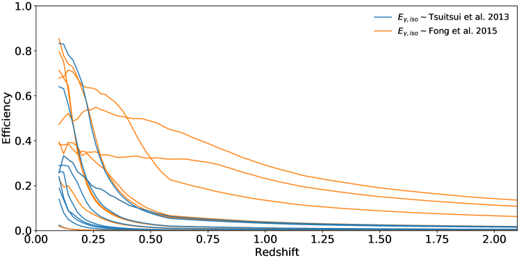
The efficiencies vary depending on a few factors. The total coverage and the limiting magnitude of the observations limit the maximum efficiency, which then decays depending on the associated $E_{iso}$. For larger energies, the decay is smoother. In the top panel of Fig. 9, we show the efficiencies for the 9 GRBs that had no discovered counterpart. We exclude GRB 200826A as the energies used to model the afterglow follow the SGRB energy distribution, while GRB 200826A was proven to be part of the LGRB population. The energies derived from the Tsutsui et al. (2013) relationship are larger than the mean $E_{K,iso}$ derived from Fong et al. (2015). This increases the efficiencies at larger redshifts assuming the Tsutsui et al. (2013) relationship, as the transients are intrinsically more energetic.

For both of the energies used, we calculate the joint probability of non-detection by taking the product of the SGRB ToO efficiencies as a function of redshift. Similar to the analysis in Kasliwal et al. (2020), we define

$$(1-CL)=\prod_{i=0}^{N}(1-p_{i})$$ (2)

with CL as the credible level and $p_{i}$ the efficiency of the i$th$ burst as a function of redshift. We show in the bottom panel of Fig. 9 the result for the afterglows with energies following Tsutsui et al. (2013) (blue) and Fong et al. (2015) (yellow). The lower energies associated with Fong et al. (2015) afterglows only allow us to probe the space up to z = 0.16, considering a $CL=0.9$, while SGRBs with energies following the $E_{iso}-E_{z,p}$ relationship can be probed as far as z = 0.4. To look into the prospects of the SGRB ToO campaign, we model a scenario with 21 additional ToO campaigns, each with a median efficiency based on the results presented here. These results are shown as dashed lines in Fig. 9, and show that for $E_{iso}\sim E_{K,iso}$, the improvement after thirty ToOs can only expand our searches (i.e. $CL=0.9$) up to z = 0.2, while if the GRBs follow the $E_{iso}-E_{z,p}$ relationship, our horizon expands to z = 0.7.

Finally, when comparing our limits to the redshift distribution of SGRB afterglows found in the literature (Fong et al., 2015) (green histogram in Fig. 9), our searches show that we are probing (and could probe) volumes that contain 10-40% of the observed afterglows, depending on the $E_{iso}$ assumption.

7 Proposed follow-up strategy

The current ToO strategy aims for two consecutive exposures in two different filters, prioritizing the color of the source as the main avenue to discriminate between sources. This helps confirming the nature of the transient as an extragalactic source. In some cases, it can lead to problems as the source might not be detected at shorter wavelengths, due to either the extinction along the line of sight or its intrinsically fainter brightness. If there is no second detection at shorter wavelengths, there is the risk of ignoring a potential counterpart as a single detection can be confused as a slow moving object or an artifact. The standard strategy considers a second night of ZTF observations in the same two filters, to measure the magnitude and color evolution. However, a number of sources did not have a second detection in the same filter after the second night, impeding the measurement of the decline rate. For these two reasons, for afterglow searches with ZTF (and possibly other instruments with similar limiting magnitudes), it is more informative to observe the region at least twice in the same filter during the first night. By separating the two same-filter epochs by at least $2\sigma\times 24/\alpha$, where $\sigma$ is the typical error of the observations and $\alpha$ is the power-law index of the afterglow decline, we can possibly measure the decay rate of sources, or at least set a lower limit for $\alpha$. For ZTF, two epochs separated by 6 hours would suffice for afterglows with a typical $\alpha\sim 1$, assuming $\sigma=0.12$.

This scenario is unlikely to happen often, as it requires that the region is visible during the entire night and that the night is long enough to allow for two visits separated by a number of hours. In any case, the standard ToO strategy for the second night of observation (two visits in two different filters) should help determine the color and magnitude evolution.

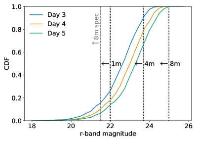
For the third day of follow-up, there will be two kinds of candidates: (a) confirmed fast fading transients, and (b) transients with unconstrained evolution, that likely only have data for the first night. For (a) it is important to get spectra as soon as possible before the transients fade below the spectroscopic limits. Ideally, observations in other wavelengths should be triggered to cement the classification and begin the characterization of the transient. For candidates in situation (b), the fast evolution of the transients requires the use of larger facilities. From our experience, this is feasible as only a handful of candidates will fall in this category. In both cases, (a) and (b), photometric follow-up using facilities different than ZTF are needed, as any afterglow detected by ZTF will likely not be detectable three days after the burst. In Fig. 10 we show the magnitude distribution of all the transients that simsurvey detected, independent of redshift, as a function of how many days passed after the burst. This figure illustrates the need for other telescopes to monitor the evolution of the transient, as for example, only $\sim$30% of the transients that we can detect with ZTF will be brighter than $r>22$ mag. Additionally, Fig. 10 shows that spectroscopy of the sources becomes harder after day 2, as only 20% of the detected transients will be brighter than $r=21.5$ mag.

Since spectroscopic data will be challenging to acquire for faint sources, the panchromatic follow-up, from radio to x-rays, will help to confirm the classification of the transient.

Figure 9: (top) The individual efficiency for each SGRB trigger. The blue curves are based on the $E_{iso}$ derived from the Band model $E_{p}$ and Eq. 1, while the yellow curves are the efficiencies assuming all GRBs have the same $E_{iso}$ as the mean $E_{K,iso}$ from Fong et al. (2015). (bottom) The solid lines represent the joint probability of non-detection using the 9 SGRB triggers with no optical counterparts. We adopt the same color coding as in the top plot, meaning blue for the $E_{iso}$ as a function of $E_{p}$ and yellow for $E_{iso}$ as the mean $E_{K,iso}$ from Fong et al. (2015). The dashed line represent the joint probability of non-detection after 30 ToOs, assuming an efficiency equal to the median efficiency of the ToOs presented. We show the cumulative redshift distribution for SGRBs as a green line. The grey dotted line shows the $CL=0.9$ level, at which the joint probability of non detection is $1-CL=0.1$.

Figure 10: The magnitude cumulative distribution of the sources detected using simsurvey as a function of the days after the burst. This distribution contains all the sources detected up to z$=2$. The photometric and spectroscopic limits of different facilities are shown as dotted vertical lines.

8 Conclusions

During a period of $\sim 2$ years, a systematic, extended and deep search for the optical counterparts to Fermi-GBM SGRBs has been performed employing the Zwicky Transient Facility. The ZTF observations of 10 events followed-up are listed in Table 3 and no optical counterpart has yet been associated to a compact binary coalescence. However, our ToO strategy led to the discovery of the optical counterpart to GRB 200826A, which was ultimately revealed as the shortest-duration LGRB found to date (Ahumada et al., 2021).

This experiment complements previous studies (Singer et al., 2013, 2015; Coughlin et al., 2019a), and demonstrates the feasibility of studying the large sky areas derived from Fermi GBM by exploiting the wide field of view of ZTF. The average coverage was $\sim 60\%$ of the localization regions, corresponding to $\sim 950$ deg². The average amount of alerts in the targeted regions of the sky was over 20000, and we were able to reduce this figure to no more than 20 candidates per trigger. Thanks to the high cadence of ZTF we were able to achieve a median reduction in alerts of 0.03%. The effectiveness of the filtering criteria is comparable with the median reduction reached in Singer et al. (2015), even when the areas covered are almost orders of magnitude larger. The iPTF search for the optical counterparts to the long gamma-ray burst GRB 130702A covered 71 deg² and yielded 43 candidates (Singer et al., 2013).

This campaign has utilized ZTF capabilities to rapidly follow-up SGRB trigger, which has allowed us to explore the magnitude space and set constraints on SGRBs events. The average depth for ZTF 300s exposures is $r\sim 20.8$ which has allowed us to look for SGRB afterglows and GW170817-like KNe. From Fig. 10, it can be seen that future follow-ups would benefit both from a more rapid response and longer exposures.

By using computational tools like afterglowpy and simsurvey, we have quantified the efficiency of our ToO triggers. The ZTF efficiency drops quickly as the transient is located at further distances, and the magnitude limits only allow for detections up to z = 0.4, for energies following the Tsutsui et al. (2013) relation and z = 0.16 for bursts with energies equal to the mean $E_{iso}$ found by Fong et al. (2015), for a $CL=0.9$. Furthermore, when repeating the experiment 21 times (to complete 30 ToOs) and assuming a median efficiency $p_{med}$ for each new event, the horizons of our searches increase to z = 0.2 and 0.72 respectively.

Additionally, our simulations show that ZTF is no longer effective at following-up afterglows after three days following the burst. The fast fading nature of these transients requires deeper observations, and spectroscopic and panchromatic observations are helpful to reveal the nature of the candidates. Ideally, at least two observations in the same filter should be taken during the first night of observation, as afterglows and KNe fade extremely rapidly and they might not be observable 48 hrs after the burst. With this strategy we can hope to find another counterpart.

Table 3: Summary of the ZTF ToO triggers. We list the area covered with ZTF, as well as the corresponding credible region (C.R.) of the GBM map. We shown our time delay between the burst and the start of ZTF observations. For each trigger, we list the exposure time for night 1 and night 2, along with the filter sequence in parenthesis. The last two columns show the median $r-$band 5$\sigma$ limit and the number of objects followed-up with other facilities.

GRB	Area covered	C.R. covered	Time delay in triggering ZTF	Exposure time (sequence)	$r-$band 5$\sigma$ limit	Objects followed-up
GRB 180523B	2900 $deg^{2}$	60%	9.1h	60s(rgr), 90s(rgr)	r $>$ 20.3 mag	14
GRB 180626C	275 $deg^{2}$	87%	1.5h	120s(rgr), 240s(grg)	r $>$ 20.9 mag	1
GRB 180715B	254 $deg^{2}$	37%	10.3h	180s(rgr), 240s(rg)	r $>$ 21.4 mag	14
GRB 180728B	334 $deg^{2}$	76%	31h	180s(rgr), 180s(rgr)	r $>$ 18.7 mag	7
GRB 180913A	546 $deg^{2}$	53%	8.3h	180s(grg), 300s(grg)	r $>$ 22.2 mag	12
GRB 181126B	1400 $deg^{2}$	66%	1.3h	180s(rr), 300s (r)	r $>$ 20.5 mag	11
GRB 200514B	519 $deg^{2}$	49%	0.9h	300s(gr)	r $>$ 22.2 mag	14
GRB 201130A	400 $deg^{2}$	75%	7h	300s(grg),300s(gr)	r $>$ 20.3 mag	0
GRB 210510A	1105 $deg^{2}$	84%	10h	180(gr),240(r)	r $>$ 22.1 mag	1

Table 4: Follow-up table of the candidates identified for GRB 180523B (Coughlin et al., 2018b), GRB 180626C (Coughlin et al., 2018a), GRB 180715B (Cenko et al., 2018), GRB 180913A (Coughlin et al., 2018b), GRB 181126B (Ahumada et al., 2018), GRB 200514B (Ahumada et al., 2020; Reusch et al., 2020a), and GRB 210510A (Anand et al., 2021). The spectroscopic (s) or photometric (p) redshifts of the respective host galaxies are listed as well. The photometric slow evolution of some candidates was used as a rejection criteria when the object presents a variation on its magnitude smaller than 0.3 mag/day.

GRB trigger	ZTF Name	RA	Dec	Discovery magnitude	Redshift	Rejection criteria
GRB 180523B	ZTF18aawozzj	12:31:09.02	+57:35:01.8	g = 20.20	(s) 0.095	SN Ia-91T P200
	ZTF18aawnbgg	10:40:54.05	+23:44:43.3	r = 19.80	(s) 0.135	SN Ia P200
	ZTF18aawmvbj	10:12:41.17	+21:24:55.5	r = 19.75	(s) 0.14	SN Ia P200
	ZTF18aawcwsx	10:40:33.46	+47:02:24.4	r = 19.84	(s) 0.09	SN Ia-91T P60
	ZTF18aawnbkw	10:38:47.66	+26:18:51.8	r = 19.91	(p) 0.31	slow SDSS
	ZTF18aawmqwo	09:52:06.90	+47:18:34.8	r = 19.98	(p) 0.04	slow SDSS
	ZTF18aawmkik	08:51:11.45	+13:13:16.7	r = 19.04	(p) 0.52	slow SDSS
	ZTF18aawnmlm	11:03:11.38	+42:07:29.9	r = 20.12	orphan	slow flat in 7 days
	ZTF18aauhzav	10:59:29.32	+44:10:02.7	r = 19.97	(s) 0.05	slow 2MASX
	ZTF18aavrhqs	11:58:09.57	+63:45:34.6	r = 19.99	orphan	slow
	ZTF18aawmwwk	10:35:26.51	+65:22:34.3	r = 19.99	(p) 0.18	slow SDSS
	ZTF18aawwbwm	08:16:44.98	+35:34:13.1	r = 19.79	(p) 0.15	slow SDSS
	ZTF18aawmjru	08:39:11.39	+44:01:53.6	r = 18.43	(p) 0.44	slow SDSS
	ZTF18aawmigr	08:48:01.76	+29:13:51.9	r = 19.63	(s) 0.1	slow 2MASX
GRB 180626C	ZTF18aauebur	19:48:49.10	+46:30:36.1	r = 18.85	stellar	CV multiple previous bursts
GRB 180715B	ZTF18aamwzlv	13:06:44.59	+68:59:52.9	r = 18.50	(s) 0.1	slow
	ZTF18abhbevp	14:21:00.83	+72:11:43.8	g = 20.63	–	slow
	ZTF18abhbpkm	16:02:36.78	+70:47:05.1	g = 21.24	–	slow
	ZTF18abhhjyd	13:02:32.07	+75:16:49.4	g = 20.43	–	AGN Milliquas match
	ZTF18abhbgan	15:43:18.86	+72:05:24.8	g = 21.22	orphan	slow
	ZTF18abhbfoi	13:24:34.01	+70:56:47.5	g = 21.12	(s )1.2	AGN Milliquas and PS1
	ZTF18abhbcjy	14:20:50.39	+73:25:40.5	g = 20.78	–	slow
	ZTF18abhaogg	13:42:45.47	+74:19:38.3	r = 20.38	orphan	slow
	ZTF18abhbamj	15:26:58.78	+72:02:17.8	r = 21.27	orphan	slow
	ZTF18abhawjn	13:31:27.33	+66:46:45.4	g = 20.69	(s) 0.4	AGN Milliquas
	ZTF18abharzk	13:41:09.05	+70:43:06.8	r = 21.30	–	slow
	ZTF18abhbckn	12:49:53.85	+73:02:00.5	r = 20.93	(s) 0.00541	slow CLU
	ZTF18abhbfqf	13:16:00.24	+69:37:24.1	r = 19.80	(s) 0.11	SN Ia-91T P200
	ZTF18aauhpyb	13:21:45.49	+70:55:59.8	g = 19.67	stellar	CV multiple bursts P60
GRB 180913A	ZTF18abvzgms	23:37:50.57	+47:53:21.2	g = 21.29	(p) 0.35	flat evolution SDSS
	ZTF18abwiios	23:12:14.06	+39:27:50.6	g = 22.04	–	flat evolution
	ZTF18abvzfgy	23:16:15.20	+43:31:59.3	g = 20.98	(s) 0.04	SN Ic LDT
	ZTF18abvzjwk	22:30:32.49	+39:50:14.6	g = 21.70	–	flat evolution
	ZTF18abvwhkl	23:05:44.17	+45:32:34.8	r = 21.44	–	flat evolution 3 points
	ZTF18abvucnv	22:31:31.96	+39:30:03.7	r = 21.15	stellar	Star flare
	ZTF18abwiitm	23:15:27.61	+39:57:10.5	g = 21.71	–	slow AGN WISE
	ZTF18abvubdm	22:58:28.45	+47:06:03.8	g = 21.01	–	slow evolution nice lc
	ZTF18abvzsld	00:15:57.12	+49:28:51.0	g = 21.50	Stellar	flat evolution
	ZTF18abwiivr	22:52:15.80	+37:22:29.4	g = 21.73	Stellar	slow evolution
	ZTF18abvzmtm	23:55:13.07	+48:21:37.8	g = 21.65	–	slow
GRB 181126B	ZTF18achtkfy	06:54:02.63	+37:04:28.6	g = 19.69	orphan	slow
	ZTF18achflqs	04:41:09.49	+23:53:24.9	r = 20.20	(p) 0.38	flat evolution SDSS
	ZTF18acrkcxa	04:55:02.52	+22:40:43.4	r = 20.85	Stellar	Flare Keck LRIS
	ZTF18acrkkpc	06:23:15.56	+10:19:22.6	r = 20.17	(s) 0.061	SN II Keck LRIS
	ZTF18aadwfrc	06:17:18.02	+50:29:03.3	r = 19.65	(s) 0.04	SN Ia-02cx Keck LRIS
	ZTF18acrfond	03:59:26.95	+24:35:20.4	r = 10.13	(s) 0.117	SN Ia Keck LRIS
	ZTF18acrfymv	06:18:01.18	+44:10:52.7	g = 20.82	(s) 0.072	SN Ic-BL Keck LRIS
	ZTF18acptgzz	04:33:32.45	-01:38:51.1	r = 19.56	(s) 0.096	SN Ia Keck LRIS
	ZTF18acbyrll	05:55:28.67	+29:28:20.3	r = 19.34	–	slow evolution
	ZTF18acrewzd	04:41:17.29	-01:46:07.5	g = 20.74	(s) 0.13	SN Ia Keck LRIS
GRB 200514B	ZTF20aazpphd	242.7149675	+27.1616870	r = 19.6	–	slow
	ZTF20aazppnv	238.1438691	+25.5764946	r = 21.1	(p) 0.17	slow
	ZTF20aazprjq	233.5213585	+43.3298714	r = 21.3	(p) 0.23	slow
	ZTF20aazptlp	229.007524	+48.774925	r = 21.5	(p) 0.40	slow
	ZTF20aazptnn	237.2967278	+47.271954	r = 21.6	(p) 0.26	slow
	ZTF20aazpnst	254.0989833	+34.4655542	r = 22.0	(p) 0.19	slow
	ZTF20aazpofi	236.929525	+46.9809542	r = 21.5	(p) 0.46	slow
	ZTF20aazplwp	2734.0167814	41.1672761	r = 21.6	–	slow
	ZTF20aazqlgx	2746.0908608	34.6259478	r = 22.3	(p) 0.35	slow
	ZTF20aazphye	2755.6577428	41.7013160	r = 21.6	(p) 0.26	slow
	ZTF20aazpnxd	2755.931646	48.3862806	r = 21.6	–	slow
	ZTF20aazpkri	2740.7324792	48.5554957	r = 21.3	–	slow
	ZTF20aazqndp	2737.8212032	50.4933039	r = 22.1	(s) 0.03	slow
	ZTF20aazqpps	2752.2388065	41.3097433	r = 21.6	(s) 0.2	slow
GRB 210510A	ZTF21abaytuk	13:48:49.89	+35:32:13.05	g = 21.76	(s) 0.8970	AGN Keck LRIS

References

- Abbott et al. (2017a) Abbott et al. 2017a, Phys. Rev. Lett., 119, 161101. https://link.aps.org/doi/10.1103/PhysRevLett.119.161101
- Abbott et al. (2017b) —. 2017b, The Astrophysical Journal Letters, 848, L13. http://stacks.iop.org/2041-8205/848/i=2/a=L13
- Abbott et al. (2017c) —. 2017c, Phys. Rev. Lett., 118, 221101
- Abbott et al. (2018) —. 2018, Living Reviews in Relativity, 21, 3. https://doi.org/10.1007/s41114-018-0012-9
- Ahumada et al. (2020a) Ahumada, R., Allende Prieto, C., Almeida, A., et al. 2020a, ApJS, 249, 3
- Ahumada et al. (2020b) Ahumada, T., Kumar, H., Fremling, C., et al. 2020b, GRB Coordinates Network, 29029, 1
- Ahumada et al. (2020c) —. 2020c, GRB Coordinates Network, 29029, 1
- Ahumada et al. (2018) Ahumada, T., Coughlin, M. W., Cenko, S. B., et al. 2018, GRB Coordinates Network, 23515, 1
- Ahumada et al. (2020) Ahumada, T., Anand, S., Andreoni, I., et al. 2020, GRB Coordinates Network, 27737, 1
- Ahumada et al. (2021) Ahumada, T., Singer, L. P., Anand, S., et al. 2021, Nature Astronomy, 5, 917
- Almualla et al. (2020) Almualla, M., Coughlin, M. W., Anand, S., et al. 2020, MNRAS, 495, 4366
- Amati (2021) Amati, L. 2021, Nature Astronomy, 5, 877
- Anand et al. (2021) Anand, S., Coughlin, M. W., Kasliwal, M. M., et al. 2021, Nature Astronomy, 5, 46
- Anand et al. (2021) Anand, S., Andreoni, I., Ahumada, T., et al. 2021, GRB Coordinates Network, 30005, 1
- Andreoni et al. (2019) Andreoni, I., Goldstein, D. A., Anand, S., et al. 2019, ApJ, 881, L16
- Andreoni et al. (2020) Andreoni, I., Goldstein, D. A., Kasliwal, M. M., et al. 2020, ApJ, 890, 131
- Andreoni et al. (2020) Andreoni, I., Kool, E. C., Carracedo, A. S., et al. 2020, The Astrophysical Journal, 904, 155
- Andreoni et al. (2021) Andreoni, I., Coughlin, M. W., Kool, E. C., et al. 2021, ApJ, 918, 63
- Arcavi et al. (2017) Arcavi, I., Hosseinzadeh, G., Howell, D. A., et al. 2017, Nature, 551, 64
- Ascenzi et al. (2019) Ascenzi, S., Coughlin, M. W., Dietrich, T., et al. 2019, MNRAS, 486, 672
- Band et al. (1993) Band, D., Matteson, J., Ford, L., et al. 1993, The Astrophysical Journal, 413, 281
- Bellm & Sesar (2016) Bellm, E. C., & Sesar, B. 2016, pyraf-dbsp: Reduction pipeline for the Palomar Double Beam Spectrograph, , , ascl:1602.002
- Bellm et al. (2019a) Bellm, E. C., Kulkarni, S. R., Graham, M. J., et al. 2019a, PASP, 131, 018002
- Bellm et al. (2019b) Bellm, E. C., Kulkarni, S. R., Barlow, T., et al. 2019b, PASP, 131, 068003
- Berger et al. (2005) Berger, E., Price, P. A., Cenko, S. B., et al. 2005, Nature, 438, 988
- Bertin & Arnouts (1996) Bertin, & Arnouts. 1996, Astron. Astrophys. Suppl. Ser., 117, 393. https://doi.org/10.1051/aas:1996164
- Blagorodnova et al. (2018) Blagorodnova, N., Neill, J. D., Walters, R., et al. 2018, PASP, 130, 035003
- Blondin & Tonry (2007) Blondin, S., & Tonry, J. L. 2007, ApJ, 666, 1024
- Bloom et al. (1999) Bloom, J. S., Kulkarni, S. R., Djorgovski, S. G., et al. 1999, Nature, 401, 453–456. http://dx.doi.org/10.1038/46744
- Bromberg et al. (2013) Bromberg, O., Nakar, E., Piran, T., & Sari, R. 2013, The Astrophysical Journal, 764, 179. http://stacks.iop.org/0004-637X/764/i=2/a=179
- Brown et al. (2013) Brown, T. M., Baliber, N., Bianco, F. B., et al. 2013, Publications of the Astronomical Society of the Pacific, 125, 1031. https://doi.org/10.1086%2F673168
- Bulla (2019) Bulla, M. 2019, MNRAS, 489, 5037
- Burns et al. (2021) Burns, E., Svinkin, D., Hurley, K., et al. 2021, The Astrophysical Journal Letters, 907, L28
- Cannizzo & Gehrels (2009) Cannizzo, J. K., & Gehrels, N. 2009, The Astrophysical Journal, 700, 1047. http://stacks.iop.org/0004-637X/700/i=2/a=1047
- Cano et al. (2017) Cano, Z., Wang, S.-Q., Dai, Z.-G., & Wu, X.-F. 2017, Advances in Astronomy, 2017
- Cenko et al. (2018) Cenko, S. B., Coughlin, M. W., Ghosh, S., et al. 2018, GRB Coordinates Network, 22969, 1
- Chambers et al. (2016) Chambers, K. C., Magnier, E. A., Metcalfe, N., et al. 2016, arXiv e-prints, arXiv:1612.05560
- Chatterjee et al. (2019) Chatterjee, D., Nugent, P. E., Brady, P. R., et al. 2019, The Astrophysical Journal, 881, 128
- Chornock et al. (2017) Chornock et al. 2017, The Astrophysical Journal Letters, 848, L19. http://stacks.iop.org/2041-8205/848/i=2/a=L19
- Côté et al. (2018) Côté, B., Fryer, C. L., Belczynski, K., et al. 2018, The Astrophysical Journal, 855, 99
- Coughlin et al. (2018a) Coughlin, M. W., Ahumada, T., Cenko, B., et al. 2018a, GRB Coordinates Network, 23379, 1
- Coughlin et al. (2018b) Coughlin, M. W., Singer, L. P., Cenko, S. B., et al. 2018b, GRB Coordinates Network, 22739, 1
- Coughlin et al. (2018) Coughlin, M. W., Tao, D., Chan, M. L., et al. 2018, Monthly Notices of the Royal Astronomical Society, 478, 692. http://dx.doi.org/10.1093/mnras/sty1066
- Coughlin et al. (2018a) Coughlin, M. W., Singer, L. P., Ahumada, T., et al. 2018a, GRB Coordinates Network, 22871, 1
- Coughlin et al. (2018b) Coughlin, M. W., Cenko, S. B., Ahumada, T., et al. 2018b, GRB Coordinates Network, 23324, 1
- Coughlin et al. (2019a) Coughlin, M. W., Ahumada, T., Cenko, S. B., et al. 2019a, PASP, 131, 048001
- Coughlin et al. (2019b) Coughlin, M. W., Ahumada, T., Anand, S., et al. 2019b, ApJ, 885, L19
- Coughlin et al. (2019a) Coughlin, M. W., Antier, S., Corre, D., et al. 2019a, Mon. Not. R. Astron. Soc., http://oup.prod.sis.lan/mnras/advance-article-pdf/doi/10.1093/mnras/stz2485/29808472/stz2485.pdf, stz2485. https://doi.org/10.1093/mnras/stz2485
- Coughlin et al. (2019b) Coughlin, M. W., Dekany, R. G., Duev, D. A., et al. 2019b, Monthly Notices of the Royal Astronomical Society, 485, 1412–1419. http://dx.doi.org/10.1093/mnras/stz497
- Coulter et al. (2017) Coulter, D. A., Foley, R. J., Kilpatrick, C. D., et al. 2017, Science, 358, 1556
- Cowperthwaite et al. (2017) Cowperthwaite, P. S., Berger, E., Villar, V. A., et al. 2017, ApJ, 848, L17
- Cutri et al. (2013) Cutri, R. M., Wright, E. L., Conrow, T., et al. 2013, Explanatory Supplement to the AllWISE Data Release Products, Explanatory Supplement to the AllWISE Data Release Products, ,
- D’Avanzo (2015) D’Avanzo, P. 2015, Journal of High Energy Astrophysics, 7, 73
- De et al. (2020) De, K., Hankins, M. J., Kasliwal, M. M., et al. 2020, PASP, 132, 025001
- Dekany et al. (2020) Dekany, R., Smith, R. M., Riddle, R., et al. 2020, PASP, 132, 038001
- Dichiara et al. (2020) Dichiara, S., Troja, E., O’Connor, B., et al. 2020, Monthly Notices of the Royal Astronomical Society, 492, 5011
- Dietrich et al. (2020) Dietrich, T., Coughlin, M. W., Pang, P. T. H., et al. 2020, Science, 370, 1450
- Drake et al. (2009) Drake, A., Djorgovski, S., Mahabal, A., et al. 2009, The Astrophysical Journal, 696, 870
- Drout et al. (2017) Drout, M. R., Piro, A. L., Shappee, B. J., et al. 2017, Science, 358, 1570
- Duev et al. (2019) Duev, D. A., Mahabal, A., Masci, F. J., et al. 2019, Monthly Notices of the Royal Astronomical Society, 489, 3582
- Duffell & MacFadyen (2015) Duffell, P. C., & MacFadyen, A. I. 2015, The Astrophysical Journal, 806, 205. http://stacks.iop.org/0004-637X/806/i=2/a=205
- Evans et al. (2017) Evans, P. A., Cenko, S. B., Kennea, J. A., et al. 2017, Science, 358, 1565
- Feindt et al. (2019) Feindt, U., Nordin, J., Rigault, M., et al. 2019, Journal of Cosmology and Astroparticle Physics, 2019, 005
- Flesch (2019) Flesch, E. W. 2019, arXiv e-prints, arXiv:1912.05614
- Fong et al. (2015) Fong, W., Berger, E., Margutti, R., & Zauderer, B. A. 2015, The Astrophysical Journal, 815, 102. http://stacks.iop.org/0004-637X/815/i=2/a=102
- Fong et al. (2016) Fong, W., Margutti, R., Chornock, R., et al. 2016, ApJ, 833, 151
- Fong et al. (2021) Fong, W., Laskar, T., Rastinejad, J., et al. 2021, ApJ, 906, 127
- Fremling et al. (2016) Fremling, C., Sollerman, J., Taddia, F., et al. 2016, A&A, 593, A68
- Gal-Yam et al. (2006) Gal-Yam, A., Fox, D., & MacFayden, A. 2006, Nature, 1053. https://doi.org/10.1038/nature05373
- Goldstein et al. (2017) Goldstein, A., Veres, P., Burns, E., et al. 2017, The Astrophysical Journal Letters, 848, L14
- Goldstein et al. (2020) Goldstein, A., Fletcher, C., Veres, P., et al. 2020, The Astrophysical Journal, 895, 40
- Goldstein et al. (2019) Goldstein, D. A., Andreoni, I., Nugent, P. E., et al. 2019, ApJ, 881, L7
- Gompertz et al. (2018) Gompertz, B., Levan, A., Tanvir, N., et al. 2018, The Astrophysical Journal, 860, 62
- Graham et al. (2019) Graham, M. J., Kulkarni, S., Bellm, E. C., et al. 2019, Publications of the Astronomical Society of the Pacific, 131, 078001
- Hamburg et al. (2018) Hamburg, R., Veres, P., & Meegan, C. 2018, GCN, 23057, 1
- Harris et al. (2020) Harris, C. R., Millman, K. J., van der Walt, S. J., et al. 2020, Nature, 585, 357–362
- Ho et al. (2022) Ho, A. Y. Q., Perley, D. A., Yao, Y., et al. 2022, arXiv e-prints, arXiv:2201.12366
- Hosseinzadeh et al. (2019) Hosseinzadeh, G., Cowperthwaite, P. S., Gomez, S., et al. 2019, ApJ, 880, L4
- Hunter (2007) Hunter, J. D. 2007, Computing in Science Engineering, 9, 90
- Kasen et al. (2017) Kasen, D., Metzger, B., Barnes, J., Quataert, E., & Ramirez-Ruiz, E. 2017, Nature, 551, 80 EP . http://dx.doi.org/10.1038/nature24453
- Kasliwal et al. (2019) Kasliwal, M., Cannella, C., Bagdasaryan, A., et al. 2019, Publications of the Astronomical Society of the Pacific, 131, 038003
- Kasliwal et al. (2017) Kasliwal, M. M., Nakar, E., Singer, L. P., et al. 2017, Science, 358, 1559. http://science.sciencemag.org/content/358/6370/1559
- Kasliwal et al. (2020) Kasliwal, M. M., Anand, S., Ahumada, T., et al. 2020, The Astrophysical Journal, 905, 145
- Kilpatrick et al. (2017) Kilpatrick et al. 2017, Science, 358, 1583. http://science.sciencemag.org/content/358/6370/1583
- Klebesadel et al. (1973) Klebesadel, R. W., Strong, I. B., & Olson, R. A. 1973, The Astrophysical Journal Letters, 182, L85
- Kluyver et al. (2016) Kluyver, T., Ragan-Kelley, B., Pérez, F., et al. 2016, in Positioning and Power in Academic Publishing: Players, Agents and Agendas, ed. F. Loizides & B. Scmidt (Netherlands: IOS Press), 87–90. https://eprints.soton.ac.uk/403913/
- Kotani et al. (2005) Kotani, T., Kawai, N., Yanagisawa, K., et al. 2005, Nuovo Cimento C Geophysics Space Physics C, 28, 755
- Kouveliotou et al. (1993) Kouveliotou, C., Meegan, C. A., Fishman, G. J., et al. 1993, The Astrophysical Journal, 413, L101
- Kumar & Granot (2003) Kumar, P., & Granot, J. 2003, The Astrophysical Journal, 591, 1075
- Labrie et al. (2019) Labrie, K., Anderson, K., Cárdenes, R., Simpson, C., & Turner, J. E. H. 2019, in Astronomical Society of the Pacific Conference Series, Vol. 523, Astronomical Data Analysis Software and Systems XXVII, ed. P. J. Teuben, M. W. Pound, B. A. Thomas, & E. M. Warner, 321
- Lattimer & Schramm (1974) Lattimer, J. M., & Schramm, D. N. 1974, ApJ, 192, L145
- Law et al. (2009) Law et al. 2009, Publications of the Astronomical Society of the Pacific, 121, 1395. http://stacks.iop.org/1538-3873/121/i=886/a=1395
- Lazzati et al. (2017) Lazzati, D., López-Cámara, D., Cantiello, M., et al. 2017, The Astrophysical Journal Letters, 848, L6. http://stacks.iop.org/2041-8205/848/i=1/a=L6
- Li & Paczynski (1998) Li, L.-X., & Paczynski, B. 1998, The Astrophysical Journal Letters, 507, L59. http://stacks.iop.org/1538-4357/507/i=1/a=L59
- Lipunov et al. (2005) Lipunov, V., Kornilov, V., Krylov, A., et al. 2005, Astrophysics, 48, 389
- Lipunov et al. (2017) Lipunov et al. 2017, The Astrophysical Journal Letters, 850, L1. http://stacks.iop.org/2041-8205/850/i=1/a=L1
- MacFarlane & Dunham (2004) MacFarlane, M. J., & Dunham, E. W. 2004, Optical design of the Discovery Channel Telescope, , , doi:10.1117/12.550633
- Mahabal et al. (2019) Mahabal, A., Rebbapragada, U., Walters, R., et al. 2019, Publications of the Astronomical Society of the Pacific, 131, 038002. https://doi.org/10.1088%2F1538-3873%2Faaf3fa
- Masci et al. (2019) Masci, F. J., Laher, R. R., Rusholme, B., et al. 2019, PASP, 131, 018003
- McCully et al. (2017) McCully, C., Hiramatsu, D., Howell, D. A., et al. 2017, ApJ, 848, L32
- Meegan et al. (2009) Meegan, C., Lichti, G., Bhat, P. N., et al. 2009, The Astrophysical Journal, 702, 791. https://doi.org/10.1088%2F0004-637x%2F702%2F1%2F791
- Mészáros & Rees (1998) Mészáros, P., & Rees, M. J. 1998, The Astrophysical Journal Letters, 502, L105. http://stacks.iop.org/1538-4357/502/i=2/a=L105
- Metzger et al. (2011) Metzger, B. D., Giannios, D., Thompson, T. A., Bucciantini, N., & Quataert, E. 2011, Monthly Notices of the Royal Astronomical Society, 413, 2031. http://dx.doi.org/10.1111/j.1365-2966.2011.18280.x
- Metzger et al. (2010) Metzger, B. D., Martínez-Pinedo, G., Darbha, S., et al. 2010, Monthly Notices of the Royal Astronomical Society, 406, 2650
- Metzger et al. (1997) Metzger, M., Djorgovski, S., Kulkarni, S., et al. 1997, Nature, 387, 878
- Mong et al. (2021) Mong, Y., Ackley, K., Galloway, D., et al. 2021, Monthly Notices of the Royal Astronomical Society, 507, 5463
- Mooley et al. (2017) Mooley, K. P., Nakar, E., Hotokezaka, K., et al. 2017, Nature, 554, 207 EP . http://dx.doi.org/10.1038/nature25452
- Morrissey et al. (2007) Morrissey, P., Conrow, T., Barlow, T. A., et al. 2007, ApJS, 173, 682
- Muthukrishna et al. (2019) Muthukrishna, D., Parkinson, D., & Tucker, B. E. 2019, ApJ, 885, 85
- Nagakura et al. (2014) Nagakura, H., Hotokezaka, K., Sekiguchi, Y., Shibata, M., & Ioka, K. 2014, The Astrophysical Journal Letters, 784, L28. http://stacks.iop.org/2041-8205/784/i=2/a=L28
- Nakar (2007) Nakar, E. 2007, Phys. Rept., 442, 166
- Narayan et al. (1992) Narayan, R., Paczynski, B., & Piran, T. 1992, ApJ, 395, L83
- Nicholl et al. (2017) Nicholl et al. 2017, The Astrophysical Journal Letters, 848, L18. http://stacks.iop.org/2041-8205/848/i=2/a=L18
- Nordin et al. (2019) Nordin, J., Brinnel, V., Van Santen, J., et al. 2019, Astronomy & Astrophysics, 631, A147
- O’Connor et al. (2021) O’Connor, B., Troja, E., Dichiara, S., et al. 2021, MNRAS, 502, 1279
- Oke et al. (1995) Oke, J., Cohen, J., Carr, M., et al. 1995, Publications of the Astronomical Society of the Pacific, 107, 375
- Patterson et al. (2019) Patterson, M. T., Bellm, E. C., Rusholme, B., et al. 2019, PASP, 131, 018001
- Pérez & Granger (2007) Pérez, F., & Granger, B. E. 2007, Computing in Science and Engineering, 9, 21. https://ipython.org
- Pian et al. (2017) Pian, E., D’Avanzo, P., Benetti, S., et al. 2017, Nature, 551, 67
- Rastinejad et al. (2021) Rastinejad, J. C., Fong, W., Kilpatrick, C. D., et al. 2021, ApJ, 916, 89
- Rau et al. (2009) Rau et al. 2009, Publications of the Astronomical Society of the Pacific, 121, 1334. http://stacks.iop.org/1538-3873/121/i=886/a=1334
- Reusch et al. (2020a) Reusch, S., Ahumada, T., Anand, S., et al. 2020a, GRB Coordinates Network, 27745, 1
- Reusch et al. (2020b) Reusch, S., Andreoni, I., Kumar, H., et al. 2020b, GRB Coordinates Network, 28981, 1
- Rhodes et al. (2021) Rhodes, L., Fender, R., Williams, D. R. A., & Mooley, K. 2021, MNRAS, 503, 2966
- Rigault et al. (2019) Rigault, M., Neill, J. D., Blagorodnova, N., et al. 2019, Astronomy & Astrophysics, 627, A115. http://dx.doi.org/10.1051/0004-6361/201935344
- Rossi et al. (2020) Rossi, A., Stratta, G., Maiorano, E., et al. 2020, MNRAS, 493, 3379
- Rossi et al. (2021) Rossi, A., Rothberg, B., Palazzi, E., et al. 2021, arXiv e-prints, arXiv:2105.03829
- Rosswog (2015) Rosswog, S. 2015, Int. J. Mod. Phys., D24, 1530012
- Ryan et al. (2020) Ryan, G., Van Eerten, H., Piro, L., & Troja, E. 2020, The Astrophysical Journal, 896, 166
- Shappee et al. (2017) Shappee, B. J., Simon, J. D., Drout, M. R., et al. 2017, Science, 358, 1574
- Singer et al. (2013) Singer et al. 2013, The Astrophysical Journal Letters, 776, L34. http://stacks.iop.org/2041-8205/776/i=2/a=L34
- Singer et al. (2015) —. 2015, The Astrophysical Journal, 806, 52
- Smartt et al. (2017) Smartt et al. 2017, Nature, 551, 75 EP . http://dx.doi.org/10.1038/nature24303
- Steele et al. (2004) Steele, I. A., Smith, R. J., Rees, P. C., & Baker, I. P. 2004, The Liverpool Telescope: performance and first results, , , doi:10.1117/12.551456. https://doi.org/10.1117/12.551456
- Stein et al. (2021) Stein, R., Reusch, S., & Necker, J. 2021, desy-multimessenger/nuztf: v2.4.1, vv2.4.1, Zenodo, doi:10.5281/zenodo.5758176. https://doi.org/10.5281/zenodo.5758176
- Stein et al. (2021) Stein, R., Velzen, S. v., Kowalski, M., et al. 2021, Nature Astronomy, 5, 510
- Stern et al. (2012) Stern, D., Assef, R. J., Benford, D. J., et al. 2012, The Astrophysical Journal, 753, 30. http://stacks.iop.org/0004-637X/753/i=1/a=30
- Svinkin et al. (2020) Svinkin, D., Golenetskii, S., Aptekar, R., et al. 2020, GRB Coordinates Network, 27755, 1
- Tachibana & Miller (2018) Tachibana & Miller. 2018, Submitted to PASP
- Tanvir et al. (2017) Tanvir, N. R., Levan, A. J., González-Fernández, C., et al. 2017, ApJ, 848, L27
- Tonry (2011) Tonry, J. L. 2011, Publ. Astron. Soc. Pac., 123, 58
- Troja et al. (2017) Troja, E., Piro, L., van Eerten, H., et al. 2017, Nature, 551, 71 EP . http://dx.doi.org/10.1038/nature24290
- Troja et al. (2019) Troja, E., Castro-Tirado, A. J., Becerra González, J., et al. 2019, Monthly Notices of the Royal Astronomical Society, 489, 2104
- Tsutsui et al. (2013) Tsutsui, R., Yonetoku, D., Nakamura, T., Takahashi, K., & Morihara, Y. 2013, Monthly Notices of the Royal Astronomical Society, 431, 1398
- Van Rossum & Drake (2009) Van Rossum, G., & Drake, F. L. 2009, Python 3 Reference Manual (Scotts Valley, CA: CreateSpace)
- Vieira et al. (2020) Vieira, N., Ruan, J. J., Haggard, D., et al. 2020, The Astrophysical Journal, 895, 96
- von Kienlin et al. (2020) von Kienlin, A., Meegan, C. A., Paciesas, W. S., et al. 2020, ApJ, 893, 46
- Wijers et al. (1997) Wijers, R. A. M. J., Rees, M. J., & Mészáros, P. 1997, Monthly Notices of the Royal Astronomical Society, 288, L51. http://dx.doi.org/10.1093/mnras/288.4.L51
- Willingale et al. (2007) Willingale, R., O’Brien, P. T., Osborne, J. P., et al. 2007, The Astrophysical Journal, 662, 1093
- Woosley & Bloom (2006) Woosley, S. E., & Bloom, J. S. 2006, ARA&A, 44, 507
- Wright et al. (2010) Wright, E. L., Eisenhardt, P. R. M., Mainzer, A. K., et al. 2010, The Astronomical Journal, 140, 1868. http://stacks.iop.org/1538-3881/140/i=6/a=1868
- Yao et al. (2019) Yao, Y., Miller, A. A., Kulkarni, S., et al. 2019, The Astrophysical Journal, 886, 152
- Zackay et al. (2016) Zackay, B., Ofek, E. O., & Gal-Yam, A. 2016, ApJ, 830, 27
- Zhang & Choi (2008) Zhang, & Choi. 2008, Astronomy and Astrophysics, 484, 293. https://doi.org/10.1051/0004-6361:20079210
- Zhang et al. (2021) Zhang, B. B., Liu, Z. K., Peng, Z. K., et al. 2021, Nature Astronomy, 5, 911
- Zhang et al. (2012) Zhang, Z., Chen, D., & Huang, Y. 2012, The Astrophysical Journal, 755, 55
- Zhu et al. (2021) Zhu, J.-P., Yang, Y.-P., Zhang, B., Gao, H., & Yu, Y.-W. 2021, arXiv preprint arXiv:2110.10468