Frequency perturbation theory of bound states in the continuum
in a periodic waveguide

Abstract

In a lossless periodic structure, a bound state in the continuum (BIC) is characterized by a real frequency and a real Bloch wavevector for which there exist waves propagating to or from infinity in the surrounding media. For applications, it is important to analyze the high-$Q$ resonances that either exist naturally for wavevectors near that of the BIC or appear when the structure is perturbed. Existing theories provide quantitative results for the complex frequency (and the $Q$-factor) of resonant modes that appear/exist due to structural perturbations or wavevector variations. When a periodic structure is regarded as a periodic waveguide, eigenmodes are often analyzed for a given real frequency. In this paper, we consider periodic waveguides with a BIC, and study the eigenmodes for a given real frequency near the frequency of the BIC. It turns out that such eigenmodes near the BIC always have a complex Bloch wavenumber, but they may or may not be leaky modes that radiate out power laterally to infinity. These eigenmodes can also be the so-called complex modes that decay exponentially in the lateral direction. Our study is relevant for applications of BICs in periodic optical waveguides, and it is also helpful for analyzing photonic devices operating near the frequency of a BIC.

I Introduction

In recent years, bound states in the continuum (BICs) have been the central topic of many studies in photonics [1, 2, 3, 4]. For a structure with at least one open spatial direction, a photonic BIC is an eigenmode of the governing Maxwell’s equations satisfying two conditions: (1) it decays rapidly in the open spatial direction, and (2) at the same frequency as the BIC, there exist waves that propagate to or from infinity in the open spatial direction. For a periodic structure sandwiched between two homogeneous media, such as a photonic crystal slab [5, 6, 7, 8, 9, 10, 11, 12, 13, 14] or a periodic array of cylinders [15, 16, 17, 18, 19, 20, 21, 22], a BIC is characterized by its frequency and Bloch wavevector, the direction perpendicular to the periodic layer is the open spatial direction, and propagating diffraction orders compatible with the BIC frequency and wavevector are the waves that propagate to or from infinity. For optical waveguides with an invariant direction [23, 24, 25, 26], a BIC is characterized by its frequency and propagation constant.

Most applications of BICs are related to high-$Q$ resonances that exist near a BIC or appear when a BIC is destroyed. In a periodic structure, a resonant mode is an outgoing solution of the Maxwell’s equations with a real Bloch wavevector and a complex frequency [27, 28]. A high-$Q$ resonance leads to local field enhancement [29, 30, 31, 32, 33] and sharp features in scattering spectra [34, 35, 36, 37, 38, 39] that are useful for lasing, sensing, switching, nonlinear optics, etc. To obtain a high-$Q$ resonance, the standard way is to perturb the structure [40, 41, 42]. Actually, a structural perturbation does not always destroy a BIC. If the BIC is protected by a symmetry, it continues to exist when the structure is perturbed preserving the symmetry. Some BICs are not protected by symmetry in the sense of symmetry mismatch, but can nevertheless persist under certain structural perturbations [43, 44, 45, 46, 47]. In general, if a structural perturbation contains a sufficient number of parameters, a generic BIC can survive the perturbation if the parameters are properly tuned [48, 49]. On the other hand, high-$Q$ resonant modes naturally exist near a BIC in a periodic structure without any structural perturbation. In fact, a BIC is a special point in a band of resonant modes that depend on the Bloch wavevector continuously. For a lossless structure, the $Q$ factor of the resonant mode tends to infinity as its wavevector tends to that of the BIC. The asymptotic relation between the $Q$ factor and wavevector difference can be determined using a perturbation method [50, 51, 42]. It is known that for some special BICs, the $Q$ factor of the nearby resonant mode tends to infinity extremely quickly [42, 51, 52].

A periodic structure sandwiched between two homogeneous media can be considered as a periodic waveguide. Eigenmodes in optical waveguides are often analyzed for a given real frequency. In this paper, we study eigenmodes of a periodic waveguide for frequencies near the frequency of a BIC. For simplicity, we consider two-dimensional (2D) structures with a single periodic direction, and study only eigenmodes in the $E$ polarization. At a real frequency, a waveguide mode is either a guided mode that decays exponentially in the lateral direction or a leaky mode that radiates out power to infinity (also in the lateral direction). In the case of a periodic waveguide (with a periodicity along the waveguide axis), the propagation constant is the Bloch wavenumber in the periodic direction. For a lossless waveguide, regular guided modes below the light line have a real propagation constant and form bands that depend on the frequency continuously. A BIC is also a guided mode, but it lies above the light line and is usually an isolate point in the real wavenumber-frequency plane. For open lossless periodic waveguides, there exist guided modes with a complex propagation constant and they are the so-called complex modes [53]. A complex mode, like a complex eigenvalue of a real nonsymmetric matrix, exists because the periodic-waveguide eigenvalue problem for a given frequency is not self-adjoint. Complex modes are well-known for waveguides with shielded boundaries [54], but they also exist in open lossless dielectric waveguides [55, 56, 57]. It should be emphasized that the complex propagation constant of a complex mode is not caused by material or radiation loss, and a complex mode is still a guided mode, since it decays exponentially in the lateral direction. A different kind of waveguide modes with a complex propagation constants are the well-known leaky modes [58, 59, 60]. Due to the radiation loss (power is radiated out in the lateral direction), the propagation constant of a leaky mode is always complex. Unlike a complex mode, the amplitude of a leaky mode grows exponentially in the lateral direction. Both complex and leaky modes form bands, and each band is given by the propagation constant being a complex-valued function of the real frequency. The purpose of this work is to reveal the connection between BICs and leaky or complex modes. Using a perturbation method, we show that when the frequency is perturbed, a BIC does not always become a leaky mode. In fact, it can also become a complex mode.

The rest of this paper is organized as follows. In Sec. II, we present a summary and an example for various eigenmodes in a periodic structure. In Sec. III, we use a perturbation method to analyze the waveguide modes near a BIC. Numerical examples are presented in Sec. IV to validate the perturbation theory. The paper is concluded with some comments in Sec. V.

II Eigenmodes in 2D periodic structures

In this section, we recall the definitions of various eigenmodes in 2D periodic structures and illustrate their connections by a numerical example. Consider a periodic structure that is invariant in $x$, periodic in $y$ with period $d$, bounded in $z$ by $|z|<h/2$ for some $h>0$, and surrounded by air. The dielectric function $\varepsilon$ is a real function of ${\bm{r}}=(y,z)$ and satisfies $\varepsilon(y+d,z)=\varepsilon({\bm{r}})$ for all ${\bm{r}}$, $\varepsilon({\bm{r}})=1$ for $|z|>h/2$, and $\max\varepsilon({\bm{r}})>1$. Two examples are shown in Fig. 1.

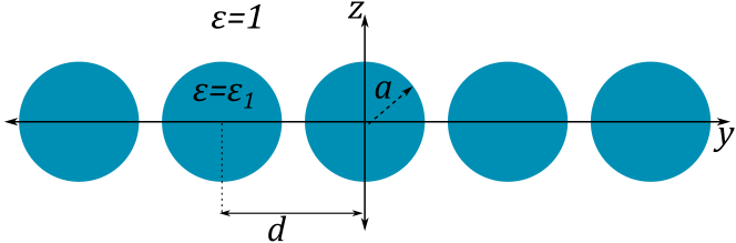
(a)

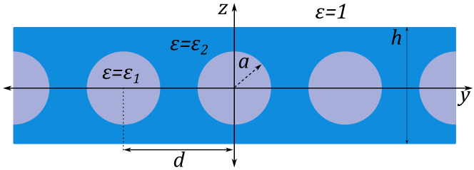
(b)

Figure 1: Schematic diagrams of two periodic structures with period $d$ along the $y$-axis.

Panel (a) shows a periodic array of circular cylinders with radius $a$ and dielectric constant $\varepsilon_{1}$, and panel (b) depicts a slab of thickness $h$ and dielectric constant $\varepsilon_{2}$, containing a periodic array of cylinders with radius $a$ and dielectric constant $\varepsilon_{1}$.

For the $E$-polarization, the $x$ component of the time-harmonic electric field, denoted as $u$, satisfies the following 2D Helmholtz equation:

$$\partial_{y}^{2}u+\partial_{z}^{2}u+k^{2}\varepsilon({\bm{r}})u=0,$$ (1)

where $k=\omega/c$ is the freespace wavenumber, $\omega$ is the angular frequency, and $c$ is the speed of light in vacuum, and the time dependence is $e^{-i\omega t}$. An eigenmode of such a periodic structure is a solution of Eq. (1) given by

$$u({\bm{r}})=\phi({\bm{r}})\,e^{i\beta y},$$ (2)

where $\beta$ is the Bloch wavenumber satisfying $\left|\mathrm{Re}(\beta)\right|\leq\pi/d$, and $\phi({\bm{r}})$ is periodic in $y$ with period $d$. In the free space given by $\left|z\right|>h/2$, the eigenmode can be expanded in plane waves as

$$u({\bm{r}})=\sum_{m=-\infty}^{\infty}\hat{u}_{m}^{\pm}e^{i(\beta_{m}y\pm\alpha_{m}z)},\quad\pm z>h/2,$$ (3)

where $\hat{u}_{m}^{\pm}$ are the expansion coefficients, $\beta_{0}=\beta$,

$$\beta_{m}=\beta+\frac{2\pi m}{d},\quad\alpha_{m}=\sqrt{k^{2}-\beta_{m}^{2}},$$ (4)

and the square root is defined using a branch cut along the negative imaginary axis.

An eigenmode must satisfy a proper boundary condition as $z\to\pm\infty$. If $\phi({\bm{r}})\to 0$ as $\left|z\right|\to\infty$, then the eigenmode is a guided mode. If both $\beta$ and $k$ are real, and $k<\left|\beta\right|$, the guided mode is a regular one below the light line. The regular guided modes form bands that depend on $\beta$ and $k$ continuously. A BIC is also a guided mode, but it is above the light line. More precisely, both $\beta$ and $k$ of a BIC are real and $k>|\beta|$. Since a BIC must decay as $z\to\pm\infty$, if for any $m$, $\alpha_{m}$ is real (note that at least $\alpha_{0}>0$), then $\hat{u}_{m}^{\pm}$ in Eq. (3) must vanish, because they are the coefficients of propagating plane waves. The periodic structure can also support complex modes which are guided modes with a complex $\beta$ [53]. Since the structure is non-absorbing and the field decays to zero as $z\to\pm\infty$, the complex modes are unrelated to absorption and radiation losses. They exist because the eigenvalue problem for a given frequency (where $\beta$ is the eigenvalue) is not self-adjoint [55]. The existence of complex modes is similar to the existence of complex eigenvalues for a real non-symmetric matrix.

Eigenmodes can also be defined using an outgoing radiation condition. In that case, the eigenmode radiates out power to infinity in the lateral direction, i.e., as $z\to\pm\infty$. A leaky mode is an eigenmode with a real $k$ and an outgoing wave field [58, 59, 60]. Since a leaky mode is losing power as it propagates forward, $\beta$ should have a positive imaginary part, so that the amplitude of the mode decays as it propagates forward. On the other hand, a complex $\beta$ implies that $\mbox{Im}(\alpha_{0})<0$, thus, the plane waves $\exp[i(\beta y\pm\alpha_{0}z)]$ blow up and the field of a leaky mode grows exponentially as $z\to\pm\infty$. A resonant mode is also an eigenmode satisfying the outgoing radiation condition, but it is given for a real $\beta$ [27, 28]. Since $\beta$ is real, the amplitude is uniform in the $y$ direction, to radiate out power to infinity in the lateral direction, a resonant mode must have a complex frequency (with a negative imaginary part), so that it decays with time. This implies that $\mbox{Im}(\alpha_{0})$ is also negative, and the field is unbounded as $z\to\pm\infty$.

To illustrate the different eigenmodes, we present an example for the periodic structure shown Fig. 1(b). For $\varepsilon_{1}=1$, $\varepsilon_{2}=11.56$, $h=1.8d$ and $a=0.25d$, we calculate the dispersion curves for various eigenmodes using a numerical method based on a nonlinear eigenvalue formulation [19, 20, 61]. The results are shown in Fig. 2.

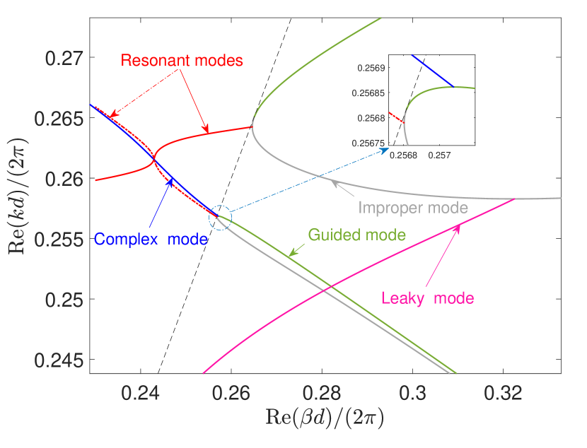
Figure 2: Normalized real parts of $k$ and $\beta$ for different modes near the light line. We show resonant (red), guided (green), improper (gray), leaky (purple) and complex (blue) mode curves.

The dispersion curves for regular guided, leaky, complex, resonant, and the so-called improper modes are shown as green, purple, blue, red, and gray curves, respectively. For resonant and complex/leaky modes, only the real parts of $k$ or $\beta$ are shown in the figure. The dashed line is the light line $k=\beta$. Two guided modes emerge from the light line tangentially. The dispersion curve of the lower guided mode has a local maximum where a complex mode appears [53]. An improper mode is a solution with a real $k$ and a real $\beta$, but it grows exponentially as $z\to\pm\infty$. Two improper modes emerge at the same points on the light line as the regular guided modes. A leaky mode appears at the minimum point on the dispersion curve of an improper mode [28]. The resonant modes are connected to the improper modes where the dispersion curves (of the improper modes) have an infinite slope [28]. At a particular value of $\beta$, the two resonant modes coalesce and form an exceptional point [61, 62].

III Perturbation analysis

In this section, we develop a perturbation theory for waveguide modes (leaky or complex modes) near a BIC in a periodic structure. As in Sec. II, we consider a 2D lossless periodic structure that is translationally invariant in $x$, periodic in $y$ with period $d$, and surrounded by air for $|z|>h/2$, and focus on $E$-polarized Bloch eigenmodes with a real frequency. Suppose the periodic structure supports a BIC $u_{*}({\bm{r}})=\phi_{*}({\bm{r}})e^{i\beta_{*}y}$ with Bloch wavenumber $\beta_{*}$ and frequency $\omega_{*}$ (freespace wavenumber $k_{*}=\omega_{*}/c$), we assume $k_{*}$ satisfies

$$|\beta_{*}|<k_{*}<\frac{2\pi}{d}-|\beta_{*}|,$$ (5)

then $\alpha_{*}=\sqrt{k_{*}^{2}-\beta_{*}^{2}}$ is positive, and for $m\neq 0$, $\alpha_{m}^{*}=[k_{*}^{2}-(\beta_{*}+2\pi m/d)^{2}]^{1/2}$ is pure imaginary with a positive imaginary part. This means that for the pair $\{\beta_{*},k_{*}\}$, there is only one radiation channel for positive or negative $z$, respectively. Now, for a given real $k$ near $k_{*}$, we seek a Bloch eigenmode $u({\bm{r}})=\phi({\bm{r}})e^{i\beta y}$ that either decays exponentially or radiates out power as $z\to\pm\infty$. In terms of $\phi$, Eq. (1) takes the form

$$\partial_{y}^{2}\phi+\partial_{z}^{2}\phi+2i\beta\partial_{y}\phi+[k^{2}\varepsilon({\bm{r}})-\beta^{2}]\phi=0.$$ (6)

Since the periodic structure is embedded in a homogeneous medium, a BIC is an isolated point in the real $\beta$-$k$ plane (when $d$ is the true minimum period of the structure), if $k\neq k_{*}$, $\beta$ is always complex. To find the Bloch mode with a complex $\beta$, we use a perturbation method assuming $|(\omega-\omega_{*})/\omega_{*}|=|(k-k_{*})/k_{*}|$ is small. For simplicity, we let $\delta=k^{2}-k_{*}^{2}$ and expand $\beta$ and $\phi$ in power series of $\delta$. It turns out that we need to use power series of $\sqrt{|\delta|}$ when the BIC carries zero power.

III.1 BIC with nonzero power

For $\delta\neq 0$, we seek $\beta$ and $\phi$ from the following power series:

$$\beta = \beta_{*}+\beta_{1}\delta+\beta_{2}\delta^{2}+\cdots,$$ (7)

$$\phi = \phi_{*}+\phi_{1}\delta+\phi_{2}\delta^{2}+\cdots.$$ (8)

Inserting the above into Eq. (6) and comparing terms of equal powers of $\delta$, we obtain

$$\mathcal{O}(1): \quad\mathcal{L}\phi_{*}=0,$$ (9)

$$\mathcal{O}(\delta): \quad\mathcal{L}\phi_{1}=2\beta_{1}(\beta_{*}\phi_{*}-i\partial_{y}\phi_{*})-\varepsilon({\bm{r}})\phi_{*},$$ (10)

$$\mathcal{O}(\delta^{2}): \quad\mathcal{L}\phi_{2}=2\beta_{1}(\beta_{*}\phi_{1}-i\partial_{y}\phi_{1})-\varepsilon({\bm{r}})\phi_{1}$$

$$\hskip 28.45274pt+2\beta_{2}(\beta_{*}\phi_{*}-i\partial_{y}\phi_{*})+\beta_{1}^{2}\phi_{*},$$

where $\mathcal{L}\equiv\partial_{y}^{2}+\partial_{z}^{2}+2i\beta_{*}\partial_{y}+k_{*}^{2}\varepsilon-\beta_{*}^{2}$.

Equation (9) is simply the governing equation of the BIC. The inhomogeneous equations (10) and (III.1) are singular and have no solution unless the right hand sides are orthogonal to $\phi_{*}$. Let $\Omega$ be the domain given by $0<y<d$ and $-\infty<z<\infty$. Multiplying $\overline{\phi}_{*}$ to both sides of Eq. (10) and integrating on $\Omega$, we obtain

$$\beta_{1}=\frac{1}{\mathcal{P}}\int_{\Omega}\varepsilon\left|\phi_{*}\right|^{2}d{\bm{r}},$$ (12)

where

$$\mathcal{P}=-2i\int_{\Omega}\overline{u}_{*}\frac{\partial u_{*}}{\partial y}d{\bm{r}},$$ (13)

and it is assumed to be nonzero. In Appendix, we show that $\mathcal{P}$ is real and proportional to the power carried by the BIC in the $y$ direction. Since we assume the BIC carries a nonzero power, $\mathcal{P}\neq 0$. It is clear that $\beta_{1}$ is real. In addition, we note that

$$\beta_{1}=\left.\frac{d\beta}{dk^{2}}\right|_{k=k_{*}}=\frac{1}{2k_{*}}\left.\frac{d\beta}{dk}\right|_{k=k_{*}}.$$

Thus, the slope of the dispersion curve at the BIC point is related to $\beta_{1}$.

To reveal the nature of this eigenmode, it is necessary to find the first term with a nonzero imaginary part in the power series of $\beta$. It is possible to write down a formula for $\beta_{2}$, but it is given in terms $\phi_{1}$ which satisfies Eq. (10). In Appendix, we show that the imaginary part of $\beta_{2}$ can be expressed (without involving $\phi_{1}$) as

$$\mathrm{Im}(\beta_{2})=\frac{\left|F_{1}\right|^{2}+\left|F_{2}\right|^{2}}{4d\alpha_{*}\mathcal{P}}$$ (14)

where $F_{1}$ and $F_{2}$ are given by

$$F_{j}=\int_{\Omega}\overline{\psi}_{j}({\bm{r}})G({\bm{r}})\,d{\bm{r}},\quad j=1,2,$$ (15)

$G({\bm{r}})=-2i\beta_{1}\partial_{y}\phi_{*}+[2\beta_{*}\beta_{1}-\varepsilon({\bm{r}})]\phi_{*}$ is the right hand side of Eq. (10), $\psi_{1}$ and $\psi_{2}$ are related to $w_{1}$ and $w_{2}$ by

$$w_{j}({\bm{r}})=\psi_{j}({\bm{r}})e^{i\beta_{*}y},\quad j=1,2,$$ (16)

$w_{1}$ and $w_{2}$ are diffraction solutions of Eq. (1) (with $k$ replaced by $k_{*}$) corresponding to incident waves $\exp[i(\beta_{*}y\pm\alpha_{*}z)]$ given for $z<-h/2$ and $z>h/2$, respectively.

We assume the BIC is generic in the sense that $(F_{1},F_{2})\neq(0,0)$. Since $\beta_{1}$ is real and $\mathrm{Im}(\beta_{2})\neq 0$, we have

$$\mathrm{Im}(\beta)=\mathcal{O}(\delta^{2})=\mathcal{O}(|\omega-\omega_{*}|^{2}).$$ (17)

If $\mathcal{P}$ is positive, then $\beta_{1}$ is positive, the imaginary part of $\beta$ is positive, $\alpha_{0}=\sqrt{k^{2}-\beta^{2}}$ has a negative imaginary part, the plane wave $e^{i(\beta y+\alpha_{0}z)}$ grows exponentially as $z\to+\infty$, and the eigenmode is a leaky mode. On the other hand, if $\mathcal{P}<0$, then $\beta_{1}<0$, $\mathrm{Im}(\beta)<0$, $\mathrm{Im}(\alpha_{0})>0$, the plane wave $e^{i(\beta y+\alpha_{0}z)}$ decays exponentially as $z\to+\infty$, and the eigenmode is a complex mode. Therefore, if a BIC has a nonzero power, it is a special point on the dispersion curve for a band of eigenmodes with a complex $\beta$. If the power of the BIC is positive, then the dispersion curve has a positive slope at the BIC point and the eigenmodes are leaky modes. If the power of the BIC is negative, then the dispersion curve has a negative slope at the BIC point and the eigenmodes are complex modes. If we assume $\beta_{*}>0$, the BIC with a negative power is a backward wave.

III.2 BIC with zero power

If the BIC carries no power in the $y$ direction, the perturbation method based on power series of $\delta$ fails. For a typical standing wave with $\beta_{*}=0$, the power is indeed zero. Therefore, it is important to analyze this special case. To find the eigenmodes near a BIC with a zero power, we try power series in $\sqrt{|\delta|}$. It is convenient to introduce an integer $s$, such that $s=1$ if $\delta>0$ and $s=-1$ if $\delta<0$, and expand $\beta$ and $\phi$ as

$$\beta=\beta_{*}+\beta_{1}\sqrt{s\delta}+\beta_{2}\delta+\cdots,$$ (18)

$$\phi=\phi_{*}+\phi_{1}\sqrt{s\delta}+\phi_{2}\delta+\cdots.$$ (19)

Inserting the above expansions into Eq. (6) and collecting terms at the same order, we obtain the following equations for $\phi_{*}$, $\phi_{1}$ and $\phi_{2}$:

$$\mathcal{O}(1): \ \mathcal{L}\phi_{*}=0,$$ (20)

$$\mathcal{O}(\sqrt{|\delta|}): \ \mathcal{L}\phi_{1}=2\beta_{1}(\beta_{*}\phi_{*}-i\partial_{y}\phi_{*}),$$ (21)

$$\mathcal{O}(\delta): \ \mathcal{L}\phi_{2}=2s\beta_{1}(\beta_{*}\phi_{1}-i\partial_{y}\phi_{1})+s\beta_{1}^{2}\phi_{*}$$

$$+2\beta_{2}(\beta_{*}\phi_{*}-i\partial_{y}\phi_{*})-\varepsilon({\bm{r}})\phi_{*}.$$ (22)

Since the power of the BIC is zero, the right hand side of Eq. (21) is orthogonal to $\phi_{*}$, thus $\beta_{1}$ cannot be determined from the solvability condition of $\phi_{1}$. To remove the unknown $\beta_{1}$, we define $\hat{\phi}_{1}$ such that $\phi_{1}=\beta_{1}\hat{\phi}_{1}$, then $\hat{\phi}_{1}$ satisfies

$$\mathcal{L}\hat{\phi}_{1}=G({\bm{r}})=2\beta_{*}\phi_{*}-2i\partial_{y}\phi_{*}$$ (23)

Multiplying $\overline{\phi}_{*}$ to both sides of Eq. (22), replacing $\phi_{1}$ by $\beta_{1}\hat{\phi}_{1}$, and integrating on $\Omega$, we get

$$s\beta_{1}^{2}\int_{\Omega}\left[|\phi_{*}|^{2}+R({\bm{r}})\right]d{\bm{r}}=\int_{\Omega}\varepsilon({\bm{r}})|\phi_{*}|^{2}d{\bm{r}},$$ (24)

where $R({\bf r})=2\overline{\phi}_{*}(\beta_{*}\hat{\phi}_{1}-i\partial_{y}\hat{\phi}_{1})$. Multiplying Eq. (24) by $\overline{\beta}_{1}^{2}$, and comparing the imaginary parts of both sides, we obtain

$$\mathrm{Im}\left(\overline{\beta}_{1}^{2}\right)=s\left|\beta_{1}\right|^{4}\frac{\mathrm{Im}\int_{\Omega}R({\bm{r}})d{\bm{r}}}{\int_{\Omega}\varepsilon\left|\phi_{*}\right|^{2}d{\bm{r}}}.$$ (25)

In Appendix, we show that

$$\mathrm{Im}\int_{\Omega}R({\bm{r}})d{\bm{r}}=-\frac{|F_{1}|^{2}+|F_{2}|^{2}}{4d\alpha_{*}},$$ (26)

where $F_{1}$ and $F_{2}$ are defined as in Eq. (15) with a new $G({\bm{r}})$ given in Eq. (23). This leads to

$$\mathrm{Im}\left(\beta_{1}^{2}\right)=\frac{s\left|\beta_{1}\right|^{4}\left(|F_{1}|^{2}+|F_{2}|^{2}\right)}{4d\alpha_{*}\int_{\Omega}\varepsilon\left|\phi_{*}\right|^{2}d{\bm{r}}}.$$ (27)

Therefore, if the BIC satisfies the condition $(F_{1},F_{2})\neq(0,0)$, then $\beta_{1}$ has a nonzero imaginary part and

$$\mathrm{Im}(\beta)=\mathcal{O}(\sqrt{|\delta|})=\mathcal{O}(|\omega-\omega_{*}|^{1/2}).$$ (28)

For $k>k_{*}$, i.e., $s=1$, $\mathrm{Im}\left(\beta_{1}^{2}\right)$ is positive, thus $\beta_{1}$ is in the first or third quadrant of the complex plane. It is clear that Eq. (24) has two solutions for $\beta_{1}$. Let these two solutions be $\beta_{1}^{(1)}$ and $\beta_{1}^{(2)}$, where $\beta_{1}^{(1)}$ is in the first quadrant and $\beta_{1}^{(2)}=-\beta_{1}^{(1)}$ is in the third quadrant. If $\beta_{*}$ of the BIC is positive, then the mode corresponding to $\beta_{1}^{(1)}$ has a positive $\mbox{Re}(\beta)$, a positive $\mbox{Im}(\beta)$, and a negative $\mbox{Im}(\alpha_{0})$, and it is a leaky mode; the mode corresponding to $\beta_{1}^{(2)}$ has a positive $\mbox{Re}(\beta)$, a negative $\mbox{Im}(\beta)$, a positive $\mbox{Im}(\alpha_{0})$, and it is a complex mode. The results are opposite if $\beta_{*}<0$. Since BICs with zero power are usually standing waves, the most important case is $\beta_{*}=0$. In that case, the two modes corresponding to $\beta_{1}^{(1)}$ and $\beta_{1}^{(2)}$ are both leaky modes, and they are reciprocal to each other.

If $k<k_{*}$, i.e., $s=-1$, then $\mathrm{Im}(\beta_{1}^{2})<0$, $\beta_{1}$ is in the second or fourth quadrant of the complex plane. Let the two solutions of Eq. (24) be $\beta_{1}^{(1)}$ (in the second quadrant) and $\beta_{1}^{(2)}=-\beta_{1}^{(1)}$ (in the fourth quadrant). For a BIC with $\beta_{*}>0$, the mode corresponding to $\beta_{1}^{(1)}$ has a positive $\mathrm{Re}(\beta)$, a positive $\mathrm{Im}(\beta)$, a negative $\mathrm{Im}(\alpha_{0})$, and it is a leaky mode; the mode corresponding to $\beta_{1}^{(2)}$ has a positive $\mathrm{Re}(\beta)$, a negative $\mathrm{Im}(\beta)$, a positive $\mathrm{Im}(\alpha_{0})$, and it is a complex mode. The opposite results are obtained for $\beta_{*}<0$. For $\beta_{*}=0$, the two modes corresponding to $\beta_{1}^{(1)}$ and $\beta_{1}^{(2)}$ are both complex modes.

IV Numerical results

In this section, we numerically verify the theoretical results obtained in the previous section. The first example is a periodic array of circular cylinders shown in Fig. 1(a). The dielectric constant and the radius of the cylinders are $\varepsilon_{1}=11.56$ and radius $a=0.3d$, respectively. For the $E$ polarization, the structure supports a few BICs. We consider three BICs that are shown as the small red dots and marked by ${\small\raisebox{-.9pt}1⃝}$, ${\small\raisebox{-.9pt}2⃝}$ and ${\small\raisebox{-.9pt}3⃝}$ in Fig. 3(a).

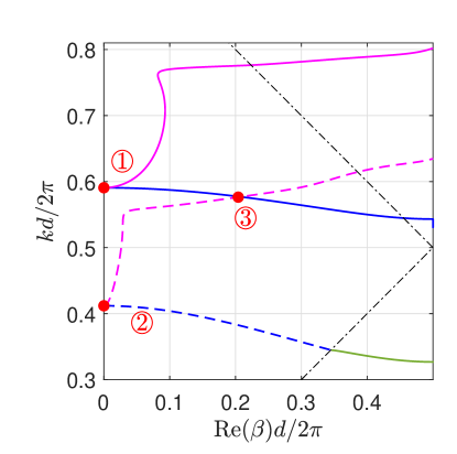
(a)

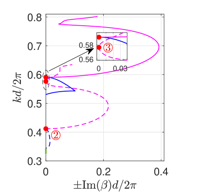
(b)

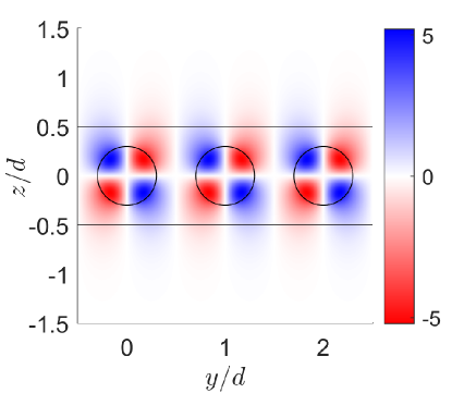
(c)

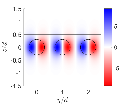
(d)

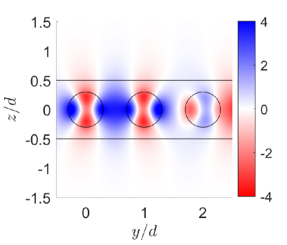
(e)

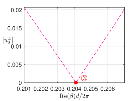
(f)

Figure 3: Example 1: a periodic array of circular cylinders. (a,b) Dispersion curves of complex (blue) and leaky (purple) modes, with BICs shown as the red dots: (a) $k$ versus $\mathrm{Re}(\beta)$, (b) $k$ versus $\mathrm{Im}(\beta)$. (c-e) Field profiles of BICs: (c) BIC $\raisebox{-.9pt}1⃝$, (d) BIC $\raisebox{-.9pt}2⃝$, (e) BIC $\raisebox{-.9pt}3⃝$. (f) Coefficient $\hat{u}_{0}^{\pm}$ of leaky modes near BIC $\raisebox{-0.9pt}3⃝$.

BICs ${\small\raisebox{-.9pt}1⃝}$ and ${\small\raisebox{-.9pt}2⃝}$ are anti-symmetric standing waves with $\beta_{*}=0$ and their electric fields are odd functions of $y$. The frequencies of BICs ${\small\raisebox{-.9pt}1⃝}$ and ${\small\raisebox{-.9pt}2⃝}$ are $\omega_{*}=0.5907(2\pi c/d)$ and $0.4119(2\pi c/d)$, respectively, and their field patterns [real part of $u_{*}(y,z)$] are shown in Figs. 3(c) and 3(d). BIC ${\small\raisebox{-.9pt}3⃝}$ is a propagating BIC with $\beta_{*}=0.2041(2\pi/d)$ and $\omega_{*}=0.5764(2\pi c/d)$. The field pattern of BIC ${\small\raisebox{-.9pt}3⃝}$ is quasi-periodic (not periodic) in $y$ and is shown in Fig. 3(e).

For BICs ${\small\raisebox{-.9pt}1⃝}$ and ${\small\raisebox{-.9pt}2⃝}$, we found leaky modes for $k>k_{*}$ and complex modes for $k<k_{*}$, in agreement with the perturbation theory of Sec. III(B). In Figs. 3(a) and 3(b), the dispersion curves of the leaky and complex modes are shown in purple and blue, respectively. For each band of leaky or complex modes, $\beta$ is a complex-valued function of $k$. The real and imaginary parts of $\beta$ are shown, as the horizontal axis, in Figs. 3(a) and 3(b), respectively. As $k$ is decreased from $k_{*}$, the complex mode emerged from BIC ${\small\raisebox{-.9pt}2⃝}$ ends below the light line [the black dashed line with positive slope in Fig. 3(a)] at a local maximum on the dispersion curve of a regular guided mode [53]. The solid green curve in Fig. 3(a) is the dispersion curve of the regular guided mode. The complex mode emerged from BIC ${\small\raisebox{-.9pt}1⃝}$ exists up to $\mathrm{Re}(\beta)=\pi/d$, and turns to a different complex mode with a fixed $\mathrm{Re}(\beta)=\pi/d$ [53]. The leaky modes emerged from these two BICs exist continuously as $k$ is increased and $\mathrm{Re}(\beta)$ passes $\pi/d$ with a finite derivative $d\beta/dk$.

On the dispersion curve of the leaky mode emerged from BIC ${\small\raisebox{-.9pt}2⃝}$, there is a special point with $\mathrm{Im}(\beta)=0$, and it is precisely BIC ${\small\raisebox{-.9pt}3⃝}$. Notice that this BIC is not on the dispersion curve of the complex mode emerged from BIC ${\small\raisebox{-.9pt}1⃝}$, since $\mathrm{Im}(\beta)$ of the complex mode at $k_{*}$ (of BIC ${\small\raisebox{-.9pt}3⃝}$) is clearly nonzero, as shown in Fig. 3(b). From Fig. 3(a), it is clear that $d\beta/dk>0$ at $k_{*}$. This is consistent with the theory developed in Sec. III(A). That is, $\beta_{1}$ is positive and the power of the BIC is positive. In Fig. 3(f), we show the radiation amplitude $\hat{u}_{0}^{\pm}$ [defined in Eq. (3)] of the leaky mode as a function of $\beta$. Since $\hat{u}_{0}^{\pm}$ depends on the scaling, we assume the leaky mode satisfies $u(y,h/2)=1$. It is clear that $\hat{u}_{0}^{\pm}=0$ for $\beta=\beta_{*}$. Therefore, as $k\to k_{*}$, $\mathrm{Im}(\beta)\to 0$, the leaky mode ceases to decay along the $y$-axis and it stops radiating power in the transverse direction.

The second example is a slab with a periodic array of air holes, as shown Fig. 1(b). The parameters are $\varepsilon_{1}=1$, $\varepsilon_{2}=11.56$, $a=0.3d$ and $h=d$. Like the first example, this periodic structure supports a few BICs. In Fig. 4(a),

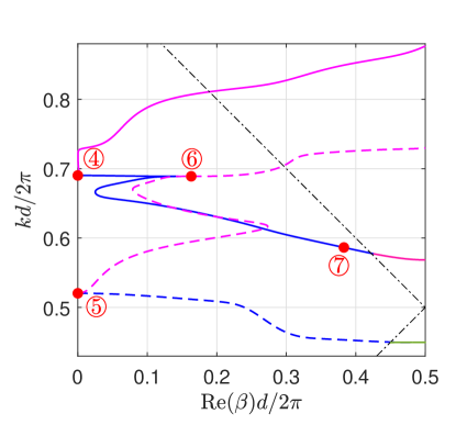
(a)

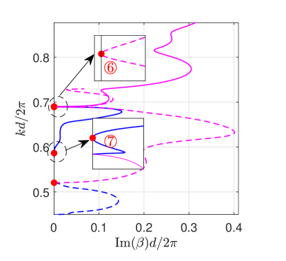
(b)

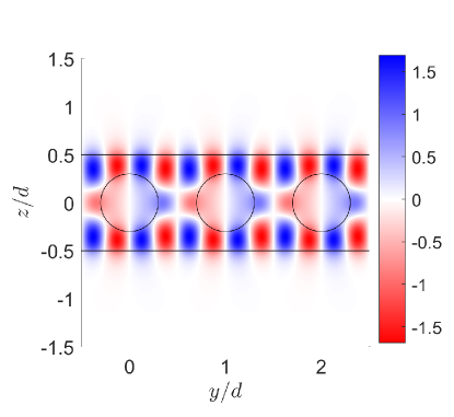
(c)

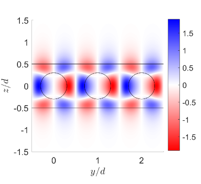
(d)

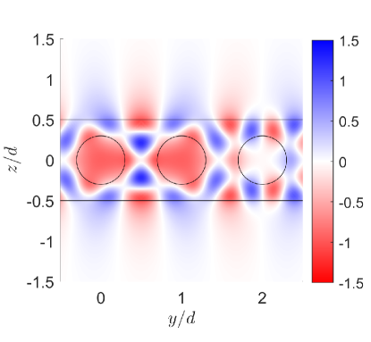
(e)

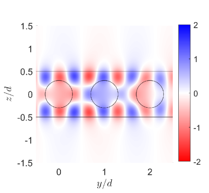
(f)

Figure 4: Example 2: a slab with a periodic array of air holes. (a,b) Dispersion curves of complex (blue) and leaky (purple) modes, with BICs shown as the red dots: (a) $k$ versus $\mathrm{Re}(\beta)$, (b) $k$ versus $\Im(\beta)$. (c-f): Field profiles of BICs: (c) BIC ${\small\raisebox{-.9pt}4⃝}$, (d) BIC ${\small\raisebox{-.9pt}5⃝}$, (e) BIC ${\small\raisebox{-.9pt}6⃝}$, (f) BIC ${\small\raisebox{-.9pt}7⃝}$.

four BICs are shown as the red dots and they are marked by ${\small\raisebox{-.9pt}4⃝}$, ${\small\raisebox{-.9pt}5⃝}$, ${\small\raisebox{-.9pt}6⃝}$ and ${\small\raisebox{-.9pt}7⃝}$, respectively. BICs ${\small\raisebox{-.9pt}4⃝}$ and ${\small\raisebox{-.9pt}5⃝}$ are anti-symmetric standing waves. Their frequencies are $\omega_{*}=0.6902(2\pi c/d)$ and $0.5204(2\pi c/d)$, respectively. The other two BICs are propagating BICs with a nonzero $\beta_{*}$. BIC ${\small\raisebox{-.9pt}6⃝}$ has Bloch wavenumber $\beta_{*}=0.1632(2\pi/d)$ and frequency $\omega_{*}=0.6890(2\pi c/d)$. For BIC ${\small\raisebox{-.9pt}7⃝}$, we have $\beta_{*}=0.3829(2\pi/d)$ and $\omega_{*}=0.5864(2\pi c/d)$.

As predicted by the theory developed in Sec. III(B), for each anti-symmetric standing wave, a leaky mode and a complex mode emerge at $\beta=0$ for $k>k_{*}$ and $k<k_{*}$, respectively. The complex mode emerged from BIC ${\small\raisebox{-.9pt}5⃝}$ ends at the maximum point on the dispersion curve of a regular guided mode below the light line [53]. The complex mode emerged from BIC ${\small\raisebox{-.9pt}4⃝}$ turns to a leaky mode at a transition point with a real $\beta$. This transition point corresponds to a special diffraction solution with incident wave from one diffraction channel and outgoing wave in a different radiation channel [53]. For the leaky and complex modes emerged from ${\small\raisebox{-.9pt}4⃝}$, the real and imaginary parts of $\beta$ have complicated dependence on $k$. The propagating BIC ${\small\raisebox{-.9pt}6⃝}$ lies on the dispersion curve of the leaky mode emerged from BIC ${\small\raisebox{-.9pt}5⃝}$. Consistent with the theory in Sec. III(A), this BIC has a positive power and the derivative $d\beta/dk$ is positive at $k_{*}$. The propagating BIC ${\small\raisebox{-.9pt}7⃝}$ appears on the dispersion curve of the complex mode emerged from BIC ${\small\raisebox{-.9pt}4⃝}$. Since $d\beta/dk$ is negative at $k_{*}$, BIC ${\small\raisebox{-.9pt}2⃝}$ has a negative power, consistent with the theory of Sec. III(A).

V Conclusion

In periodic structures, a BIC is often considered as a special state in a band of resonant modes with a real Bloch wavevector and a complex frequency, but for optical waveguides, eigenmodes are often studied for a given real frequency. In this paper, we showed that a BIC in a periodic waveguide is a special guided mode in a band of waveguide modes with a complex Bloch wavenumber $\beta$. While the complex-frequency modes near a BIC are all resonant modes radiating out power laterally, the waveguide modes with a complex $\beta$ can be leaky modes that radiate out power laterally or complex modes that decay exponentially in the lateral direction. These two cases are simply determined by the sign of the power carried by the BIC. If the BIC carries no power, as in the case of standing waves, both leaky and complex modes appear for frequencies near the frequency of the BIC.

Our study provides a useful guidance for applications of BICs in periodic optical waveguides. For simplicity, we studied only eigenmodes of $E$ polarization in 2D structures with a single periodic direction. Our theory can be extended to other wave-guiding structures with BICs, such as fibers with a periodic Bragg grating [63], periodic arrays of spheres or disks [64, 65], and uniform optical waveguides with lateral leaky channels [23, 26]. The current work is limited to generic cases so that $\mathrm{Im}(\beta)$ satisfies Eq. (17) or (28) for BICs with nonzero or zero power, respectively. It is probably useful to analyze non-generic BICs for which $\mathrm{Im}(\beta)$ exhibits higher order relations with the frequency difference.

Appendix

To find $\beta_{1}$ for subsection A of Sec. III, we multiply Eq. (9) by $\overline{\phi}_{*}$ and integrate on $\Omega$. Since $\phi_{*}$ satisfies $\mathcal{L}\phi_{*}=0$, standard integration by parts gives $\int_{\Omega}\overline{\phi}_{*}\mathcal{L}\phi_{1}d{\bm{r}}=0$. Therefore, $\mathcal{P}\beta_{1}=\int_{\Omega}\varepsilon|\phi_{*}|^{2}d{\bm{r}}$, where

$$\mathcal{P}=2\int_{\Omega}\overline{\phi}_{*}(\beta_{*}\phi_{*}-i\partial_{y}\phi_{*})d{\rm r}.$$

Since $\int_{\Omega}\partial_{y}(\overline{\phi}_{*}\phi_{*})d{\bm{r}}=0$, $\int_{\Omega}\overline{\phi}_{*}\partial_{y}\phi_{*}d{\bm{r}}$ is pure imaginary and thus $\mathcal{P}$ is real. Since $u_{*}=\phi_{*}e^{i\beta_{*}y}$, $\mathcal{P}$ is also given in Eq. (13). The power in the $y$ direction carried by the BIC is

$$P_{*}=\frac{1}{2Z_{0}k_{*}}\int_{-\infty}^{\infty}\mathrm{Im}(\overline{u}_{*}\partial_{y}u_{*})dz,$$ (A1)

where $Z_{0}$ is the free space impedance, and it is independent of $y$. Therefore, $\mathcal{P}=4dZ_{0}k_{*}P_{*}$.

Multiplying Eq. (III.1) by $\overline{\phi}_{*}$ and integrating on $\Omega$, we get

$$\mathcal{P}\beta_{2}+\beta_{1}^{2}\int_{\Omega}|\phi_{*}|^{2}d{\bm{r}}+\int_{\Omega}R({\bm{r}})d{\bm{r}}=0,$$ (A2)

where $R({\bm{r}})=\overline{\phi}_{*}[2\beta_{*}\beta_{1}\phi_{1}-2i\beta_{1}\partial_{y}\phi_{1}-\varepsilon({\bm{r}})\phi_{1}]$. It is easy to show that

$$\int_{\Omega}R({\bm{r}})d{\bm{r}}=\int_{\Omega}\phi_{1}\overline{G}({\bm{r}})d{\bm{r}}=\int_{\Omega}\phi_{1}\overline{\mathcal{L}\phi_{1}}d{\bm{r}},$$

where $G({\bm{r}})$ is the right hand side of Eq. (10). Therefore,

$$\mathcal{P}\,\mathrm{Im}(\beta_{2})=-\mathrm{Im}\int_{\Omega}\phi_{1}\overline{\mathcal{L}\phi_{1}}d{\bm{r}}.$$ (A3)

If $\phi_{1}$ has the far field expression

$$\phi(y,z)\sim b_{0}^{\pm}e^{i\alpha_{*}z},\quad z\to\pm\infty,$$

then we can show that

$$\mathrm{Im}\int_{\Omega}\phi_{1}\overline{\mathcal{L}\phi_{1}}d{\bm{r}}=-d\alpha_{*}(|b_{0}^{+}|^{2}+|b_{0}^{-}|^{2}).$$

Therefore,

$$\mathrm{Im}(\beta_{2})=\frac{d\alpha_{*}(|b_{0}^{+}|^{2}+|b_{0}^{-}|^{2})}{\mathcal{P}}.$$ (A4)

The functions $\psi_{1}$ and $\psi_{2}$ are related to diffraction solutions $w_{1}$ and $w_{2}$ by Eq. (16), and they have the following far field expressions

$$\psi_{1}({\bm{r}})\sim e^{i\alpha_{*}z}+R_{1}e^{-i\alpha_{*}z},\quad z\to-\infty,$$

$$\psi_{1}({\bm{r}})\sim T_{1}e^{i\alpha_{*}z},\quad z\to+\infty,$$

$$\psi_{2}({\bm{r}})\sim T_{2}e^{-i\alpha_{*}z},\quad z\to-\infty,$$

$$\psi_{2}({\bm{r}})\sim e^{-i\alpha_{*}z}+R_{2}e^{i\alpha_{*}z},\quad z\to+\infty,$$

where $R_{1}$, $R_{2}$, $T_{1}$ and $T_{2}$ are the reflection and transmission coefficients. Using these asymptotic expressions, we can calculate $F_{1}$ and $F_{2}$ satisfying

$$F_{j}=\int_{\Omega}\overline{\psi}_{j}G({\bm{r}})d{\bm{r}}=\int_{\Omega}\overline{\psi}_{j}\mathcal{L}\phi_{1}d{\bm{r}}.$$

The result can be written as

$$\begin{bmatrix}F_{1}\cr F_{2}\end{bmatrix}=2id\alpha_{*}\overline{S}\begin{bmatrix}b_{0}^{-}\cr b_{0}^{+}\end{bmatrix},\quad S=\begin{bmatrix}R_{1}&T_{2}\cr T_{1}&R_{2}\end{bmatrix}.$$ (A5)

The scattering matrix $S$ is unitary. Therefore,

$$|F_{1}|^{2}+|F_{2}|^{2}=4d^{2}\alpha_{*}^{2}(|b_{0}^{+}|^{2}+|b_{0}^{-}|^{2}).$$

Inserting the above into Eq. (A4), we get Eq. (14).

For subsection B of Sec. III, the functions $G$ and $R$ are defined differently. For $R({\bm{r}})$ given after Eq. (24), it is easy to show that

$$\int_{\Omega}R({\bm{r}})d{\bm{r}}=\int_{\Omega}\hat{\phi}_{1}\overline{G}({\bm{r}})d{\bm{r}}=\int_{\Omega}\hat{\phi}_{1}\overline{\mathcal{L}\hat{\phi}_{1}}d{\bm{r}}$$

where $G$ is given in Eq. (23). Following the same steps above, we get

$$\mathrm{Im}\int_{\Omega}\hat{\phi}_{1}\overline{\mathcal{L}\hat{\phi}_{1}}d{\bm{r}}=-\frac{|F_{1}|^{2}+|F_{2}|^{2}}{4d\alpha_{*}},$$ (A6)

where $F_{1}$ and $F_{2}$ are given by

$$F_{j}=\int_{\Omega}\overline{\psi}_{j}G({\bm{r}})d{\bm{r}}=\int_{\Omega}\overline{\psi}_{j}\mathcal{L}\hat{\phi}_{1}d{\bm{r}}.$$

The above leads to Eq. (26).

References

- [1] C. W. Hsu, B. Zhen, A. D. Stone, J. D. Joannopoulos, and M. Soljačić, “Bound states in the continuum,” Nat. Rev. Mater. 1, 16048 (2016).
- [2] K. Koshelev, G. Favraud, A. Bogdanov, Y. Kivshar, and A. Fratalocchi, “Nonradiating photonics with resonant dielectric nanostructures,” Nanophotonics 8, 725–745 (2019).
- [3] S. I. Azzam and A. V. Kildishev, “Photonic bound states in the continuum: from basics to applications,” Adv. Opt. Mater. 9, 2001469 (2021).
- [4] A. F. Sadreev, “Interference traps waves in an open system: bound states in the continuum,” Rep. Prog. Phys. 84, 055901 (2021).
- [5] P. Paddon and J. F. Young, “Two-dimensional vector-coupled-mode theory for textured planar waveguides,” Phys. Rev. B 61, 2090-2101 (2000).
- [6] T. Ochiai and K. Sakoda, “Dispersion relation and optical transmittance of a hexagonal photonic crystal slab,” Phys. Rev. B 63, 125107 (2001).
- [7] S. G. Tikhodeev, A. L. Yablonskii, E. A Muljarov, N. A. Gippius, and T. Ishihara, “Quasi-guided modes and optical properties of photonic crystal slabs,” Phys. Rev. B 66, 045102 (2002).
- [8] S. Shipman and D. Volkov, “Guided modes in periodic slabs: existence and nonexistence,” SIAM J. Appl. Math. 67, 687–713 (2007).
- [9] J. Lee, B. Zhen, S. L. Chua, W. Qiu, J. D. Joannopoulos, M. Soljačić, and O. Shapira, “Observation and differentiation of unique high-Q optical resonances near zero wave vector in macroscopic photonic crystal slabs,” Phys. Rev. Lett. 109, 067401 (2012).
- [10] C. W. Hsu, B. Zhen, J. Lee, S.-L. Chua, S. G. John- son, J. D. Joannopoulos, and M. Soljačić, “Observation of trapped light within the radiation continuum,” Nature 499, 188-191 (2013).
- [11] Y. Yang, C. Peng, Y. Liang, Z. Li, and S. Noda, “Analytical perspective for bound states in the continuum in photonic crystal slabs,” Phys. Rev. Lett. 113, 037401 (2014).
- [12] R. Gansch, S. Kalchmair, P. Genevet, T. Zederbauer, H. Detz, A. M. Andrews, W. Schrenk, F. Capasso, M. Lončar, and G. Strasser, “Measurement of bound states in the continuum by a detector embedded in a photonic crystal,” Light: Science & Applications 5, e16147 (2016).
- [13] W. Liu, B. Wang, Y. Zhang, J. Wang, M. Zhao, F. Guan, X. Liu, L. Shi, and J. Zi, “Circularly Polarized States Spawning from Bound States in the Continuum,” Phys. Rev. Lett. 123, 116104 (2019).
- [14] T. Yoda and M. Notomi, “Generation and Annihilation of Topologically Protected Bound States in the Continuum and Circularly Polarized States by Symmetry Breaking,” Phys. Rev. Lett. 125, 053902 (2020).
- [15] S. P. Shipman and S. Venakides, “Resonance and bound states in photonic crystal slabs,” SIAM J. Appl. Math. 64, 322-342 (2003).
- [16] R. Porter and D. Evans, “Embedded Rayleigh-Bloch surface waves along periodic rectangular arrays,” Wave Motion 43, 29-50 (2005).
- [17] D. C. Marinica, A. G. Borisov, and S. V. Shabanov, “Bound states in the continuum in photonics,” Phys. Rev. Lett. 100, 183902 (2008).
- [18] E. N. Bulgakov and A. F. Sadreev, “Bloch bound states in the radiation continuum in a periodic array of dielectric rods.” Phys. Rev. A 90, 053801 (2014).
- [19] Z. Hu and Y. Y. Lu, “Standing waves on two-dimensional periodic dielectric waveguides,” Journal of Optics 17, 065601 (2015).
- [20] L. Yuan and Y. Y. Lu, “Propagating Bloch modes above the lightline on a periodic array of cylinders,” J. Phys. B: Atomic, Mol. and Opt. Phys. 50, 05LT01 (2017).
- [21] Z. Hu, L. Yuan, and Y. Y. Lu, “Bound states with complex frequencies near the continuum on lossy periodic structures,” Phys. Rev. A 101, 013806 (2020).
- [22] A. Abdrabou and Y. Y. Lu, “Circularly polarized states and propagating bound states in the continuum in a periodic array of cylinders,” Phys. Rev. A 103, 043512 (2021).
- [23] C.-L. Zou, J.-M. Cui, F.-W. Sun, X. Xiong, X.-B. Zou, Z.- F. Han, and G.-C. Guo, “Guiding light through optical bound states in the continuum for ultrahigh- microresonantors,” Laser Photonics Rev. 9, 114-119 (2015).
- [24] J. Gomis-Bresco, D. Artigas, and L. Torner, “Anisotropy-induced photonic bound states in the continuum,” Nature Photonics, 11, 232-236 (2017).
- [25] S. Mukherjee, J. Gomis-Bresco, P. Pujol-Closa, D. Artigas, and L. Torner, “Topological properties of bound states in the continuum in geometries with broken anisotropy symmetry,” Phys. Rev. A 98, 063826 (2018).
- [26] L. Yuan and Y. Y. Lu, “On the robustness of bound states in the continuum in waveguides with lateral leakage channels,” Opt. Express 29, 16695-16709 (2021).
- [27] S. Fan and J. D. Joannopoulos, “Analysis of guided resonances in photonic crystal slabs,” Phys. Rev. B 65, 235112 (2002).
- [28] A. Abdrabou and Y. Y. Lu, “Indirect link between resonant and guided modes on uniform and periodic slabs,” Phys. Rev. A 99, 063818 (2019).
- [29] J. W. Yoon, S. H. Song, and R. Magnusson, “Critical field enhancement of asymptotic optical bound states in the continuum,” Sci. Rep. 5, 18301 (2015).
- [30] V. Mocella and S. Romano, “Giant field enhancement in photonic lattices,” Phys. Rev. B 92, 155117 (2015).
- [31] E. N. Bulgakov and D. N. Maksimov, “Light enhancement by quasi-bound states in the continuum in dielectric arrays,” Opt. Express 25, 14134-14147 (2017).
- [32] Z. Hu, L. Yuan, and Y. Y. Lu, “Resonant field enhancement near bound states in the continuum on periodic structures,” Phys. Rev. A 101, 043825 (2020).
- [33] L. Tan, L. Yuan, and Y. Y. Lu, “Resonant field enhancement in lossy periodic structures supporting complex bound states in the continuum,” J. Opt. Soc. Am. B 39 (2), 611–618 (2022).
- [34] S. P. Shipman and S. Venakides, “Resonant transmission near nonrobust periodic slab modes,” Phys. Rev. E 71, 026611 (2005).
- [35] N. A. Gippius, S. G. Tikhodeev, and T. Ishihara, “Optical properties of photonic crystal slabs with an asymmetrical unit cell,” Phys. Rev. B 72, 045138 (2005).
- [36] S. P. Shipman and H. Tu, “Total resonant transmission and reflection by periodic structures,” SIAM J. Appl. Math. 72(1), 216–239 (2012).
- [37] D. A. Bykov and L. L. Doskolovich, “- Fano line shape in photonics crystal slabs,” Phys. Rev. A 92, 013845 (2015).
- [38] C. Blanchard, J.-P. Hugonin, and C. Sauvan, “Fano resonant modes in photonic crystal slabs near optical bound states in the continuum,” Phys. Rev. B 94, 155303 (2016).
- [39] H. Wu, L. Yuan, and Y. Y. Lu, “Approximating transmission and reflection spectra near isolated nondegenerate resonances,” arXiv:2202.06324 (2022).
- [40] K. Koshelev, S. Lepeshov, M. Liu, A. Bogdanov, and Y. Kivshar, “Asymmetric metasurfaces with high- resonances governed by bound states in the contonuum,” Phys. Rev. Lett. 121, 193903 (2018)
- [41] Z. Hu and Y. Y. Lu, “Resonances and bound states in the continuum on periodic arrays of slightly noncircular cylinders,” J. Phys. B: At. Mol. Opt. Phys. 51, 035402 (2018).
- [42] L. Yuan and Y. Y. Lu, “Perturbation theories for symmetry-protected bound states in the continuum on two-dimensional periodic structures,” Phys. Rev. A 101, 043827 (2020).
- [43] B. Zhen, C. W. Hsu, L. Lu, A. D. Stone, and M. Soljačič, “Topological nature of optical bound states in the continuum,” Phys. Rev. Lett. 113, 257401 (2014).
- [44] E. N. Bulgakov and D. N. Maksimov, “Bound states in the continuum and polarization singularities in periodic arrays of dielectric rods,” Phys. Rev. A 96, 063833 (2017).
- [45] L. Yuan and Y. Y. Lu, “Bound states in the continuum on periodic structures: perturbation theory and robustness,” Opt. Lett. 42(21) 4490-4493 (2017).
- [46] L. Yuan and Y. Y. Lu, “Conditional robustness of propagating bound states in the continuum in structures with two-dimensional periodicity,” Phys. Rev. A 103 (4), 043507 (2021).
- [47] L. Yuan and Y. Y. Lu, “On the robustness of bound states in the continuum in waveguides with lateral leakage channels,” Opt. Express 29, 16695-16709 (2021).
- [48] L. Yuan and Y. Y. Lu, “Parametric dependence of bound states in the continuum on periodic structures,” Phys. Rev. A 102, 033513 (2020).
- [49] L. Yuan, X. Luo, and Y. Y. Lu, “Parametric dependence of bound states in the continuum in periodic structures: Vectorial cases,” Phys. Rev. A 104 (2), 023521 (2021).
- [50] L. Yuan and Y. Y. Lu, “Strong resonances on periodic arrays of cylinders and optical bistability with weak incident waves,” Phys. Rev. A 95, 023834 (2017).
- [51] L. Yuan and Y. Y. Lu, “Bound states in the continuum on periodic structures surrounded by strong resonances,” Phys. Rev. A 97(4), 043828 (2018).
- [52] J. Jin, X. Yin, L. Ni, M. Soljacic, B. Zhen, and C. Peng, “Topologically enabled unltrahigh- guided resonances robust to out-of-plane scattering,” Nature 574, 501-504 (2019).
- [53] A. Abdrabou and Y. Y. Lu, “Complex modes in an open lossless periodic waveguide,” Opt. Lett. 45(20), 5632–5635 (2020).
- [54] M. Mrozowski, Guided Electromagnetic Waves: Properties and Analysis (Research Studies Press Ltd., England, 1997)
- [55] T. F. Jabloński, “Complex modes in open lossless dielectric waveguides,” J. Opt. Soc. Am. A 11, 1272-1282 (1994).
- [56] H. Xie, W. Lu, and Y. Y. Lu, “Complex modes and instability of full-vectorial beam propagation methods,” Opt. Lett. 36, 2474–2476 (2011).
- [57] N. Zhang and Y. Y. Lu, “Complex modes in optical fibers and silicon waveguides,” Opt. Lett. 46(17), 4410–4413 (2021).
- [58] A. W. Snyder and J. D. Love, Optical Waveguide Theory (Chapman and Hall, London, UK, 1983).
- [59] C. Vassallo, Optical Waveguide Concepts (Elsevier, Amsterdam, 1991).
- [60] J. Hu and C. R. Menyuk, “Understanding leaky modes: slab waveguide revisited,” Advances in Optics and Photonics 1, 58-106 (2009).
- [61] A. Abdrabou and Y. Y. Lu, “Exceptional points of resonant states on a periodic slab,” Phys. Rev. A 97, 063822 (2018).
- [62] A. Abdrabou and Y. Y. Lu, “Exceptional points of Bloch eigenmodes on a dielectric slab with a periodic array of cylinders,” Physica Scripta 95(9), 095507 (2020).
- [63] X. Gao, B. Zhen, M. Soljacic, H. Chen, and C. W. Hsu, “Bound states in the continuum in fiber Bragg gratings,” ACS Photonics 6, 2996-3002 (2019).
- [64] E. N. Bulgakov and D. N. Maksimov, “Topological bound states in the continuum in arrays of dielectric spheres,” Phys. Rev. Lett. 118, 267401 (2017).
- [65] Z. F. Sadrieva, M. A. Belyakov, M. A. Balezin, P. V. Kapitanova, E. A. Nenasheva, A. F. Sadreev, and A. A. Bogdanov, “Experimental observation of a symmetry-protected bound state in the continuum in a chain of dielectric disks,” Phys. Rev. A 99, 053804 (2019).