Continuous Optimization for Control of Hybrid Systems with Hysteresis via Time-Freezing

Abstract

This article regards numerical optimal control of a class of hybrid systems with hysteresis using solely techniques from nonlinear optimization, without any integer variables. Hysteresis is a rate independent memory effect which often results in severe nonsmoothness in the dynamics. These systems are not simply Piecewise Smooth Systems (PSS); they are a more complicated form of hybrid systems. We introduce a time-freezing reformulation which transforms these systems into a PSS. From the theoretical side, this reformulation opens the door to study systems with hysteresis via the rich tools developed for Filippov systems. From the practical side, it enables the use of the recently developed Finite Elements with Switch Detection [1], which makes high accuracy numerical optimal control of hybrid systems with hysteresis possible. We provide a time optimal control problem example and compare our approach to mixed-integer formulations from the literature.

hybrid systems, optimal control, numerical algorithms

1 Introduction

Hysteresis occurs in many physical systems, e.g., ferromagnetism, plasticity, superconductivity, phase transitions, but also in feedback control, e.g., thermostats [2, 3]. Hysteresis effects in dynamic systems are modeled with nonsmooth differential equations. This paper focuses on transforming some classes of systems with hysteresis into piecewise smooth system (PSS) and numerically solving optimal control problems (OCP) with PSS. We leverage recent advances in numerical optimal control of PSS, namely we use the FESD method [1].

A hybrid system with hysteresis can be represented as a finite automaton [3] which has two modes of operation described by $f_{\mathrm{A}}(x)$ and $f_{\mathrm{B}}(x)$, cf. Fig. 1(a). If the system operates in mode ${\mathrm{A}}$ with $\dot{x}=f_{\mathrm{A}}(x)$ and if $\psi(x)\geq 1$, it switches to mode $\mathrm{B}$ with $\dot{x}=f_{{\mathrm{B}}}(x)$. On the other hand, if it operates in mode ${\mathrm{B}}$ and if $\psi(x)\leq 0$, it switches to mode ${\mathrm{A}}$. This is a typical hysteresis behavior given by the characteristic in Fig. 1(b), which is often called the delayed relay operator [4]. The dynamics of the system depend on the value of $w(t)$ and the scalar switching function $\psi(x)$. Notably, for $\psi(x)\in[0,1]$ the function $w(t)$ can be 0 or 1.

There are several other related characteristics, e.g. the dashed lines in Fig. 1(b) could be solid, or the resulting polygon in the middle of the plot might be tilted. In all these cases the characteristic can be readily represented via a linear complementarity problem [5] and the nonsmooth dynamic system recast into a Dynamic Complementarity System (DCS). However, it is an open question if this DCS is a PSS.

(a) Finite automaton of a hybrid system with hysteresis

(b) Example hysteresis characteristic $(w,\psi(x))$

Figure 1: Hybrid system with hysteresis.

Control of systems with hysteresis relying on Filippov solutions was studied in, e.g., [6, 7]. In control theory, systems with hysteresis are often studied via the hybrid systems framework which uses integer state and control variables [3, 8, 9]. Hence, in an optimal control context this requires solving Mixed Integer Optimization Problems (MIOP). They can be solved efficiently in case of discrete time linear hybrid systems [8] where MILP or MIQP formulations can be found. However, as soon as the junction times need to be determined precisely or non-linearity is present, e.g., in time optimal control problems, solving MIOP can become arbitrarily difficult. On the other hand, the nonsmoothness can be modeled with complementarity constraints [10] and one must solve only nonsmooth Nonlinear Programs (NLP). However, standard time-stepping schemes for DCS have only first order accuracy and result necessarily in wrong numerical sensitivities and artificial local minima [11, 10].

The time-freezing reformulation transforms systems with state jumps into PSS and was first introduced in [12, 13]. This paper introduces a time-freezing reformulation to transform systems represented with the finite automaton in Fig. 1(a) into PSS. Here, the main idea is to regard $w(t)$ as a continuous differential state. However, $w(t)$ exhibits jump discontinuities in time at $(0,1)$ and $(1,0)$, which can be interpreted as a state jump law. As in [12, 13], we introduce auxiliary dynamic systems and a clock state. The auxiliary dynamic systems evolve in regions which are prohibited for the initial system and their trajectory endpoints satisfy the state jump law. Additionally, the evolution of the clock state is frozen during the evolution of the auxiliary systems. By regarding only the parts of $w(\cdot)$ when the clock state was evolving, we recover the original discontinuous solution. Note that the resulting time-freezing system is now a PSS, since the only remaining jump discontinuities are in the system’s dynamics but not in the state anymore. For high accuracy numerical optimal control of PSS we use the FESD method [1]. An implementation is available in the open source software package NOSNOC [14, 15].

Contribution

We present a time-freezing reformulation for a class of hybrid systems with hysteresis, which transforms them into PSS. Constructive ways for finding the auxiliary dynamics needed in time-freezing are provided. Solution equivalence between the initial hybrid and time-freezing PSS are proven. From the theoretical side, this contribution enables one to treat hybrid systems with hysteresis with the tools for PSS and Filippov systems [16]. From the practical side, the highlight of this paper is that we can solve OCP with systems with hysteresis with high accuracy and without the use of any integer variables. The OCP discretized via FESD result in Mathematical Programs with Complementarity Constraints (MPCC). With appropriate reformulations the MPCC can often be solved by only a few NLP solves [17], i.e., the highly nonsmooth and nonlinear OCP are solved by purely derivative based algorithms. A time optimal control problem of a hybrid system with hysteresis and illustrates theoretical and algorithmic developments. We compare the continuous optimization-based FESD method to mixed integer solution strategies.

Outline

Section 2 gives some basic definitions on hybrid systems with hysteresis and PSS. In Section 3 we develop the time-freezing reformulation for a class of hybrid systems with hysteresis and provide a simple tutorial example. Section 4 formalizes the relation between time-freezing PSS and hysteresis systems. Finally, Section 5 contains a numerical example and Section 6 concludes the paper.

Notation

For the phyisical time derivative of a function $x(t)$ we use $\dot{x}(t)\coloneqq\frac{\mathrm{d}x}{\mathrm{d}t}(t)$ and for the numerical time derivative of $y(\tau)$ we use ${y}^{\prime}(\tau)\coloneqq\frac{\mathrm{d}y}{\mathrm{d}\tau}(\tau)$. The matrix ${I_{n}\in{\mathbb{R}}^{n\times n}}$ is the identity matrix, and $\mathbf{0}_{m,n}\in{\mathbb{R}}^{m\times n}$ is the zero matrix. The concatenation of two column vectors $a\in{\mathbb{R}}^{m}$, $b\in{\mathbb{R}}^{n}$ is denoted by $(a,b)\coloneqq[a^{\top},b^{\top}]^{\top}$. The concatenation of several column vectors is defined in an analogous way. The closure of a set $C$ is denoted by $\overline{C}$, its boundary as $\partial C$ and ${\textmd{conv}}(C)$ is its convex hull.

2 Basic Definitions: Hybrid Systems with Hysteresis and Filippov Systems

In this section we provide some of the basic definitions and notation for PSS and hybrid systems.

2.1 PSS and Filippov Systems

We regard PSS of the following form

$$\dot{x} =f_{i}(x),\ \text{if}\;x\in R_{i}\subset{\mathbb{R}}^{n_{x}},\ i\in\!\mathcal{I}\coloneqq\!\{1,\ldots,m\},$$ (1)

with regions $R_{i}\subset{\mathbb{R}}^{n_{x}}$ and associated dynamics $f_{i}(\cdot)$, which are smooth functions on an open neighborhood of $\overline{R}_{i}$ and $m$ is a positive integer. Note that in general the right hand side (r.h.s.) of (1) is discontinuous in $x$. We assume that $R_{i}$ are disjoint, nonempty, connected and open sets. They have piecewise-smooth boundaries $\partial R_{i}$. Moreover, we assume that $\overline{\bigcup\limits_{i\in\mathcal{I}}R_{i}}={\mathbb{R}}^{n_{x}}$ and that ${\mathbb{R}}^{n_{x}}\setminus\bigcup\limits_{i\in\mathcal{I}}R_{i}$ is a set of measure zero. Note that the dynamics are not defined on $\partial R_{i}$ and to have a meaningful solution concept for the PSS (1) we regard the Filippov convexification of it [16]. The ODE (1) with a disconitous r.h.s. is replaced by a Differential Inclusion (DI) whose r.h.s. is a convex and bounded set. Due to the assumed structure of the sets $R_{i}$, if $\dot{x}$ exists, functions $\theta_{i}(\cdot)$ which serve as convex multipliers can be introduced and the Filipov DI for (1) reads as [1]

$$\begin{split}\dot{x}\in F_{\mathrm{F}}(x)&=\Big{\{}\sum_{i\in\mathcal{I}}f_{i}(x)\,\theta_{i}\mid\sum_{i\in\mathcal{I}}\theta_{i}=1,\ \theta_{i}\geq 0,\\ &0=\theta_{i}\ \mathrm{if}\;x\notin\overline{R_{i}},\forall i\in\mathcal{I}\Big{\}}.\end{split}$$ (2)

Note that in the interior of the regions $R_{i}$ the Filippov set $F_{\mathrm{F}}(x)$ is equal to $\{f_{i}(x)\}$ and on the boundary between regions we have a convex combination of the neighboring vector fields. The evolution of $x(\cdot)$ on region boundaries $\partial R_{i}$ are called sliding modes. The sliding mode dynamics in Filippov’s setting are implicitly defined by Differential Algebraic Equations (DAE) [16].

2.2 Hybrid Systems with Hysteresis

We consider dynamic systems represented with the finite automaton in Fig. 1(a):

$$\dot{x} =f(x,w)=\!(1-w)f_{{\mathrm{A}}}(x)+wf_{{\mathrm{B}}}(x),$$ (3)

where the $(w,\psi(x))$ characteristic is illustrated in Fig. 1(b). For a uniformly continuous function $x(t)$ on $t\in[0,T]$ and a smooth $\psi(\cdot)$, there can be only finitely many oscillations between $0$ and $1$. Consequently, the function $w(t)$ is piecewise constant and has only finitely many jumps between $0$ and $1$ [2].

The system in (3) has two modes of operation denoted by ${{\mathrm{A}}}$ and ${{\mathrm{B}}}$. In order to be able to simulate (3) for $t\in[0,T]$ with a given $x(0)=x_{0}$ we must know $w(0)$ as well. This property is typical for systems with hysteresis. Furthermore, $w(\cdot)$ jumps between $0$ and $1$, hence we can describe it by an ODE with the state vector $z\coloneqq(x,w)\in{\mathbb{R}}^{n_{x}+1}$ which is associated with a state jump law.

$$\dot{z} =(f(x,w),0),$$ (4)

accompanied by a state-jump law for $w(\cdot)$ at time-point $t_{\mathrm{s}}$ which covers two scenarios:

1. if $w(t_{\mathrm{s}}^{-})=0$ and $\psi(x(t_{\mathrm{s}}^{-}))=1$, then $x(t_{\mathrm{s}}^{+})=x(t_{\mathrm{s}}^{-})$ and $w(t_{\mathrm{s}}^{+})=1$,

2. if $w(t_{\mathrm{s}}^{-})=1$ and $\psi(x(t_{\mathrm{s}}^{-}))=0$, then $x(t_{\mathrm{s}}^{+})=x(t_{\mathrm{s}}^{-})$ and $w(t_{\mathrm{s}}^{+})=0$.

Clearly, due to the state jump law the ODE (4) is not simply a PSS as (1). Throughout the paper we assume, given $x(0)$ and $w(0)$ that there exists a solution to the Initial Value Problem (IVP) associated with (4). A way to define a meaningful notion of solution for hybrid system as (4) is given in e.g., [3, Section 5.4] and sufficient conditions for well-posedness are provided [3, Theorem 5.4].

3 The Time-Freezing Reformulation for Hybrid Systems with Hysteresis

This section introduces the time-freezing reformulation for the system (4). We define step-by-step the corresponding regions $R_{i}$ of the time-freezing PSS and give constructive ways to find vector fields associated to them. The section finishes with a tutorial example.

3.1 The Time-Freezing System

The main idea is to transform the state $w(t)$ which is a piecewise constant function of time into a continuous differential state on a different time domain. We call this new time domain the numerical time and denote it by $\tau$. Instead of $t$ as in (1), $\tau$ will now be the time of the time-freezing PSS. Moreover, we introduce a clock state $t(\tau)$ in the time-freezing PSS which we call physical time. It grows whenever the systems evolves according to $f_{{\mathrm{A}}}(x)$ or $f_{{\mathrm{B}}}(x)$, i.e., $\frac{\mathrm{d}t}{\mathrm{d}\tau}(\tau)=1$. Otherwise the physical time is frozen, i.e., $\frac{\mathrm{d}t}{\mathrm{d}\tau}(\tau)=0$. In other words, the time is frozen whenever $w\notin\{0,1\}$. Consequently, the $w(\cdot)$ takes only discrete values in physical time, i.e., when $t(\tau)$ is evolving.

The time-freezing PSS has the following state vector $y\coloneqq(x,w,t)\in{\mathbb{R}}^{n_{y}},n_{y}=n_{x}+2$. In the sequel, we define its regions $R_{i}\subset{\mathbb{R}}^{n_{y}}$ and the associated vector fields $f_{i}(y)$. Some key observations can be made from Fig 1(b). First, everything except the solid curve is prohibited for the system (4) in the $(\psi,w)-$ plane. We use this prohibited part of the state space to define auxiliary dynamics. Second, the evolution happens in a lower-dimensional subspace since $\dot{w}=0$. This corresponds in Filippov’s setting to sliding modes. Hence, we define the regions such that the evolution of the initial system (4) corresponds to sliding modes of the time-freezing PSS, i.e., it happens on region boundaries $\partial R_{i}$.

A suitable partition of the $(\psi,w)-$ plane can be achieved with Voronoi regions. The regions are defined as $R_{i}=\{z\mid\|z-z_{i}\|^{2}<\|z-z_{j}\|^{2},\;j={1,\ldots,4},j\neq i\}$, $z=(\psi(x),w)$ with the points: $z_{1}=(\frac{1}{4},-\frac{1}{4}),z_{2}=(\frac{1}{4},\frac{1}{4}),z_{3}=(\frac{3}{4},\frac{3}{4})$ and $z_{4}=(\frac{3}{4},\frac{5}{4})$. An illustration of the regions is given in Fig. 2, where the black solid lines denote the region boundaries. This choice of $z_{i}$ defines regions such that their boundaries correspond to the feasible set of the original system (4). Moreover, the space is split by the diagonal line between $R_{2}$ and $R_{3}$ such that we can define different auxiliary dynamics for the state jumps in both directions. One can make other choices for the points $z_{i}$ with the exact same properties. The proposed choice partitions the space symmetrically, cf. Fig. 2. The figure illustrates also the vector fields in the regions $R_{i}$ whose meaning is detailed below. It is important to note that the original system can only evolve at region boundaries $R_{{\mathrm{A}}}\coloneqq\{y\in{\mathbb{R}}^{n_{y}}\mid w=0,\ \psi(x)\leq 1\}=\partial{R}_{1}\cap\partial R_{2}$ and $R_{{\mathrm{B}}}\coloneqq\{y\in{\mathbb{R}}^{n_{y}}\mid w=1,\ \psi(x)\geq 0\}=\partial R_{3}\cap\partial R_{4}$.

We exploit the interior of the regions $R_{i}$, $i=1,\dots,4$ to define the needed auxiliary ODE. In what follows, in the regions $R_{2}$ and $R_{3}$ we define auxiliary dynamic systems whose trajectory endpoints satisfy the state jump law of (4). In the regions $R_{1}$ and $R_{4}$ we will define so-called DAE-forming ODE [13], which make sure that we obtain appropriate sliding modes on $R_{{\mathrm{A}}}$ and $R_{{\mathrm{B}}}$, which are described by index 2 DAE [16] and witch match the dynamics of the original system. The next definition formalizes the desired proprieties of an auxiliary ODE.

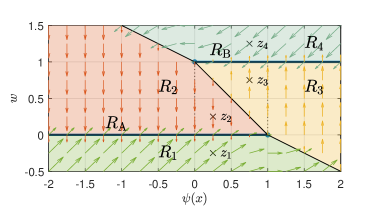
Figure 2: Illustration of the partitioning of the state space in $(\psi(x),w)$-plane for the time-freezing PSS via Voronoi regions with the corresponding auxiliary and DAE-forming dynamic’s vector fields. The Voronoi points $z_{i},i=1,\ldots,4$, are marked by the crosses.

Definition 1 (Auxiliary ODE).

The auxiliary ODE in regions $R_{2}$ and $R_{3}$ are denoted by $y^{\prime}=f_{\mathrm{aux},{\mathrm{A}}}(y)$ and $y^{\prime}=f_{\mathrm{aux},{\mathrm{B}}}(y)$, respectively. For every initial value $y(\tau_{\mathrm{s}})=y_{\mathrm{s}}$ such that $(w(\tau_{\mathrm{s}}),\psi(x(\tau_{\mathrm{s}}))=(1,0)$, for $y_{\mathrm{s}}\in{R}_{{\mathrm{B}}}$, (and $(w(\tau_{\mathrm{s}}),\psi(x(\tau_{\mathrm{s}}))=(0,1)$ for $y_{\mathrm{s}}\in{R}_{{\mathrm{A}}}$, respectively) and for every well-defined and finite time interval $\mathcal{T}_{\mathrm{jump}}\coloneqq(\tau_{\mathrm{s}},\tau_{\mathrm{r}})$ with the length $\tau_{\mathrm{jump}}\coloneqq\tau_{\mathrm{r}}-\tau_{\mathrm{s}}$, the auxiliary ODE satisfy the following properties: (i) $w(\tau)\in(0,1),\ \forall\tau\in\mathcal{T}_{\mathrm{jump}}$, (ii) $x(\tau_{\mathrm{s}})=x(\tau_{\mathrm{r}})$, and (iii) $w(\tau_{\mathrm{r}})=0$ (or $w(\tau_{\mathrm{r}})=1$).

In other words, we define an ODE whose trajectory endpoints on $\overline{\mathcal{T}}_{\mathrm{jump}}$ satisfy the state jump law associated with Eq. (4), cf. Fig. 2. The next proposition provides a constructive way to find an ODE with the above described properties.

Proposition 2 (Auxiliary ODE).

Given an initial value $y(\tau_{\mathrm{s}})=y_{\mathrm{s}}$ such that $w(\tau_{\mathrm{s}})=1$ and $\psi(x(\tau_{\mathrm{s}}))=0$, the ODE given by

$$y^{\prime}(\tau) =f_{\mathrm{aux},{\mathrm{A}}}(y)\coloneqq(\textbf{0}_{n_{x},1},-\gamma(\psi(x)-1),0),$$ (5)

where $\gamma:{\mathbb{R}}\to{\mathbb{R}}$ and $\gamma(x)=\frac{ax^{2}}{1+x^{2}}$ with $a>0$, is an auxiliary ODE defined in $R_{2}$. Similarly, for $y(\tau_{\mathrm{s}})=y_{\mathrm{s}}$ with $w(\tau_{\mathrm{s}})=0$ and $\psi(x(\tau_{\mathrm{s}}))=1$, the ODE

$$y^{\prime}(\tau) =f_{\mathrm{aux},{\mathrm{B}}}(y)\coloneqq(\textbf{0}_{n_{x},1},\gamma(\psi(x)),0).$$ (6)

is an auxiliary ODE in $R_{3}$. In both cases $\tau_{\mathrm{jump}}=\frac{1}{\gamma(-1)}$.

Proof. We prove the assertion for (5), since the second part follows similar lines. Since $x^{\prime}(\tau)=\textbf{0}_{n_{x},1}$ and $t^{\prime}(\tau)=0$ these two variables do not change their value, thus $\psi(x(\tau))=\psi(x(\tau_{\mathrm{s}}))=0$ and $t(\tau)=t(\tau_{\mathrm{s}})$ for $\tau\geq\tau_{\mathrm{s}}$. Hence, we have $w^{\prime}(\tau)=-\gamma(-1)<0$. By explicitly solving the ODE we obtain $w(\tau_{\mathrm{r}})=0$ for $\tau_{\mathrm{r}}=\tau_{\mathrm{s}}+\tau_{\mathrm{jump}}$, where $\tau_{\mathrm{jump}}=\frac{1}{\gamma(-1)}$. All conditions of Definition 1 are satisfied thus the proof is complete. ∎

We briefly discuss some of the proprieties of such an auxiliary ODE, since the are several ways to construct similar ODE. Loosely speaking, in Fig. 2 in $R_{2}$ the vector field should point in the negative $w$-detection and in $R_{3}$ in the positive $w$-direction, and be zero in all other directions. Note that for $\psi(x)\in(0,1)$ the vector fields of the auxiliary ODE in both cases point away from the manifold defined $\mathcal{M}=\{y\in{\mathbb{R}}^{n_{y}}\mid w+\psi(x)-1=0\}$. In such scenarios, there is usually locally no unique solution to the associated Filippov DI, as the trajectory can leave $\mathcal{M}$ at any point in time [16]. However, the system should never be initialized in this region, since this state is infeasible for the original system. We show later that it can never reach this undesired state if initialized appropriately. Furthermore, the auxiliary ODE from Proposition 2 have by construction the favorable property that they do not point away in both directions from $\mathcal{M}$ at the junction points $(0,1)$ and $(1,0)$. This is why the function $\gamma(\cdot)$ was introduced in the auxiliary ODE. Another favorable property is, if the system is initialized with the wrong value for $w(\cdot)$ for $\psi(x)\notin(0,1)$ the auxiliary ODE will automatically reinitialize $w(\cdot)$ while the physical time is frozen, cf. Fig 2.

We still need to define DAE-forming vector fields for the regions $R_{1}$ and $R_{4}$. These vector fields should be such that, together with the auxiliary dynamics in their respective regions, they results in sliding modes on $R_{{\mathrm{A}}}$ and $R_{{\mathrm{B}}}$ which match the dynamics of the initial system (4).

In a general PSS the vector fields are not defined on the region boundaries, thus we use Filippov’s convexification [16] as defined in Eq. (2), and denote the Filippov set associated to the time-freezing PSS by $F_{\mathrm{TF}}(\cdot)$. The next proposition gives a constructive way to find the desired vector fields.

Proposition 3 (DAE-forming ODE).

Suppose the regions $R_{2}$ and $R_{3}$ are equipped with the vector fields $f_{\mathrm{aux},{\mathrm{A}}}(\cdot)$ and $f_{\mathrm{aux},{\mathrm{B}}}(\cdot)$ from Proposition 2, respectively. Let the region $R_{1}$ be equipped with the ODE

$$y^{\prime} =f_{\mathrm{DF},{\mathrm{A}}}(y)\coloneqq 2(f_{{\mathrm{A}}}(x),0,1)-f_{\mathrm{aux},{\mathrm{A}}}(y),$$ (7)

then for $y\in R_{\mathrm{A}}$ it holds that $(f_{{\mathrm{A}}}(x),0,1)\in F_{\mathrm{TF}}(y)=\overline{\mathrm{conv}}\{f_{\mathrm{aux},{\mathrm{A}}}(y),f_{\mathrm{DF},{\mathrm{A}}}(y)\}$. Similarly, let the region $R_{4}$ be equipped with the following ODE

$$y^{\prime} =f_{\mathrm{DF},{\mathrm{B}}}(y)\coloneqq 2(f_{{\mathrm{B}}}(x),0,1)-f_{\mathrm{aux},{\mathrm{B}}}(y),$$ (8)

then for $y\in R_{\mathrm{B}}$ it holds that $(f_{{\mathrm{B}}}(x),0,1)\in F_{\mathrm{TF}}(y)=\overline{\mathrm{conv}}\{f_{\mathrm{aux},{\mathrm{B}}}(y),f_{\mathrm{DF},{\mathrm{B}}}(y)\}$.

Proof. We prove the assertion for Eq. (7) and the second part follows similar lines. Note that for $y\in R_{{\mathrm{A}}}=\{y\mid c(y)\coloneqq w=0,\psi(x)<1\}$ we have that $\nabla c(y)^{\top}f_{\mathrm{aux},{\mathrm{A}}}(y)<0$ and $\nabla c(y)^{\top}f_{\mathrm{DF},{\mathrm{A}}}(y)>0$. Hence, we have a sliding mode on $w=0$ with $\frac{\mathrm{d}w}{\mathrm{d}\tau}=0$ [16]. From (2) we have that $F_{\mathrm{TF}}(y)=\{\theta_{1}(2(f_{{\mathrm{A}}}(x),0,1)-f_{\mathrm{aux},{\mathrm{A}}}(y))+\theta_{2}f_{\mathrm{aux},{\mathrm{A}}}(y)\mid\theta_{1}+\theta_{2}=1,\theta_{1},\theta_{2}\geq 0\}$. From this relation and $w^{\prime}=0$ we obtain that $\theta_{1}-\theta_{2}=0$. Thus we can solve for $\theta_{1}$ and $\theta_{2}$, i.e., $\theta_{1}=\theta_{2}=\frac{1}{2}$, which yields $(f_{{\mathrm{A}}}(x),0,1)\in F_{\mathrm{TF}}(y)$. This completes the proof. ∎

Note that by construction the two sliding modes on $R_{\mathrm{A}}$ and $R_{\mathrm{B}}$ agree with the r.h.s. of Eq. (4) augmented by the dynamics of the clock state. Now we have defined vector fields in all regions of the time-freezing PSS which corresponds to the original system (4). Another favorable property of the chosen auxiliary and DAE forming ODE is: since $w^{\prime}(\tau)$ is bounded by $a>0$ it cannot make the sliding mode DAE arbitrarily stiff, especially if constraint drift happens.

3.2 A Tutorial Example

To illustrate the theoretical development we construct a time-freezing PSS for a thermostat system with hysteresis. The source code of the example is available in the repository of NOSNOC [15]. The system has a single state $x(\cdot)$ which models the temperature of a room which should stay inside the interval $x\in[18,20]$. As soon as the temperature drops below $x=18$ the heater is switched on and when the temperature grows above $x=20$ it is switched off. The two modes of operation are given by $\dot{x}=f_{{\mathrm{A}}}(x)=-0.2x+5$ when the heater is on and $\dot{x}=f_{{\mathrm{B}}}(x)=-0.2x$ when the heater is off. One can see that for $\psi(x)=0.5(x-18)$ we have a hybrid system that maches the finite automaton in Fig. 1(a).

Figure 3: Trajectories of the time-freezing PSS for a thermostat example in numerical time $\tau$ (left plot) and physical time $t$ (right plot).

For a time-freezing PSS we define the regions $R_{i}$ via the Voronoi points as in the last section. The auxiliary ODE’s r.h.s. according to Proposition 2 read as $f_{\mathrm{aux},{\mathrm{A}}}(y)=(0,-\gamma(0.5(x-18)-1),0)$ and $f_{\mathrm{aux},{\mathrm{B}}}(y)=(0,\gamma(0.5(x-18),0)$ with $a=1$. Similarly, the DAE-forming ODE r.h.s. according to Proposition 3 read as $f_{\mathrm{DF},{\mathrm{A}}}(y)=(-0.4x+10,\gamma(0.5(x-18)-1),2)$ and $f_{\mathrm{aux},{\mathrm{B}}}(y)=(-0.4x,-\gamma(0.5(x-18)),2)$.

We simulate now the time-freezing PSS with a FESD Radau-IIA integrator of order 3 [1] with $x(0)=15$ and $w(0)=0$. The left plot in Fig. 3 illustrates the evolution of the time-freezing PSS in numerical time. The red shaded areas indicate the phases when the auxiliary ODE is active with $w\notin\{0,1\}$ while the time is frozen, cf. bottom left plot. In the middle left plot we can see that $w(\tau)$ is now a continuous function in numerical time. The right plot in Fig. 3 shows the differential state in physical time $t(\tau)$. Clearly, in the middle right plot $w(t(\tau))$ is now a discontinuous function, hence the state jumps are successfully recovered in physical time.

4 Solution Equivalence

From the developments in the last section, the solution equivalence is nearly apparent. We formalize it in the next theorem.

Theorem 4.

Regard the IVP corresponding to: (i) the Filippov DI of the time-freezing PSS equipped with the vector fields from Proposition 2 and 3 with a initial value $y(0)=(z_{0},0)$ with $z_{0}=(x_{0},w_{0})$ and $w_{0}\in\{0,1\}$, on a time interval $[0,\tau_{\mathrm{f}}]$, (ii) the ODE with state jumps from Eq. (4) with $z(0)=z_{0}$ on a time interval $[0,t_{\mathrm{f}}]=[0,t(\tau_{\mathrm{f}})]$. Suppose solutions exist to both IVP.

Then the solutions of the two IVPs $z(t;z_{0})$ and $y(\tau;y_{0})$ fulfill at any $\dfrac{dt}{d\tau}=t^{\prime}(\tau)\neq 0$:

$$z(t(\tau);z_{0}) =\!My(t(\tau);y_{0}),\!\text{ with }\!M\!\!=\!\begin{bmatrix}I_{n_{x}+1}\!\!\!&\!\!\!\textbf{0}_{n_{x}+1,1}\end{bmatrix}\!\!.$$ (9)

Proof. Denote the solution of IVP (i) by $y_{1}(\tau;y_{0})$ for $\tau\in(0,\hat{\tau})$ and for (ii) and $t(\tau)\in(0,t(\hat{\tau}))$ by $z_{1}(t(\tau);z_{0})$. For a given $w(0)=0$ (or $1$) we have from Proposition 3 that $y^{\prime}=(f_{\mathrm{A}}(x),0,1)$ (or $y^{\prime}=(f_{\mathrm{B}}(x),0,1)$). Note that if there is no $\tau_{\mathrm{s}}\in(0,\hat{\tau})$ for the IVP (i) such that an auxiliary ODE becomes active, then $t(\tau)=\int_{0}^{\tau}\mathrm{d}\tau_{1}=\tau$. Since $(f_{\mathrm{A}}(x),0)=M(f_{\mathrm{A}}(x),0,1)$, $(f_{\mathrm{B}}(x),0)=M(f_{\mathrm{B}}(x),0,1)$ and $z_{0}=My_{0}$ by setting $\hat{\tau}=\tau_{\textrm{f}}$, it follows that (9) holds.

Suppose now that we have a $\tau_{\mathrm{s}}\in(0,\tau_{\mathrm{f}})$ such that for $w(\tau_{\mathrm{s}})=1$ the auxiliary ODE $y^{\prime}=f_{\mathrm{aux},{\mathrm{A}}}(y)$ becomes active (or similarly for $w(\tau_{\mathrm{s}})=0$, $y^{\prime}=f_{\mathrm{aux},{\mathrm{B}}}(y)$ becomes active). From the first part of the proof we have that (9) holds for $\tau\in(0,\tau_{\textrm{s}})$ and hence for all $t(\tau)\in(0,t_{\mathrm{s}}^{-})$, where $t_{\mathrm{s}}^{-}=t(\tau_{\mathrm{s}})$. From Proposition 2 we have that the solution satisfies $x(\tau_{\mathrm{s}})=x(\tau_{\mathrm{r}})$ and $w(\tau_{\mathrm{r}})=0$ (or $w(\tau_{\mathrm{r}})=1$) with $t^{\prime}(\tau)=0$ for $\tau\in[\tau_{\mathrm{s}},\tau_{\mathrm{r}}]$. Hence, we have also $t(\tau_{\textrm{r}})=t_{\mathrm{s}}^{+}=t(\tau_{\textrm{s}})$. Denote by $y_{\mathrm{s}}=(x(\tau_{\mathrm{r}}),w(\tau_{\mathrm{r}}),t(\tau_{\mathrm{r}}))$. Using this we have $y_{1}(\tau-\tau_{\textrm{r}},y_{\mathrm{s}})=y(\tau,y_{0})$ for $\tau\in(\tau_{\textrm{r}},\tilde{\tau})$ and denoting $z_{\mathrm{s}}=My_{\mathrm{s}}$ we see that $z_{1}(t(\tau)-t_{s};z_{\mathrm{s}})=x(t(\tau),z_{0})$ for $t(\tau)\in(t_{s}^{+},\tilde{\tau})$. Assume that a single activation of an auxiliary ODE takes place and set $\tilde{\tau}=\tau_{\mathrm{f}}$. Since the intervals $(t_{s},t_{\textrm{f}})$ and $(\tau_{\textrm{r}},\tau_{\textrm{f}})$ have the same length and $z_{\mathrm{s}}=My_{\mathrm{s}}$ from the definitions of the corresponding IVP, we conclude that relation (9) holds. If the auxiliary ODE becomes active multiple times we simply apply the same argument on the corresponding sub-intervals. This completes the proof. ∎

The last theorem opens the door to study the regarded hybrid system with hysteresis as a Filippov system and to apply their rich theory e.g., solution existence results [16]. From the practical side, we can use numerical methods for Filippov systems which allows us to avoid the use of integer variables.

5 Numerical Example: Time Optimal Problem of a Car with Turbo Charger

In this section we apply the theoretical developments in a numerical example of a time optimal control problem of a car with turbo from [9]. We consider a double-integrator car model equipped with a turbo accelerator which follows a hysteresis characteristic as in Fig. 1(b). This makes the seemingly simple model severely nonlinear and nonsmooth.

The car is described by its position $q(t)$, velocity $v(t)$ and turbo charger state $w(t)\in\{0,1\}$. The control variable is the car acceleration $u(t)$. The turbo accelerator is activated when the velocity exceeds $v\geq 15$ and is deactivated when it falls below $v\leq 10$. When it is on, it makes the nominal acceleration $u(t)$ three times greater. One can see that $\psi(x)=\frac{v-10}{5}$. In summary, the state vector reads as $z=(q,v,w)\in{\mathbb{R}}^{3}$ with two modes of operation described by $f_{{\mathrm{A}}}(z)=(v,u,0)$ and $f_{{\mathrm{B}}}(z)=(v,3u,0)$. The acceleration is bounded by $|u|\leq\bar{u}$, $\bar{u}=5$ and the velocity by $|v|\leq\bar{v}$, $\bar{v}=25$.

In the OCP we consider the time-freezing PSS associated to the car model on a numerical time interval $\tau\in[0,\tau_{\mathrm{f}}]$. The car should reach the goal $q(t(\tau_{\mathrm{f}}))\!=q_{\mathrm{f}}\!=150$ with $v(t(\tau_{\mathrm{f}}))\!=v_{\mathrm{f}}\!=0$, whereby $z(0)=z_{0}=\textbf{0}_{3,1}$. The auxiliary and DAE-forming dynamics are chosen according to Propositions 2 (with $a=1$) and 3, respectively. The OCP reads as:

$$\min_{y(\cdot),u(\cdot),s(\cdot)}\quad t(\tau_{\mathrm{f}})$$ (10a)

s.t. $$y(0)=(z_{0},0),$$ (10b)

$${y}^{\prime}(\tau)\!\in\!s(\tau)\!F_{\mathrm{TF}}(y(\tau),\!u(\tau)),\!\;\tau\in\![0,\tau_{\mathrm{f}}],$$ (10c)

$$-\bar{u}\leq u(\tau)\leq\bar{u},\;\tau\in[0,\tau_{\mathrm{f}}],$$ (10d)

$$\bar{s}^{-1}\leq s(\tau)\leq\bar{s},\;\tau\in[0,\tau_{\mathrm{f}}],$$ (10e)

$$-\bar{v}\leq v(\tau)\leq\bar{v},\;\tau\in[0,\tau_{\mathrm{f}}],$$ (10f)

$$(q(\tau_{\mathrm{f}}),v(\tau_{\mathrm{f}}))=(q_{\mathrm{f}},v_{\mathrm{f}}).$$ (10g)

The objective consist of minimizing the final physical time. Since a time optimal control problem is considered, we introduce the scalar speed-of-time control variable $s(\cdot)$ which introduces a time-transformation and enables to have a variable terminal physical time $T_{\mathrm{f}}=t(\tau_{\mathrm{f}})$. It is bounded by (10e) with $\bar{s}=10$. NOSNOC ensures equidistant control grids in numerical and physical time $\tau$.

The OCP is discretized with a FESD Radau-IIA scheme of order 3 with $N=10$ control intervals and $N_{\mathrm{fe}}=3$ additional integration steps on every control interval, with $\tau_{\mathrm{f}}=5$. The controls are taken to be piecewise constant over the control intervals. The OCP discretization and MPCC homotopy is carried out via the open source tool NOSNOC, which has IPOPT [18] and CasADi [19] as a back-end.

Additionally, we compare our approach to the mixed integer formulation of [9]. We take the same control and state discretization as in NOSNOC which results $56$ binary variables. Switches in the integer formulation are allowed only at the control interval boundaries, as a switch detection formulation requires significantly more integer variables and introduces more nonlinearity.

The problem is solved with the dedicated mixed integer nonlinear programming (MINLP) solver Bonmin [20]. Note that the only nonlinearity in the MINLP is due to the time-transformation for the optimal time $T_{\mathrm{f}}$. Therefore, in a second experiment we fix $T_{\mathrm{f}}$ and solve the resulting MILP with the commercial solver Gurobi. We make a bisection-type search in $T_{\mathrm{f}}$. The MILP with the smallest $T_{\mathrm{f}}$ that is still feasible, delivers the optimal time $T_{\mathrm{f}}$. In this experiment 22 MILP were solved for an accuracy of $10^{-6}$. To determine the solution quality, we additionally perform a high accuracy solution with the computed optimal controls and obtain $x_{\mathrm{sim}}(t)$. We compare the terminal constraint satisfactions: $E(T_{\mathrm{f}})=\|x_{\mathrm{sim}}(T_{\mathrm{f}})-(q_{\mathrm{f}},v_{\mathrm{f}})\|_{2}$. The source core for the simulation and the two MIOP approaches are provided in the NOSNOC repository [15].

The results are summarized in Table 1. All three approaches provide a similar objective value. Gurobi is the fastest solver, NOSNOC is only slightly slower and Bonmin is significantly slower. The smallest terminal error is achieved via NOSNOC. This is due to the underlying FESD discretization, cf. [1]. Gurobi and Bonmin have the same discretization without switch detection and result in the same terminal error. On the other hand, Gurobi provides the most robust approach, as NOSNOC (i.e., IPOPT as underlying NLP solver) fails to converge in some variations of the discretization.

Figure 4: Solutions of the OCP (10) in physical time. The top left and right plots show the velocity $v(t)$ and optimal controls $u(t)$, respectively. The bottom left and right plots show the hysteresis state $w(t)$ and the solution trajectory in the $(v,w)$-plane, respectively.

The results computed by NOSNOC is depicted in Fig. 4. One can see an intuitive behavior as the car uses the turbo accelerator as much as possible to reach the goal time optimally, with $T_{\mathrm{f}}=10.26$.

6 Conclusion

In this paper we introduced a novel time-freezing reformulation for a class of hybrid systems with hysteresis. It transforms the systems with state jumps into PSS for which we leverage the recently developed FESD method which enables high accuracy optimal control by solving only smooth NLP. Thus, we can avoid use of computationally expensive mixed integer strategies in numerical optimal control and obtain quickly good and accurate nonsmooth solutions. In the theoretical part, constructive ways to find auxiliary and DAE-forming ODE are provided and solution equivalence is proven. In future time-freezing for other types of finite automaton and hysteresis systems, as e.g., described in the introduction should be investigated as well.

Table 1: Comparison of NOSNOC to mixed integer formulations.

Solver	$T_{\mathrm{f}}$	CPU Time [s]	$E(T_{\mathrm{f}})$
NOSNOC	10.26	8.87	9.49e-02
Gurobi with bisection	11.21	5.31	7.88e+01
Bonmin	11.28	1481.58	7.88e+01

References

- [1] A. Nurkanović, M. Sperl, S. Albrecht, and M. Diehl, “Finite Elements with Switch Detection for Direct Optimal Control of Nonsmooth Systems,” to be submitted, 2022.
- [2] A. Visintin, Differential models of hysteresis. Springer-Verlag, Berlin, 1994, vol. Appl. Math. Sci. 111.
- [3] J. Lunze and F. Lamnabhi-Lagarrigue, Handbook of hybrid systems control: theory, tools, applications. Cambridge University Press, 2009.
- [4] B. Brogliato and A. Tanwani, “Dynamical systems coupled with monotone set-valued operators: Formalisms, applications, well-posedness, and stability,” SIAM Review, vol. 62, no. 1, pp. 3–129, 2020.
- [5] L. Vandenberghe, B. De Moor, and J. Vandewalle, “The generalized linear complementarity problem applied to the complete analysis of resistive piecewise-linear circuits,” IEEE transactions on circuits and systems, vol. 36, no. 11, pp. 1382–1391, 1989.
- [6] F. Ceragioli, C. De Persis, and P. Frasca, “Discontinuities and hysteresis in quantized average consensus,” Automatica, vol. 47, no. 9, pp. 1916–1928, 2011.
- [7] F. Bagagiolo and R. Maggistro, “Hybrid thermostatic approximations of junctions for some optimal control problems on networks,” SIAM Journal on Control and Optimization, vol. 57, no. 4, pp. 2415–2442, 2019.
- [8] A. Bemporad and M. Morari, “Control of systems integrating logic, dynamics, and constraints,” Automatica, vol. 35, no. 3, pp. 407–427, 1999.
- [9] M. Avraam, “Modelling and optimisation of hybrid dynamic processes.” Ph.D. dissertation, Imperial College London (University of London), 2000.
- [10] A. Nurkanović, S. Albrecht, and M. Diehl, “Limits of MPCC Formulations in Direct Optimal Control with Nonsmooth Differential Equations,” in 2020 European Control Conference (ECC), 2020, pp. 2015–2020.
- [11] D. E. Stewart and M. Anitescu, “Optimal control of systems with discontinuous differential equations,” Numerische Mathematik, vol. 114, no. 4, pp. 653–695, 2010.
- [12] A. Nurkanović, T. Sartor, S. Albrecht, and M. Diehl, “A Time-Freezing Approach for Numerical Optimal Control of Nonsmooth Differential Equations with State Jumps,” IEEE Control Systems Letters, vol. 5, no. 2, pp. 439–444, 2021.
- [13] A. Nurkanović, S. Albrecht, B. Brogliato, and M. Diehl, “The Time-Freezing Reformulation for Numerical Optimal Control of Complementarity Lagrangian Systems with State Jumps,” arXiv preprint, 2021.
- [14] A. Nurkanović and M. Diehl, “NOSNOC: A software package for numerical optimal control of nonsmooth systems,” Submitted to The IEEE Control Systems Letters (L-CSS), 2022.
- [15] “NOSNOC,” https://github.com/nurkanovic/nosnoc, 2022.
- [16] A. F. Filippov, Differential Equations with Discontinuous Righthand Sides. Springer Science & Business Media, Series: Mathematics and its Applications (MASS), 2013, vol. 18.
- [17] M. Anitescu, P. Tseng, and S. J. Wright, “Elastic-mode algorithms for mathematical programs with equilibrium constraints: global convergence and stationarity properties,” Mathematical Programming, vol. 110, no. 2, pp. 337–371, 2007.
- [18] A. Wächter and L. T. Biegler, “On the implementation of an interior-point filter line-search algorithm for large-scale nonlinear programming,” Mathematical Programming, vol. 106, no. 1, pp. 25–57, 2006.
- [19] J. A. E. Andersson, J. Gillis, G. Horn, J. B. Rawlings, and M. Diehl, “CasADi – a software framework for nonlinear optimization and optimal control,” Mathematical Programming Computation, vol. 11, no. 1, pp. 1–36, 2019.
- [20] P. Bonami, L. T. Biegler, A. R. Conn, G. Cornuéjols, I. E. Grossmann, C. D. Laird, J. Lee, A. Lodi, F. Margot, N. Sawaya et al., “An algorithmic framework for convex mixed integer nonlinear programs,” Discrete optimization, vol. 5, no. 2, pp. 186–204, 2008.