Primordial helium-3 redux: The helium isotope ratio of the Orion nebula

Abstract

We report the first direct measurement of the helium isotope ratio, ³He/⁴He, outside of the Local Interstellar Cloud, as part of science verification observations with the upgraded CRyogenic InfraRed Echelle Spectrograph (CRIRES). Our determination of ³He/⁴He is based on metastable He i* absorption along the line-of-sight towards $\Theta^{2}$A Ori in the Orion Nebula. We measure a value ³He/⁴He $=(1.77\pm 0.13)\times 10^{-4}$, which is just $\sim 40$ per cent above the primordial relative abundance of these isotopes, assuming the Standard Model of particle physics and cosmology, (³He/⁴He)${}_{\rm p}=(1.257\pm 0.017)\times 10^{-4}$. We calculate a suite of galactic chemical evolution simulations to study the Galactic build up of these isotopes, using the yields from Limongi & Chieffi (2018) for stars in the mass range $M=8-100~{}{\rm M}_{\odot}$ and Lagarde et al. (2011, 2012) for $M=0.8-8~{}{\rm M}_{\odot}$. We find that these simulations simultaneously reproduce the Orion and protosolar ³He/⁴He values if the calculations are initialized with a primordial ratio $(^{3}{\rm He}/^{4}{\rm He})_{\rm p}=(1.043\pm 0.089)\times 10^{-4}$. Even though the quoted error does not include the model uncertainty, this determination agrees with the Standard Model value to within $\sim 2\sigma$. We also use the present-day Galactic abundance of deuterium (D/H), helium (He/H), and ³He/⁴He to infer an empirical limit on the primordial ³He abundance, $(^{3}{\rm He/H})_{\rm p}\leq(1.09\pm 0.18)\times 10^{-5}$, which also agrees with the Standard Model value. We point out that it is becoming increasingly difficult to explain the discrepant primordial ⁷Li/H abundance with non-standard physics, without breaking the remarkable simultaneous agreement of three primordial element ratios (D/H, ⁴He/H, and ³He/⁴He) with the Standard Model values.

1 Introduction

Most of the baryonic matter in the Universe was made within a few minutes following the Big Bang. This brief period of element genesis is commonly referred to as Big Bang Nucleosynthesis (BBN), and was primarily responsible for making the isotopes of the lightest chemical elements (for a review of this topic, see Cyburt et al. 2016; Pitrou et al. 2018; Fields et al. 2020). The relative abundances of these elements are sensitive to the physical conditions and content of the Universe during the first few minutes. Thus, by measuring the relative abundances of the light elements made during BBN, we can learn about the physics of the very early Universe.

The abundances of the BBN nuclides are traditionally calculated and measured relative to the number of hydrogen atoms. Most studies have focused on determining the abundances of deuterium (D/H), helium-3 (³He/H), helium-4 (⁴He/H), and lithium-7 (⁷Li/H). Current measures of the primordial D/H and ⁴He/H abundances broadly agree with the values calculated assuming the Standard Model of particle physics and cosmology (Izotov et al. 2014; Cooke et al. 2018; Fernández et al. 2019; Hsyu et al. 2020; Aver et al. 2021; Valerdi et al. 2021; Kurichin et al. 2022). However, the ⁷Li/H abundance inferred from the atmospheres of the most metal-poor halo stars deviates from the Standard Model value by $\sim 6\sigma$ (Asplund et al. 2006; Aoki et al. 2009; Meléndez et al. 2010; Sbordone et al. 2010; Matas Pinto et al. 2021). At present, it is still unclear if the stellar atmospheres of metal-poor stars have burnt some of the lithium (Korn et al., 2006; Lind et al., 2009), or if an ingredient is missing from the Standard Model (for a comprehensive review on this topic, see Fields 2011).

The primordial abundance of ³He has received relatively less attention, largely because it is so challenging to measure; for almost all of the helium atomic transitions, ⁴He swamps ³He because it is $\sim 10,000$ times more abundant and the isotope shifts of almost all transitions are $\lesssim 15\,{\rm km~{}s}^{-1}$. However, because ³He has a non-zero nuclear spin, the ground state of ³He exhibits hyperfine structure, which gives rise to a ³He⁺ spin-flip transition at $8.7\,{\rm GHz}$ — while ⁴He does not. This transition has enabled the only measurement of the ³He/H abundance outside of the Solar System (Bania et al., 2002), and has only been detected towards H ii regions in the Milky Way (Balser & Bania, 2018). Based on these observations, there appears to be a gentle decrease of ³He/H with increasing galactocentric radius, in line with models of galactic chemical evolution (Lagarde et al., 2012). The best available estimate of the ³He/H ratio of the outer Milky Way is ³He/H $=(1.10\pm 0.28)\times 10^{-5}$, which is solely based on the most distant and well-characterized H ii region (S209) where the He⁺ 8.7 GHz line has been detected (Balser & Bania, 2018). Unfortunately, measurements of the Milky Way ³He abundance may not represent the primordial value due to post-BBN production of ³He; future measurements of this isotope in near-pristine environments are required to understand the complete cosmic chemical evolution of ³He, and to secure its primordial abundance.

While the abundance of ³He is challenging to measure, there are several proposed approaches that may secure a measurement of the primordial ³He abundance with future facilities. Akin to the detection of ³He⁺ $8.7~{}{\rm GHz}$ in Galactic H ii regions, it may be possible (but extremely challenging) to detect ³He⁺ emission around growing supermassive black holes at redshift $z>12$ (Vasiliev et al., 2019), provided that the quasar environment retains a primordial composition. Another possibility is to detect the ³He⁺ $8.7~{}{\rm GHz}$ transition in absorption against the spectrum of a radio bright quasar during helium reionization (at redshift $z\sim 3$; McQuinn & Switzer 2009; Takeuchi et al. 2014; Khullar et al. 2020). One advantage of this approach is that the gas in the intergalactic medium is largely unprocessed, and the ³He/H value would therefore closely reflect the primordial value. The intergalactic medium is also somewhat simpler to model than the Galactic H ii regions where this ³He⁺ transition has previously been studied in emission.

An alternative approach proposed by Cooke (2015) is to use a combination of optical and near-infrared transitions to measure the helium isotope ratio (³He/⁴He). Because the ionization potential of ³He is almost identical to that of ⁴He, the helium isotope ratio is much less sensitive to ionization corrections than ³He/H. Furthermore, Cooke (2015) highlighted that the helium isotope ratio and D/H provide orthogonal bounds on the present day baryon density ($\Omega_{\rm B,0}\,h^{2}$) and the effective number of neutrino species ($N_{\rm eff}$). Finally, the isotope shifts of the optical and near-infrared transitions are all different, so a relative comparison of any two line profiles would allow one to unambiguously identify ³He.

The only available measures of the helium isotope ratio are based on terrestrial and Solar System environments, including the Earth’s mantle (³He/⁴He $=[1.1-4.2]\times 10^{-5}$; Péron et al. 2018), meteorites (³He/⁴He $=[1.47-190]\times 10^{-4}$; Busemann et al. 2000; Krietsch et al. 2021), the Local Interstellar Cloud (³He/⁴He $=1.62\pm 0.29\times 10^{-4}$; Busemann et al. 2006), Jupiter (³He/⁴He $=1.66\pm 0.05\times 10^{-4}$; Mahaffy et al. 1998), and solar wind particles (³He/⁴He $=[4.5-4.8]\times 10^{-4}$; Heber et al. 2012). The elevated values measured from the present day solar wind reflect the burning of deuterium into ³He during the pre-main-sequence evolution of the Sun. Therefore, the ³He/⁴He measure based on Jupiter is our best estimate of the proto-solar value of the helium isotope ratio.

In this paper we propose a new approach, qualitatively similar to that described by Cooke (2015), to measure the helium isotope ratio. Using this approach, we report the first direct measurement of ³He/⁴He beyond the Local Interstellar Cloud. Our approach uses the light of a background object (in our case, a bright O star) to study the absorbing material along the line-of-sight. Since all ground state (singlet) transitions of neutral helium are in the far ultraviolet (see e.g. Cooke & Fumagalli 2018), the only helium absorption lines accessible to ground-based telescopes arise from excited states of metastable helium (He i*), which has a lifetime of $\sim 130~{}$min.

Interstellar absorption lines due to metastable helium were first identified toward the Orion Nebula nearly a century ago (Wilson, 1937). They have since been detected towards five stars associated with the Orion Nebula (O’dell et al., 1993; Oudmaijer et al., 1997), towards several stars in the young open cluster NGC 6611 (Evans et al., 2005), and towards $\zeta$ Oph (Galazutdinov & Krelowski, 2012). Extragalactic He i* absorption lines have also been detected in the host galaxy of the gamma-ray burst GRB 140506A at redshift $z=0.889$ (Fynbo et al., 2014). Several broad absorption line quasars also exhibit He i* absorption, although the kinematics of these features are significantly broader ($\sim 1000\,{\rm km~{}s}^{-1}$; Liu et al. 2015) and more complicated than the interstellar features ($\sim 10\,{\rm km~{}s}^{-1}$). The interstellar He i* absorption profiles tend to be quiescent and smooth, suggesting that a very simple broadening mechanism is responsible for the line shape, and the absorbing gas is homogeneous. Furthermore, given the lifetime of the metastable state and the fact that metastable helium only occurs in regions where He⁺ is recombining, the He i* absorption likely occurs at the edge of the He ii ionization region around the hottest stars.

The simplicity and quiescence ($\lesssim 10~{}{\rm km~{}s}^{-1}$) of the line profiles is one of the key benefits of using He i* absorption to measure the helium isotope ratio. Demonstrating the promise of this new approach for measuring the primordial ³He/⁴He ratio is the primary motivation of this work. In Section 2 we provide the details of our CRIRES Science Verification observations. The atomic data are described in Section 3 and our absorption line profile analysis is presented in Section 4. We discuss the implications of our measurement in Section 5 before summarizing our conclusions in Section 6.

2 Observations

Motivated by the strong, kinematically quiescent He i* absorption towards $\Theta^{2}$A Ori (O’dell et al., 1993), we obtained Very Large Telescope (VLT) CRyogenic InfraRed Echelle Spectrograph (CRIRES; Kaeufl et al. 2004) observations of $\Theta^{2}$A Ori as part of the CRIRES Upgrade Project (Dorn et al., 2014) science verification on 2021 Sep 18. CRIRES is an infrared cross-dispersed echelle spectrograph covering a wavelength range from 0.95 to 5.3 $\mu$m at a spectral resolving power $R\simeq 40,000$ or $R\simeq 80,000$. As part of the upgrade, a cross-disperser was installed to increase the simultaneously covered wavelength range by a factor of ten, and three sensitive Hawaii 2RG detectors were installed. CRIRES is based at the Nasmyth focus of UT3, and is fed by the Multi-Applications Curvature Adaptive Optics (MACAO) system.

2.1 CRIRES data

The goal of our observations is to detect the ³He i* $\lambda 1.0833\,\mu$m absorption line to obtain the first direct measure of the helium isotope ratio beyond the Local Interstellar Cloud. Detecting ³He i* absorption is challenging, as we expect the ³He i* absorption line to be very weak, and only detectable in spectra of both high resolution ($R\gtrsim 40,000$) and very high signal-to-noise ratio (${\rm S/N}>1000$). To minimise the effect of pixel-to-pixel sensitivity variations affecting the final combined S/N, we designed the observing programme to ensure that the target spectrum was projected onto different detector pixels with each exposure. A total of ten exposures were acquired at two nodding positions (20 exposures total); each nod was separated by $7.5^{\prime\prime}$, and the target spectrum was shifted by $0.5^{\prime\prime}$ on the detector with each exposure. To minimize the effects of non-linearity, the detector integration time was DIT=5 s, and each exposure contains NDIT=20 detector integrations, resulting in an exposure time of 100 s. We also took four shorter exposures; two with NDIT=3 and two with NDIT=1. Therefore, the total integration time on source was 2040 s. We used the $0.2^{\prime\prime}$ slit in combination with the Multi-Applications Curvature Adaptive Optics (MACAO) system. The nominal spectral resolving power of this setup is $R\sim 80,000$.

The data were reduced using a set of custom-built routines in combination with the PypeIt data reduction pipeline (Prochaska et al., 2020). A combination of nine flatfield frames were used to remove the pixel-to-pixel sensitivity variations. We subtracted a pair of science frames at different nod positions to remove the periodic CRIRES detector pattern, hot pixels, and any background emission (see Figure 1). Bad pixels were identified and masked, and the object was traced and optimally extracted using PypeIt. A spectrum of the background emission (i.e. the sky and H ii region emission) was also extracted from the individual science frames (i.e. without subtracting observations at different nod positions), and used for validation (see Section 4.2).

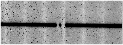
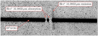
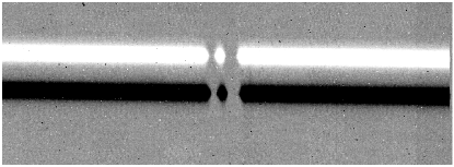
Figure 1: An example of a raw CRIRES frame (top), after detector pattern removal (middle), and after differencing a pair of science frames at different nod positions (bottom). These panels show the He i* absorption superimposed on the spectrum of $\Theta^{2}$A Ori. Wavelength increases from left to right. Faint He i* emission is detected in the red wing of the line profile (see middle panel). Since the emission only appears in the red wing, it presumably arises at the edge of an expanding shell. The ‘pepper’ that can be seen in the top two frames is due to hot pixels, that are largely removed as part of differencing (see bottom panel).

The wavelength calibration was performed using a second order polynomial fit to the telluric absorption lines imprinted on the target spectrum (see Seifahrt et al. 2010). Due to the low line density (six telluric lines spanning 2048 pixels) and the weakness of these features, the solution was not sufficiently accurate given the high S/N desired. We therefore used the telluric solution as a first guess, and performed a simultaneous fit to all individual exposures to construct a model of the continuum, absorption, and wavelength solution (see Section 2.1 for details of the line fitting procedure). The wavelength correction comprised a simple shift and stretch to the telluric wavelength solution, using as a reference archival optical observations of He i* $\lambda 3188$ Å (described in Section 2.2). The continuum was modelled with a global high order Legendre polynomial for all exposures, combined with a multiplicative scale and tilt to account for the relative sensitivity of each exposure. Deviant pixels were masked during the fitting. We applied the wavelength and continuum corrections to each extracted spectrum, resampled all exposures onto a single wavelength scale, and combined all exposures while sigma-clipping (a rejection threshold of $3\sigma$).

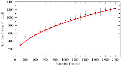
Figure 2: The increase of the final combined S/N as the exposure time is increased. The black points with error bars are based on randomly combining exposures of a set total exposure time, where the error bar represents the dispersion. The red curve shows the expected relation, where the signal-to-noise ratio is proportional to the square root of the exposure time. Note that each data point is not independent.

The inferred error spectrum is dominated by the photon count uncertainty of the target spectrum. However, this does not include additional noise terms that arise due to instrument and data reduction systematics (e.g. residual pixel-to-pixel sensitivity variations, wavelength/continuum calibration, etc.). To uniformly account for unknown systematic uncertainties, we fit a low order Legendre polynomial to the target continuum, calculate the observed deviations about this model, and scale the error spectrum so that it represents more faithfully the observed fluctuations of the data. From these fluctuations, we measure a S/N=1260 per $1.5~{}{\rm km~{}s}^{-1}$ pixel, based on the blue-side continuum near the He i* $\lambda 1.0833\,\mu$m absorption line. To test if the S/N we achieve is limited by data reduction systematics, we combined a random subset of $n$ exposures to determine how the S/N increases as the total exposure time increases. We repeated this process 100 times for $n=1,2\ldots 20$; the mean values and dispersions for each $n$ (recall, each exposure time is 100 s) are shown as the black points with error bars in Figure 2. The expected growth of the S/N, assuming it increases as the square root of the exposure time, is shown as the red curve. The good agreement between the data and the expected growth suggests that the S/N is currently limited by exposure time, and not data reduction systematics.

2.2 UVES data

We supplemented our CRIRES observations of $\Theta^{2}$A Ori with archival VLT Ultraviolet and Visual Echelle Spectrograph (UVES) observations of this target, acquired on 2014 September 24 (Programme ID: 194.C-0833). These data were acquired as part of the ESO Diffuse Interstellar Bands Large Exploration Survey (EDIBLES); for further details about the instrument setup and data reduction, see Cox et al. (2017). The nominal spectral resolution of these data are $R\simeq 71050$, and cover the He i* transitions at $3188\,$Å and $3889\,$Å.

3 Atomic Data

Table 1: Atomic data of the He i* triplet transitions used in this work.

Ion	Lower State	Upper State	$F$	$F^{\prime}$	$\lambda_{0}$	$f$	$\gamma_{ul}$	$\Delta v_{3-4}$
					(Å)		$(10^{7}~{}{\rm s}^{-1})$	(km s-1)
3He i∗	1s2s ${}^{3}{\rm S}_{1}$	1s2p ${}^{3}{\rm P}^{\rm o}_{0}$	1.5	0.5	10833.27471	0.03996	1.022	+33.7
3He i∗	1s2s ${}^{3}{\rm S}_{1}$	1s2p ${}^{3}{\rm P}^{\rm o}_{0}$	0.5	0.5	10833.53856	0.01998	1.022	+41.0
3He i∗	1s2s ${}^{3}{\rm S}_{1}$	1s2p ${}^{3}{\rm P}^{\rm o}_{1}$	1.5	1.5	10834.55125	0.09989	1.022	+36.9
3He i∗	1s2s ${}^{3}{\rm S}_{1}$	1s2p ${}^{3}{\rm P}^{\rm o}_{1}$	0.5	1.5	10834.81516	0.01998	1.022	+44.2
3He i∗	1s2s ${}^{3}{\rm S}_{1}$	1s2p ${}^{3}{\rm P}^{\rm o}_{1}$	1.5	0.5	10834.37457	0.01998	1.022	+32.0
3He i∗	1s2s ${}^{3}{\rm S}_{1}$	1s2p ${}^{3}{\rm P}^{\rm o}_{1}$	0.5	0.5	10834.63847	0.03996	1.022	+39.3
3He i∗	1s2s ${}^{3}{\rm S}_{1}$	1s2p ${}^{3}{\rm P}^{\rm o}_{2}$	1.5	2.5	10834.62099	0.17980	1.022	+36.4
3He i∗	1s2s ${}^{3}{\rm S}_{1}$	1s2p ${}^{3}{\rm P}^{\rm o}_{2}$	1.5	1.5	10834.34842	0.01998	1.022	+28.8
3He i∗	1s2s ${}^{3}{\rm S}_{1}$	1s2p ${}^{3}{\rm P}^{\rm o}_{2}$	0.5	1.5	10834.61232	0.09989	1.022	+36.1
3He i∗	1s2s ${}^{3}{\rm S}_{1}$	1s3p ${}^{3}{\rm P}^{\rm o}_{0}$	1.5	0.5	3889.90165	0.00478	1.055	+15.0
3He i∗	1s2s ${}^{3}{\rm S}_{1}$	1s3p ${}^{3}{\rm P}^{\rm o}_{0}$	0.5	0.5	3889.93567	0.00239	1.055	+17.7
3He i∗	1s2s ${}^{3}{\rm S}_{1}$	1s3p ${}^{3}{\rm P}^{\rm o}_{1}$	1.5	1.5	3889.93000	0.01194	1.055	+14.1
3He i∗	1s2s ${}^{3}{\rm S}_{1}$	1s3p ${}^{3}{\rm P}^{\rm o}_{1}$	0.5	1.5	3889.96402	0.00239	1.055	+16.7
3He i∗	1s2s ${}^{3}{\rm S}_{1}$	1s3p ${}^{3}{\rm P}^{\rm o}_{1}$	1.5	0.5	3889.94461	0.00239	1.055	+15.2
3He i∗	1s2s ${}^{3}{\rm S}_{1}$	1s3p ${}^{3}{\rm P}^{\rm o}_{1}$	0.5	0.5	3889.97863	0.00478	1.055	+17.8
3He i∗	1s2s ${}^{3}{\rm S}_{1}$	1s3p ${}^{3}{\rm P}^{\rm o}_{2}$	1.5	2.5	3889.96332	0.02149	1.055	+16.4
3He i∗	1s2s ${}^{3}{\rm S}_{1}$	1s3p ${}^{3}{\rm P}^{\rm o}_{2}$	1.5	1.5	3889.96058	0.00239	1.055	+16.2
3He i∗	1s2s ${}^{3}{\rm S}_{1}$	1s3p ${}^{3}{\rm P}^{\rm o}_{2}$	0.5	1.5	3889.99460	0.01194	1.055	+18.8
3He i∗	1s2s ${}^{3}{\rm S}_{1}$	1s4p ${}^{3}{\rm P}^{\rm o}_{0}$	1.5	0.5	3188.79672	0.00191	0.657	+13.3
3He i∗	1s2s ${}^{3}{\rm S}_{1}$	1s4p ${}^{3}{\rm P}^{\rm o}_{0}$	0.5	0.5	3188.81958	0.00095	0.657	+15.5
3He i∗	1s2s ${}^{3}{\rm S}_{1}$	1s4p ${}^{3}{\rm P}^{\rm o}_{1}$	1.5	1.5	3188.80263	0.00477	0.657	+12.8
3He i∗	1s2s ${}^{3}{\rm S}_{1}$	1s4p ${}^{3}{\rm P}^{\rm o}_{1}$	0.5	1.5	3188.82549	0.00095	0.657	+15.0
3He i∗	1s2s ${}^{3}{\rm S}_{1}$	1s4p ${}^{3}{\rm P}^{\rm o}_{1}$	1.5	0.5	3188.81781	0.00095	0.657	+14.3
3He i∗	1s2s ${}^{3}{\rm S}_{1}$	1s4p ${}^{3}{\rm P}^{\rm o}_{1}$	0.5	0.5	3188.84067	0.00191	0.657	+16.4
3He i∗	1s2s ${}^{3}{\rm S}_{1}$	1s4p ${}^{3}{\rm P}^{\rm o}_{2}$	1.5	2.5	3188.82480	0.00859	0.657	+14.8
3He i∗	1s2s ${}^{3}{\rm S}_{1}$	1s4p ${}^{3}{\rm P}^{\rm o}_{2}$	1.5	1.5	3188.82404	0.00095	0.657	+14.8
3He i∗	1s2s ${}^{3}{\rm S}_{1}$	1s4p ${}^{3}{\rm P}^{\rm o}_{2}$	0.5	1.5	3188.84690	0.00477	0.657	+16.9
4He i∗	1s2s ${}^{3}{\rm S}_{1}$	1s2p ${}^{3}{\rm P}^{\rm o}_{0}$	$\ldots$	$\ldots$	10832.05747	0.05993	1.022	$\ldots$
4He i∗	1s2s ${}^{3}{\rm S}_{1}$	1s2p ${}^{3}{\rm P}^{\rm o}_{1}$	$\ldots$	$\ldots$	10833.21675	0.17980	1.022	$\ldots$
4He i∗	1s2s ${}^{3}{\rm S}_{1}$	1s2p ${}^{3}{\rm P}^{\rm o}_{2}$	$\ldots$	$\ldots$	10833.30644	0.29967	1.022	$\ldots$
4He i∗	1s2s ${}^{3}{\rm S}_{1}$	1s3p ${}^{3}{\rm P}^{\rm o}_{0}$	$\ldots$	$\ldots$	3889.70656	0.00716	1.055	$\ldots$
4He i∗	1s2s ${}^{3}{\rm S}_{1}$	1s3p ${}^{3}{\rm P}^{\rm o}_{1}$	$\ldots$	$\ldots$	3889.74751	0.02149	1.055	$\ldots$
4He i∗	1s2s ${}^{3}{\rm S}_{1}$	1s3p ${}^{3}{\rm P}^{\rm o}_{2}$	$\ldots$	$\ldots$	3889.75083	0.03582	1.055	$\ldots$
4He i∗	1s2s ${}^{3}{\rm S}_{1}$	1s4p ${}^{3}{\rm P}^{\rm o}_{0}$	$\ldots$	$\ldots$	3188.65492	0.00286	0.657	$\ldots$
4He i∗	1s2s ${}^{3}{\rm S}_{1}$	1s4p ${}^{3}{\rm P}^{\rm o}_{1}$	$\ldots$	$\ldots$	3188.66614	0.00859	0.657	$\ldots$
4He i∗	1s2s ${}^{3}{\rm S}_{1}$	1s4p ${}^{3}{\rm P}^{\rm o}_{2}$	$\ldots$	$\ldots$	3188.66706	0.01432	0.657	$\ldots$

From left to right, the columns represent: (1) The ion; (2/3) The lower/upper state of the transition; (4 and 5) The total rotational quantum number including nuclear spin of the ground state ($J=1$) of ³He; (6) Vacuum wavelength of the transition; (7) Oscillator strength of the transition; (8) Natural damping constant of the transition; (9) Isotope shift of ³He relative to ⁴He.

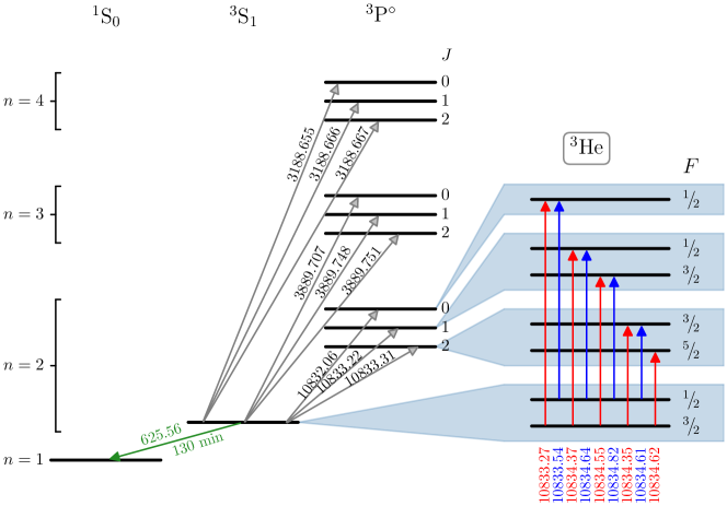
Figure 3: Grotrian diagram (not to scale) showing the energy levels of the lowest levels of the helium triplet state. All ⁴He i* transitions used in this work are shown in gray. The hyperfine structure of the $n=2$ level of ³He is shown in the blue shaded boxes. The blue and red arrows indicate transitions from the $F=0.5$ and $F=1.5$ levels, respectively. The decay of metastable helium to the singlet state is represented by a green arrow. All wavelengths are shown in units of Å.

The helium absorption lines analyzed in this paper originate from the metastable $2^{3}$S state of He i, which has a lifetime of $\sim 130~{}{\rm min}$. This state is populated by recombinations from the He ii state, when the recombining electron has the same spin as the electron in the He ii ground state. The excited-state of the absorption lines (the ${}^{3}{\rm P}^{\rm o}$ state) exhibits fine-structure, with total angular momentum quantum numbers $J^{\prime}=0,1,2$, while the ground state of metastable helium (the ${}^{3}{\rm S}$ state) has $J=1$.

We use the energy levels compiled by Morton et al. (2006) to determine the vacuum wavelengths of the helium transitions used in this paper. The oscillator strengths ($f$) for the ⁴He transitions were retrieved from the National Institutes of Standards and Technology (NIST) Atomic Spectral Database (ASD) (Kramida et al., 2020). These oscillator strengths were also used for the ³He transitions, however, because ³He has a nuclear spin $I=1/2$, each fine-structure level with $J>0$ is split into two levels with $F=J\pm 1/2$. In some cases, this hyperfine splitting is comparable to the fine-structure splitting, and may affect the shape of the line profile. To account for this, we calculate the relative probability of the transitions to the excited hyperfine levels as the product of the level degeneracies and the Wigner $6J$-symbol (see e.g. Murphy & Berengut 2014):

$$S=(2F+1)(2F^{\prime}+1)\begin{Bmatrix}J&F&I\\ F^{\prime}&J^{\prime}&1\end{Bmatrix}^{2}$$ (1)

Finally, the natural damping constant ($\gamma_{ul}$) of each transition was computed by summing the spontaneous transition probabilities ($A_{ul}$; retrieved from Kramida et al. 2020) to all lower levels,

$$\gamma_{ul}=\sum_{l}A_{ul}$$ (2)

All of the atomic data are compiled in Table 1, and a Grotrian diagram of the most relevant transitions is shown in Figure 3. We also list the ³He isotope shift of each transition in the final column of Table 1. Note that the isotope shift is largest for the He i* $\lambda 1.0833\,\mu$m line, with an $f$-weighted isotope shift of $\sim+36.6~{}{\rm km~{}s}^{-1}$. Also note that the typical isotope shift is different for the 2s$\rightarrow$2p, 2s$\rightarrow$3p, and 2s$\rightarrow$4p, transitions; by comparing the profiles of He i* $\lambda 3889$Å and He i* $\lambda 1.0833\,\mu$m, we can unambiguously determine if a He i* $\lambda 1.0833\,\mu$m absorption feature is due to ³He, or if it is due to coincident ⁴He absorption located at $\sim+36.6~{}{\rm km~{}s}^{-1}$ relative to the dominant absorption component (see Section 4.2).

Lastly, throughout this work we assume that the excitation fractions of ³He i* and ⁴He i* are identical, so that the intrinsic helium isotope ratio is simply ³He/⁴He = $N(^{3}$He i*)/$N(^{4}$He i*). Given the similar ionization potential of the helium isotopes, we expect charge transfer reactions between ³He and ⁴He to ensure this assumption is a reliable one. However, we note that this assumption may need to be considered in more detail when the precision of this measurement improves.

4 Analysis

Our new CRIRES data reveal that the strength and structure of the ⁴He i* $\lambda 1.0833\,\mu$m absorption profile is quiescent and qualitatively similar to the expected profile based on the optical data that have been acquired over the past $\sim 30$ years (O’dell et al., 1993; Cox et al., 2017). This suggests that He i* is approximately in ionization equilibrium, since the lifetime of the metastable state ($\sim 130~{}{\rm min}$) is significantly less than the time between the observations. Furthermore, at the expected location of the ³He i* absorption, we detect a significant absorption feature ($>13\sigma$) with a rest frame equivalent width of $EW=3.64\pm 0.22$ mÅ (see top right panel of Figure 4). Note, this $EW$ measure is a blend of the transitions to the $J^{\prime}=1,2$ levels, so the effective oscillator strength of this absorption feature is $f_{\rm 1,2}=0.4794$ (i.e. the sum of all $f$ values in Table 1 with an upper state 1s2p ${}^{3}{\rm P}^{\rm o}_{1}$ and 1s2p ${}^{3}{\rm P}^{\rm o}_{2}$). Given that this feature is extremely weak, we can estimate the corresponding ³He i* column density towards $\Theta^{2}$A Ori using the relation (Spitzer, 1978):

$$\log_{10}\,N(^{3}{\rm He\,\textsc{i}^{*}})/{\rm cm}^{-2} = 20.053+\log_{10}\bigg{(}\frac{EW}{\lambda_{0}^{2}\,f_{\rm 1,2}}\bigg{)}$$ (3)

$$= 9.863\pm 0.027$$

where $EW$ and $\lambda_{0}$ are in units of Å and $\lambda_{0}\simeq 10834.6$ Å is the approximate rest-frame wavelength of ³He. In the following subsection, we perform a detailed profile analysis to determine the ³He/⁴He ratio along the line-of-sight to $\Theta^{2}$A Ori.

4.1 Profile fitting

To model the He i* absorption lines, we use the Absorption LIne Software (alis) package. alis uses a Levenberg-Marquardt algorithm to determine the model parameters that best-fit the data, by minimizing the chi-squared statistic. We perform a simultaneous fit to the stellar continuum, the interstellar absorption, the wavelength calibration, the zero-level, telluric absorption, and the instrument resolution. This fitting approach allows us to propagate the uncertainties of these quantities to the model parameters.

Before describing the implementation of this fitting procedure in detail, we first draw attention to a faint emission feature that is detected in the red wing ($\sim+23~{}{\rm km~{}s}^{-1}$) of the He i*$\,\lambda 1.0833\,\mu$m profile (see Figure 1). While this emission is largely removed as part of the differencing process (see Section 2), we note that the absorbing medium may be relatively thin owing to the conditions required for He i* absorption. As a result, some He i* emission may be superimposed on the He i* absorption, and this may become particularly pronounced in the wings of the profile as the absorption becomes optically thin. We therefore model the zero-level of this line with two Gaussian profiles in addition to a constant offset. The centroids of these two Gaussians have a fixed separation of 1.216 Å, which corresponds to the wavelength difference between the $J^{\prime}=0$ and $J^{\prime}=1,2$ levels. We note that this choice does not impact the weak ³He i* absorption line profile (see Section 4.2).

We model the stellar continuum as a high order Legendre polynomial, and the instrument resolution is assumed to be well-described by a Gaussian profile. The wavelength calibration is assumed to be correct for the He i* $\lambda 3188$ Å line (since it is the weakest He i* line detected), and we include model parameters to apply a small shift and stretch correction to the wavelength scales of the He i* $\lambda 3889$ Å and $\lambda 1.0833\,\mu$m lines. We fit directly to the total column density of ⁴He i* and the column density ratio, $N(^{3}$He i*)/$N(^{4}$He i*). As described in Section 3, we assume that charge transfer reactions ensure that the intrinsic helium isotope ratio ³He/⁴He = $N(^{3}$He i*)/$N(^{4}$He i*).

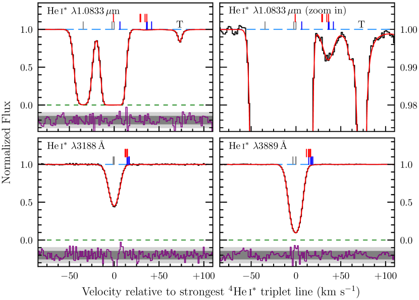
Figure 4: Spectra of a He i* absorption line system towards $\Theta^{2}$A Ori (top and bottom panels show the CRIRES and UVES data, respectively). The best-fitting model (red curves) are overlaid on the data (black histogram). The (data–model)/error residuals are shown at the bottom of each panel (purple histogram), while the 68 and 95 per cent confidence intervals are shown as the dark and light shaded bands, respectively. The corrected zero-level is shown by the green dashed line, while the normalized continuum is shown as the long-dashed blue line. Tick marks above each spectrum show the locations of the ⁴He i^∗ absorption (gray ticks) and the ³He i^∗ absorption (blue and red ticks indicate the $F=0.5$ and $F=1.5$ levels, respectively; cf. the same color scheme as in Figure 3). The top right panel is a zoom in of the top left panel. The feature marked with a T corresponds to two telluric absorption features, comprising a weak feature at $\sim+60~{}{\rm km~{}s}^{-1}$ and the main component at $\sim+70~{}{\rm km~{}s}^{-1}$. The reduced chi-squared of the best-fitting model is $\chi^{2}/{\rm dof}=1.104$.

Interstellar absorption lines are traditionally modelled with a Voigt profile, which assumes that the gas is distributed as a Maxwellian. Given the high S/N data involved, we noticed that the profile is asymmetric about the line centre, and is therefore not well-modelled by a single Voigt profile; a two component Voigt profile model is also insufficient to fully describe the line profile, within the uncertainties of our very high S/N data.

We have therefore modelled the line shape using a linear spline with a fixed knot spacing of $3-4~{}{\rm km~{}s}^{-1}$ (roughly corresponding to the instrument resolution). The linear spline is then convolved with a Gaussian profile (the width of this Gaussian is a free parameter) to construct a smooth and continuous, arbitrary line profile that is positive-definite. This process is therefore a hybrid between Voigt profile fitting and the apparent optical depth method (Savage & Sembach, 1991); we fit a smooth, arbitrary representation of the line profile shape, which is simultaneously represented by multiple absorption lines.

Our derivation follows a very similar procedure to that formulated by Savage & Sembach (1991). The observed line profile is given by the convolution of the intrinsic line profile, $I(\lambda)$, with the instrument profile, $\phi(\sigma_{\rm inst})$. The intrinsic line profile is given by:

$$I(\lambda)=I(\lambda)_{0}\,e^{-\tau(\lambda)}$$ (4)

where $I(\lambda)_{0}$ is the continuum and $\tau(\lambda)=N\,\sigma(\lambda)$ is the optical depth profile, which consists of the total column density ($N$) and the absorption cross section, $\sigma(\lambda)$. We can express the cross section in terms of the velocity relative to the center of the profile:

$$\sigma(v)=\frac{\pi\,e^{2}}{m_{\rm e}\,c^{2}}\,f\,\lambda_{0}\,c\,{\cal S}(v)$$ (5)

where $e^{2}/m_{\rm e}\,c^{2}$ is the classical electron radius, $\lambda_{0}$ is the rest wavelength of the transition, $f$ is the corresponding oscillator strength, $c$ is the speed of light, and ${\cal S}(v)$ is a smooth, normalized spline function, which is the convolution of a linear spline, ${\cal L}(v)$, with a Gaussian of velocity width $\sigma_{v}$:

$${\cal S}(v)={\cal L}(v)\,\circledast\,G(\sigma_{v}).$$ (6)

To summarise, the free parameters of this function include the column density ($N$), the Gaussian convolution width ($\sigma_{v}$), and the line shape values at each spline knot of the linear spline, ${\cal L}(v)$. Note that the redshift of the line is not a free parameter of the function; it is fixed at a value that is close to the maximum optical depth, since the redshift is degenerate with changing the line profile weights at each spline knot. The model profile is generated on a sub-pixel scale of $1.5~{}{\rm m~{}s}^{-1}$ (corresponding to a sub-pixellation factor of 1000) and rebinned to the native pixel resolution ($1.5~{}{\rm km~{}s}^{-1}$) after the model is convolved with the instrument profile.

We stress that it is the combined information of the shape and strength of the absorption features that allow us to pin down the column density; the shape of the line core is largely set by the weak ³He i* absorption, while the rest of the line shape is set by the stronger ⁴He i* absorption. The relative strength of the lines then sets the ³He/⁴He ratio. So, even though the cores of the ⁴He i* $\lambda 1.0833\,\mu$m line profiles appear saturated, the absorption lines are fully resolved and the S/N is very high; there is sufficient information about the profile shape from just the He i* $\lambda 1.0833\,\mu$m line profile to pin down the ⁴He i* column density and the ³He/⁴He ratio using all of the contributing absorption features that make up the complete line profile (i.e. the ⁴He i* transitions to the $J^{\prime}=0$ and $J^{\prime}=1,2$ levels, in combination with the ³He i* transitions to the $J^{\prime}=1,2$ levels). The higher order optical/UV transitions are also important to determine the ⁴He i* column density, because they are weaker and are situated in the linear regime of the curve of growth.

However, given that the optical and near-infrared data were taken $\sim 7$ years apart, the absorption profile might not be expected to have exactly the same shape at the two epochs, given the very high S/N of the data. We therefore model a separate spline to the UVES and CRIRES data, but all spline models are assumed have the same ³He/⁴He ratio. Finally, there are several telluric absorption lines that are located near the He i* $\lambda 1.0833\,\mu$m absorption line; we model these telluric features as a Voigt profile with an additional damping term to account for collisional broadening.

Finally, the relative population of the $F=0.5$ and $F=1.5$ hyperfine levels of ³He i* is given by:

$$\frac{n_{0.5}}{n_{1.5}}=\frac{g_{0.5}}{g_{1.5}}\exp(-T_{\star}/T_{s})$$ (7)

where $g_{0.5}=2$ and $g_{1.5}=4$ are the level degeneracies, $T_{\star}=0.32~{}{\rm K}$, and $T_{s}$ is the spin temperature. Given that the spin temperature is expected to greatly exceed $T_{\star}$, the relative population of the $F=0.5$ and $F=1.5$ hyperfine levels is simply given by the ratio of the level degeneracies; as part of the fitting procedure, we appropriately weight the ³He i* transitions to account for the relative populations of the ground state. The data and the best-fitting model are shown in Figure 4; the reduced chi-squared of this fit is $\chi^{2}/{\rm dof}=1.104$.

The best-fitting model corresponds to a total metastable ⁴He i* column density of $\log_{10\,}N(^{4}{\rm He\,\textsc{i}^{*}})/{\rm cm}^{-2}=13.6430\pm 0.0031$ based solely on the He i* $\lambda 1.0833\,\mu$m absorption in the CRIRES data. The optical data (based on a simultaneous fit to both He i* $\lambda 3188$ Å and $\lambda 3889$ Å) suggests a higher value of $\log_{10\,}N(^{4}{\rm He\,\textsc{i}^{*}})/{\rm cm}^{-2}=13.6972\pm 0.0023$, which is statistically inconsistent with the CRIRES data. This difference may reflect a real change to the line profile depth between the two epochs of observation, and highlights the importance of recording as many absorption lines simultaneously; the weak higher order transitions are optically thin, and can be used to pin down the column density of ⁴He i* more reliably. Given the current data, the column density of He i* is decreasing at a rate of $-(2.29\pm 0.16)\times 10^{9}~{}{\rm atoms~{}cm}^{-2}~{}{\rm yr}^{-1}$; at this rate, the He i* absorption will be short-lived ($\sim 20,000~{}{\rm years}$). This noticeable change between the two epochs could be due to the transverse motion of the cloud, or a reduction in the ionization parameter at the surface of the absorbing medium (Liu et al., 2015). Future optical data covering the weak He i* $\lambda 3188$ absorption will help to pin down the time evolution of the strength and line-of-sight motion of this profile. For the present analysis, we do not use the optical absorption lines to determine the helium isotope ratio.

As mentioned earlier, we perform a direct fit to the total helium isotope ratio. The best-fitting value of the absorbing gas cloud towards $\Theta^{2}$A Ori is:

$$\log_{10}~{}^{3}{\rm He}/^{4}{\rm He}=-3.752\pm 0.032$$ (8)

or expressed as a linear quantity:

$$^{3}{\rm He}/^{4}{\rm He}=(1.77\pm 0.13)\times 10^{-4}$$ (9)

This corresponds to a seven per cent determination of the helium isotope ratio, and is currently limited only by the S/N. As a sanity check of this measurement, we use the ³He i* column density estimated from the equivalent width of the ³He i* $\lambda 1.0833\,\mu$m absorption feature (Equation 3) in combination with the ⁴He i* column density based on the alis fits, to infer a helium isotope ratio of ³He/⁴He $=(1.66\pm 0.10)\times 10^{-4}$. This estimate is consistent with the value based on our alis fits (Equation 9); the difference between these two values of ³He/⁴He and their uncertainties, is due to the uncertain continuum placement when estimating the equivalent width (i.e. Equation 3 does not include the uncertainty due to continuum placement). This highlights the benefit of simultaneously fitting the continuum and the absorption lines with alis: The continuum uncertainty is folded into all parameter values, and avoids introducing a systematic bias due to the manual placement of the continuum.

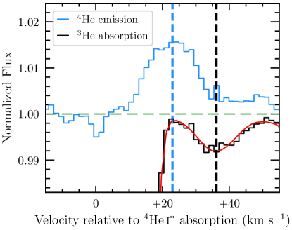
Figure 5: Spectrum of $\Theta^{2}$A Ori (black histogram) overlaid with the best-fitting model (red curve). The blue histogram shows the surrounding ⁴He i* emission that appears on the red wing of the absorption profile (cf. Figure 1); the emission profile has been offset by $+1$ (but is the same relative scale as the black histogram), to allow a close comparison to the absorption profile. The horizontal green dashed line simultaneously represents the normalized continuum of $\Theta^{2}$A Ori, and the zero-level of the ⁴He i* emission line. The vertical blue and black dashed lines indicate the centroids of the ⁴He i* emission and ³He i* absorption, respectively.

4.2 Validation

We performed several checks to validate the detection of ³He i* absorption towards $\Theta^{2}$A Ori. First, we confirmed that there are no telluric absorption lines that are coincident with the locations of either the ³He i* or the ⁴He i* absorption. The only telluric lines nearby are those identified in Figure 4.

As mentioned in Section 2, to optimize the final combined S/N, we subtracted two raw frames at different nod positions before extraction. We also extracted spectra of $\Theta^{2}$A Ori using the individual raw frames. The final combined S/N of the data based on this ‘alternative’ reduction is $\sim 600$ in the continuum, a factor of $\gtrsim 2$ lower than using differencing. Nevertheless, we confirmed that the ³He i* absorption feature is present in the alternative reduction, and is therefore not an artifact of the frame differencing.

We also note that the faint ⁴He i* emission seen in Figure 1 is not aligned with the ³He i* absorption feature (see Figure 5). Thus, the ³He i* absorption feature is not an artifact of subtracting frames at two different nod positions. Moreover, we note that the faint ⁴He i* emission feature peaks at $\sim+23~{}{\rm km~{}s}^{-1}$ relative to the absorption (or, $\sim+25~{}{\rm km~{}s}^{-1}$ in the heliocentric frame). The location and width of this emission feature is not easily attributable to any of the velocity structures previously identified in Orion (O’dell et al., 1993). Curiously, the peak of this emission feature is located at the point of minimum optical depth in the red wing of the ⁴He i* absorption feature. Thus, the emission feature may be caused by photons that are recombining at the face of the He i* absorbing medium. These photons escape from the cloud where the optical depth is lowest.

Finally, we consider the rare possibility that the ³He i* absorption feature is actually due to coincident ⁴He i* absorption that occurs at exactly the expected location and strength of the ³He i* absorption feature. In principle, this obscure possibility can be ruled out by searching for the corresponding ⁴He i* absorption in the optical/UV absorption lines, since the isotope shift is different for different transitions. We investigated this possibility for the UVES data currently available, but these data are not of high enough S/N to rule out the possibility of satellite ⁴He i* absorption. However, we note that the red wing of the He i* $\lambda 3889$ Å absorption feature is clean and featureless to the noise level of the current data, so the possibility of satellite ⁴He i* absorption can be ruled out with future data.

5 Results

³He has only been detected a handful of times, and never outside of the Milky Way; many of these detections come from observations or studies of Solar System objects, while the rest are based on observations of the ³He⁺ $8.7~{}{\rm GHz}$ line from H ii regions (Balser & Bania, 2018). In this section, we discuss how measurements of the helium isotope ratio can inform models of Galactic chemical enrichment and stellar nucleosynthesis. Observations of ³He/⁴He can also be used for cosmology and to study the physics of the early Universe.

5.1 Galactic Chemical Evolution of ³He

To interpret our new determination of the Galactic helium isotope ratio, we performed a series of galactic chemical evolution (GCE) models using the Versatile Integrator for Chemical Evolution (VICE; Johnson & Weinberg 2020). Our implementation closely follows the model described by Johnson et al. (2021); we briefly summarise the key aspects of this model below, and refer the reader to Johnson et al. (2021) for further details.

There are two key motivations for using VICE in this work. First, the combination of an inside-out star formation history and radial migration has already been shown to reproduce many chemical properties and the abundance structure of the Milky Way using these VICE models (Johnson et al., 2021). Thus, to ensure this agreement is maintained, the only changes that we make to the Johnson et al. (2021) model are the ³He and ⁴He yields, and the starting primordial composition. The second motivation for using VICE is its numerically-constrained model of radial migration which allows stellar populations to enrich distributions of radii as their orbits evolve. This is an important ingredient in GCE models of the Milky Way because stellar populations may move significant distances before nucleosynthetic events with long delay times occur; Johnson et al. (2021) discuss this effect at length for the production of iron by Type Ia supernovae. Since the dominant ³He yield comes from low mass stars with long lifetimes (e.g. Larson 1974, Maeder & Meynet 1989), it is possible that similar processes may affect the distribution of ³He in the Galaxy.

VICE models the Milky Way as a series of concentric rings of uniform width $\delta R_{\text{gal}}$ out to a radius of 20 kpc, and we retain the choice of $\delta R_{\text{gal}}=100$ pc from Johnson et al. (2021). The gas surface density of each ring is given by the gas mass in each ring, divided by the area of the ring, where the gas mass is determined by a balance of infall, outflow, star formation, and the gas returned from stars. Our models assume an inside-out star formation history (SFH), with a functional form:

$$\dot{\Sigma}_{\star}(t|R_{\rm gal})\propto(1-e^{-t/\tau_{\rm rise}})\,e^{-t/\tau_{\rm sfh}}$$ (10)

where $R_{\rm gal}$ represents the galactocentric radius at the center of each ring, $\tau_{\rm rise}=2~{}{\rm Gyr}$ (i.e. the star formation history peaks around a redshift $z\approx 2.5$), and $\tau_{\rm sfh}$ is the e-folding timescale of the star formation history, which depends on $R_{\rm gal}$. The relationship between $\tau_{\rm sfh}$ and $R_{\rm gal}$ is based on a fit to the relationship between stellar surface density and age of a sample of Sa/Sb spiral galaxies (Sánchez 2020; see Figure 3 of Johnson et al. 2021). We set the star formation rate to zero when $R_{\rm gal}>15.5~{}{\rm kpc}$. The star formation law we adopt is a piecewise power law with three intervals defined by the gas surface density; the intervals and power law indices are based on the aggregate observational data by Bigiel et al. (2010) and Leroy et al. (2013), in combination with the theoretically motivated star formation laws presented by Krumholz et al. (2018). Outflows are characterized by a mass-loading factor, $\eta=\dot{M}_{\rm out}/\dot{M}_{\star}$, where $\dot{M}_{\rm out}$ is the outflow rate, and $\dot{M}_{\star}$ is the star formation rate. The radial dependence of our outflow prescription ensures that the late-time abundance gradient of oxygen agrees with observations (Weinberg et al., 2017). We assume a Kroupa (2001) stellar initial mass function (IMF).

Our model implements a radial migration of stars from their birth radius based on the outputs from the h277 cosmological simulation (Christensen et al., 2012; Zolotov et al., 2012; Loebman et al., 2012, 2014; Brooks & Zolotov, 2014). The only quantities used from this simulation are the galactocentric birth radius, birth time, and the final galactocentric radius (the radius at the end of the simulation) of each star particle. We assume that stars make a smooth, continuous migration from their birth radius to their final radius with a displacement proportional to the square root of the star’s age. This functional form is similar to the assumption used by Frankel et al. (2020) to model the radial migration of stars due to angular momentum diffusion. We simulate our Milky Way models for 13.2 Gyr, which is set by the outputs of the h277 simulation; given the age of the Universe ($13.801\pm 0.024~{}{\rm Gyr}$; Planck Collaboration et al. 2020), star formation begins in our Milky Way models $\sim 0.6~{}{\rm Gyr}$ after the Big Bang ($z\approx 9$).

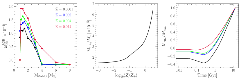
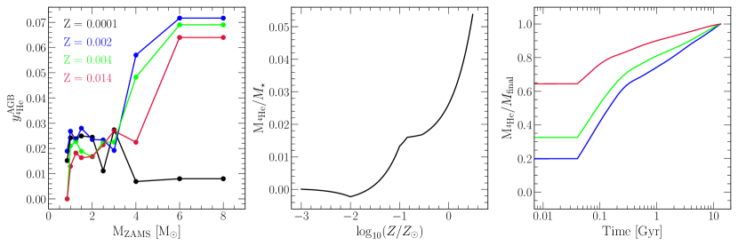
Figure 6: The ³He and ⁴He yields of AGB stars (top and bottom panels, respectively). Left panels: fractional yield as a function of the zero age main sequence (ZAMS) stellar mass. The yield of ³He is dominated by the lowest mass stars, while the yield of ⁴He is dominated by intermediate and high mass stars. Middle panels: IMF integrated yield as a function of metallicity for a simple stellar population, normalized by the total stellar mass. The yields of both ³He and ⁴He are greater for higher metallicity stellar populations. Right panels: fractional time evolution of ³He and ⁴He for a simple stellar population. The ³He yield is dominated by the lowest mass stars. As a result, radial migration is expected to be important for understanding the galactic chemical evolution of ³He/⁴He. We note that the $Z=0.0001$ curve is not shown in the bottom right panel for ⁴He, because extremely metal-poor massive stars net destroy more ⁴He than AGB stars net produce.

The key aspect of our models that differs from Johnson et al. (2021) is the choice of nucleosynthesis yields. Although VICE in its current version does not natively compute isotope-specific GCE models, the code base is built on a generic system of equations that make it easily extensible. For stars that undergo core-collapse ($M>8\,{\rm M}_{\odot}$), VICE instantaneously deposits an IMF-weighted yield at the birth annulus. We calculate the IMF-weighted ($M>8\,{\rm M}_{\odot}$) metallicity-dependent net yields of ⁴He and ³He using the nucleosynthesis calculations of Limongi & Chieffi (2018); we then linearly interpolate these IMF-weighted massive star yields over metallicity in VICE. For example, at $Z={\rm Z_{\odot}}$, for every solar mass of stars formed in a ring, $0.065~{}{\rm M_{\odot}}$ of ⁴He is immediately returned to the ISM in that ring, of which $0.017~{}{\rm M_{\odot}}$ is freshly synthesized and $r\,Y_{\rm ISM}=0.048~{}{\rm M_{\odot}}$ is recycled, where $Y_{\rm ISM}\simeq 0.255$ is the ISM ⁴He mass fraction and $r=0.19$ is the recycling fraction for $M>8~{}{\rm M_{\odot}}$ stars assuming a Kroupa (2001) IMF and that all stars with $M>8~{}{\rm M_{\odot}}$ form a $1.44~{}{\rm M}_{\odot}$ compact remnant. The corresponding amount of hydrogen returned to the ISM is $0.076~{}{\rm M_{\rm\odot}}$. The amount of ³He returned to the ISM is $5.9\times 10^{-6}~{}{\rm M_{\odot}}$, which is lower than the recycled fraction ($7.4\times 10^{-6}~{}{\rm M_{\odot}}$). Thus, the massive star yields that we employ act to reduce the ³He/⁴He ratio at solar metallicity. We note, however, that the ³He and ⁴He yields of massive stars play a relatively minor role in the chemical evolution of ³He/⁴He; ignoring the yields of massive stars would result in an increase of the present day ³He/⁴He of Orion by $\sim 4$ per cent.

For asymptotic giant branch (AGB) stars ($M<8\,{\rm M}_{\odot}$), we adopt the metallicity dependent net yields of ³He and ⁴He reported by Lagarde et al. (2011, 2012). Since the Lagarde et al. (2011, 2012) yields are only computed for $M\leq 6\,{\rm M}_{\odot}$, we assume that $8\,{\rm M}_{\odot}$ stars have the same net ⁴He yield as $6\,{\rm M}_{\odot}$ stars, while we assume the same ³He yield for $8\,{\rm M}_{\odot}$ stars for all metallicities ($y_{\rm{}^{3}He}^{\rm AGB}=-1.75\times 10^{-5}$). We then linearly interpolate these yields over metallicity and stellar mass. We assume the Larson (1974) metallicity-independent mass-lifetime relation for our calculations, and checked that our results were unchanged by using metallicity-dependent prescriptions (Hurley et al., 2000; Vincenzo et al., 2016). In Figure 6, we show the fractional ³He and ⁴He net yields as a function of stellar mass and metallicity (left panels), the IMF-weighted yield as a function of metallicity (middle panels), and the gradual build up of ³He and ⁴He for a simple stellar population (right panels). Taken together, these plots demonstrate that the lowest mass stars ($M\lesssim 2\,{\rm M}_{\odot}$) are chiefly responsible for the production of ³He, and this largely drives the evolution of the ³He/⁴He ratio. This is particularly true for solar metallicity AGB stars. As mentioned earlier in this Section, a key motivation of including the effects of radial migration is that the dominant ³He yield comes from stars with the longest lifetimes, and therefore most likely to deposit their yield far from their birth galactocentric radius.

We also update the primordial composition of VICE; using the Planck Collaboration et al. (2020) determination of the baryon density (100 $\Omega_{\rm B,0}\,h^{2}$ $=2.242\pm 0.014$), the latest value of the neutron lifetime ($\tau_{\rm n}=879.4\pm 0.6\,{\rm s}$; Particle Data Group et al. 2020), the $d(p,\gamma)^{3}{\rm He}$ rate reported by the Laboratory for Underground Nuclear Astrophysics (LUNA; Mossa et al. 2020), and assuming the Standard Model of particle physics and cosmology ($N_{\rm eff}=3.044$; Mangano et al. 2005; de Salas & Pastor 2016; Grohs & Fuller 2017; Akita & Yamaguchi 2020; Escudero Abenza 2020; Froustey et al. 2020; Bennett et al. 2020), we determine the primordial helium isotope ratio to be (³He/⁴He)${}_{\rm p}=(1.257\pm 0.017)\times 10^{-4}$ (see Pitrou et al. 2021; Yeh et al. 2021).

Before we use this model to infer the galactic chemical evolution of ³He/⁴He, it is worthwhile keeping in mind that some model ingredients are still missing. For example, the VICE Milky Way model has been shown to produce a broad range of [$\alpha$/Fe] at fixed [Fe/H] in the solar vicinity, but it does not produce a clear bimodality in [$\alpha$/Fe], in contrast with observations (Vincenzo et al., 2021). Johnson et al. (2021) conjecture that this discrepancy implies that the Milky Way’s accretion and/or star formation history is less continuous than the model assumes, and changing this history could also alter the evolution of ³He/⁴He. One mechanism that can help to produce a stronger [$\alpha$/Fe] bimodality is the two-infall scenario (Chiappini et al., 2001; Romano et al., 2010; Noguchi, 2018; Spitoni et al., 2019). While we do not consider alternative (e.g. two-infall or bursty) star formation history in this work, we note that the observed ³He/⁴He ratio near the Orion Nebula is just $\sim 40$ per cent above the Standard Model primordial value; galactic chemical evolution has apparently altered the ISM ratio only moderately relative to its primordial value, a conclusion supported by the apparent similarity of primordial and ISM D/H ratios (Linsky et al., 2006; Prodanović et al., 2010). Weinberg (2017) argues that this weak evolution of D/H is a consequence of substantial ongoing dilution of the ISM by infall, with much of the material processed through stars ejected in outflows (see also, Romano et al. 2006; Steigman et al. 2007). Similar considerations would apply to ³He/⁴He.

5.2 ³He in the Milky Way

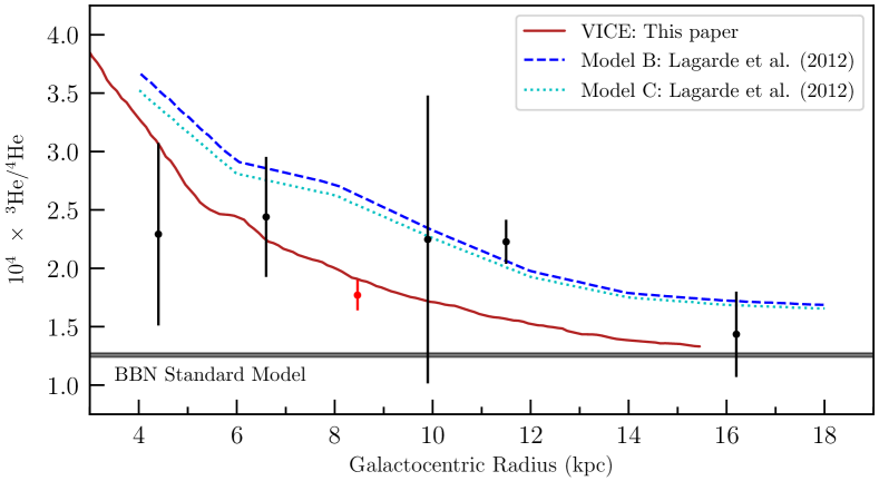
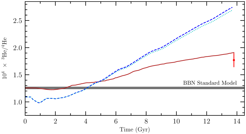
Figure 7: Present-day radial profile (top panel) and time evolution at the galactocentric radius of the Orion Nebula (bottom panel) of the helium isotope ratio. Our VICE galactic chemical enrichment model is shown as the red curve. This model assumes that all low mass stars undergo the thermohaline instability and rotational mixing. Model C uses the same low mass star yields, but different input physics (Lagarde et al., 2012). Model B assumes that 96 per cent of stars undergo the thermohaline instability and rotational mixing, while the yields of the remaining stars adopt the ‘standard’ stellar models (see Lagarde et al. 2012 for further details about model B and C, and see Section 5.1 for details about our VICE models). Note that the Lagarde et al. (2012) models assume a different primordial composition; for a fairer comparison, the Lagarde et al. (2012) models should be increased by about $0.15~{}\times 10^{-4}$. Our Orion Nebula ³He/⁴He determination is shown as the red symbol and error bar. In the top panel, we also overplot measures of the ³He/H abundance of Galactic H ii regions (Balser & Bania, 2018) converted to the helium isotope ratio using the estimated helium abundance of the H ii regions (see Equation 2 of Balser & Bania 2018). The primordial ³He/⁴He value, assuming the Standard Model, is shown by the horizontal dark gray bands, (³He/⁴He)${}_{\rm p}=(1.257\pm 0.017)\times 10^{-4}$.

Early models of stellar nucleosynthesis indicated that low mass ($1-3~{}{\rm M}_{\odot}$) stars yield copious amounts of ³He as part of the p-p chain while burning on the main sequence (Iben, 1967a, b; Rood, 1972). It was recognised soon after, in the context of GCE, that these stellar models may overpredict the amount of ³He compared to the protosolar value (Rood et al. 1976; see also, Truran & Cameron 1971). The stellar and GCE models were also at odds with the first observations of ³He from H ii regions (Rood et al., 1979). It was later recognized that the best determination of the ³He/H abundance came from observations of structurally simple H ii regions (Balser et al., 1999a; Bania et al., 2002). This pioneering work demonstrated that the ³He abundance of the Milky Way is mostly the same at different locations. Moreover, the value derived by Bania et al. (2002) is of similar magnitude to the protosolar value, indicating that the ³He abundance did not change significantly during the past 4.5 Gyr of Galactic evolution.

It became clear that models of stellar nucleosynthesis were overproducing ³He, and missing a critical ingredient, leading to the so-called ³He problem. Sackmann & Boothroyd (1999) proposed that additional mixing can help destroy ³He, and can alleviate the discrepancy between the protosolar ³He value and GCE models (Palla et al., 2000; Chiappini et al., 2002). A possible mechanism for the additional mixing — the thermohaline instability — was identified by Charbonnel & Zahn (2007a) as a physical mechanism to resolve the ³He problem (see also, Charbonnel & Zahn 2007b). Models of GCE combined with a grid of stellar models that employ the thermohaline instability and rotational mixing (Lagarde et al., 2011, 2012) were found to produce remarkable agreement with the protosolar and present day abundance of ³He in the Milky Way, as well as the radial profile of ³He from H ii regions (Balser & Bania, 2018).

In Figure 7, we show the present day radial ³He/⁴He profile (top panel) and the time evolution of ³He/⁴He at the galactocentric distance of the Orion Nebula (bottom panel). The red curve shows the results of our VICE models (see Section 5.1), and the red symbol and error bar represents our determination of the ³He/⁴He ratio of the Orion Nebula. We also overplot the results of two GCE models presented by Lagarde et al. (2012): Model B (blue dashed curve) assumes that 4 per cent of low mass stars obey the ‘standard’ stellar evolution models, while the remaining 96 per cent undergo the thermohaline instability and rotational mixing. Model C (cyan dotted curve) assumes that all low mass stars undergo the thermohaline instability and rotational mixing. Note, the initial primordial composition assumed by Lagarde et al. (2012) is lower than the current Standard Model value; correcting for this offset would result in Model B and C being shifted to higher ³He/⁴He values. The black symbols with error bars illustrate the latest ³He/H measures from (Balser & Bania, 2018), converted to a helium isotope ratio using the conversion (see their Equation 2):

$${}^{4}{\rm He/H}=0.105-1.75\times 10^{-3}~{}R_{\rm gal}.$$ (11)

The primordial helium isotope ratio, (³He/⁴He)${}_{\rm p}=(1.257\pm 0.017)\times 10^{-4}$, is shown by the horizontal dark gray bands in Figure 7. Our VICE models are in good agreement with our determination of the Orion helium isotope ratio and measures of the ³He/H abundance of Galactic H ii regions. The Lagarde et al. (2012) chemical evolution models are vertically offset from our VICE GCE models and does not provide as good fit to our determination of the Orion helium isotope ratio.

To diagnose this offset, we explored the sensitivity of various model parameters to the chemical evolution of ³He/⁴He. The conclusion of these tests is that the relative importance of outflows and inflows has the strongest impact on the chemical evolution of ³He/⁴He. With strong outflows, significant infall of primordial gas is necessary to sustain ongoing star formation, and a larger portion of the ISM is made up of unprocessed material. Models that have weaker outflows retain more freshly synthesized ³He in the ISM, leading to a higher ³He/⁴He ratio. The strength of outflows is currently an uncertain parameter in GCE models. Our VICE models employ strong outflows in order to reproduce the observed Milky Way oxygen gradient given our assumed IMF averaged yield of oxygen $y_{O}=0.015$ ($1.5M_{\odot}$ of oxygen produced per $100M_{\odot}$ of star formation). Some other GCE models omit outflows entirely (e.g., Spitoni et al. 2019, 2021), and can still produce an acceptable disc if this oxygen yield is much lower, perhaps because of a steeper IMF or more extensive black hole formation (Griffith et al., 2021). Like (D/H), the ³He/⁴He ratio may offer important constraints on the strength of outflows because much of the ISM ³He and ⁴He are primordial in origin and thus sourced by ongoing accretion (see Section 5.3 below). As a side note, we found that the stellar IMF and the mass-lifetime relation of stars have a negligible impact on our results.

5.3 Implications for Cosmology

Since our determination of the helium isotope ratio is obtained from a relatively metal-enriched environment, the composition that we measure does not directly reflect the primordial ³He/⁴He ratio. However, we consider two approaches below that allow us to infer the most likely primordial ³He/⁴He ratio, based on the currently available data: An empirical measure, and a model-dependent determination.

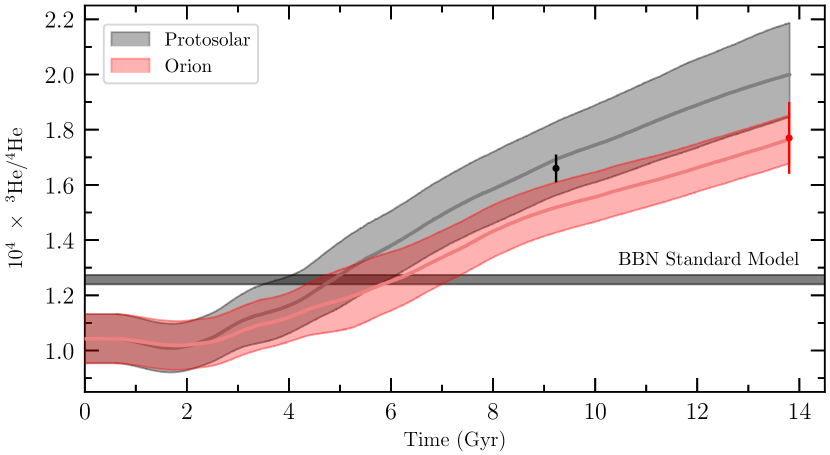
Figure 8: The time evolution of the Milky Way ³He/⁴He ratio according to our VICE Galactic Chemical Evolution models (gray and red bands). The gray band is for a galactocentric radius of $7.3\pm 0.6\,{\rm kpc}$ (corresponding to the birth galactocentric radius of the Sun), while the red band is for $8.47\,{\rm kpc}$ (corresponding to the galactocentric radius of Orion). The black and red symbols with error bars are the protosolar measurement and present day Orion measurement of ³He/⁴He, respectively. The width of each band represents the $1\sigma$ uncertainty of the primordial ³He/⁴He ratio. Note that the width of the gray band also includes the uncertainty of the birth galactocentric radius of the Sun. The horizontal dark gray band represents the Standard Model value of the primordial ³He/⁴He ratio.

We first consider an empirical assessment of the primordial ³He/H ratio, based on a similar approach as that outlined by Yang et al. (1984). We start by converting our measure of the helium isotope ratio to a ³He abundance, using the measured ⁴He/H ratio of the Orion nebula (${\rm{}^{4}He/H}=0.0913\pm 0.0042$; Mesa-Delgado et al. 2012); we estimate that the ³He abundance of Orion is ${}^{3}{\rm He/H}=(1.62\pm 0.14)\times 10^{-5}$. We then note the following inequality:

$$\bigg{(}\frac{{}^{3}{\rm He+D}}{\rm H}\bigg{)}_{\rm p}\leq\bigg{(}\frac{{}^{3}{\rm He+D}}{\rm H}\bigg{)}_{\dagger}$$ (12)

where subscript ‘p’ refers to the primordial value, and the subscript ‘$\dagger$’ refers to the Orion value. This inequality holds because: (1) Essentially all D is burnt into ³He at temperatures $\gtrsim 6\times 10^{5}~{}{\rm K}$; and (2) Models of stellar nucleosynthesis indicate that the dominant ³He yield comes from low mass stars, which are net producers of ³He. Rearranging this inequality, we can solve for the primordial ³He/H ratio, given the measured values of the primordial deuterium abundance $({\rm D/H})_{\rm p}=(2.527\pm 0.030)\times 10^{-5}$ (Cooke et al., 2018), and the interstellar deuterium abundance ${\rm(D/H)}_{\dagger}=(2.0\pm 0.1)\times 10^{-5}$ (Prodanović et al., 2010). Combined with our estimate of the Orion ³He/H ratio, we find:

$$(^{3}{\rm He/H})_{\rm p}\leq(1.09\pm 0.18)\times 10^{-5}$$ (13)

where the uncertainties of the interstellar helium and deuterium abundances contribute almost equally to the total quoted uncertainty. This limit is in agreement with the Standard Model value, $(^{3}{\rm He/H})_{\rm p}=(1.039\pm 0.014)\times 10^{-5}$ (Pitrou et al., 2021; Yeh et al., 2021).

In addition to our empirical limit on the primordial ³He abundance, we also consider a model-dependent estimate of the primordial helium isotope ratio, based on our best available understanding of stellar nucleosynthesis and chemical evolution. We use our VICE GCE models to infer the best-fitting primordial ³He/⁴He, given two time-separated determinations of the helium isotope ratio of the Milky Way: The first measure is the protosolar value, which is based on a measurement of Jupiter’s atmosphere by the Galileo Probe Mass Spectrometer (Mahaffy et al., 1998) (i.e. a snapshot of the Milky Way helium isotope ratio some $4.5~{}{\rm Gyr}$ ago). The second determination that we use is the present day Milky Way value reported in this paper. These two values are remarkably comparable, and are only slightly elevated above the Standard Model value. Given the very gradual change to the primordial ⁴He/H abundance over time ($\sim 11$ per cent), this suggests that the build up of ³He, even in a galaxy such as the Milky Way, is relatively gradual, probably because infall continually drives it back toward the primordial value. Thus, even in a chemically evolved galaxy, such as the Milky Way, we can still estimate the primordial ³He/⁴He ratio because: (1) The build up of ³He is gradual over time; and (2) We have two time-separated measures of the ³He/⁴He ratio covering one-third of the Milky Way’s age.

GCE models indicate that the ³He/⁴He value depends on both galactocentric radius and the amount of time that has passed since the start of chemical evolution. The present day measurement of the ³He/⁴He ratio towards $\Theta^{2}$A Ori is based on a gas cloud in the vicinity of the Orion Nebula, estimated to be at a galactocentric radius of $\sim 8.5\,{\rm kpc}$. The current age of the Universe is $13.801\pm 0.024\,{\rm Gyr}$ (Planck Collaboration et al., 2020), which in our case corresponds to the final output of the VICE models. The protosolar ³He/⁴He measurement reflects the Milky Way value at the birth of the Solar System $4.5682\,{\rm Gyr}$ ago (Bouvier & Wadhwa, 2010). The birth galactocentric radius of the Sun is estimated to be somewhat closer to the galactic center than the present distance, due to a combination of radial heating and angular momentum diffusion (Minchev et al., 2018; Frankel et al., 2020); in our analysis, we use the semi-empirical result of Minchev et al. (2018, $R_{\rm gal,\odot}=7.3\pm 0.6\,{\rm kpc}$).

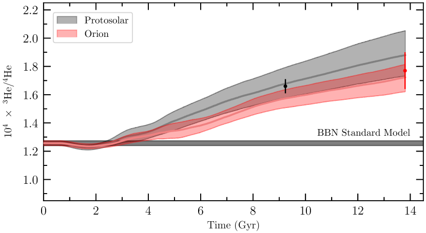
Figure 9: Same as Figure 8, but the VICE model shown here assumes the Standard Model ³He/⁴He ratio and allows the strength of the outflow prescription to vary as a free parameter. The best-fit models scale the default outflow mass loading efficiencies upward by a factor $f_{s}=1.7$.

We generated a suite of VICE models covering a grid of primordial ³He/⁴He values. For each ³He/⁴He value, we take an average of 16 VICE simulations to minimize the post-BBN scatter of ³He/⁴He values due to radial migration (this scatter is of order $1-2$ per cent). We include this scatter as part of the model uncertainty, even though this is subdominant compared to the measurement errors. To determine the most likely value of the primordial ³He/⁴He ratio, we linearly interpolated over our averaged grid of VICE models, and then conducted a Markov Chain Monte Carlo analysis using the emcee software (Foreman-Mackey et al., 2013). We assume a uniform prior on the ³He/⁴He ratio, and a Gaussian prior on the birth galactocentric radius of the Sun, as described above. We note that, aside from the assumptions stated above, the only free parameter of this model is the primordial ³He/⁴He value. Given our VICE model, the best-fit value and 68 per cent confidence interval of the primordial ³He/⁴He ratio is:

$$(^{3}{\rm He}/^{4}{\rm He})_{\rm p}=(1.043\pm 0.089)\times 10^{-4}$$ (14)

We remind the reader that this value is model dependent, and the error term does not include the (presently unknown) uncertainty associated with the nucleosynthetic yields and the GCE model. However, given that this determination is within $2.4\sigma$ of the Standard Model value, (³He/⁴He)${}_{\rm p}=(1.257\pm 0.017)\times 10^{-4}$ without accounting for the unknown model error, we consider our result to be in agreement with the Standard Model to within $\sim 2\sigma$. Given that our model has a single free parameter — the primordial ³He/⁴He ratio — it is remarkable that our GCE model and yields can simultaneously reproduce the protosolar and present day values of the Galactic ³He/⁴He ratio without any tuning. The time evolution of our best-fit model is shown in Figure 8, where the gray and red shaded regions are for the protosolar and present day ³He/⁴He, respectively.

We also consider an alternative model where we fix the primordial ³He/⁴He to the Standard Model value, and tune the strength of the outflow prescription to match the currently available data. The relative contributions of outflows (removing freshly synthesised ³He and ⁴He) and inflows (of primordial material) is the dominant factor that sets the GCE of ³He/⁴He. In our model the gas surface density is determined by the star formation rate and the empirically motivated star formation law (Johnson et al., 2021), so a higher outflow also implies a higher inflow to replenish the gas supply. For our alternative model, we scale the strength of our outflow prescription uniformly at all radii, so that $\eta_{\rm new}=f_{s}\,\eta$. As described in Section 5.1, the radial dependence and strength of the outflow prescription is defined in VICE to match the late-time abundance gradient of oxygen to observations (Weinberg et al., 2017). Thus, by rescaling the strength of outflows with the above prescription, we are altering the abundance distribution of oxygen in our models. In order to reconcile these rescaled models with the late-time abundance gradient of oxygen, the total oxygen yield would need to be comparably scaled (i.e. stronger outflows require a higher oxygen yield to match the data).

We generated a grid of VICE models where the outflows are uniformly scaled by $f_{s}$, and sampled this grid using an MCMC analysis similar to that described earlier. We determine a best-fitting value of the outflow scale factor, $f_{s}=1.70_{-0.25}^{+0.31}$, which is able to simultaneously reproduce the protosolar and present-day value of the ³He/⁴He ratio, assuming the Standard Model primordial ³He/⁴He value. The time evolution of the ³He/⁴He ratio of the Milky Way for this alternative model is shown in Figure 9. Our models presume that gas ejected in outflows has the same chemical composition as the ambient ISM. We have not examined models where the winds are preferentially composed of massive star ejecta, which might arise if core collapse supernovae are the primary wind drivers, but we expect that they would require higher outflow mass-loading because more of the ³He produced by low mass stars would be retained. Finally, we note that the combination of D/H and ³He/⁴He may provide strong constraints on the strength of outflows and thus indirectly constrain the scale of the yields, since: (1) both D and ³He are primordial, and for the Standard Model, D/H and ³He/⁴He are known; (2) D is completely burnt into ³He; and (3) ³He is net produced by low mass stars.

5.4 Future prospects

Helium-3 is rarely detected in any environment, and never outside of the Milky Way. The new approach developed in this paper offers a precise measure of the helium isotope ratio, and is currently limited only by the S/N of the observations. Future measurements along different sightlines toward the Orion Nebula may further improve this determination, and test the consistency of this technique. Several sightlines suitable for carrying out this test are already known towards the brightest stars in Orion (O’dell et al., 1993; Oudmaijer et al., 1997). Going further, He i* absorption is also detected towards $\zeta$ Oph (Galazutdinov & Krelowski, 2012) and several stars in the cluster NGC 6611 (Evans et al., 2005) in the Milky Way, that would permit a measure of the radial ³He/⁴He abundance gradient (see Figure 7) and obtain further tests of our GCE model and pin down the inferred primordial abundance.

Another critical goal is to measure ³He/⁴He in more metal-poor environments. Fortuitously, the Small and Large Magellanic Clouds offer the perfect laboratory for carrying out such an exploration. Suitable stars in the Magellanic Clouds are bright enough ($m_{\rm J}\simeq 12-15$) to confidently detect ($5\sigma$) a ³He i* absorption line with an equivalent width, $EW=3.6~{}{\rm m\AA}$ (i.e. identical to the feature towards $\Theta^{2}$A Ori) in $\sim 50$ hours with the upgraded VLT+CRIRES. This exposure time could be reduced for sightlines with a higher He i* column density. While challenging, this experiment is achievable with current facilities if suitable targets can be identified.

Finally, we note that it may be possible to detect ³He in absorption against gamma-ray burst or quasar spectra; strong He i* absorption has already been detected towards GRB 140506A at redshift $z=0.889$ (Fynbo et al., 2014), but to reach the requisite S/N, a detection of ³He i* may require a significant investment of telescope time and rapid response observations. Because GRBs fade on short timescales ($\lesssim 1~{}{\rm day}$), this may only be possible with the next generation of $30+$ m telescopes.

6 Conclusions

We have presented the first detection of metastable ³He i* absorption using the recently upgraded CRIRES spectrograph at the VLT, as part of science verification. The absorption, which occurs along the line-of-sight to $\Theta^{2}$A Ori in the Orion Nebula, is detected at high confidence ($>13\sigma$), and has allowed us to directly measure the helium isotope ratio for the first time beyond the Local Interstellar Cloud. Our conclusions are summarized as follows:

(i) The helium isotope ratio in the vicinity of the Orion Nebula is found to be ${}^{3}{\rm He}/^{4}{\rm He}=(1.77\pm 0.13)\times 10^{-4}$, which is roughly $\sim 40$ per cent higher than the primordial abundance assuming the Standard Model of particle physics and cosmology.

(ii) We calculated a suite of galactic chemical evolution models with VICE using the best available chemical yields of low mass stars that undergo the thermohaline instability and rotational mixing. This model confirms previous calculations that the ³He/⁴He ratio decreases with increasing galactocentric radius. Our model, which reproduces many chemical properties and the abundance structure of the Milky Way, is in good agreement with our measurement of ³He/⁴He.

(iii) We use these models to perform a joint fit to the present day (Orion Nebula) ³He/⁴He value and the protosolar value (a snapshot of the Milky Way $\sim 4.5~{}{\rm Gyr}$ ago), allowing only the primordial helium isotope ratio to vary. Our models can reproduce both time-separated measurements if the primordial helium isotope ratio is $(^{3}{\rm He}/^{4}{\rm He})_{\rm p}=(1.043\pm 0.089)\times 10^{-4}$, which agrees with the Standard Model value to within $\sim 2\sigma$. We remind the reader that the quoted confidence interval does not include the model and yield uncertainty. We also report a more conservative, empirical limit on the primordial ³He abundance $(^{3}{\rm He/H})_{\rm p}\leq(1.09\pm 0.18)\times 10^{-5}$, which is based on the measured ⁴He/H ratio of Orion, and the amount of primordial deuterium that has been burnt into ³He.

(iv) As an alternative to this analysis, we can reproduce the protosolar and present-day values of ³He/⁴He if we assume the Standard Model primordial ³He/⁴He value and scale the strength of outflows in our VICE models. However, the strength of the outflows would need to be uniformly increased by a scaling factor $f_{s}=1.70_{-0.25}^{+0.31}$, which would in turn require comparable increase in oxygen and iron yields to retain the empirical successes of this model found by Johnson et al. (2021). Our measured ³He/⁴He ratio offers a stringent test for Milky Way chemical evolution models.

Detecting ³He i* absorption is challenging due to the rarity of metastable helium absorbers, and the high S/N required to secure a confident detection of a weak absorption feature. Although the Milky Way is not the ideal environment to secure an estimate of the primordial abundance, future measurements of ³He/⁴He in the Milky Way will allow us to better understand the galactic chemical evolution of ³He. Furthermore, if suitable sightlines can be found towards stars in nearby star-forming dwarf galaxies, or along the line-of-sight to a low redshift gamma-ray burst (e.g. Fynbo et al. 2014), this approach may offer a reliable technique to pin down the primordial helium isotope ratio, and thereby test the Standard Model of particle physics and cosmology in a new way. However, such an ambitious goal may have to wait until the forthcoming generation of telescopes with $30+\,{\rm m}$ aperture. Observations of local dwarf galaxies will require a high contrast between the stellar and nebula emission, to ensure that the surrounding He i* emission does not contribute significantly to the noise in the vicinity of the weak ³He i* absorption line. Observations of gamma-ray bursts will require that the GRB: (1) explodes in a metal-poor environment; (2) is at sufficiently low redshift ($z\lesssim 0.66$) so that the He i* $\lambda 1.0833\,\mu$m absorption line can still be detected with future facilities (Marconi et al., 2021); and (3) is sufficiently bright for a long enough time that the required S/N can be achieved.

Finally, we point out that three primordial abundance measurements — D/H, ⁴He/H, and ³He/⁴He — all agree with the Standard Model values to within $\sim 20$ per cent or much better. This is in stark contrast to the observationally inferred primordial ⁷Li/H abundance, which disagrees with the Standard Model value by $\sim 350$ per cent (see the review by Fields 2011). It is therefore becoming increasingly difficult to explain this discrepancy — dubbed the Cosmic Lithium Problem — with physics beyond the Standard Model, without breaking the remarkable simultaneous agreement of the primordial D/H, ⁴He/H and ³He/⁴He ratios with the Standard Model of particle physics and cosmology.

References

- Akita & Yamaguchi (2020) Akita, K., & Yamaguchi, M. 2020, J. Cosmology Astropart. Phys, 2020, 012, doi: 10.1088/1475-7516/2020/08/012
- Aoki et al. (2009) Aoki, W., Barklem, P. S., Beers, T. C., et al. 2009, ApJ, 698, 1803, doi: 10.1088/0004-637X/698/2/1803
- Asplund et al. (2006) Asplund, M., Lambert, D. L., Nissen, P. E., Primas, F., & Smith, V. V. 2006, ApJ, 644, 229, doi: 10.1086/503538
- Astropy Collaboration et al. (2013) Astropy Collaboration, Robitaille, T. P., Tollerud, E. J., et al. 2013, A&A, 558, A33, doi: 10.1051/0004-6361/201322068
- Astropy Collaboration et al. (2018) Astropy Collaboration, Price-Whelan, A. M., Sipőcz, B. M., et al. 2018, AJ, 156, 123, doi: 10.3847/1538-3881/aabc4f
- Aver et al. (2021) Aver, E., Berg, D. A., Olive, K. A., et al. 2021, J. Cosmology Astropart. Phys, 2021, 027, doi: 10.1088/1475-7516/2021/03/027
- Balser & Bania (2018) Balser, D. S., & Bania, T. M. 2018, AJ, 156, 280, doi: 10.3847/1538-3881/aaeb2b
- Balser et al. (1999a) Balser, D. S., Bania, T. M., Rood, R. T., & Wilson, T. L. 1999a, ApJ, 510, 759, doi: 10.1086/306598
- Balser et al. (2006) Balser, D. S., Goss, W. M., Bania, T. M., & Rood, R. T. 2006, ApJ, 640, 360, doi: 10.1086/499937
- Balser et al. (1999b) Balser, D. S., Rood, R. T., & Bania, T. M. 1999b, ApJ, 522, L73, doi: 10.1086/312216
- Bania & Balser (2021) Bania, T. M., & Balser, D. S. 2021, ApJ, 910, 73, doi: 10.3847/1538-4357/abd543
- Bania et al. (2002) Bania, T. M., Rood, R. T., & Balser, D. S. 2002, Nature, 415, 54, doi: 10.1038/415054a
- Bennett et al. (2020) Bennett, J. J., Buldgen, G., de Salas, P. F., et al. 2020, arXiv e-prints, arXiv:2012.02726. https://arxiv.org/abs/2012.02726
- Bigiel et al. (2010) Bigiel, F., Leroy, A., Walter, F., et al. 2010, AJ, 140, 1194, doi: 10.1088/0004-6256/140/5/1194
- Bouvier & Wadhwa (2010) Bouvier, A., & Wadhwa, M. 2010, Nature Geoscience, 3, 637, doi: 10.1038/ngeo941
- Brooks & Zolotov (2014) Brooks, A. M., & Zolotov, A. 2014, ApJ, 786, 87, doi: 10.1088/0004-637X/786/2/87
- Busemann et al. (2000) Busemann, H., Baur, H., & Wieler, R. 2000, \maps, 35, 949, doi: 10.1111/j.1945-5100.2000.tb01485.x
- Busemann et al. (2006) Busemann, H., Bühler, F., Grimberg, A., et al. 2006, ApJ, 639, 246, doi: 10.1086/499223
- Charbonnel & Zahn (2007a) Charbonnel, C., & Zahn, J. P. 2007a, A&A, 467, L15, doi: 10.1051/0004-6361:20077274
- Charbonnel & Zahn (2007b) —. 2007b, A&A, 476, L29, doi: 10.1051/0004-6361:20078740
- Chiappini et al. (2001) Chiappini, C., Matteucci, F., & Romano, D. 2001, ApJ, 554, 1044, doi: 10.1086/321427
- Chiappini et al. (2002) Chiappini, C., Renda, A., & Matteucci, F. 2002, A&A, 395, 789, doi: 10.1051/0004-6361:20021314
- Christensen et al. (2012) Christensen, C., Quinn, T., Governato, F., et al. 2012, MNRAS, 425, 3058, doi: 10.1111/j.1365-2966.2012.21628.x
- Cooke (2015) Cooke, R. J. 2015, ApJ, 812, L12, doi: 10.1088/2041-8205/812/1/L12
- Cooke & Fumagalli (2018) Cooke, R. J., & Fumagalli, M. 2018, Nature Astronomy, 2, 957, doi: 10.1038/s41550-018-0584-z
- Cooke et al. (2014) Cooke, R. J., Pettini, M., Jorgenson, R. A., Murphy, M. T., & Steidel, C. C. 2014, ApJ, 781, 31, doi: 10.1088/0004-637X/781/1/31
- Cooke et al. (2018) Cooke, R. J., Pettini, M., & Steidel, C. C. 2018, ApJ, 855, 102, doi: 10.3847/1538-4357/aaab53
- Cox et al. (2017) Cox, N. L. J., Cami, J., Farhang, A., et al. 2017, A&A, 606, A76, doi: 10.1051/0004-6361/201730912
- Cyburt et al. (2016) Cyburt, R. H., Fields, B. D., Olive, K. A., & Yeh, T.-H. 2016, Reviews of Modern Physics, 88, 015004, doi: 10.1103/RevModPhys.88.015004
- De Cia et al. (2021) De Cia, A., Jenkins, E. B., Fox, A. J., et al. 2021, Nature, 597, 206, doi: 10.1038/s41586-021-03780-0
- de Salas & Pastor (2016) de Salas, P. F., & Pastor, S. 2016, J. Cosmology Astropart. Phys, 2016, 051, doi: 10.1088/1475-7516/2016/07/051
- Dorn et al. (2014) Dorn, R. J., Anglada-Escude, G., Baade, D., et al. 2014, The Messenger, 156, 7
- Escudero Abenza (2020) Escudero Abenza, M. 2020, J. Cosmology Astropart. Phys, 2020, 048, doi: 10.1088/1475-7516/2020/05/048
- Evans et al. (2005) Evans, C. J., Smartt, S. J., Lee, J. K., et al. 2005, A&A, 437, 467, doi: 10.1051/0004-6361:20042446
- Fernández et al. (2019) Fernández, V., Terlevich, E., Díaz, A. I., & Terlevich, R. 2019, MNRAS, 487, 3221, doi: 10.1093/mnras/stz1433
- Fields (2011) Fields, B. D. 2011, Annual Review of Nuclear and Particle Science, 61, 47, doi: 10.1146/annurev-nucl-102010-130445
- Fields et al. (2020) Fields, B. D., Olive, K. A., Yeh, T.-H., & Young, C. 2020, J. Cosmology Astropart. Phys, 2020, 010, doi: 10.1088/1475-7516/2020/03/010
- Foreman-Mackey et al. (2013) Foreman-Mackey, D., Hogg, D. W., Lang, D., & Goodman, J. 2013, PASP, 125, 306, doi: 10.1086/670067
- Frankel et al. (2020) Frankel, N., Sanders, J., Ting, Y.-S., & Rix, H.-W. 2020, ApJ, 896, 15, doi: 10.3847/1538-4357/ab910c
- Froustey et al. (2020) Froustey, J., Pitrou, C., & Volpe, M. C. 2020, J. Cosmology Astropart. Phys, 2020, 015, doi: 10.1088/1475-7516/2020/12/015
- Fynbo et al. (2014) Fynbo, J. P. U., Krühler, T., Leighly, K., et al. 2014, A&A, 572, A12, doi: 10.1051/0004-6361/201424726
- Galazutdinov & Krelowski (2012) Galazutdinov, G. A., & Krelowski, J. 2012, MNRAS, 422, 3457, doi: 10.1111/j.1365-2966.2012.20856.x
- Griffith et al. (2021) Griffith, E. J., Sukhbold, T., Weinberg, D. H., et al. 2021, ApJ, 921, 73, doi: 10.3847/1538-4357/ac1bac
- Grohs & Fuller (2017) Grohs, E., & Fuller, G. M. 2017, Nuclear Physics B, 923, 222, doi: 10.1016/j.nuclphysb.2017.07.019
- Guzman-Ramirez et al. (2016) Guzman-Ramirez, L., Rizzo, J. R., Zijlstra, A. A., et al. 2016, MNRAS, 460, L35, doi: 10.1093/mnrasl/slw070
- Harris et al. (2020) Harris, C. R., Millman, K. J., van der Walt, S. J., et al. 2020, Nature, 585, 357, doi: 10.1038/s41586-020-2649-2
- Heber et al. (2012) Heber, V. S., Baur, H., Bochsler, P., et al. 2012, ApJ, 759, 121, doi: 10.1088/0004-637X/759/2/121
- Hsyu et al. (2020) Hsyu, T., Cooke, R. J., Prochaska, J. X., & Bolte, M. 2020, ApJ, 896, 77, doi: 10.3847/1538-4357/ab91af
- Hunter (2007) Hunter, J. D. 2007, Computing in Science & Engineering, 9, 90, doi: 10.1109/MCSE.2007.55
- Hurley et al. (2000) Hurley, J. R., Pols, O. R., & Tout, C. A. 2000, MNRAS, 315, 543, doi: 10.1046/j.1365-8711.2000.03426.x
- Iben (1967a) Iben, Icko, J. 1967a, ApJ, 147, 624, doi: 10.1086/149040
- Iben (1967b) —. 1967b, ApJ, 147, 650, doi: 10.1086/149041
- Izotov et al. (2014) Izotov, Y. I., Thuan, T. X., & Guseva, N. G. 2014, MNRAS, 445, 778, doi: 10.1093/mnras/stu1771
- Johnson & Weinberg (2020) Johnson, J. W., & Weinberg, D. H. 2020, MNRAS, 498, 1364, doi: 10.1093/mnras/staa2431
- Johnson et al. (2021) Johnson, J. W., Weinberg, D. H., Vincenzo, F., et al. 2021, MNRAS, 508, 4484, doi: 10.1093/mnras/stab2718
- Kaeufl et al. (2004) Kaeufl, H.-U., Ballester, P., Biereichel, P., et al. 2004, in Society of Photo-Optical Instrumentation Engineers (SPIE) Conference Series, Vol. 5492, Ground-based Instrumentation for Astronomy, ed. A. F. M. Moorwood & M. Iye, 1218–1227, doi: 10.1117/12.551480
- Khullar et al. (2020) Khullar, S., Ma, Q., Busch, P., et al. 2020, MNRAS, 497, 572, doi: 10.1093/mnras/staa1951
- Korn et al. (2006) Korn, A. J., Grundahl, F., Richard, O., et al. 2006, Nature, 442, 657, doi: 10.1038/nature05011
- Kramida et al. (2020) Kramida, A., Yu. Ralchenko, Reader, J., & and NIST ASD Team. 2020, NIST Atomic Spectra Database (ver. 5.8), [Online]. Available: https://physics.nist.gov/asd [2017, April 9]. National Institute of Standards and Technology, Gaithersburg, MD.
- Krietsch et al. (2021) Krietsch, D., Busemann, H., Riebe, M. E. I., et al. 2021, Geochim. Cosmochim. Acta, 310, 240, doi: 10.1016/j.gca.2021.05.050
- Kroupa (2001) Kroupa, P. 2001, MNRAS, 322, 231, doi: 10.1046/j.1365-8711.2001.04022.x
- Krumholz et al. (2018) Krumholz, M. R., Burkhart, B., Forbes, J. C., & Crocker, R. M. 2018, MNRAS, 477, 2716, doi: 10.1093/mnras/sty852
- Kurichin et al. (2022) Kurichin, O. A., Kislitsyn, P. A., & Ivanchik, A. V. 2022, arXiv e-prints, arXiv:2201.06431. https://arxiv.org/abs/2201.06431
- Lagarde et al. (2011) Lagarde, N., Charbonnel, C., Decressin, T., & Hagelberg, J. 2011, A&A, 536, A28, doi: 10.1051/0004-6361/201117739
- Lagarde et al. (2012) Lagarde, N., Romano, D., Charbonnel, C., et al. 2012, A&A, 542, A62, doi: 10.1051/0004-6361/201219132
- Larson (1974) Larson, R. B. 1974, MNRAS, 166, 585, doi: 10.1093/mnras/166.3.585
- Leroy et al. (2013) Leroy, A. K., Walter, F., Sandstrom, K., et al. 2013, AJ, 146, 19, doi: 10.1088/0004-6256/146/2/19
- Limongi & Chieffi (2018) Limongi, M., & Chieffi, A. 2018, ApJS, 237, 13, doi: 10.3847/1538-4365/aacb24
- Lind et al. (2009) Lind, K., Primas, F., Charbonnel, C., Grundahl, F., & Asplund, M. 2009, A&A, 503, 545, doi: 10.1051/0004-6361/200912524
- Linsky et al. (2006) Linsky, J. L., Draine, B. T., Moos, H. W., et al. 2006, ApJ, 647, 1106, doi: 10.1086/505556
- Liu et al. (2015) Liu, W.-J., Zhou, H., Ji, T., et al. 2015, ApJS, 217, 11, doi: 10.1088/0067-0049/217/1/11
- Loebman et al. (2012) Loebman, S. R., Ivezić, Ž., Quinn, T. R., et al. 2012, ApJ, 758, L23, doi: 10.1088/2041-8205/758/1/L23
- Loebman et al. (2014) —. 2014, ApJ, 794, 151, doi: 10.1088/0004-637X/794/2/151
- Maeder & Meynet (1989) Maeder, A., & Meynet, G. 1989, A&A, 210, 155
- Mahaffy et al. (1998) Mahaffy, P. R., Donahue, T. M., Atreya, S. K., Owen, T. C., & Niemann, H. B. 1998, Space Sci. Rev., 84, 251
- Mangano et al. (2005) Mangano, G., Miele, G., Pastor, S., et al. 2005, Nuclear Physics B, 729, 221, doi: 10.1016/j.nuclphysb.2005.09.041
- Marconi et al. (2021) Marconi, A., Abreu, M., Adibekyan, V., et al. 2021, The Messenger, 182, 27, doi: 10.18727/0722-6691/5219
- Matas Pinto et al. (2021) Matas Pinto, A., Spite, M., Caffau, E., et al. 2021, arXiv e-prints, arXiv:2110.00243. https://arxiv.org/abs/2110.00243
- McQuinn & Switzer (2009) McQuinn, M., & Switzer, E. R. 2009, Phys. Rev. D, 80, 063010, doi: 10.1103/PhysRevD.80.063010
- Meléndez et al. (2010) Meléndez, J., Casagrande, L., Ramírez, I., Asplund, M., & Schuster, W. J. 2010, A&A, 515, L3, doi: 10.1051/0004-6361/200913047
- Mesa-Delgado et al. (2012) Mesa-Delgado, A., Núñez-Díaz, M., Esteban, C., et al. 2012, MNRAS, 426, 614, doi: 10.1111/j.1365-2966.2012.21230.x
- Meurer et al. (2017) Meurer, A., Smith, C. P., Paprocki, M., et al. 2017, PeerJ Computer Science, 3, e103, doi: 10.7717/peerj-cs.103
- Minchev et al. (2018) Minchev, I., Anders, F., Recio-Blanco, A., et al. 2018, MNRAS, 481, 1645, doi: 10.1093/mnras/sty2033
- Morton et al. (2006) Morton, D. C., Wu, Q. X., & Drake, G. W. F. 2006, Canadian Journal of Physics, 84, 83, doi: 10.1139/P06-009
- Mossa et al. (2020) Mossa, V., Stöckel, K., Cavanna, F., et al. 2020, Nature, 587, 210, doi: 10.1038/s41586-020-2878-4
- Murphy & Berengut (2014) Murphy, M. T., & Berengut, J. C. 2014, MNRAS, 438, 388, doi: 10.1093/mnras/stt2204
- Noguchi (2018) Noguchi, M. 2018, Nature, 559, 585, doi: 10.1038/s41586-018-0329-2
- O’dell et al. (1993) O’dell, C. R., Valk, J. H., Wen, Z., & Meyer, D. M. 1993, ApJ, 403, 678, doi: 10.1086/172238
- Oudmaijer et al. (1997) Oudmaijer, R. D., Drew, J. E., Barlow, M. J., Crawford, I. A., & Proga, D. 1997, MNRAS, 291, 110, doi: 10.1093/mnras/291.1.110
- Palla et al. (2000) Palla, F., Bachiller, R., Stanghellini, L., Tosi, M., & Galli, D. 2000, A&A, 355, 69. https://arxiv.org/abs/astro-ph/9912086
- Particle Data Group et al. (2020) Particle Data Group, Zyla, P. A., Barnett, R. M., et al. 2020, Progress of Theoretical and Experimental Physics, 2020, doi: 10.1093/ptep/ptaa104
- Péron et al. (2018) Péron, S., Moreira, M., & Agranier, A. 2018, Geochemistry, Geophysics, Geosystems, 19, 979, doi: 10.1002/2017GC007388
- Pitrou et al. (2018) Pitrou, C., Coc, A., Uzan, J.-P., & Vangioni, E. 2018, Phys. Rep., 754, 1, doi: 10.1016/j.physrep.2018.04.005
- Pitrou et al. (2021) —. 2021, MNRAS, 502, 2474, doi: 10.1093/mnras/stab135
- Planck Collaboration et al. (2020) Planck Collaboration, Aghanim, N., Akrami, Y., et al. 2020, A&A, 641, A6, doi: 10.1051/0004-6361/201833910
- Prochaska et al. (2020) Prochaska, J., Hennawi, J., Westfall, K., et al. 2020, The Journal of Open Source Software, 5, 2308, doi: 10.21105/joss.02308
- Prodanović et al. (2010) Prodanović, T., Steigman, G., & Fields, B. D. 2010, MNRAS, 406, 1108, doi: 10.1111/j.1365-2966.2010.16734.x
- Romano et al. (2010) Romano, D., Karakas, A. I., Tosi, M., & Matteucci, F. 2010, A&A, 522, A32, doi: 10.1051/0004-6361/201014483
- Romano et al. (2006) Romano, D., Tosi, M., Chiappini, C., & Matteucci, F. 2006, MNRAS, 369, 295, doi: 10.1111/j.1365-2966.2006.10287.x
- Rood (1972) Rood, R. T. 1972, ApJ, 177, 681, doi: 10.1086/151747
- Rood et al. (1976) Rood, R. T., Steigman, G., & Tinsley, B. M. 1976, ApJ, 207, L57, doi: 10.1086/182178
- Rood et al. (1979) Rood, R. T., Wilson, T. L., & Steigman, G. 1979, ApJ, 227, L97, doi: 10.1086/182875
- Sackmann & Boothroyd (1999) Sackmann, I. J., & Boothroyd, A. I. 1999, ApJ, 510, 217, doi: 10.1086/306545
- Sánchez (2020) Sánchez, S. F. 2020, ARA&A, 58, 99, doi: 10.1146/annurev-astro-012120-013326
- Savage & Sembach (1991) Savage, B. D., & Sembach, K. R. 1991, ApJ, 379, 245, doi: 10.1086/170498
- Sbordone et al. (2010) Sbordone, L., Bonifacio, P., Caffau, E., et al. 2010, A&A, 522, A26, doi: 10.1051/0004-6361/200913282
- Seifahrt et al. (2010) Seifahrt, A., Käufl, H. U., Zängl, G., et al. 2010, A&A, 524, A11, doi: 10.1051/0004-6361/200913782
- Spitoni et al. (2019) Spitoni, E., Silva Aguirre, V., Matteucci, F., Calura, F., & Grisoni, V. 2019, A&A, 623, A60, doi: 10.1051/0004-6361/201834188
- Spitoni et al. (2021) Spitoni, E., Verma, K., Silva Aguirre, V., et al. 2021, A&A, 647, A73, doi: 10.1051/0004-6361/202039864
- Spitzer (1978) Spitzer, L. 1978, Physical processes in the interstellar medium, doi: 10.1002/9783527617722
- Steigman et al. (2007) Steigman, G., Romano, D., & Tosi, M. 2007, MNRAS, 378, 576, doi: 10.1111/j.1365-2966.2007.11780.x
- Takeuchi et al. (2014) Takeuchi, Y., Zaroubi, S., & Sugiyama, N. 2014, MNRAS, 444, 2236, doi: 10.1093/mnras/stu1550
- Truran & Cameron (1971) Truran, J. W., & Cameron, A. G. W. 1971, Ap&SS, 14, 179, doi: 10.1007/BF00649203
- Valerdi et al. (2021) Valerdi, M., Peimbert, A., & Peimbert, M. 2021, MNRAS, 505, 3624, doi: 10.1093/mnras/stab1543
- Vasiliev et al. (2019) Vasiliev, E. O., Sethi, S. K., & Shchekinov, Y. A. 2019, MNRAS, 490, 5057, doi: 10.1093/mnras/stz2964
- Vincenzo et al. (2016) Vincenzo, F., Matteucci, F., de Boer, T. J. L., Cignoni, M., & Tosi, M. 2016, MNRAS, 460, 2238, doi: 10.1093/mnras/stw1145
- Vincenzo et al. (2021) Vincenzo, F., Weinberg, D. H., Miglio, A., Lane, R. R., & Roman-Lopes, A. 2021, MNRAS, 508, 5903, doi: 10.1093/mnras/stab2899
- Virtanen et al. (2020) Virtanen, P., Gommers, R., Oliphant, T. E., et al. 2020, Nature Methods, 17, 261, doi: 10.1038/s41592-019-0686-2
- Weinberg (2017) Weinberg, D. H. 2017, ApJ, 851, 25, doi: 10.3847/1538-4357/aa96b2
- Weinberg et al. (2017) Weinberg, D. H., Andrews, B. H., & Freudenburg, J. 2017, ApJ, 837, 183, doi: 10.3847/1538-4357/837/2/183
- Wilson (1937) Wilson, O. C. 1937, PASP, 49, 338, doi: 10.1086/124868
- Yang et al. (1984) Yang, J., Turner, M. S., Steigman, G., Schramm, D. N., & Olive, K. A. 1984, ApJ, 281, 493, doi: 10.1086/162123
- Yeh et al. (2021) Yeh, T.-H., Olive, K. A., & Fields, B. D. 2021, J. Cosmology Astropart. Phys, 2021, 046, doi: 10.1088/1475-7516/2021/03/046
- Zolotov et al. (2012) Zolotov, A., Brooks, A. M., Willman, B., et al. 2012, ApJ, 761, 71, doi: 10.1088/0004-637X/761/1/71