Topological Expansion of Oscillatory BGW and HCIZ Integrals at Strong Coupling

1. Introduction

1.1. Overview

The purpose of this paper is to prove a longstanding conjecture on the asymptotic behavior of two particularly significant matrix integrals: the Bars-Green/Brézin-Gross-Witten/Wadia integral,

(1.1) $$I_{N}^{(1)}=\int_{\mathrm{U}(N)}e^{\sqrt{z}N\mathrm{Tr}(AU+BU^{-1})}\mathrm{d}U,$$

and the Harish-Chandra/Itzykson-Zuber integral,

(1.2) $$I_{N}^{(2)}=\int_{\mathrm{U}(N)}e^{zN\mathrm{Tr}AUBU^{-1}}\mathrm{d}U.$$

These are integrals over unitary matrices against unit mass Haar measure which depend on a complex parameter $z$ and a pair of complex matrices $A$ and $B$. The BGW and HCIZ integrals arise in many contexts throughout mathematics and physics, ranging from representation theory and random matrix theory to quantum field theory and statistical mechanics, and the following conjecture on their $N\to\infty$ asymptotics is widely known; see [23, 24, 52, 60, 62] and further references below.

Conjecture 1.1 (Topological Expansion Conjecture).

There exists a positive constant $\varepsilon$ such that, for each nonnegative integer $k$, we have

$$F_{N}=\sum_{g=0}^{k}N^{2-2g}F_{Ng}+o(N^{2-2k})$$

as $N\to\infty$, where $F_{N}=\log I_{N}$ and the error term is uniform over complex numbers $z$ of modulus at most $\varepsilon$ and complex matrices $A,B$ of spectral radius at most $1,$ with $F_{Ng}$ analytic functions of $z$ and the eigenvalues of $A$ and $B$ whose modulus is uniformly bounded in $N$. Moreover, $F_{Ng}$ is a generating function for combinatorial invariants of compact connected genus $g$ Riemann surfaces.

In stating Conjecture 1.1 we have introduced the following notational convention used throughout the paper: any declarative sentence in which the symbol $I_{N}$ appears without a superscript holds true for both (1.1) and (1.2). The same convention is applied to functions of these integrals, e.g. $F_{N}=\log I_{N}$. The superscript is restored whenever necessary or helpful.

The main result of this paper is a proof of Conjecture 1.1 — we show that the claimed logarithmic asymptotics of the oscillatory integrals $I_{N}^{(m)}$ do indeed exist, and enumerate branched covers of the Riemann sphere with at most $m$ non-simple branch points. The precise statement is Theorem 1.2 below.

The resolution of Conjecture 1.1 presented here has many potential applications. In particular, it should help clear the way for the development of Fourier-analytic techniques in the asymptotic spectral analysis of random matrices, and the parallel development of methods in asymptotic representation theory and integrable probability based on the orbit method. Moreover, the $m=1$ case should be useful for certain calculations in $\mathrm{U}(N)$ lattice gauge theory, while the $m=2$ case should have applications to multimatrix models in random matrix theory.

1.2. Background

The integrals (1.1) and (1.2) are analytic continuations of natural integral transforms: the former was studied by James [70] as the Fourier transform of Haar measure on $\mathrm{U}(N)$, while the latter was introduced by Harish-Chandra [65] as the Fourier transform of Haar measure on a given coadjoint orbit of $\mathrm{U}(N)$. Both are Bessel functions of matrix argument, a class of special functions introduced by Herz [66] whose properties at fixed rank $N$ have been studied from a variety of perspectives [27, 40, 57, 82].

The $N\to\infty$ asymptotic behavior of the integrals $I_{N}$ was first studied by theoretical physicists working in quantum field theory, and it was in this context that the first versions of Conjecture 1.1 emerged [6, 7, 15, 59, 69, 103, 109]. In particular, the hypothetical form of the asymptotic expansions claimed in Conjecture 1.1, as well as well as their supposed relation to Riemann surfaces, derives from the interplay between two fundamental approximation schemes used in quantum field theory — the strong coupling expansion [111] and the large $N$ expansion [1].

To explain further, let us view $I_{N}$ as the partition function of a Gibbs measure on $\mathrm{U}(N)$, with the complex variable $z$ playing the role of an inverse coupling/temperature parameter, and the complex matrices $A$ and $B$ being viewed as external fields. We shall see below that $I_{N}^{(2)}$ depends on $A$ and $B$ only through their eigenvalues $a_{1},\dots,a_{N},b_{1},\dots,b_{N}\in\mathbb{C}$, while $I_{N}^{(1)}$ depends on $A$ and $B$ only through the eigenvalues of their product, so that we may take $B$ to be the identity matrix in (1.1). Thus $I_{N}^{(m)}$ may be viewed as an entire function of $mN+1$ complex variables whose restriction to $\mathbb{R}^{mN+1}$ takes positive values, defining a true partition function in the sense of statistical physics. See [79] for some recent algorithmic results on sampling from the corresponding Gibbs measure in the case $m=2$.

Since $I_{N}=1$ at infinite coupling $z=0$, the free energy $F_{N}=\log I_{N}$ is defined and holomorphic in a neighborhood of the infinite coupling hyperplane $\{z=0\}\subset\mathbb{C}^{mN+1}$. Take the closed origin-centered polydisc $\mathbf{D}_{N}$ of unit polyradius $(1,\dots,1)$ in the phase space $\mathbb{C}^{mN}$ of the external field eigenvalues, embed it in the infinite coupling hyperplane, and thicken it out to $\mathbf{D}_{N}(\varepsilon)$, the closed origin-centered polydisc of polyradius $(\varepsilon,1,\dots,1)$ in $\mathbb{C}^{mN+1}$, i.e. the complex variables version of a compact box of height $2\varepsilon$ in the inverse coupling dimension and width $2$ in each of the $mN$ eigenvalue dimensions. By construction, $F_{N}$ vanishes on the null set $\mathbf{D}_{N}(0)\subset\mathbb{C}^{mN+1}$, and Conjecture 1.1 posits an approximation of this holomorphic function on the full-dimensional compact set $\mathbf{D}_{N}(\varepsilon)$ in the regime where $N\to\infty$ with $\varepsilon>0$ fixed.

The first claim made by Conjecture 1.1 is that this asymptotic problem is well-posed, in the sense that the thickening parameter $\varepsilon$ in the above construction may be selected irrespective of the dimension parameter $N$. It is not at all clear that this is the case, since a priori we know nothing about the geometry of the zeros of the partition function: for any given $\varepsilon>0$, it may be that the hypersurface $\{I_{N}=0\}$ and the polydisc $\mathbf{D}_{N}(\varepsilon)$ intersect nontrivially in $\mathbb{C}^{mN+1}$ for infinitely many $N\in\mathbb{N}$. For example, it is known [52, 107, 113] that the zero locus of $I_{N}^{(2)}$ in $\mathbb{C}^{2N+1}$ intersects $\mathbf{D}_{N}(\pi)=\mathbf{D}_{N}(3.14159265\dots)$ for all $N>1$, a fact which invalidates several spurious claims in the physics literature [56, 73]. Conjecture 1.1 is thus predicated on the existence of an absolute constant $\delta>0$ guaranteeing nonvanishing of $I_{N}$ on $\mathbf{D}_{N}(\delta)$, for all $N\in\mathbb{N}$. We shall refer to the hypothetical existence of such a constant $\delta$ as the stable non-vanishing hypothesis.

Assuming the stable non-vanishing hypothesis holds, the free energy $F_{N}$ belongs to the Banach algebra $(\mathcal{O}_{N}(\delta),\|\cdot\|_{\delta})$ of germs of holomorphic functions on $\mathbf{D}_{N}(\delta)$ equipped with sup norm, for all $N\in\mathbb{N}$. A natural way to approximate $F_{N}$ is then via its Maclaurin series, which converges $\|\cdot\|_{\delta}$-absolutely. The strong coupling expansion of $F_{N}$ is simply its Maclaurin series, written in the form

(1.3) $$F_{N}=\sum_{d=1}^{\infty}\frac{z^{d}}{d!}F_{N}^{d},$$

with the coefficients $F_{N}^{d}$ being viewed as homogeneous degree $d$ polynomial functions of the external field eigenvalues (the superscript $d$ is an index, not an exponent).

According to a fundamental principle in quantum field theory which lifts the apparatus of Feynman diagrams to matrix integrals [1, 12, 16, 69], and beyond [44, 76], the strong coupling coefficients $F_{N}^{d}$ are expected to stratify topologically as $N\to\infty$,

(1.4) $$F_{N}^{d}\sim\sum_{g=0}^{\infty}N^{2-2g}F_{Ng}^{d}.$$

The approximation (1.4) is a particular instance of a general ansatz in quantum field theory and statistical physics known variously as the large $N$ expansion, the $1/N$ expansion, the genus expansion, the topological expansion, or the ’t Hooft expansion; the leading term is called the planar limit, the spherical limit, or the ’t Hooft limit. The compendium [17] contains many fascinating examples of this device in action. In some situations, such as $\mathrm{U}(N)$ gauge theory [1] and Hermitian matrix models [16], the series (1.4) is actually a finite sum. This is not so in the the case at hand, which is associated with $\mathrm{U}(N)$ gauge theory on a lattice — in this case the expansion (1.4) is always infinite and almost always divergent [35].

The precise meaning of the expansion (1.4) in the present situation is that, for any fixed $d\in\mathbb{N}$ and fixed $k\in\mathbb{N}_{0},$ we should have

(1.5) $$\lim_{N\to\infty}N^{2k-2}\left\|F_{N}^{d}-\sum_{g=0}^{k}N^{2-2g}F_{Ng}^{d}\right\|=0,$$

where $\|\cdot\|$ is sup norm on bounded functions on the unit polydisc $\mathbf{D}_{N}\subset\mathbb{C}^{mN}$, and $F_{Ng}^{d}$ is a homogeneous degree $d$ polynomial in $mN$ variables which satisfies

(1.6) $$\sup_{N\in\mathbb{N}}\|F_{Ng}^{d}\|<\infty.$$

The topological feature of the polynomials $F_{Ng}^{d}$ alluded to above is that, when expressed as polynomials in the moments of the empirical eigenvalue distributions of the external fields, their coefficients are expected to be topological invariants of compact connected genus $g$ Riemann surfaces. Whereas the topological invariants underlying the large $N$ expansion in continuum gauge theory and Hermitian matrix models have long been known to be counts of isotopy classes of embedded graphs, a fact which has had many ramifications in mathematical physics [36, 112] and algebraic geometry [80], the topological invariants which presumably underly the large $N$ expansion in nonabelian lattice gauge theories have remained mysterious. It has even been argued that the leading order $F_{N0}^{d}$ in (1.4) does not consist of purely genus zero information [110]. See [95] for further discussion of these issues.

We will see below that the large $N$ expansion (1.4) of $F_{N}^{d}$ does indeed exist and that its coefficients $F_{Ng}^{d}$ admit a topological interpretation in terms of degree $d$ branched covers of the Riemann sphere by a compact connected genus $g$ surface, with at most $m$ non-simple branch points. We will also see that the series (1.4) converges uniformly absolutely on compact subsets of $\mathbb{C}^{mN}$ for $d\leq N$ (the stable range) but not for $d>N$ (the unstable range). Conjecture 1.1 expresses the hope that one can nevertheless plug the large $N$ expansion (1.4) into the strong coupling expansion (1.3),

(1.7) $$F_{N}=\sum_{d=1}^{\infty}\frac{z^{d}}{d!}F_{N}^{d}\longrightarrow\sum_{d=1}^{\infty}\frac{z^{d}}{d!}\sum_{g=0}^{\infty}N^{2-2g}F_{Ng}^{d},$$

change order of summation,

(1.8) $$\sum_{d=1}^{\infty}\frac{z^{d}}{d!}\sum_{g=0}^{\infty}N^{2-2g}F_{Ng}^{d}\longrightarrow\sum_{g=0}^{\infty}N^{2-2g}\sum_{d=1}^{\infty}\frac{z^{d}}{d!}F_{Ng}^{d},$$

and thereby arrive at an $N\to\infty$ asymptotic expansion of the free energy itself,

(1.9) $$F_{N}\sim\sum_{g=0}^{\infty}N^{2-2g}F_{Ng},$$

the coefficients of which are genus-specific generating functions,

(1.10) $$F_{Ng}=\sum_{d=1}^{\infty}\frac{z^{d}}{d!}F_{Ng}^{d}.$$

Conjecture 1.1 is thus claiming the existence of three absolute constants: a $\delta>0$ such that the integral $I_{N}$ is non-vanishing on $\mathbf{D}_{N}(\delta)$ for all $N$, a $\gamma>0$ such that the series $F_{Ng}$ converges uniformly absolutely on $\mathbf{D}_{N}(\gamma)$ for all $N$ and $g$, and finally an $\varepsilon\in(0,\delta)\cap(0,\gamma)$, such that

(1.11) $$\lim_{N\to\infty}N^{2k-2}\left\|F_{N}-\sum_{g=0}^{k}N^{2-2g}F_{Ng}\right\|_{\varepsilon}=0$$

holds for any fixed $k$.

The exchangeability of the large $N$ expansion and the strong coupling expansion has never been verified, and historically has been viewed with suspicion [59]. Instead, asymptotic studies of $F_{N}=\log I_{N}$ have proceeded along different lines, employing variational calculus [86], large deviation theory [63], asymptotics of Toeplitz determinants [71], and Schwinger-Dyson “loop” equations [15, 24, 62]. These approaches all have a common shortcoming: they only work when $I_{N}$ is restricted to the real domain $\mathbb{R}^{mN+1}\subset\mathbb{C}^{mN+1}$, so that oscillatory behavior of $I_{N}$ is suppressed and probabilistic estimates can be used. The restriction to real parameters is a substantial drawback, since as mentioned above the BGW and HCIZ integrals are natural Fourier kernels for Haar unitary random matrices and unitarily invariant Hermitian random matrices, respectively, which forces the issue of understanding their large $N$ behavior for complex coupling and complex external fields. While Fourier methods in random matrix theory and integrable probability are in active development [10, 19, 26, 45, 77, 85, 114], a persistent obstacle has been that only non-oscillatory asymptotics for the fundamental kernels (1.1) and (1.2) have so far been available.

1.3. Result

The main result of this paper is a proof of Conjecture 1.1. Throughout, $(\mathcal{O}_{N}(\rho),\|\cdot\|_{\rho})$ denotes the Banach algebra of germs of holomorphic functions on the closed origin-centered polydisc of polyradius $(\rho,1,\dots,1)$ in $\mathbb{C}^{mN+1}$, equipped with uniform norm. The unadorned norm $\|\cdot\|$ always means sup norm on bounded functions on the closed unit polydisc $\mathbf{D}_{N}$ in eigenvalue phase space $\mathbb{C}^{mN}$. Given a Young diagram $\alpha$, we write $\alpha\vdash d$ to indicate that $\alpha$ consists of $d$ cells. For a diagram $\alpha$ with $\ell(\alpha)$ rows and $\alpha_{i}$ cells in the $i$th row, let

(1.12) $$p_{\alpha}(x_{1},\dots,x_{N})=\prod_{i=1}^{\ell(\alpha)}\sum_{j=1}^{N}x_{j}^{\alpha_{i}}$$

denote the corresponding Newton symmetric polynomial in $N$ variables. Our main result is the following.

Theorem 1.2.

There exists $\varepsilon\in(0,\frac{2}{27})$ such that $I_{N}$ is nonvanishing on $\mathbf{D}_{N}(\varepsilon)$ for all $N\in\mathbb{N}$. Letting $F_{N}=\log I_{N}\in\mathcal{O}_{N}(\varepsilon)$, for each $k\in\mathbb{N}_{0}$ we have

$$\lim_{N\to\infty}N^{2k-2}\bigg{\|}F_{N}-\sum_{g=0}^{k}N^{2-2g}F_{Ng}\bigg{\|}_{\varepsilon}=0,$$

where

$$\begin{split}F_{Ng}^{(1)}&=\sum_{d=1}^{\infty}\frac{z^{d}}{d!}\sum_{\alpha\vdash d}\frac{p_{\alpha}(a_{1},\dots,a_{N})}{N^{\ell(\alpha)}}(-1)^{\ell(\alpha)+d}\vec{H}_{g}(\alpha),\\ F_{Ng}^{(2)}&=\sum_{d=1}^{\infty}\frac{z^{d}}{d!}\sum_{\alpha,\beta\vdash d}\frac{p_{\alpha}(a_{1},\dots,a_{N})}{N^{\ell(\alpha)}}\frac{p_{\beta}(b_{1},\dots,b_{N})}{N^{\ell(\beta)}}(-1)^{\ell(\alpha)+\ell(\beta)}\vec{H}_{g}(\alpha,\beta),\end{split}$$

and the positive integers $\vec{H}_{g}(\alpha)$, $\vec{H}_{g}(\alpha,\beta)$ are, respectively, the connected monotone single and double Hurwitz numbers of degree $d$ and genus $g$.

Monotone Hurwitz numbers, introduced in [50, 51] and further studied in many papers since, are combinatorial variants of the classical Hurwitz numbers familiar from enumerative geometry as counts of branched covers of the Riemann sphere with specified ramification data. The enumerative study of branched covers was initiated by Hurwitz in the 19th century [67, 68], and is now known as Hurwitz theory. Hurwitz theory remains relevant in contemporary enumerative geometry, being deeply intertwined with more sophisticated approaches to the enumeration of maps from curves to curves [97]. Hurwitz theory is the subject of a huge literature; see [42] for a quick introduction, [21] for a pedagogical treatment, [78] for a survey of connections to other fields, and [39] for a more recent reference whose perspective aligns closely with that of the present paper.

Monotone Hurwitz numbers are defined precisely in Section 2 below. For now, suffice to say that they are obtained from classical Hurwitz numbers via a combinatorial desymmetrization, rooted in the representation theory of the symmetric groups, which leaves all the main structural features of Hurwitz theory intact. While monotone Hurwitz numbers are not as geometrically natural as their classical counterparts, they have a major quantitative advantage: they are smaller. Consequently, the asymptotic behavior of monotone Hurwitz numbers is quite tame, and their generating functions have robust summability properties [54], making them well-behaved as analytic objects. Monotone Hurwitz theory provides a natural Feynman diagram apparatus for $\mathrm{U}(N)$ integrals [92], yielding a useful description of the large $N$ expansion in $\mathrm{U}(N)$ lattice gauge theories.

Although interest in monotone Hurwitz numbers has exploded in recent years, expanding the scope of Hurwitz theory [3, 4, 13, 22] and leading to new connections with between enumerative geometry and matrix models [11, 31, 47, 48, 87], they were originally conceived in order to address the HCIZ case of Conjecture 1.1, with [52] taking the first steps in this direction. In this paper, the program begun in [52] achieves a considerably enhanced fulfillment of its initial purpose.

2. Finite $N$

In this section, we analyze the integrals (1.1) and (1.2) with $N\in\mathbb{N}$ arbitrary but fixed, and obtain their coupling expansions: absolutely convergent power series in the inverse coupling parameter $z$ whose coefficients are symmetric polynomials in the eigenvalues of the external fields $A$ and $B$. These coupling expansions may be presented either in terms of Schur polynomials (character form), or Newton polynomials (string form). The character form is widely known, but it is from the string form that a link with enumerative geometry emerges.

2.1. Character form

Given a Young diagram $\lambda$, let $s_{\lambda}(x_{1},\dots,x_{N})$ be the corresponding Schur polynomial in $N$ variables [81, 104]. The evaluation $s_{\lambda}(A)$ of $s_{\lambda}$ on the spectrum of $A\in\mathrm{GL}_{N}(\mathbb{C})$ is the character $\operatorname{Tr}S^{\lambda}(A)$ of $A$ acting in the irreducible polynomial representation $(\mathsf{W}^{\lambda},S^{\lambda})$ of the general linear group indexed by $\lambda$. The following integration formulas are standard consequences of Schur orthogonality together with a density argument; see [81].

Lemma 2.1.

For any Young diagrams $\lambda,\mu$ with at most $N$ rows and any matrices $A,B\in\mathfrak{gl}_{N}(\mathbb{C})$, we have

(2.1) $$\int_{\mathrm{U}(N)}s_{\lambda}(AU)s_{\mu}(BU^{-1})\mathrm{d}U=\delta_{\lambda\mu}\frac{s_{\lambda}(AB)}{\dim\mathsf{W}^{\lambda}}.$$

and

(2.2) $$\int_{\mathrm{U}(N)}s_{\lambda}(AUBU^{-1})\mathrm{d}U=\frac{s_{\lambda}(A)s_{\lambda}(B)}{\dim\mathsf{W}^{\lambda}}$$

Lemma 2.1 leads directly to the character form of the coupling expansions of the BGW and HCIZ integrals. These character expansions are widely known in physics, see e.g. the reviews [88, 115], and seem to have first appeared explicitly in work of James [70] in multivariate statistics. Let $(\mathrm{V}^{\lambda},R^{\lambda})$ denote the irreducible representation of the symmetric group $\mathrm{S}(d)$ associated to a Young diagram $\lambda\vdash d$, and let

(2.3) $$\chi^{\lambda}_{\alpha}=\operatorname{Tr}R^{\lambda}(\pi)$$

be the character of a permutation $\pi$ from the conjugacy class $C_{\alpha}\subset\mathrm{S}(d)$ acting in $\mathrm{V}^{\lambda}$.

Theorem 2.2.

For any $A,B\in\mathfrak{gl}_{N}(\mathbb{C})$, the integrals (1.1) and (1.2) admit power series expansions

$$I_{N}^{(1)}=1+\sum_{d=1}^{\infty}\frac{z^{d}}{d!}I_{N}^{(1)d}\quad\text{ and }\quad I_{N}^{(2)}=1+\sum_{d=1}^{\infty}\frac{z^{d}}{d!}I_{N}^{(2)d}$$

which converge absolutely for all $z\in\mathbb{C}$, and whose coefficients are given by

$$I_{N}^{(1)d}=\frac{N^{2d}}{d!}\sum_{\begin{subarray}{c}\lambda\vdash d\\ \ell(\lambda)\leq N\end{subarray}}s_{\lambda}(AB)\frac{(\dim\mathsf{V}^{\lambda})^{2}}{\dim\mathsf{W}^{\lambda}}\quad\text{ and }\quad I_{N}^{(2)d}=N^{d}\sum_{\begin{subarray}{c}\lambda\vdash d\\ \ell(\lambda)\leq N\end{subarray}}s_{\lambda}(A)s_{\lambda}(B)\frac{\dim\mathsf{V}^{\lambda}}{\dim\mathsf{W}^{\lambda}}.$$

Proof.

For any $A,B\in\mathfrak{gl}_{N}(\mathbb{C})$, the integral $I_{N}$ is an entire functions of $z$ whose derivatives may be computed by differentiating under the integral sign.

Using the first integration formula in Lemma 2.1, the Maclaurin series of $I_{N}^{(1)}$ is

(2.4) $$\begin{split}I_{N}^{(1)}&=1+\sum_{d=1}^{\infty}\frac{z^{d}}{d!d!}N^{2d}\sum_{\begin{subarray}{c}\lambda\vdash d\\ \ell(\lambda)\leq N\end{subarray}}\sum_{\begin{subarray}{c}\mu\vdash d\\ \ell(\mu)\leq N\end{subarray}}(\dim\mathsf{V}^{\lambda})(\dim V^{\mu})\int_{\mathrm{U}(N)}s_{\lambda}(AU)s_{\mu}(BU^{-1})\mathrm{d}U\\ &=1+\sum_{d=1}^{\infty}\frac{z^{d}}{d!}\frac{N^{2d}}{d!}\sum_{\begin{subarray}{c}\lambda\vdash d\\ \ell(\lambda)\leq N\end{subarray}}s_{\lambda}(AB)\frac{(\dim\mathsf{V}^{\lambda})^{2}}{\dim\mathsf{W}^{\lambda}}.\end{split}$$

For $I_{N}^{(2)},$ we first write

(2.5) $$I_{N}^{(2)}=1+\sum_{d=1}^{\infty}\frac{z^{d}}{d!}N^{d}\int_{\mathrm{U}(N)}(\operatorname{Tr}AUBU^{-1})^{d}\mathrm{d}U,$$

and observe that

(2.6) $$(\operatorname{Tr}AUBU^{-1})^{d}=p_{(1^{d})}(AUBU^{-1}),$$

where $p_{(1^{d})}$ is the Newton symmetric polyomial indexed by the columnar diagram with $d$ cells. For any $\alpha\vdash d$, we have

(2.7) $$p_{\alpha}(x_{1},\dots,x_{N})=\sum_{\lambda\vdash d}\chi^{\lambda}_{\alpha}s_{\lambda}(x_{1},\dots,x_{N}),$$

and in particular

(2.8) $$p_{(1^{d})}(x_{1},\dots,x_{N})=\sum_{\lambda\vdash d}(\dim\mathsf{V}^{\lambda})s_{\lambda}(x_{1},\dots,x_{N}).$$

Noting that $s_{\lambda}(x_{1},\dots,x_{N})$ is the zero polynomial if $\ell(\lambda)>N,$ we thus have that

(2.9) $$\begin{split}\int_{\mathrm{U}(N)}p_{(1^{d})}(AUBU^{-1})\mathrm{d}U&=N^{d}\sum_{\begin{subarray}{c}\lambda\vdash d\\ \ell(\lambda)\leq N\end{subarray}}(\dim\mathsf{V}^{\lambda})\int_{\mathrm{U}(N)}s_{\lambda}(AUBU^{-1})\mathrm{d}U\\ &=N^{d}\sum_{\begin{subarray}{c}\lambda\vdash d\\ \ell(\lambda)\leq N\end{subarray}}s_{\lambda}(A)s_{\lambda}(B)\frac{\dim\mathsf{V}^{\lambda}}{\dim\mathsf{W}^{\lambda}},\end{split}$$

by the second integration formula in Lemma 2.1. ∎

Note that the adjective “strong” is not necessary here, since these coupling expansions are globally convergent. It is clear that we may take $B$ to be the identity in the definition of $I_{N}^{(1)}$ without loss in generality, and we do so going forward.

2.2. Strong coupling approximation

An important consequence of Theorem 2.2 is that $I_{N}$ is exponentially well approximated by its coupling expansion to $\Theta(N^{2})$ terms, provided the external fields have spectral radius bounded independently of $N$ and the coupling is sufficiently strong. More precisely, given $t>0$ let

(2.10) $$P_{N}=1+\sum_{d=1}^{\lfloor tN^{2}\rfloor}\frac{z^{d}}{d!}I_{N}^{d}$$

be the truncation of the coupling expansion of $I_{N}$ at degree $d=\lfloor tN^{2}\rfloor$. We omit the dependence of $P_{N}$ on the truncation parameter $t$ in order to lighten the notation; in Section 4, we will fix $t$ at a specific value. Define

(2.11) $$u(x)=\frac{1}{1-\frac{ex}{t}}\quad\text{ and }\quad v(x)=t\log\frac{t}{ex},$$

and observe that

(2.12) $$\lim_{x\to 0^{+}}u(x)=1\quad\text{ and }\quad\lim_{x\to 0^{+}}v(x)=\infty.$$

We then have the following comparison inequality.

Theorem 2.3.

For any $\rho<\frac{t}{e},$ we have

$$\|I_{N}-P_{N}\|_{\rho}<u(\rho)e^{-v(\rho)N^{2}}.$$

Proof.

Since the Schur polynomials are monomial positive, we have

(2.13) $$\|s_{\lambda}(x_{1},\dots,x_{N})\|=s_{\lambda}(1,\dots,1)=\dim\mathsf{W}^{\lambda},$$

and hence

(2.14) $$\|I_{N}^{(1)}\|=\frac{N^{2d}}{d!}\sum_{\begin{subarray}{c}\lambda\vdash d\\ \ell(\lambda)\leq N\end{subarray}}s_{\lambda}(1,\dots,1)\frac{(\dim\mathsf{V}^{\lambda})^{2}}{\dim\mathsf{W}^{\lambda}}\\ =\frac{N^{2d}}{d!}\sum_{\begin{subarray}{c}\lambda\vdash d\\ \ell(\lambda)\leq N\end{subarray}}(\dim\mathsf{V}^{\lambda})^{2}.$$

The function

(2.15) $$\lambda\mapsto\frac{(\dim\mathsf{V}^{\lambda})^{2}}{d!}$$

is the mass function of the the Plancherel measure, i.e. the probability measure on Young diagrams canonically associated to the Fourier isomorphism

(2.16) $$\mathbb{C}\mathrm{S}(d)\longrightarrow\bigoplus_{\lambda\vdash d}\operatorname{End}\mathrm{V}^{\lambda}.$$

Consequently, we have

(2.17) $$\|I_{N}^{(1)}\|\leq N^{2d},$$

with equality if and only if $d\leq N$.

In the case $m=2$, the same argument gives

(2.18) $$\begin{split}\|I_{N}^{(2)d}\|&=N^{d}\sum_{\begin{subarray}{c}\lambda\vdash d\\ \ell(\lambda)\leq N\end{subarray}}s_{\lambda}(1,\dots,1)s_{\lambda}(1,\dots,1)\frac{\dim\mathsf{V}^{\lambda}}{\dim\mathsf{W}^{\lambda}}\\ &=N^{d}\sum_{\begin{subarray}{c}\lambda\vdash d\\ \ell(\lambda)\leq N\end{subarray}}\dim\mathsf{V}^{\lambda}\dim\mathsf{W}^{\lambda}\\ &=N^{2d},\end{split}$$

where the final equality follows from the Schur-Weyl isomorphism [81]

(2.19) $$\bigoplus\limits_{\begin{subarray}{c}\lambda\vdash d\\ \ell(\lambda)\leq N\end{subarray}}\mathsf{V}^{\lambda}\otimes\mathsf{W}^{\lambda}\longrightarrow(\mathbb{C}^{N})^{\otimes d}.$$

Since

(2.20) $$\|I_{N}^{(1)}\|\leq\|I_{N}^{(2)}\|=N^{2d},$$

we have the bound

(2.21) $$\|I_{N}-P_{N}\|_{\rho}\leq\sum_{d>tN^{2}}\frac{\rho^{d}}{d!}N^{2d}.$$

The result thus follows from the elementary estimate

(2.22) $$d!>\frac{d^{d}}{e^{d}},$$

which for $d>tN^{2}$ gives

(2.23) $$\frac{\rho^{d}}{d!}N^{2d}<(\rho e)^{d}\left(\frac{N^{2}}{d}\right)^{d}<\left(\frac{\rho e}{t}\right)^{d},$$

so that for $\rho<\frac{t}{e}$ we have

(2.24) $$\sum_{d>tN^{2}}\frac{\rho^{d}}{d!}N^{2d}<\left(\frac{\rho e}{t}\right)^{\lfloor tN^{2}\rfloor+1}\sum_{k=0}^{\infty}\left(\frac{\rho e}{t}\right)^{k}<\frac{1}{1-\frac{\rho e}{t}}\left(\frac{\rho e}{t}\right)^{tN^{2}}.$$

∎

Remark 2.4.

The argument above shows that in the absence of external fields the HCIZ integral $I_{N}^{(1)}$ degenerates to the exponential function

(2.25) $$E_{N}=1+\sum_{d=1}^{\infty}\frac{z^{d}}{d!}N^{2d}.$$

This is clear from the integral representation (1.2), and the proof of Theorem 2.3 reproduces this obvious fact algebraically. On the other hand, the fieldless BGW integral

(2.26) $$L_{N}=\int_{\mathrm{U}(N)}e^{\sqrt{z}N\mathrm{Tr}(U+U^{-1})}\mathrm{d}U$$

and its coupling expansion

(2.27) $$L_{N}=1+\sum_{d=1}^{\infty}\frac{z^{d}}{d!}N^{2d}\sum_{\begin{subarray}{c}\lambda\vdash d\\ \ell(\lambda)\leq N\end{subarray}}\frac{(\dim\mathsf{V}^{\lambda})^{2}}{d!}$$

are non-trivial objects of substantial interest. Via the Robinson-Schensted correspondence [104], we have

(2.28) $$\sum_{\begin{subarray}{c}\lambda\vdash d\\ \ell(\lambda)\leq N\end{subarray}}\frac{(\dim\mathsf{V}^{\lambda})^{2}}{d!}=N^{2d}\mathbb{P}[\mathrm{LIS}_{d}\leq N],$$

where $\mathbb{P}[\mathrm{LIS}_{d}\leq N]$ is the probability that a uniformly random permutation from $\mathrm{S}(d)$ has maximal increasing subsequence length at most $N$, and thus

(2.29) $$L_{N}=1+\sum_{d=1}^{\infty}\frac{z^{d}}{d!}N^{2d}\mathbb{P}[\mathrm{LIS}_{d}\leq N].$$

The remarkable fact that the coupling expansion of the fieldless BGW integral is a generating function for the cumulative distribution function of $\mathrm{LIS}_{d}$ was first explicitly recognized by Rains [101]; see [9] for extensions to other groups, and [91, 93] for generalizations to integrals over truncated unitary matrices. Via the Heine-Szegő formula [20], the expansion (2.29) is equivalent to a Toeplitz determinant representation of this series earlier derived by Gessel [46], without mentioning matrix integrals. Interestingly, the determinant representation of the BGW integral was known to the physicists Bars and Green earlier still [7], though without the connection to Plancherel measure or increasing subsequences. The power series expansion (2.29) of the the fieldless BGW integral was utilized by Johansson [71] and Baik-Deift-Johansson [8] to analyze the $d\to\infty$ behavior of the random variable $\mathrm{LIS}_{d}$. We shall return to this in Section 4 below. For more on the fascinating topic of longest increasing subsequences in random permutations, see [2, 32, 102, 105].

2.3. Another one

Via Theorem 2.2, we may view $I_{N}^{(m)}$, $m=1,2$, as entire functions on $\mathbb{C}^{mN+1}$ defined by globally convergent power series. This will be our point of view going forward, and the initial definitions of these functions as matrix integrals will play no further role in our analysis. Without further ado, we introduce another series $I_{N}^{(0)}$ which fits naturally with $I_{N}^{(1)}$ and $I_{N}^{(2)}$, but for which we claim no matrix integral representation.

Recall the standard dimension formulas [81, 104]

(2.30) $$\dim\mathsf{V}^{\lambda}=\frac{d!}{\prod_{\Box\in\lambda}h(\Box)}\quad\text{ and }\quad\dim\mathsf{W}^{\lambda}=\prod_{\Box\in\lambda}\frac{N+c(\Box)}{h(\Box)},$$

where $c(\Box)$ and $h(\Box)$ denote the content and hook length, respectively, of a given cell $\Box\in\lambda$. Applying these formulas, the coupling expansions of the HCIZ and BGW integrals in character form become

(2.31) $$\begin{split}I_{N}^{(1)}&=1+\sum_{d=1}^{\infty}z^{d}N^{d}\sum_{\begin{subarray}{c}\lambda\vdash d\\ \ell(\lambda)\leq N\end{subarray}}s_{\lambda}(a_{1},\dots,a_{N})\prod_{\Box\in\lambda}\frac{1}{h(\Box)(1+\frac{c(\Box)}{N})}\\ I_{N}^{(2)}&=1+\sum_{d=1}^{\infty}z^{d}\sum_{\begin{subarray}{c}\lambda\vdash d\\ \ell(\lambda)\leq N\end{subarray}}s_{\lambda}(a_{1},\dots,a_{N})s_{\lambda}(b_{1},\dots,b_{N})\prod_{\Box\in\lambda}\frac{1}{1+\frac{c(\Box)}{N}}\end{split}$$

Extrapolating, we define the univariate entire function

(2.32) $$I_{N}^{(0)}=1+\sum_{d=1}^{\infty}z^{d}N^{2d}\sum_{\begin{subarray}{c}\lambda\vdash d\\ \ell(\lambda)\leq N\end{subarray}}\prod_{\Box\in\lambda}\frac{1}{h(\Box)^{2}(1+\frac{c(\Box)}{N})}.$$

As in the cases $m=1,2$, we denote by $I_{N}^{(0)d}$ the coefficient of $z^{d}/d!$ in the series $I_{N}^{(0)}$. We extend the practice of referring to any/all of these three functions as simply $I_{N}$ in statements which hold uniformly for $I_{N}^{(m)}$, $m\in\{0,1,2\}.$

2.4. String form

Newton polynomials are much more elementary objects than Schur polynomials: when evaluated on matrix eigenvalues they are trace invariants rather than characters. Thus, by expressing the coupling coefficients of $I_{N}$ in terms of Newton polynomials rather than Schur polynomials we will be expressing them in terms of the moments of the empirical eigenvalue distributions of the external fields. Newton polynomials are the preferred system of symmetric polynomials for coupling expansions in gauge theory, where they are referred to as string states [5].

The string form of $I_{N}^{d}$ involves the central characters of the symmetric group $\mathrm{S}(d)$, whose definition we now recall. Given a diagram $\alpha\vdash d$, we identify the corresponding conjugacy class $C_{\alpha}$ in the symmetric group $\mathrm{S}(d)$ with the formal sum of its elements, so that it becomes an element of the group algebra $\mathbb{C}\mathrm{S}(d)$ and $\{C_{\alpha}\colon\alpha\vdash d\}$, is a linear basis for the center $\mathcal{Z}(d)$ of $\mathbb{C}\mathrm{S}(d)$. By Schur’s Lemma, $C_{\alpha}$ acts as a scalar operator in any irreducible representation $(\mathsf{V}^{\lambda},R^{\lambda})$ of $\mathbb{C}\mathrm{S}(d)$: we have

(2.33) $$R^{\lambda}(C_{\alpha})=\omega_{\alpha}(\lambda)I_{\mathsf{V}^{\lambda}}$$

where

(2.34) $$\omega_{\alpha}(\lambda)=\frac{|C_{\alpha}|\chi^{\lambda}_{\alpha}}{\dim\mathsf{V}^{\lambda}}$$

and $I_{\mathsf{V}^{\lambda}}\in\mathrm{End}\mathsf{V}^{\lambda}$ is the identity operator. The traditional representation-theoretic perspective is to view the central characters as functions of the representation, i.e. as the homomorphisms $\mathcal{Z}(d)\longrightarrow\mathbb{C}$ which send each central element to its eigenvalue acting in a given irreducible representation. However, in the representation theory of the symmetric group it is useful to invert this perspective and think of central characters as conjugacy class indexed functions of the representation. It is an important theorem of Kerov and Olshanski [99] that $\omega_{\alpha}(\lambda)$ is a symmetric function of the contents of $\lambda$; see also [29, 98].

In addition to the central characters, we need a second family $\Omega_{\hbar}$ of functions on Young diagrams indexed by a parameter $\hbar\in\mathbb{C}$. These are defined explicitly as

(2.35) $$\Omega_{\hbar}(\lambda)=\prod_{\Box\in\lambda}(1+\hbar c(\Box)).$$

The functions $\Omega_{\hbar}^{\pm 1}$ play an important role in 2D Yang-Mills theory, where they are referred to as Omega points [28, 58].

Theorem 2.5.

For each $d\in\mathbb{N}$, we have

$$\begin{split}I_{N}^{(0)d}&=N^{2d}\sum_{\begin{subarray}{c}\lambda\vdash d\\ \ell(\lambda)\leq N\end{subarray}}\Omega_{\frac{1}{N}}^{-1}(\lambda)\frac{(\dim\mathsf{V}^{\lambda})^{2}}{d!},\\ I_{N}^{(1)d}&=N^{d}\sum_{\alpha\vdash d}p_{\alpha}(a_{1},\dots,a_{N})\sum_{\begin{subarray}{c}\lambda\vdash d\\ \ell(\lambda)\leq N\end{subarray}}\omega_{\alpha}(\lambda)\Omega_{\frac{1}{N}}^{-1}(\lambda)\frac{(\dim\mathsf{V}^{\lambda})^{2}}{d!},\\ I_{N}^{(2)d}&=\sum_{\alpha,\beta\vdash d}p_{\alpha}(a_{1},\dots,a_{N})p_{\beta}(b_{1},\dots,b_{N})\sum_{\begin{subarray}{c}\lambda\vdash d\\ \ell(\lambda)\leq N\end{subarray}}\omega_{\alpha}(\lambda)\Omega_{\frac{1}{N}}^{-1}(\lambda)\omega_{\beta}(\lambda)\frac{(\dim\mathsf{V}^{\lambda})^{2}}{d!}.\end{split}$$

Proof.

In the case $m=0$, we immediately have

(2.36) $$I_{N}^{(0)d}=d!N^{2d}\sum_{\begin{subarray}{c}\lambda\vdash d\\ \ell(\lambda)\leq N\end{subarray}}\prod_{\Box\in\lambda}\frac{1}{h(\Box)^{2}(1+\frac{c(\Box)}{N})}=N^{2d}\sum_{\begin{subarray}{c}\lambda\vdash d\\ \ell(\lambda)\leq N\end{subarray}}\Omega_{\frac{1}{N}}^{-1}(\lambda)\frac{(\dim\mathsf{V}^{\lambda})^{2}}{d!},$$

as claimed. For the cases $m=1,2,$ from the dimension formulas (2.30) we have

(2.37) $$\frac{N^{d}}{d!}\frac{\dim\mathsf{V}^{\lambda}}{\dim\mathsf{W}^{\lambda}}=\Omega_{\frac{1}{N}}^{-1}(\lambda).$$

From Theorem 2.2, we thus have

$$I_{N}^{(1)d} =N^{d}\sum_{\begin{subarray}{c}\lambda\vdash d\\ \ell(\lambda)\leq N\end{subarray}}s_{\lambda}(A)\Omega_{\frac{1}{N}}^{-1}(\lambda)\dim\mathsf{V}^{\lambda}$$

$$=N^{d}\sum_{\begin{subarray}{c}\lambda\vdash d\\ \ell(\lambda)\leq N\end{subarray}}\left(\sum_{\alpha\vdash d}\frac{|C_{\beta}|\chi_{\alpha}(\lambda)}{d!}p_{\alpha}(A)\right)\Omega_{\frac{1}{N}}^{-1}(\lambda)\dim\mathsf{V}^{\lambda}$$

$$=N^{d}\sum_{\alpha\vdash d}p_{\alpha}(A)\sum_{\begin{subarray}{c}\lambda\vdash d\\ \ell(\lambda)\leq N\end{subarray}}\omega_{\alpha}(\lambda)\Omega_{\frac{1}{N}}^{-1}(\lambda)\frac{(\dim\mathsf{V}^{\lambda})^{2}}{d!},$$

and

$$I_{N}^{(2)d} =d!\sum_{\begin{subarray}{c}\lambda\vdash d\\ \ell(\lambda)\leq N\end{subarray}}s_{\lambda}(A)s_{\lambda}(B)\Omega_{\frac{1}{N}}^{-1}(\lambda)$$

$$=d!\sum_{\begin{subarray}{c}\lambda\vdash d\\ \ell(\lambda)\leq N\end{subarray}}\left(\sum_{\alpha\vdash d}\frac{|C_{\alpha}|\chi_{\alpha}(\lambda)}{d!}p_{\alpha}(A)\right)\left(\sum_{\beta\vdash d}\frac{|C_{\beta}|\chi_{\beta}(\lambda)}{d!}p_{\beta}(B)\right)\Omega_{\frac{1}{N}}^{-1}(\lambda)$$

$$=\sum_{\alpha,\beta\vdash d}p_{\alpha}(A)p_{\beta}(B)\sum_{\begin{subarray}{c}\lambda\vdash d\\ \ell(\lambda)\leq N\end{subarray}}\omega_{\alpha}(\lambda)\Omega_{\frac{1}{N}}^{-1}(\lambda)\omega_{\beta}(\lambda)\frac{(\dim\mathsf{V}^{\lambda})^{2}}{d!}.$$

∎

The string form of the coupling coefficients reveals a feature that is not obvious from the character form: $I_{N}^{(m-1)d}$ is obtained from $I_{N}^{(m)d}$ by extraction and specialization. To obtain the polynomial $I_{N}^{(1)d}$, extract the coefficient of

(2.38) $$p_{(1^{d})}(b_{1},\dots,b_{N})=(b_{1}+\dots+b_{N})^{d},$$

in $I_{N}^{(2)d}$ and set $b_{i}=1$. To obtain the number $I_{N}^{(0)d}$ from the polynomial $I_{N}^{(1)d}$, extract all multiples of

(2.39) $$p_{(1^{d})}(a_{1},\dots,a_{N})=(a_{1}+\dots+a_{N})^{d}$$

and set $a_{i}=1$.

2.5. Statistical expansion

A basic feature of the Plancherel measure is that the corresponding expectation functional

(2.40) $$\langle X\rangle=\sum_{\lambda\vdash d}X(\lambda)\frac{(\dim\mathsf{V}^{\lambda})^{2}}{d!}$$

implements the normalized character of the regular representation. More precisely, if $C\in\mathcal{Z}(d)$ is a central element whose eigenvalue in $\mathsf{V}^{\lambda}$ is $\omega_{C}(\lambda)$, then by the Fourier isomorphism

(2.41) $$\mathbb{C}\mathrm{S}(d)\longrightarrow\bigoplus_{\lambda\vdash d}\operatorname{End}\mathrm{V}^{\lambda}$$

we have that the normalized character of $C$ in the regular representation is given by

(2.42) $$\langle\omega_{C}\rangle=\sum_{\lambda\vdash d}\omega_{C}(\lambda)\frac{(\dim\mathsf{V}^{\lambda})^{2}}{d!},$$

the expected value of $\omega_{C}(\cdot)$ under Plancherel measure. An immediate consequence of Theorem 2.5 is that the first $N$ coupling coefficients of $I_{N}^{(m)}$ are symmetric polynomials in $mN$ variables whose coefficients are Plancherel expectations.

Theorem 2.6.

For any $1\leq d\leq N,$ we have

$$\begin{split}I_{N}^{(0)d}&=N^{2d}\langle\Omega_{\frac{1}{N}}^{-1}\rangle,\\ I_{N}^{(1)d}&=N^{d}\sum_{\alpha\vdash d}p_{\alpha}(a_{1},\dots,a_{N})\langle\omega_{\alpha}\Omega_{\frac{1}{N}}^{-1}\rangle,\\ I_{N}^{(2)d}&=\sum_{\alpha,\beta\vdash d}p_{\alpha}(a_{1},\dots,a_{N})p_{\beta}(b_{1},\dots,b_{N})\langle\omega_{\alpha}\Omega_{\frac{1}{N}}^{-1}\omega_{\beta}\rangle.\end{split}$$

We refer to the the parameter range $1\leq d\leq N$ as the stable range. In the unstable range, where $d>N,$ the string form of the coupling coefficients involves an incomplete sum over Young diagrams $\lambda\vdash d$ against the Plancherel weight due to the restriction $\ell(\lambda)\leq N$, which is needed to ensure that the product

(2.43) $$\Omega_{\frac{1}{N}}^{-1}(\lambda)=\prod_{\Box\in\lambda}\frac{1}{1+\frac{c(\Box)}{N}}$$

does not contain $\frac{1}{0}$ among its factors.

Observe that, for any diagram $\lambda\vdash d$, the product

(2.44) $$\Omega_{\hbar}(\lambda)=\prod_{\Box\in\lambda}(1+\hbar c(\Box))$$

is a degree $d$ polynomial in $\hbar$ whose roots are the reciprocals of the nonzero contents of the diagram $\lambda$. That is, we have

(2.45) $$\Omega_{\hbar}(\lambda)=\sum_{r=0}^{d}\hbar^{r}e_{r}(\lambda),$$

where $e_{r}(\lambda)$ denotes the complete symmetric function of degree $r$ evaluated on the content alphabet of $\lambda$. It follows that $\Omega_{\hbar}^{-1}(\lambda)$ is a holomorphic function of $\hbar$ on the disc $|\hbar|<\frac{1}{d-1}$ whose Macluarin expansion is

(2.46) $$\Omega_{\hbar}^{-1}(\lambda)=\sum_{r=0}^{\infty}(-\hbar)^{r}f_{r}(\lambda),$$

where $f_{r}(\lambda)$ is the complete homogeneous symmetric function of degree $r$ evaluated on the content alphabet of $\lambda$. We thus have the following absolutely convergent $1/N$ expansions of the stable coupling coefficients of $I_{N}$ in terms of Plancherel averages.

Theorem 2.7.

For any $1\leq d\leq N$, we have the absolutely convergent series expansions

$$\begin{split}I_{N}^{(0)d}&=N^{2d}\sum_{r=0}^{\infty}\left(-\frac{1}{N}\right)^{r}\langle f_{r}\rangle,\\ I_{N}^{(1)d}&=N^{d}\sum_{\alpha\vdash d}p_{\alpha}(a_{1},\dots,a_{N})\sum_{r=0}^{\infty}\left(-\frac{1}{N}\right)^{r}\langle\omega_{\alpha}f_{r}\rangle,\\ I_{N}^{(2)d}&=\sum_{\alpha,\beta\vdash d}p_{\alpha}(a_{1},\dots,a_{N})p_{\beta}(b_{1},\dots,b_{N})\sum_{r=0}^{\infty}\left(-\frac{1}{N}\right)^{r}\langle\omega_{\alpha}f_{r}\omega_{\beta}\rangle.\end{split}$$

We remark that although the series

(2.47) $$\sum_{r=0}^{\infty}\left(-\frac{1}{N}\right)^{r}\langle f_{r}\rangle$$

appears to be an alternating series, this is in fact not the case, because the terms corresponding to odd values of $r$ are equal to zero. Indeed, for any Young diagram $\lambda$, the content alphabet of the conjugate diagram $\lambda^{*}$ is the negative of the content alphabet of $\lambda$, so that

(2.48) $$f_{r}(\lambda^{*})=(-1)^{r}f_{r}(\lambda)$$

by the homogeneity of $f_{r}$. We will see shortly that a similar statement holds in general for the series

(2.49) $$\sum_{r=0}^{\infty}\left(-\frac{1}{N}\right)^{r}\langle\omega_{\alpha}f_{r}\omega_{\beta}\rangle,$$

whose nonzero terms are either all positive or all negative.

2.6. Graphical expansion

Theorem 2.7 may be parlayed into a graphical expansion in the manner of Feynman diagrams. This is done by inverting the Fourier transform on $\mathrm{S}(d)$.

The unknown central element in $\mathbb{C}\mathrm{S}(d)$ whose normalized trace in the regular representation is the expectation $\langle\omega_{\alpha}f_{r}\omega_{\beta}\rangle$ must be of the form $C_{\alpha}F_{r}C_{\beta},$ where $F_{r}\in\mathcal{Z}(d)$ acts in $\mathsf{V}^{\lambda}$ as multiplication by $f_{r}(\lambda).$ The central element $F_{r}$ may be expressed in terms of the Jucys-Murphy elements of the group algebra $\mathbb{C}\mathrm{S}(d)$,

(2.50) $$X_{t}=\sum_{s<t}(s\ t),\quad 1\leq t\leq d.$$

Here $(s\ t)\in\mathrm{S}(d)$ denotes the transposition interchanging the points $s<t$ in $\{1,\dots,d\}$. These special elements play a fundamental role in the representation theory of $\mathbb{C}\mathrm{S}(d)$, see [33, 99]. While the transposition sums (2.50) commute with one another, they are not themselves central. However, for any symmetric polynomial $p$, the group algebra element $p(X_{1},\dots,X_{d})$ lies in the center $\mathcal{Z}(d)$, and acts in $\mathsf{V}^{\lambda}$ as multiplication by the scalar $p(\lambda)$ obtained by evaluating $p$ on the content alphabet of $\lambda$. We conclude that the Plancherel expectation $\langle\omega_{\alpha}f_{r}\omega_{\beta}\rangle$ is the normalized character of the central element

(2.51) $$C_{\alpha}f_{r}(X_{1},\dots,X_{d})C_{\beta}$$

acting the regular representation of $\mathbb{C}\mathrm{S}(d)$, whence $\langle\omega_{\alpha}f_{r}\omega_{\beta}\rangle$ is the coefficient of the identity $\iota\in\mathrm{S}(d)$ when the product (2.51) is expressed as a linear combination of conjugacy classes.

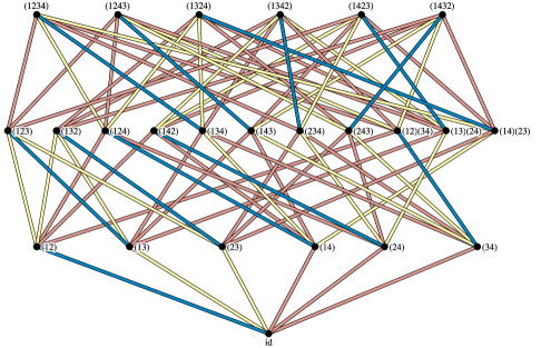
Figure 1. Edge labeled Cayley graph of $\mathrm{S}(4).$ Figure by M. LaCroix.

In order to visualize the coefficient of $\iota$ in (2.51), we consider the Cayley graph of $\mathrm{S}(d)$, as generated by the conjugacy class of transpositions. Let us mark each edge of the Cayley graph corresponding to the transposition $(s\ t)$ with $t,$ the larger of the two numbers interchanged. Figure 1 shows the case $d=4$, with $2$-edges in blue, $3$-edges in yellow, and $4$-edges in red. Let us call a walk on the Cayley graph monotone if the labels of the edges it traverses form a weakly increasing sequence. Thus, monotone walks are virtual histories of the evolution of a particle on $\mathrm{S}(d)$ which learns from experience — once it travels along an edge of value $t,$ it refuses to traverse edges of lesser value. Let $\vec{W}^{r}(\alpha,\beta)$ denote the number of monotone $r$-step walks on the Cayley graph which begin at a permutation of cycle type $\alpha$, and end at a permutation of cycle type $\beta$, i.e. the total number of monotone walks of length $r$ from the conjugacy class $C_{\alpha}$ to the conjugacy class $C_{\beta}$. Then, by definition of the complete symmetric polynomials and the Jucys-Murphy elements, we see that

(2.52) $$\langle\omega_{\alpha}f_{r}\omega_{\beta}\rangle=\vec{W}^{r}(\alpha,\beta).$$

Thus, Theorem 2.7 gives the following graphical expansion.

Theorem 2.8.

For any $1\leq d\leq N$, we have the absolutely convergent series expansions

$$\begin{split}I_{N}^{(0)d}&=N^{2d}\sum_{r=0}^{\infty}\left(-\frac{1}{N}\right)^{r}\vec{W}^{r}(1^{d},1^{d}),\\ I_{N}^{(1)d}&=N^{d}\sum_{\alpha\vdash d}p_{\alpha}(a_{1},\dots,a_{N})\sum_{r=0}^{\infty}\left(-\frac{1}{N}\right)^{r}\vec{W}^{r}(\alpha,1^{d}),\\ I_{N}^{(2)d}&=\sum_{\alpha,\beta\vdash d}p_{\alpha}(a_{1},\dots,a_{N})p_{\beta}(b_{1},\dots,b_{N})\sum_{r=0}^{\infty}\left(-\frac{1}{N}\right)^{r}\vec{W}^{r}(\alpha,\beta).\end{split}$$

Theorem 2.8 says that the stable string coefficients $I_{N}^{d}$ are generating functions for monotone walks on the symmetric group with endpoints in given conjugacy classes: with the case $m=0$ corresponds to loops based at a given point of $\mathrm{S}(d)$, the case $m=1$ corresponding to anchored walks issuing from the identity and ending in a given class, and the case $m=2$ allowing arbitrary conjugacy classes as boundary conditions. As a consistency check on the graphical expansion, observe that since

(2.53) $$\lim_{N\to\infty}\Omega_{\frac{1}{N}}(\lambda)=1$$

for each fixed $\lambda\vdash d$, we have

(2.54) $$\lim_{N\to\infty}\langle\omega_{\alpha}\Omega_{\frac{1}{N}}^{-1}\omega_{\beta}\rangle=\delta_{\alpha\beta}|C_{\alpha}|$$

for each fixed $\alpha,\beta\vdash d$, where the second equality is the orthogonality of irreducible characters. This comports with the combinatorially obvious enumeration of $0$-step walks from $C_{\alpha}$ to $C_{\beta}$,

(2.55) $$\vec{W}^{0}(\alpha,\beta)=\delta_{\alpha\beta}|C_{\alpha}|.$$

2.7. Topological expansion

The fact that monotone walks on symmetric groups play the role of Feynman diagrams for integration against the Haar measure on $\mathrm{U}(N)$ was discovered in [92], and further developed in [83, 84]. It was subsequently understood that these trajectories admit a natural topological interpretation involving branched covers of the sphere [50, 51].

To see this, let us recall the relationship between the number $W^{r}(\alpha,\beta)$ of not necessarily monotone $r$-step walks on $\mathrm{S}(d)$ between conjugacy classes $C_{\alpha}$ and $C_{\beta}$ and maps to the sphere. Applied in reverse, Hurwitz’s classical monodromy construction [67] interprets $\frac{1}{d!}W^{r}(\alpha,\beta)$ as a weighted count of isomorphism classes of pairs $(\mathbf{X},f)$ consisting of a compact Riemann surface $\mathbf{X}$ together with a degree $d$ holomorphic map $f\colon\mathbf{X}\to\mathbf{P}^{1}$ to the Riemann sphere with ramification profiles $\alpha,\beta$ over $\infty,0\in\mathbf{P}^{1}$, and the simplest non-trivial branching over the $r$th roots of unity on the sphere. The normalized counts $\frac{1}{d!}W^{r}(\alpha,\beta)$ were called the disconnected double Hurwitz numbers in [96]; for our purposes, it is more convenient to assign this name to the raw count $W^{r}(\alpha,\beta)$. By the Riemann-Hurwitz formula, the disconnected double Hurwitz number $W^{r}(\alpha,\beta)$ is zero unless

(2.56) $$r=2g-2+\ell(\alpha)+\ell(\beta),$$

where $g=g(\mathbf{X})$ is the genus of $\mathbf{X}$. Note that if

(2.57) $$\mathbf{X}=\mathbf{X}_{1}\sqcup\dots\sqcup\mathbf{X}_{c}$$

is a disjoint union of $c$ connected components, then

(2.58) $$g(\mathbf{X})=\left(g(\mathbf{X}_{1})-1\right)+\dots+\left(g(\mathbf{X}_{c})-1\right)+1$$

by additivity of the Euler characteristic, so that the genus of a disconnected surface may be negative but is subject to the lower bound

(2.59) $$g(\mathbf{X})\geq-c+1.$$

In view of (2.56), we may re-index the disconnected double Hurwitz numbers by genus, setting

(2.60) $$H_{g}^{\bullet}(\alpha,\beta):=W^{2g-2+\ell(\alpha)+\ell(\beta)}(\alpha,\beta),$$

where the bullet indicates disconnected. The case $\beta=1^{d}$ corresponds to covers unramified over $0\in\mathbf{P}^{1}$, and it is customary to write

(2.61) $$H_{g}^{\bullet}(\alpha):=H_{g}^{\bullet}(\alpha,1^{d})$$

and call these the disconnected single Hurwitz numbers; these were the numbers originally studied by Hurwitz [67, 68]. We may further define the disconnected simple Hurwitz numbers by

(2.62) $$H_{g}^{\bullet d}:=H_{g}^{\bullet}(1^{d}).$$

A good reference on the combinatorial features of simple Hurwitz numbers is [39].

By analogy with the above, the monotone walk counts $\vec{W}^{r}(\alpha,\beta)$ and $\vec{W}^{r}(\alpha,1^{d})$ were termed the disconnected monotone double and single Hurwitz numbers in [50, 51, 52]. Since these nonnegative integers are, by construction, smaller than their classical non-monotone counterparts, the Riemann-Hurwitz formula imposes the same vanishing condition on monotone Hurwitz numbers as it does on classical Hurwitz numbers, and accordingly we may re-index monotone Hurwitz numbers by genus, setting

(2.63) $$\vec{H}_{g}^{\bullet}(\alpha,\beta):=\vec{W}^{2g-2+\ell(\alpha)+\ell(\beta)}(\alpha,\beta)\quad\text{ and }\quad\vec{H}_{g}^{\bullet}(\alpha):=\vec{H}_{g}^{\bullet}(\alpha,1^{d}).$$

We further define the disconnected monotone simple Hurwitz numbers by

(2.64) $$\vec{H}_{g}^{\bullet d}:=\vec{H}_{g}^{\bullet}(1^{d}).$$

Topologically, monotone Hurwitz numbers may be viewed as corresponding to a signed enumeration of the the same class of covers counted by classical Hurwitz numbers; despite being signed, this count is always nonnegative. The classical and monotone constructions have been unified within a more general theory of weighted Hurwitz numbers [3], but remain the two most important and useful instances of this generalization. In particular, we may now interpret the graphical expansions given in Theorem 2.8 as topological expansions.

Theorem 2.9.

For any integers $1\leq d\leq N$, we have

$$I_{N}^{d}=\sum_{g=-d+1}^{\infty}N^{2-2g}I_{Ng}^{d},$$

where the series is $\|\cdot\|$-absolutely convergent, and the coefficients $I_{Ng}^{d}=I_{Ng}^{(m)d}$ are homogeneous degree $d$ polynomials in $mN$ variables given by

$$\begin{split}I_{N}^{(0)d}&=\vec{H}_{g}^{\bullet d},\\ I_{N}^{(1)d}&=\sum_{\alpha\vdash d}\frac{p_{\alpha}(a_{1},\dots,a_{N})}{N^{\ell(\alpha)}}(-1)^{\ell(\alpha)+d}\vec{H}_{g}^{\bullet}(\alpha),\\ I_{N}^{(2)d}&=\sum_{\alpha,\beta\vdash d}\frac{p_{\alpha}(a_{1},\dots,a_{N})}{N^{\ell(\alpha)}}\frac{p_{\beta}(b_{1},\dots,b_{N})}{N^{\ell(\beta)}}(-1)^{\ell(\alpha)+\ell(\beta)}\vec{H}_{g}^{\bullet}(\alpha,\beta).\end{split}$$

3. Infinite $N$

From Section 2, we know that for sufficiently strong coupling the large $N$ behavior of $I_{N}$ is captured by its critical coupling coefficients

(3.1) $$I_{N}^{1},\dots,I_{N}^{\lfloor tN^{2}\rfloor}.$$

However, only the first $N$ of these, the stable coupling coefficients

(3.2) $$I_{N}^{1},\dots,I_{N}^{N},$$

admit convergent topological expansions. We will bridge the gap between the stable and critical ranges analytically, as $N\to\infty$, in Section 4. In this section we do so formally, by setting $N=\infty$.

3.1. Stable partition functions

From the matrix integral perspective, setting $N=\infty$ in our problem corresponds to replacing the integrals (1.1) and (1.2) with

(3.3) $$I^{(1)}=\int_{\mathrm{U}}e^{\sqrt{z}\hbar^{-1}\operatorname{Tr}(AU+BU^{-1})}\mathrm{d}U,$$

and

(3.4) $$I^{(2)}=\int_{\mathrm{U}}e^{z\hbar^{-1}\operatorname{Tr}AUBU^{-1}}\mathrm{d}U,$$

where the integration is over the stable unitary group [14, 106]

(3.5) $$U=\varinjlim\mathrm{U}(N)$$

with $\hbar$ an infinitely small parameter and $A,B$ infinitely large matrices. However, as $\mathrm{U}$ is not locally compact and does not support a Haar measure, and these are ill-defined functional integrals.

Another approach to stability is to set $N=\infty$ in the coupling expansion of $I_{N}$, which means that we consider power series

(3.6) $$I^{(m)}=1+\sum_{d=1}^{\infty}\frac{z^{d}}{d!}I^{(m)d},\quad m=0,1,2$$

in a formal coupling constant $z$ whose coefficients $I^{(m)d}$ are themselves formal series in an indeterminate $\hbar$ representing the parameter $1/N$ at $N=\infty$. More precisely, the coupling coefficients $I^{(m)d}$ may be constructed as statistical expansions which are $N=\infty$ versions of the statistical expansions of $I_{N}^{(m)d}$ given by Theorem 2.7,

(3.7) $$\begin{split}I^{(0)d}&=\hbar^{-2d}\sum_{r=0}^{\infty}(-\hbar)^{r}\langle f_{r}\rangle\\ I^{(1)d}&=\hbar^{-d}\sum_{\alpha\vdash d}p_{\alpha}(A)\hbar^{-d}\sum_{r=0}^{\infty}(-\hbar)^{r}\langle\omega_{\alpha}f_{r}\rangle\\ I^{(2)d}&=\sum_{\alpha,\beta\vdash d}p_{\alpha}(A)p_{\beta}(B)\sum_{r=0}^{\infty}(-\hbar)^{r}\langle\omega_{\alpha}f_{r}\omega_{\beta}\rangle,\end{split}$$

or as graphical expansions which are $N=\infty$ versions of the graphical expansions of $I_{N}^{(m)d}$ given by Theorem 2.8,

(3.8) $$\begin{split}I^{(0)d}&=\hbar^{-2d}\sum_{r=0}^{\infty}(-\hbar)^{r}\vec{W}^{r}(1^{d},1^{d})\\ I^{(1)d}&=\hbar^{-d}\sum_{\alpha\vdash d}p_{\alpha}(A)\hbar^{-d}\sum_{r=0}^{\infty}(-\hbar)^{r}\vec{W}^{r}(\alpha,1^{d})\\ I^{(2)d}&=\sum_{\alpha,\beta\vdash d}p_{\alpha}(A)p_{\beta}(B)\sum_{r=0}^{\infty}(-\hbar)^{r}\vec{W}^{r}(\alpha,\beta),\end{split}$$

or as topological expansions which are $N=\infty$ versions of the topological expansions of $I_{N}^{(m)d}$ given by Theorem 2.8,

(3.9) $$\begin{split}I^{(0)d}&=\sum_{g=-d+1}\hbar^{2g-2}\vec{H}_{g}^{\bullet d}\\ I^{(1)d}&=\sum_{\alpha\vdash d}\frac{p_{\alpha}(A)}{\hbar^{-\ell(\alpha)}}(-1)^{\ell(\alpha)+d}\sum_{g=-d+1}^{\infty}\hbar^{2g-2}\vec{H}_{g}^{\bullet}(\alpha)\\ I^{(2)d}&=\sum_{\alpha\vdash d}\frac{p_{\alpha}(A)}{\hbar^{-\ell(\alpha)}}\frac{p_{\alpha}(B)}{\hbar^{-\ell(B)}}(-1)^{\ell(\alpha)+\ell(\beta)}\sum_{g=-d+1}^{\infty}\hbar^{2g-2}\vec{H}_{g}^{\bullet}(\alpha,\beta).\end{split}$$

Here

(3.10) $$p_{\alpha}(A)=\prod_{i=1}^{\ell(\alpha)}\sum_{j=1}^{\infty}a_{j}^{\alpha_{i}}\quad\text{ and }\quad p_{\beta}(B)=\prod_{i=1}^{\ell(\beta)}\sum_{j=1}^{\infty}b_{j}^{\beta_{i}}$$

are the Newton power sum symmetric functions in two countably infinite alphabets $A=\{a_{1},a_{2},\dots\}$ and $B=\{b_{1},b_{2},\dots\}$ of formal variables playing the role of the external matrix fields in the integrals (1.1) and (1.2). Observe that the signs which appear in these expressions could be eliminated simply by replacing $\hbar$ with $-\hbar$, but we refrain from doing this in order to maintain notational consistency with Section 2, and because we wish to emphasize that $\hbar$ is a formal replacement for $1/N$, not for $-1/N$. We view the generating functions $I^{(1)}$ and $I^{(2)}$ as meaningful algebraic versions of the ill-defined functional integrals (3.3) and (3.18).

3.2. Stable free energy

A subtle but important feature of the total generating function $I$ for disconnected monotone Hurwitz theory is that the variable $\hbar$ is an ordinary marker for Euler characteristic, whereas in classical Hurwitz theory one uses an exponential marker for this statistic [55, 96]. In a sense, this particularity explains the inevitability of monotone Hurwitz theory: the large $N$ expansion (1.4) presents as an ordinary generating function in $1/N$, not an exponential one, so that Hurwitz theory must be desymmetrized in order to match it with the ’t Hooft expansion. Crucially, we have the following theorem from [50, 51], which says that even though $I$ is a mixed ordinary/exponential generating function, taking the logarithm does indeed extract connected information.

Theorem 3.1.

We have

$$\log I^{(m)}=F^{(m)},$$

where

$$F^{(0)} =\sum_{d=1}^{\infty}\frac{z^{d}}{d!}\sum_{g=0}^{\infty}\hbar^{2g-2}\vec{H}_{g}^{d}$$

$$F^{(1)} =\sum_{d=1}^{\infty}\frac{z^{d}}{d!}\sum_{\alpha\vdash d}\frac{p_{\alpha}(A)}{\hbar^{-\ell(\alpha)}}(-1)^{\ell(\alpha)+d}\sum_{g=0}^{\infty}\hbar^{2g-2}\vec{H}_{g}(\alpha)$$

$$F^{(2)} =\sum_{d=1}^{\infty}\frac{z^{d}}{d!}\sum_{\alpha\vdash d}\frac{p_{\alpha}(A)}{\hbar^{-\ell(\alpha)}}\frac{p_{\alpha}(B)}{\hbar^{-\ell(B)}}(-1)^{\ell(\alpha)+\ell(\beta)}\sum_{g=0}^{\infty}\hbar^{2g-2}\vec{H}_{g}(\alpha,\beta).$$

are total generating functions for the connected monotone simple, single, and double Hurwitz numbers in all degrees and genera.

An immediate corollary of Theorem 3.1 is that a formal version of Conjecture 1.1 holds at $N=\infty$, i.e. the stable free energy $F=\log I$ admits a topological expansion.

Theorem 3.2.

We have

$$\log I=\sum_{g=0}^{\infty}\hbar^{2g-2}F_{g},$$

where

$$F_{g}^{(0)} =\sum_{d=1}^{\infty}\frac{z^{d}}{d!}\vec{H}_{g}^{d}$$

$$F_{g}^{(1)} =\sum_{d=1}^{\infty}\frac{z^{d}}{d!}\sum_{\alpha\vdash d}\frac{p_{\alpha}(A)}{\hbar^{-\ell(\alpha)}}(-1)^{\ell(\alpha)+d}\vec{H}_{g}(\alpha)$$

$$F_{g}^{(2)} =\sum_{d=1}^{\infty}\frac{z^{d}}{d!}\sum_{\alpha\vdash d}\frac{p_{\alpha}(A)}{\hbar^{-\ell(\alpha)}}\frac{p_{\alpha}(B)}{\hbar^{-\ell(B)}}(-1)^{\ell(\alpha)+\ell(\beta)}\vec{H}_{g}(\alpha,\beta).$$

are generating functions for the connected monotone simple, single, and double Hurwitz numbers in specified genus $g\geq 0$.

We emphasize that even this formal algebraic result has not previously appeared in the literature in this entirety. The case $m=2$ is implicit in [52]. The total generating function for monotone single Hurwitz numbers was studied in [50, 51] where low-genus explicit formulas and rational parameterizations were found, without the understanding that what was being analyzed was the stable free energy of the BGW model.

3.3. Topological expansion as topological factorization

Our approach to Conjecture 1.1 is based on converting the stable topological expansion of $F=\log I$ given by Theorem 3.2, which is purely algebraic, into an analytically meaninfgul $N\to\infty$ asymptotic expansion of $F_{N}=\log I_{N}$ which holds at sufficiently strong coupling. However, this cannot be done directly at the free energy level, since we do not know whether or not the stable nonvanishing hypothesis holds, and a priori it is not clear that we can view $F_{N}$ as an element of $\mathcal{O}_{N}(\delta)$ for $\delta>0$ an absolute constant. We therefore have to work with $I_{N}$ itself, and consequently it is beneficial to reformulate topological expansion of the stable free energy $F$ as topological factorization of the stable partition function $I$. More precisely, Theorem 3.2 is equivalent to the statement that, for each $k\in\mathbb{N}_{0}$, we have the factorization

(3.11) $$I=E_{\overline{k}}E_{\underline{k+1}},$$

where

(3.12) $$E_{\overline{k}}=e^{\sum_{g=0}^{k}\hbar^{2g-2}F_{g}}=1+\sum_{d=1}^{\infty}\frac{z^{d}}{d!}E_{\overline{k}}^{d}$$

and

(3.13) $$E_{\underline{k+1}}=e^{\sum_{g=k+1}^{\infty}\hbar^{2g-2}F_{g}}=1+\sum_{d=1}^{\infty}\frac{z^{d}}{d!}E_{\underline{k+1}}^{d}$$

are generating functions for disconnected covers built from connected components of genus at most $k$ and at least $k+1$, respectively. For example, in the notationally simplest case $m=0$, we have

(3.14) $$E_{\overline{k}}^{d}=\sum_{g=-d+1}^{\infty}\hbar^{2g-2}\vec{H}_{g\overline{k}}^{\bullet d}$$

with $\vec{H}_{g\overline{k}}^{\bullet d}$ the number of degree $d$ disconnected simple covers of genus $g$ all of whose connected components have genus at most $k$, while

(3.15) $$E_{\underline{k+1}}^{d}=\sum_{g=k+1}^{\infty}\hbar^{2g-2}\vec{H}_{g\underline{k+1}}^{\bullet d}$$

is a generating function for the number $\vec{H}_{g\underline{k+1}}^{\bullet d}$ of disconnected simple covers of genus $g$ all of whose connected components have genus at least $k+1$, and the sum starts at $g=k+1$ because any such cover must itself have genus $k+1$. At the level of coupling coefficients, Theorem 3.2 is equivalent to a binomial convolution formula describing the construction of an arbitrary degree $d$ cover as a shuffle of two smaller-degree disconnected covers built from connected components of genus at most $k$ and at least $k+1$, respectively.

Theorem 3.3.

For any $d\in\mathbb{N}$ and $k\in\mathbb{N}_{0}$, we have

$$I^{d}=\sum_{c=0}^{d}{d\choose c}E_{\overline{k}}^{c}E_{\underline{k+1}}^{d-c}.$$

3.4. Topological factorization as topological concentration

Viewing the stable partition function $I$ as a formal replacement for an infinite-dimensional functional integral (e.g. (3.3) or (3.18)), it is natural to further recast the topological factorization (3.11) as a “concentration inequality” for the corresponding integral. More precisely, let us define the $k$th order topological normalization of the stable partition function $I$ to be the series

(3.16) $$\Phi_{k}=E_{\underline{k}}^{-1}I.$$

In the case $m=1$, this is a formal replacement for the topological normalization of the stable BGW integral,

(3.17) $$\Phi_{k}^{(1)}=e^{-\sum_{g=0}^{k}\hbar^{2g-2}F_{g}^{(1)}}\int_{\mathrm{U}}e^{\sqrt{z}\hbar^{-1}\operatorname{Tr}(AU+BU^{-1})}\mathrm{d}U,$$

and in the case $m=2$ it is a formal algebraic version of the topologically normalized HCIZ integral,

(3.18) $$\Phi_{k}^{(2)}=e^{-\sum_{g=0}^{k}\hbar^{2g-2}F_{g}^{(2)}}\int_{\mathrm{U}}e^{z\hbar^{-1}\operatorname{Tr}AUBU^{-1}}\mathrm{d}U.$$

The topological factorization of $I$ is then equivalent to the identity

(3.19) $$\Phi_{k}=E_{\underline{k+1}},$$

which at the level of coupling coefficients is equivalent to the “topological cancellation” identity

(3.20) $$\Phi_{k}^{d}=\sum_{c=0}^{d}{d\choose c}I^{c}(E_{k}^{-1})^{d-c}=E_{k+1}^{d},$$

where

(3.21) $$E_{k}^{-1}=e^{-\sum_{g=0}^{k}\hbar^{2g-2}F_{g}}=1+\sum_{d=1}^{\infty}\frac{z^{d}}{d!}(E_{k}^{-1})^{d}$$

the coupling expansion of the topological normalization factor $E_{k}^{-1}$. Since $E_{\underline{k+1}}$ is a generating function for covers built from connected components of genus at least $k+1$, this implies the algebraic concentration inequality

(3.22) $$\Phi_{k}-1=O(\hbar^{2k}),$$

We will see in Section 4 that proving Conjecture 1.1 can be reduced to establishing an $N\to\infty$ version of (3.22) which holds at sufficiently strong coupling.

3.5. Summability in fixed genus

The following theorem from [54] forms the bridge between the stable world of formal power series and the analytic world of holomorphic functions.

Theorem 3.4.

For each $g\in\mathbb{N}_{0}$, the generating function $F_{g}^{(0)}$ for connected monotone simple Hurwitz numbers of genus $g$ has radius of convergence equal to $2/27$.

Theorem 3.4 is deduced in [54] from the results of [51], which imply that the series $F_{g}^{(0)}$ can be expressed in terms of the classical Gaussian hypergeometric function. Interestingly, the constant $2/27$ also appears in the asymptotic enumeration of finite groups [100]. For other appearances of $2/27$ see [72] and [25], the latter reference being more directly (but still not transparently) related to the present context.

Theorem 3.4 can be lifted to summability of the analogous genus-specific generating functions for the connected single and double monotone Hurwitz numbers, via the connected version of Theorem 3.7, also proved in [54].

Theorem 3.5.

For any $d\in\mathbb{N}$ and $g\in\mathbb{N}_{0}$, we have nd the same relation holds in the connected case,

$$\sum_{\alpha,\beta\vdash d}\vec{H}_{g}(\alpha,\beta)<2^{d}\sum_{\alpha\vdash d}\vec{H}_{g}(\alpha)<4^{d}\vec{H}_{g}^{d}.$$

3.6. Large genus asymptotics

Theorem 3.4 corresponds to an asymptotic result for the connected monotone simple Hurwitz numbers in the large degree limit: for each fixed $g\in\mathbb{N}_{0}$, we have

(3.23) $$\frac{1}{d!}\vec{H}_{g}^{d}\sim t_{g}(d)\left(\frac{27}{2}\right)^{d},\quad d\to\infty,$$

with $t_{g}(d)$ a genus-dependent factor of sub-exponential growth in $d$. Below, we will also need information on the large genus asymptotics of disconnected monotone simple Hurwitz numbers in fixed degree. These asymptotics are as follows.

Theorem 3.6.

For any $d\in\mathbb{N}$, we have

$$\vec{H}_{g}^{\bullet d}\sim\frac{2(d-1)^{3d-3}}{(d-1)!d!}(d-1)^{2g},\quad g\to\infty.$$

Proof.

Let $d\in\mathbb{N}$ be arbitrary but fixed. Since $\vec{H}_{g}^{\bullet d}=\vec{W}^{2g-2+2d}(1^{d},1^{d})$, the $g\to\infty$ asymptotic behavior of the monotone Hurwitz number $\vec{H}_{g}^{\bullet d}$ is equivalent to the $r\to\infty$ asymptotic behavior of the monotone loop counts $\vec{W}^{r}(1^{d},1^{d})$.

From Section 2, we know that the ordinary generating function for monotone loops $\vec{W}^{r}(1^{d},1^{d})$ based at a given point of the symmetric group is a rational function of $\hbar$,

(3.24) $$\sum_{r=0}^{\infty}\hbar^{r}\vec{W}^{r}(1^{d},1^{d})=\sum_{\lambda\vdash d}\frac{(\dim\mathsf{V}^{\lambda})^{2}}{d!}\prod_{\Box\in\lambda}\frac{1}{1-\hbar c(\Box)}.$$

It follows that, as a function of $r$, the loop count $\vec{W}^{r}(1^{d},1^{d})$ is a linear combination of the exponential functions

(3.25) $$1^{r},2^{r},\dots,(d-1)^{r}$$

whose coefficients are polynomials in $r$. In other words, $\vec{W}^{r}(1^{d},1^{d})$ is a quasipolynomial function of $r$. The dominant term of this quasipolynomial comes from those terms in the Plancherel average which have one of the factors $(1-(d-1)\hbar)$ or $(1+(d-1)\hbar)$ in their denominator, and the only two terms which meet this condition correspond to the trivial representation,

(3.26) $$\frac{1}{d!}\frac{1}{(1-\hbar)(1-2\hbar)\dots(1-(d-1)\hbar)}=\frac{1}{d!}\sum_{r=0}^{\infty}\hbar^{r}f_{r}(1,2,\dots,(d-1)),$$

and the sign representation,

(3.27) $$\frac{1}{d!}\frac{1}{(1+\hbar)(1+2\hbar)\dots(1+(d-1)\hbar)}=\frac{1}{d!}\sum_{r=0}^{\infty}\hbar^{r}f_{r}(-1,-2,\dots,-(d-1)),$$

so that by homogeneity we have

(3.28) $$\vec{W}^{r}(1^{d},1^{d})\sim\frac{1^{r}+(-1)^{r}}{d!}f_{r}(1,\dots,d-1),\quad r\to\infty.$$

Specializing the complete symmetric functions at consecutive positive integers yields Stirling numbers of the second kind [81], and in particular we have

(3.29) $$f_{r}(1,2,\dots,d-1)=\genfrac{\{}{\}}{0.0pt}{}{d-1+r}{d-1}.$$

The asymptotic behavior of Stirling numbers with large upper index and fixed lower index is also known [89], and in particular we have

(3.30) $$\genfrac{\{}{\}}{0.0pt}{}{d-1+r}{d-1}\sim\frac{(d-1)^{d-1}}{(d-1)!}(d-1)^{r},\quad r\to\infty.$$

Taking $r=2g-2+2d$, we obtain

(3.31) $$\vec{W}^{r}(1^{d},1^{d})\sim\frac{(1^{r}+(-1)^{r})(d-1)^{d-1}}{(d-1)!d!}(d-1)^{r},\quad r\to\infty$$

and

(3.32) $$\vec{H}_{g}^{\bullet d}\sim\frac{2(d-1)^{3d-3}}{(d-1)!d!}(d-1)^{2g},\quad g\to\infty,$$

as claimed. ∎

It is interesting to compare the asymptotics of monotone simple Hurwitz numbers catalogued here with those of classical simple Hurwitz numbers, which are clearly catalogued in [39]. We end this section by remarking that the disconnnected version of the Theorem 3.5 also holds; the proof is identical to the connected case.

Theorem 3.7.

For any $d\in\mathbb{N}$ and $g\in\mathbb{Z}$, we have

$$\sum_{\alpha,\beta\vdash d}\vec{H}_{g}^{\bullet}(\alpha,\beta)<2^{d}\sum_{\alpha\vdash d}\vec{H}_{g}^{\bullet}(\alpha)<4^{d}\vec{H}_{g}^{\bullet d}.$$

4. Large $N$

In this Section, we combine the theorems of Sections 2 and 3 with complex analytic methods to prove a generalization of Theorem 1.2, which in particular confirms Conjecture 1.1. More precisely, we are concerned with the $N\to\infty$ asymptotics of the triarchy of entire functions in $mN+1$ complex variables defined by

(4.1) $$I_{N}^{(m)}=1+\sum_{d=1}^{\infty}\frac{z^{d}}{d!}I_{N}^{(m)d},\quad m\in\{0,1,2\},\ N\in\mathbb{N},$$

whose coupling coefficients may be described in character form,

(4.2) $$\begin{split}I_{N}^{(0)d}&=N^{2d}\sum_{\begin{subarray}{c}\lambda\vdash d\\ \ell(\lambda)\leq N\end{subarray}}\prod_{\Box\in\lambda}\frac{1}{h(\Box)^{2}(1+\frac{c(\Box)}{N})},\\ I_{N}^{(1)d}&=N^{d}\sum_{\begin{subarray}{c}\lambda\vdash d\\ \ell(\lambda)\leq N\end{subarray}}s_{\lambda}(a_{1},\dots,a_{N})\prod_{\Box\in\lambda}\frac{1}{h(\Box)(1+\frac{c(\Box)}{N})},\\ I_{N}^{(2)d}&=\sum_{\begin{subarray}{c}\lambda\vdash d\\ \ell(\lambda)\leq N\end{subarray}}s_{\lambda}(a_{1},\dots,a_{N})s_{\lambda}(b_{1},\dots,b_{N})\prod_{\Box\in\lambda}\frac{1}{1+\frac{c(\Box)}{N}},\end{split}$$

or equivalently in string form,

(4.3) $$\begin{split}I_{N}^{(0)d}&=N^{2d}\sum_{\begin{subarray}{c}\lambda\vdash d\\ \ell(\lambda)\leq N\end{subarray}}\Omega_{\frac{1}{N}}^{-1}(\lambda)\frac{(\dim\mathsf{V}^{\lambda})^{2}}{d!},\\ I_{N}^{(1)d}&=N^{d}\sum_{\alpha\vdash d}p_{\alpha}(a_{1},\dots,a_{N})\sum_{\begin{subarray}{c}\lambda\vdash d\\ \ell(\lambda)\leq N\end{subarray}}\omega_{\alpha}(\lambda)\Omega_{\frac{1}{N}}^{-1}(\lambda)\frac{(\dim\mathsf{V}^{\lambda})^{2}}{d!},\\ I_{N}^{(2)d}&=\sum_{\alpha\vdash d}p_{\alpha}(a_{1},\dots,a_{N})p_{\beta}(b_{1},\dots,b_{N})\sum_{\begin{subarray}{c}\lambda\vdash d\\ \ell(\lambda)\leq N\end{subarray}}\omega_{\alpha}(\lambda)\Omega_{\frac{1}{N}}^{-1}(\lambda)\omega_{\beta}(\lambda)\frac{(\dim\mathsf{V}^{\lambda})^{2}}{d!}.\end{split}$$

We continue the practice of omitting the superscript $m$ when making statements which hold uniformly in $m\in\{0,1,2\}$, when it is convenient to do so.

Our goal is to obtain $N\to\infty$ asymptotics for $F_{N}^{(m)}=\log I_{N}^{(m)}$ on the closed origin-centered polydisc $\mathbf{D}_{N}(\varepsilon)$ of polyradius $(\varepsilon,1,\dots,1)$ in $\mathbb{C}^{mN+1}$, with $\varepsilon>0$ a sufficiently small absolute constant. At present, we do not know that this is a well-defined objective, as there may be no $\varepsilon>0$ such that $F_{N}^{(m)}$ is defined and analytic on $\mathbf{D}_{N}(\varepsilon)$, i.e. we do not know that the stable nonvanishing hypothesis holds. However, Section 3 gives us explicit analytic targets, and also places a limitation on how large $\varepsilon$ can be. Let $\gamma\in(0,\frac{1}{54})$ be fixed for the rest of the paper. Then, by the results of Section 3, for each $N\in\mathbb{N}$, the power series

(4.4) $$F_{Ng}^{(m)}=\sum_{d=1}^{\infty}\frac{z^{d}}{d!}F_{Ng}^{(m)d},\quad g\in\mathbb{N}_{0},\ m\in\{0,1,2\}$$

whose coefficients are the polynomials in $mN$ variables defined by

(4.5) $$\begin{split}F_{Ng}^{(0)d}&=\vec{H}_{g}^{d}\\ F_{Ng}^{(1)d}&=\sum_{\alpha\vdash d}\frac{p_{\alpha}(a_{1},\dots,a_{N})}{N^{\ell(\alpha)}}(-1)^{\ell(\alpha)+d}\vec{H}_{g}(\alpha),\\ F_{Ng}^{(2)d}&=\sum_{\alpha,\beta\vdash d}\frac{p_{\alpha}(a_{1},\dots,a_{N})}{N^{\ell(\alpha)}}\frac{p_{\beta}(b_{1},\dots,b_{N})}{N^{\ell(\beta)}}(-1)^{\ell(\alpha)+\ell(\beta)}\vec{H}_{g}(\alpha,\beta)\end{split}$$

are $\|\cdot\|_{\gamma}$-absolutely convergent, i.e. are members of $\mathcal{O}_{N}(\gamma)$, and

(4.6) $$\sup_{N\in\mathbb{N}}\|F_{Ng}\|_{\gamma}<\infty$$

by construction.

In this Section, we prove the following theorem.

Theorem 4.1.

There exists $\varepsilon\in(0,\gamma)$ such that $I_{N}^{(m)}$ is non-vanishing on $\mathbf{D}_{N}(\varepsilon)$ for all $N\in\mathbb{N}$, and such that $F_{N}^{(m)}=\log I_{N}^{(m)}$ satisfies

$$\lim_{N\to\infty}N^{2k-2}\left\|F_{N}^{(m)}-\sum_{g=0}^{k}N^{2-2g}F_{Ng}^{(m)}\right\|_{\varepsilon}=0$$

for each fixed $k\in\mathbb{N}_{0}$.

4.1. Large $N$ expansion

For each $N\in\mathbb{N}$, let $\rho_{N}>0$ be such that the entire function $I_{N}$ is non-vanishing on the closed origin-centered polydisc $\mathbf{D}_{N}(\rho_{N})$. Note that we are not assuming the positive sequence $(\rho_{N})_{N=1}^{\infty}$ can be selected such that it has positive infimum, i.e. we are not assuming that the stable non-vanishing hypothesis holds.

For each $N\in\mathbb{N}$, the free energy $F_{N}=\log I_{N}$ is analytic on an open neighborhood of $\mathbf{D}_{N}(\rho_{N})$, and its Maclaurin series

(4.7) $$F_{N}^{d}=\sum_{d=1}^{\infty}\frac{z^{d}}{d!}F_{N}^{d},$$

converges uniformly absolutely on $\mathbf{D}_{N}(\rho_{N})$.

Theorem 4.2.

For any $1\leq d\leq N$, we have

$$F_{N}^{d}=\sum_{g=0}^{\infty}N^{2-2g}F_{Ng}^{d}$$

where the series converges $\|\cdot\|$-absolutely and $F_{Ng}^{d}$ is the polynomial (4.5).

Proof.

This follows immediately from Theorem 2.9 together with Theorem 3.1. ∎

Theorem 4.2 yields the large $N$ expansion (aka genus expansion or ‘t Hooft expansion) of each fixed strong coupling coefficient $F_{N}^{d}$, as defined by (1.5).

Theorem 4.3.

For each fixed $d\in\mathbb{N}$ and $k\in\mathbb{N}_{0}$, we have

$$\lim_{N\to\infty}N^{2k-2}\left\|F_{N}^{d}-\sum_{g=0}^{k}N^{2-2g}F_{Ng}^{d}\right\|=0$$

Proof.

Let $d\in\mathbb{N}$ and $k\in\mathbb{N}_{0}$ be fixed. By Theorem 4.2, for any $N\geq d$ we have

$$F_{N}^{d}-\sum_{g=0}^{k}N^{2-2g}F_{Ng}^{d}=\sum_{g=k+1}^{\infty}N^{2-2g}F_{Ng}^{d}.$$

Moreover, by Theorem 3.5 we have

(4.8) $$\|F_{Ng}^{d}\|<4^{d}\vec{H}_{g}^{d}.$$

We thus have

$$N^{2k-2}\left\|F_{N}^{d}-\sum_{g=0}^{k}N^{2-2g}F_{Ng}^{d}\right\|<4^{d}\sum_{l=1}^{\infty}N^{-2l}\vec{H}_{k+l}^{d}<\infty$$

for any $N\geq d$. Since the upper bound is positive and strictly decreasing in $N$, the result follows from the monotone convergence theorem. ∎

4.2. Cancellation scheme

The fact that monotone Hurwitz numbers are the combinatorial invariants underlying the large $N$ expansion of the strong coupling coefficients $F_{N}^{d}$ of the HCIZ and BGW integrals has implications in both directions. In particular, it implies the following cancellation feature of monotone Hurwitz numbers, which classical Hurwitz numbers do not share. We shall use this cancellation scheme below.

Theorem 4.4.

For any $(d,g)\in\mathbb{N}\times\mathbb{N}_{0}$ except $(1,0)$, we have

$$\sum_{\beta\vdash d}(-1)^{\ell(\beta)}\vec{H}_{g}(\alpha,\beta)=0$$

for all $\alpha\vdash d$.

Proof.

The case where $d=1$ and $g>0$ is combinatorially obvious: the sum consists of the single term $\vec{H}_{g}(1,1)$, which vanishes as there are no walks of positive length in a graph with a single vertex.

For $d>1$, the cancellation identity is obtained by turning off one of the two external fields in the HCIZ integral and appealing to Theorems 4.2 and 4.3. More precisely, we consider the specialization of $I_{N}$ in which $B$ is the identity matrix. The character form of $I_{N}^{(1)d}$ then degenerates to

(4.9) $$I_{N}^{d}=N^{d}\sum_{\begin{subarray}{c}\lambda\vdash d\\ \ell(\lambda)\leq N\end{subarray}}s_{\lambda}(a_{1},\dots,a_{N})\dim\mathsf{V}^{\lambda}=N^{d}p_{1^{d}}(a_{1},\dots,a_{N}),$$

so that $I_{N}$ itself degenerates to the exponential function

(4.10) $$I_{N}=e^{zNp_{1}(a_{1},\dots,a_{N})},$$

a fact which is also obvious from the integral representation (1.2). The free energy $F_{N}=\log I_{N}$ in this degeneration is simply the polynomial $F_{N}=zNp_{1}(a_{1},\dots,a_{N})$, so the strong coupling coefficients are

(4.11) $$F_{N}^{1}=N^{2}\frac{p_{1}(a_{1},\dots,a_{N})}{N}$$

and $F_{N}^{d}=0$ for $d>1$. Thus by Theorem 4.2, for any $1<d\leq N$ we have that

(4.12) $$\sum_{\alpha\vdash d}\frac{p_{\alpha}(a_{1},\dots,a_{N})}{N^{\ell(\alpha)}}(-1)^{\ell(\alpha)}\sum_{\beta\vdash d}(-1)^{\ell(\beta)}\sum_{g=0}^{\infty}N^{2-2g}\vec{H}_{g}(\alpha,\beta)=0,$$

which yields

(4.13) $$\sum_{\beta\vdash d}(-1)^{\ell(\beta)}\sum_{g=0}^{\infty}N^{-2g}\vec{H}_{g}(\alpha,\beta)=0$$

for all $\alpha\vdash d$, by linear independence of the Newton polynomials

(4.14) $$p_{\alpha}(x_{1},\dots,x_{N}),\quad\alpha\vdash d$$

in the stable range $1\leq d\leq N$.

We now proceed by induction in $g$. For $g=0$, take the $N\to\infty$ limit in (4.13) to obtain

(4.15) $$\sum_{\beta\vdash d}(-1)^{\ell(\beta)}\vec{H}_{0}(\alpha,\beta)=0$$

for all $\alpha\vdash d$. Assuming the result holds up to genus $k$, (4.13) becomes

(4.16) $$\sum_{\beta\vdash d}(-1)^{\ell(\beta)}\sum_{g=k+1}^{\infty}N^{-2g}\vec{H}_{g}(\alpha,\beta)=0,$$

for all $\alpha\vdash d$. Multiply (4.16) by $N^{2k}$ and take the $N\to\infty$ limit to obtain

(4.17) $$\sum_{\beta\vdash d}(-1)^{\ell(\beta)}\vec{H}_{k+1}(\alpha,\beta)=0$$

for all $\alpha\vdash d$.

∎

Remark 4.5.

When $\alpha=d$ is the Young diagram consisting of a single row of $d$ cells, we have the product formula

(4.18) $$\vec{H}_{0}(d,\beta)=\prod_{i=1}^{\ell(\beta)}\operatorname{Cat}_{\beta_{i}-1},$$

where $\operatorname{Cat}_{k}=\frac{1}{k+1}{2k\choose k}$ is the Catalan number [84]. Thus in the case $\alpha=d$ and $g=0$, Theorem 1.2 becomes

(4.19) $$\sum_{\beta\vdash d}(-1)^{\ell(\beta)}\operatorname{Cat}_{\beta_{i}-1}=0,$$

which is just the vanishing identity for the summation of the Mobius function of a poset in the case of the lattice of noncrossing partitions of $\{1,\dots,d\}$; see e.g. [90]. Probably, Theorem 4.4 is indicative of a relationship between monotone Hurwitz numbers and Mobius functions of higher genus noncrossing partitions.

4.3. Reduction to uniform boundedness

With Theorem 4.3 in hand, the proof of Theorem 4.1 reduces to establishing stable nonvanishing together with uniform boundedness. More precisely, we have the following reduction.

Theorem 4.6.

Suppose there exists $\delta\in(0,\gamma]$ such that $I_{N}$ is nonvanishing on $\mathbf{D}_{N}(\delta)$ for all $N\in\mathbb{N}$, and set $F_{N}=\log I_{N}\in\mathcal{O}_{N}(\delta)$. If for each $k\in\mathbb{N}_{0}$ we have

$$\left\|F_{N}-\sum_{g=0}^{k}N^{2-2g}F_{Ng}\right\|_{\delta}\leq M_{k}N^{2-2k}$$

for all $N\geq N_{k}$ sufficiently large, where $M_{k}\geq 0$ depends only on $k$, then Theorem 4.1 holds.

Proof.

Since $F_{Ng}\in\mathcal{O}_{N}(\gamma)$ for all $g\in\mathbb{N}_{0}$ and $\delta\leq\gamma$ the differences

(4.20) $$\Delta_{Nk}=F_{N}-\sum_{g=0}^{k}N^{2-2g}F_{Ng},\quad k\in\mathbb{N}_{0},$$

belong to the Banach algebra $\mathcal{O}_{N}(\delta)$. Let

(4.21) $$\Delta_{Nk}=\sum_{d=1}^{\infty}\frac{z^{d}}{d!}\Delta_{Nk}^{d}$$

be the coupling expansion of this holomorphic difference, so that

(4.22) $$\Delta_{Nk}^{d}=F_{N}^{d}-\sum_{g=0}^{k}N^{2-2g}F_{Ng}^{d},$$

and Theorem 4.3 says that

(4.23) $$\lim_{N\to\infty}N^{2k-2}\|\Delta_{Nk}^{d}\|=0.$$

Now fix $k\in\mathbb{N}_{0}$ and $\varepsilon<\delta,$ and let $\kappa>0$ be given. Under the hypothesis that $\|\Delta_{Nk}\|_{\delta}\leq M_{k}N^{2-2k}$ for all $N\geq N_{k}$ sufficiently large, where $M_{k}\geq 0$ depends only on $k$, we will prove that in fact

(4.24) $$\|\Delta_{Nk}\|_{\varepsilon}\leq\kappa N^{2-2k}$$

for all $N$ sufficiently large.

For any $N\in\mathbb{N}$, we have that

(4.25) $$\|\Delta_{Nk}\|_{\varepsilon}\leq\sum_{d=1}^{n}\frac{\varepsilon^{d}}{d!}\|\Delta_{Nk}^{d}\|+\sum_{d=n+1}^{\infty}\frac{\varepsilon^{d}}{d!}\|\Delta_{Nk}^{d}\|$$

for all $n\in\mathbb{N}$. By Cauchy’s estimate, for each $d\in\mathbb{N}$ we have

(4.26) $$\frac{\|\Delta_{Nk}^{d}\|}{d!}\leq\frac{\|\Delta_{Nk}\|_{\delta}}{\delta^{d}},$$

and thus

(4.27) $$\left\|\Delta_{Nk}\right\|_{\varepsilon}\\ \leq\ \sum_{d=1}^{n}\frac{\varepsilon^{d}}{d!}\|\Delta_{Nk}^{d}\|+\left(\frac{\varepsilon}{\delta}\right)^{n+1}\frac{M_{k}}{1-\frac{\varepsilon}{\delta}}N^{2-2k},$$

holds for each $n\in\mathbb{N}$, for all $N\geq N_{k}$. Consequently, for all $N\geq N_{k}$ sufficiently large we have that

(4.28) $$\left\|\Delta_{Nk}\right\|_{\varepsilon}\leq\ \sum_{d=1}^{n_{0}}\frac{\varepsilon^{d}}{d!}\|\Delta_{Nk}^{d}\|+\frac{\kappa}{2}N^{2-2k},$$

where $n_{0}$ is sufficiently large so that

(4.29) $$\left(\frac{\varepsilon}{\delta}\right)^{n_{0}+1}\frac{M_{k}}{1-\frac{\varepsilon}{\delta}}\leq\frac{\kappa}{2}.$$

Invoking Theorem 4.3, for $N$ sufficiently large we have

(4.30) $$\sum_{d=1}^{n_{0}}\frac{\varepsilon^{d}}{d!}\|\Delta_{Nk}^{d}\|=N^{2-2k}\sum_{d=1}^{n_{0}}\frac{\varepsilon^{d}}{d!}N^{2k-2}\|\Delta_{Nk}^{d}\|\leq N^{2-2k}\frac{\kappa}{2}$$

and we conclude that

(4.31) $$\left\|\Delta_{N}\right\|_{\varepsilon}\leq\kappa N^{2-2k},$$

holds for $N$ sufficiently large, as required.

∎

4.4. Reduction to concentration

We now show that the proof of Theorem 4.1 can be further reduced to establishing a large $N$ version of the $N=\infty$ topological concentration inequalities (3.22) for the stable integrals $I$.

For each $k\in\mathbb{N}_{0}$, we define $E_{N\overline{k}}\in\mathcal{O}_{N}(\gamma)$ by

(4.32) $$E_{N\overline{k}}=e^{\sum_{g=0}^{k}N^{2-2g}F_{Ng}}.$$

Then

(4.33) $$E_{N\overline{k}}=1+\sum_{d=1}^{\infty}\frac{z^{d}}{d!}E_{N\overline{k}}^{d},$$

where

(4.34) $$\begin{split}E_{N\overline{k}}^{(0)d}&=\sum_{g=-d+1}^{\infty}N^{2-2g}\vec{H}_{g\overline{k}}^{\bullet d},\\ E_{N\overline{k}}^{(1)d}&=\sum_{g=-d+1}^{\infty}N^{2-2g}\sum_{\alpha\vdash d}\frac{p_{\alpha}(a_{1},\dots,a_{N})}{N^{\ell(\alpha)}}(-1)^{\ell(\alpha)+d}\vec{H}_{g\overline{k}}^{\bullet}(\alpha),\\ E_{N\overline{k}}^{(2)d}&=\sum_{g=-d+1}^{\infty}N^{2-2g}\sum_{\alpha,\beta\vdash d}\frac{p_{\alpha}(a_{1},\dots,a_{N})}{N^{\ell(\alpha)}}\frac{p_{\beta}(b_{1},\dots,b_{N})}{N^{\ell(\beta)}}(-1)^{\ell(\alpha)+\ell(\beta)}\vec{H}_{g\overline{k}}^{\bullet}(\alpha,\beta),\end{split}$$

is a genus expansion for degree $d$ disconnected covers built from connected components of genus at most $k$ which converges uniformly absolutely on compact subsets of $\mathbb{C}^{mN}$, for all $d\in\mathbb{N}$. In particular, we have

(4.35) $$\|E_{N\overline{k}}^{d}\|=N^{2d}\left(1+O_{k}\left(\frac{1}{N}\right)\right).$$

Note that, in the stable range $1\leq d\leq N$, the complementary genus expansions

(4.36) $$\begin{split}E_{N\underline{k+1}}^{(0)d}&=\sum_{g=k+1}^{\infty}N^{2-2g}\vec{H}_{g\underline{k+1}}^{\bullet d},\\ E_{N\underline{k+1}}^{(1)d}&=\sum_{g=k+1}^{\infty}N^{2-2g}\sum_{\alpha\vdash d}\frac{p_{\alpha}(a_{1},\dots,a_{N})}{N^{\ell(\alpha)}}(-1)^{\ell(\alpha)+d}\vec{H}_{g\underline{k+1}}^{\bullet}(\alpha),\\ E_{N\underline{k+1}}^{(2)d}&=\sum_{g=k+1}^{\infty}N^{2-2g}\sum_{\alpha,\beta\vdash d}\frac{p_{\alpha}(a_{1},\dots,a_{N})}{N^{\ell(\alpha)}}\frac{p_{\beta}(b_{1},\dots,b_{N})}{N^{\ell(\beta)}}(-1)^{\ell(\alpha)+\ell(\beta)}\vec{H}_{g\underline{k+1}}^{\bullet}(\alpha,\beta),\end{split}$$

enumerating disconnnected degree $d$ covers assembled from connected components of genus at least $k+1$ converge uniformly absolutely on compact subsets of $\mathbb{C}^{mN}$, by Theorem 2.9 and the fact that $\vec{H}_{g\underline{k+1}}^{\bullet}(\alpha,\beta)\leq\vec{H}_{g}^{\bullet}(\alpha,\beta)$. However, the generating series for disconnected covers built from connected components of unbounded genus are divergent in the unstable range $d>N$.

For each $k\in\mathbb{N}_{0}$, define $\Phi_{Nk}\in\mathcal{O}_{N}(\gamma)$ by

(4.37) $$\Phi_{Nk}=E_{N\overline{k}}^{-1}I_{N}.$$

In the case $m=1$,

(4.38) $$\Phi_{Nk}^{(1)}=e^{-\sum_{g=0}^{k}N^{2-2g}F_{Ng}^{(1)}}\int_{\mathrm{U}(N)}e^{\sqrt{z}N\mathrm{Tr}(AU+BU^{-1})}\mathrm{d}U$$

is the $k$th order topological normalization of the BGW integral $I_{N}^{(1)}$, while in the case $m=2$

(4.39) $$\Phi_{Nk}^{(2)}=e^{-\sum_{g=0}^{k}N^{2-2g}F_{Ng}^{(2)}}\int_{\mathrm{U}(N)}e^{zN\mathrm{Tr}AUBU^{-1}}\mathrm{d}U$$

is the $k$th order topological normalization of the HCIZ integral $I_{N}^{(2)}$.

Theorem 4.7.

If there exists a constant $\xi\in(0,\gamma]$ such that for each $k\in\mathbb{N}_{0}$ we have

$$\|\Phi_{Nk}-1\|_{\xi}\leq C_{k}N^{2-2k}$$

for all $N\geq N_{k}$ sufficiently large, where $C_{k}\geq 0$ depends only on $k$, then Theorem 4.1 holds.

Proof.

By hypothesis, we have

(4.40) $$\|\Phi_{N2}-1\|_{\xi}\leq C_{2}N^{-2}$$

for all $N\geq N_{2}$ sufficiently large. This implies that

(4.41) $$\|\Phi_{N2}-1\|_{\xi}<1$$

for all $N>N_{0}:=\max(N_{2},\sqrt{C_{2}})$ sufficiently large, and hence that $\Phi_{N2}$ is non-vanishing on $\mathbf{D}_{N}(\xi)$ for all $N>N_{0}$. But

(4.42) $$\Phi_{N2}=e^{-(N^{2}F_{N0}+N^{0}F_{N1}+N^{-2}F_{N2})}I_{N}$$

is the product of a non-vanishing function and $I_{N}$, so that $I_{N}$ must be nonvanishing on $\mathbf{D}_{N}(\xi)$ for all $N>N_{0}$. Consequently, there is $\eta\in(0,\xi]$ such that $I_{N}$ is nonvanishing on $\mathbf{D}_{N}(\eta)$ for all $N\in\mathbb{N}$, whence $F_{N}=\log I_{N}$ is a well-defined member of $\mathcal{O}_{N}(\eta)$ for all $N\in\mathbb{N}$.

Now let $k\in\mathbb{N}_{0}$ be arbitrary but fixed. Since $\eta\leq\xi\leq\gamma$, the difference

(4.43) $$\Delta_{Nk}=F_{N}-\sum_{g=0}^{k}N^{2-2g}F_{Ng}$$

belongs to $\mathcal{O}_{N}(\eta)$ for all $N\in\mathbb{N}$. Now

(4.44) $$\|e^{\Delta_{Nk}}-1\|_{\eta}=\|\Phi_{Nk}-1\|_{\eta}\leq\|\Phi_{Nk}-1\|_{\xi},$$

so that by hypothesis we have

(4.45) $$\|e^{\Delta_{Nk}}-1\|_{\eta}\leq C_{k}N^{2-2k}$$

for all $N\geq N_{k}$ sufficiently large.

For the rest of the argument, we assume $N\geq N_{k}$. From the above we have that $e^{\Delta_{Nk}}$ belongs to the closed unit ball of radius $C_{k}N^{2-2k}$ centered at the constant function $1$ in the Banach algebra ($\mathcal{O}_{N}(\eta),\|\cdot\|_{\eta})$. By the triangle inequality, we thus have

(4.46) $$\|e^{\Delta_{Nk}}\|_{\eta}\leq 1+C_{k}N^{2-2k},$$

so that

(4.47) $$e^{R_{Nk}(\eta)}\leq 1+C_{k}N^{2-2k},$$

where

(4.48) $$R_{Nk}(\eta)=\sup\limits_{\mathbf{D}_{N}(\eta)}\Re\Delta_{Nk}$$

is the supremum of the real part of $\Delta_{Nk}$ over $\mathbf{D}_{N}(\eta)$. Thus, we have the bound

(4.49) $$R_{Nk}(\eta)\leq\log\left(1+C_{k}N^{2-2k}\right)\leq C_{k}N^{2-2k}.$$

Now by the Borel-Carathéodory inequality [108] we have

(4.50) $$\|\Delta_{Nk}\|_{\delta}\leq\frac{2\delta}{\eta-\delta}R_{Nk}(\eta)$$

for any $\delta\in(0,\eta)$, and choosing $\delta=\frac{\eta}{2}$ we obtain

(4.51) $$\|\Delta_{Nk}\|_{\delta}\leq M_{k}N^{2-2k},$$

where $M_{k}=2C_{k}$. The result thus follows from Theorem 4.6. ∎

4.5. Reduction to critical bounds

Let

(4.52) $$\Phi_{Nk}=1+\sum_{d=1}^{\infty}\frac{z^{d}}{d!}\Phi_{Nk}^{d}$$

be the coupling expansion of the topological normalization $\Phi_{Nk}=E_{N\overline{k}}^{-1}I_{N}\in\mathcal{O}_{N}(\gamma)$. Thus

(4.53) $$\Phi_{Nk}^{d}=\sum_{c=0}^{d}{d\choose c}I_{N}^{c}(E_{N\overline{k}}^{-1})^{d-c}$$

is the binomial convolution of the coupling coefficients of the entire function

(4.54) $$I_{N}=1+\sum_{d=1}^{\infty}\frac{z^{d}}{d!}I_{N}^{d}$$

and the coupling coefficients of the topological normalization factor $E_{N\overline{k}}^{-1}\in\mathcal{O}_{N}(\gamma)$,

(4.55) $$E_{N\overline{k}}^{-1}=e^{-\sum_{g=0}^{k}N^{2-2g}F_{Ng}}=1+\sum_{d=1}^{\infty}\frac{z^{d}}{d!}(E_{N\overline{k}}^{-1})^{d}.$$

We then have the following final reduction of Theorem 4.1, which reduces it to establishing norm bounds on the $\Theta(N^{2})$ critical coupling coefficients of $\Phi_{Nk}$.

Theorem 4.8.

If there exists a constant $\xi\in(0,\gamma]$ such that, for each $k\in\mathbb{N}_{0}$, the inequalities

$$\frac{\xi^{d}}{d!}\|\Phi_{Nk}^{d}\|\leq R_{k}N^{-2k},\quad 1\leq d\leq tN^{2},$$

hold for all $N\geq N_{k}$ sufficiently large, where $R_{k}\geq 0$ depends only on $k$, then Theorem 4.1 holds.

Proof.

First, we have the topologically normalized version of Theorem 2.3: for sufficiently strong coupling, the terms of degree $d>tN^{2}$ in the coupling expansion

(4.56) $$\Phi_{Nk}=1+\sum_{d=1}^{\infty}\frac{z^{d}}{d!}\Phi_{Nk}^{d}$$

can be ignored. Indeed, we have

(4.57) $$\|\Phi_{Nk}^{d}\|\leq\sum_{c=0}^{d}{d\choose c}\|I_{N}^{c}\|\|(E_{Nk}^{-1})^{d-c}\|\lesssim\text{const}\cdot N^{2d},$$

so the same argument as in Theorem 2.3 shows that

(4.58) $$\left\|\sum_{d>tN^{2}}\frac{z^{d}}{d!}\Phi_{Nk}^{d}\right\|_{\xi}\leq\sum_{d>tN^{2}}\frac{\xi^{d}}{d!}\|\Phi_{Nk}^{d}\|$$

is $O(e^{-N^{2}})$ for $\xi>0$ a sufficiently small absolute constant. Thus, to bound $\|\Phi_{Nk}-1\|_{\xi}$, it is sufficient to bound the finite sum,

(4.59) $$\sum_{d=1}^{\lfloor tN^{2}\rfloor}\frac{z^{d}}{d!}\Phi_{Nk}^{d},$$

and by hypothesis we have

(4.60) $$\left\|\sum_{d=1}^{\lfloor tN^{2}\rfloor}\frac{z^{d}}{d!}\Phi_{Nk}^{d}\right\|_{\xi}\leq\sum_{d=1}^{\lfloor tN^{2}\rfloor}\frac{\xi^{d}}{d!}\|\Phi_{Nk}^{d}\|\leq\sum_{d=1}^{\lfloor tN^{2}\rfloor}R_{k}N^{-2k}\leq tR_{k}N^{2-2k}.$$

∎

4.6. Stable critical bounds

We now show that the required uniform bounds on the critical coupling coefficients $\Phi_{Nk}^{d}$ hold in the stable range, $1\leq d\leq N$.

Theorem 4.9.

For any integers $1\leq d\leq N$ and $k\in\mathbb{N}_{0}$, we have

$$\|\Phi_{Nk}^{d}\|\leq R_{k}N^{-2k},$$

where $R_{k}\geq 0$ depends only on $k$.

Proof.

Let the integers $1\leq d\leq N$ and $k\in\mathbb{N}_{0}$ be arbitrary but fixed, and consider

(4.61) $$\Phi_{Nk}^{d}=\sum_{c=0}^{d}{d\choose c}I_{N}^{c}(E_{Nk}^{-1})^{d-c}.$$

By Theorem 2.9 together with Theorem 3.3, we have

(4.62) $$I_{N}^{c}=\sum_{b=0}^{c}{c\choose b}E_{N\overline{k}}^{b}E_{N\underline{k+1}}^{c-b},\quad 1\leq c\leq d,$$

so that

(4.63) $$\Phi_{Nk}^{d}=E_{N\overline{k+1}}^{d},$$

where $E_{N\underline{k+1}}^{d}=E_{N\underline{k+1}}^{(m)d}$ is a $\|\cdot\|$-absolutely convergent generating function for disconnected degree $d$ covers of genus at least $k+1$ with at most $m$ non-simple branch points, $m\in\{0,1,2\}$. Thus by Theorem 3.7, we have

(4.64) $$\|\Phi_{Nk}^{d}\|<4^{d}\sum_{g=k+1}^{\infty}N^{2-2g}\vec{H}_{g}^{\bullet d},$$

so that the inequality

(4.65) $$\frac{\xi^{d}}{d!}\|\Phi_{Nk}^{(m)d}\|\leq\frac{(4\xi)^{d}}{d!}\sum_{g=k+1}^{\infty}N^{2-2g}\vec{H}_{g}^{\bullet d}$$

holds for any $\xi\geq 0$.

It remains to prove that for $\xi>0$ a sufficiently small absolute constant, we have

(4.66) $$\frac{(4\xi)^{d}}{d!}\sum_{g=k+1}^{\infty}N^{2-2g}\vec{H}_{g}^{\bullet d}\leq R_{k}N^{-2k}$$

where $R_{k}\geq 0$ depends only on $k$. From Theorem 3.6, we get that

(4.67) $$\begin{split}\frac{(4\xi)^{d}}{d!}\vec{H}_{g}^{\bullet d}&\leq\frac{(4\xi)^{d}(d-1)^{3d-3}}{(d-1)!d!d!}(d-1)^{2g}\\ &=\frac{(4\xi)^{d}(d-1)^{3d-3}}{(d-1)!(d-1)!(d-1)!}\frac{(d-1)^{2g}}{d^{2}}\\ &<(4\xi)^{d}e^{3d-3}(d-1)^{2g-2}\\ &<e^{-d}(d-1)^{2g-2}\end{split}$$

for $\xi>0$ a sufficiently small absolute constant. We thus have the bound

(4.68) $$\frac{(4\xi)^{d}}{d!}\sum_{g=k+1}^{\infty}N^{2-2g}\vec{H}_{g}^{\bullet d}\leq e^{-d}\sum_{g=k+1}^{\infty}\left(\frac{d-1}{N}\right)^{2g-2},$$

where the geometric series converges because $d\leq N$. Factoring out the first term of the series and summing, we get

(4.69) $$\begin{split}e^{-d}\sum_{g=k+1}^{\infty}\left(\frac{d-1}{N}\right)^{2g-2}&=e^{-d}(d-1)^{2k}N^{-2k}\sum_{l=0}^{\infty}\left(\frac{d-1}{d}\right)^{2l}\\ &=e^{-d}(d-1)^{2k}dN^{-2k}\\ &<e^{-d}d^{2k+1}N^{-2k}.\end{split}$$

Since

(4.70) $$e^{-x}x^{2k+1}\leq\left(\frac{2k+1}{e}\right)^{2k+1},\quad x\in\mathbb{R},$$

we conclude that

(4.71) $$\frac{\xi^{d}}{d!}\|\Phi_{Nk}^{d}\|\leq R_{k}N^{-2k}$$

holds with

(4.72) $$R_{k}=\left(\frac{2k+1}{e}\right)^{2k+1}.$$

∎

4.7. The Plancherel mechanism

It remains to extend Theorem 4.9 into the unstable critical range, $N<d\leq tN^{2}$. The reason that the above argument cannot be repeated verbatim is that the convolution

(4.73) $$\Phi_{Nk}^{d}=\sum_{c=0}^{d}{d\choose c}I_{N}^{c}(E_{Nk}^{-1})^{d-c},$$

contains unstable terms as soon as $d>N$, i.e. terms containing the factor $I_{N}^{c}$, $c>N$, to which the topological expansion of Theorem 2.9 does not apply. However, this obstruction can be overcome in the unstable critical range, where $d$ is not arbitrarily large relative to $N$ but subject to $d\leq tN^{2}$. The basic mechanism is easy to describe: the Plancherel measure on Young diagrams with $d$ cells concentrates [8, 34, 71, 75] on diagrams of height and width at most $2\sqrt{d}$, which for $d<\frac{1}{4}N^{2}$ implies containment in the square diagram with $N$ rows and $N$ columns. The content of every cell in any Young diagram $\lambda$ contained in the $N\times N$ square is at most $N-1$ in absolute value, and consequently the $1/N$ expansion

(4.74) $$\Omega_{\frac{1}{N}}^{-1}(\lambda)=\prod_{\Box\in\lambda}\frac{1}{1+\frac{c(\Box)}{N}}=\sum_{r=0}^{\infty}\left(-\frac{1}{N}\right)^{r}f_{r}(\lambda)$$

is absolutely convergent. Summarizing this in the notationally simplest case $m=0$, if $\lambda\vdash d<\frac{1}{4}N^{2}$ then most terms in the sum

(4.75) $$I_{N}^{d}=\sum_{\begin{subarray}{c}\lambda\vdash d\\ \ell(\lambda)\leq N\end{subarray}}\Omega_{\frac{1}{N}}^{-1}(\lambda)\frac{(\dim\mathsf{V}^{\lambda})^{2}}{d!}$$

admit an absolutely convergent $1/N$ expansion, and those which do not are suppressed by the Plancherel weight, so that the argument used in Theorem 4.9 applies up to negligible terms.

Let us illustrate the above mechanism in explicit detail for the first unstable normalized coupling coefficient, corresponding to $d=N+1$, remaining in the notationally simplest case $m=0$. We have

(4.76) $$\frac{\xi^{N+1}}{(N+1)!}\Phi_{Nk}^{N+1}=\frac{\xi^{N+1}}{(N+1)!}\sum_{c=0}^{N}{N+1\choose c}I_{N}^{c}(E_{Nk}^{-1})^{N+1-c}+\frac{\xi^{N+1}}{(N+1)!}I_{N}^{N+1},$$

where the final term corresponding to $c=N+1$ involves the unstable coupling coefficient

(4.77) $$I_{N}^{N+1}=N^{2N+2}\sum_{\begin{subarray}{c}\lambda\vdash N+1\\ \ell(\lambda)\leq N\end{subarray}}\Omega_{\frac{1}{N}}^{-1}(\lambda)\frac{(\dim\mathsf{V}^{\lambda})^{2}}{(N+1)!}.$$

The term in this sum corresponding to the row diagram $\lambda=(N+1)$ contains the factor

(4.78) $$\Omega_{\frac{1}{N}}^{-1}(N+1)=\frac{1}{(1+\frac{1}{N})\dots(1+\frac{N}{N})},$$

which does not admit an absolutely convergent $1/N$ expansion due to the oscillatory divergence

(4.79) $$\frac{1}{1+\frac{N}{N}}=1-1+1-1+\dots.$$

However, the net contribution of this $\lambda=(N+1)$ term,

(4.80) $$\frac{\xi^{N+1}}{(N+1)!}\frac{N^{2N+2}}{(1+\frac{1}{N})\dots(1+\frac{N}{N})}\frac{1}{(N+1)!},$$

is made small both by the coupling prefactor $\frac{\xi^{N+1}}{(N+1)!}$ and the Plancherel weight $\frac{1}{(N+1)!}$, and in particular is exponentially small in $N$ for $\xi>0$ a small enough constant.

We thus have

(4.81) $$\frac{\xi^{N+1}}{(N+1)!}\Phi_{Nk}^{N+1}=\frac{\xi^{N+1}}{(N+1)!}\sum_{c=0}^{N+1}{N+1\choose c}\left(N^{2c}\sum_{r=0}^{\infty}\left(-\frac{1}{N}\right)^{r}\sum_{\begin{subarray}{c}\lambda\vdash c\\ \lambda\neq(N+1)\end{subarray}}f_{r}(\lambda)\frac{(\dim\mathsf{V}^{\lambda})^{2}}{c!}\right)(E_{Nk}^{-1})^{N+1-c}+O(e^{-N}),$$

with the infinite series at the $c$th term of the convolution being absolutely convergent. Furthermore, for every term except $c=N+1$, the coefficients of the $1/N$ expansion are the Plancherel averages $\langle f_{r}\rangle$, which are disconnected monotone simple Hurwitz numbers. The $c=N+1$ term is the absolutely convergent series

(4.82) $$\frac{\xi^{N+1}}{(N+1)!}\sum_{r=0}^{\infty}\left(-\frac{1}{N}\right)^{r}\sum_{\begin{subarray}{c}\lambda\vdash N+1\\ \lambda\neq(N+1)\end{subarray}}f_{r}(\lambda)\frac{(\dim\mathsf{V}^{\lambda})^{2}}{(N+1)!},$$

whose coefficients are not Plancherel expectations, and therefore not monotone Hurwitz numbers. The sum will of course become divergent again if we attempt to complete the sum over Young diagrams to a Plancherel expectation at each order of the $1/N$ expansion. However, we can complete any finite number terms in the $1/N$ expansion without losing convergence — in particular, we can complete the coefficients of the $1/N$ expansion out to order $r=2k-2+2d$ to match the Riemann-Hurwitz formula and get a topological expansion to genus $k$. The question is how much this completion costs as a function of $N$ and $k$.

More precisely, for each $r\in\mathbb{N}_{0}$ we have

(4.83) $$\sum_{\begin{subarray}{c}\lambda\vdash N+1\\ \lambda\neq(N+1)\end{subarray}}f_{r}(\lambda)\frac{(\dim\mathsf{V}^{\lambda})^{2}}{(N+1)!}=\sum_{\lambda\vdash N+1}f_{r}(\lambda)\frac{(\dim\mathsf{V}^{\lambda})^{2}}{(N+1)!}-f_{r}(1,2,\dots,N)\frac{1}{(N+1)!},$$

so that completion of the sum over Young diagrams at order $1/N^{r}$ to the Plancherel expectation $\langle f_{r}\rangle$ costs

(4.84) $$f_{r}(1,2,\dots,N)\frac{1}{(N+1)!}=\genfrac{\{}{\}}{0.0pt}{}{N+r}{N}\frac{1}{(N+1)!}<N^{r}{N+r\choose N}\frac{1}{(N+1)!},$$

where we have used the standard bound on Stirling numbers of the second kind by the corresponding binomial coefficient. Thus, completing the truncated Plancherel expectations in (4.82) to order $r=2k-2+2d=2k-2+2(N+1)=2k+2N$ has cost bounded by

(4.85) $$\frac{\xi^{N+1}}{(N+1)!(N+1)!}\sum_{r=0}^{2k+2N}\left(-\frac{1}{N}\right)^{r}N^{r}{N+r\choose N},$$

which is in turn bounded by

(4.86) $$\frac{\xi^{N+1}}{(N+1)!(N+1)!}\sum_{r=0}^{2k+2N}{N+r\choose N}=\frac{\xi^{N+1}}{(N+1)!(N+1)!}{3N+2k+1\choose N+1},$$

where the sum has been evaluated using the hockey stick identity, and the overall result is again negligible due to the small coupling factor and the Plancherel weight. Thus up to negligible terms the topologically normalized coupling coefficient $\frac{\xi^{N+1}}{(N+1)!}\Phi_{Nk}^{N+1}$ is given by

(4.87) $$\frac{\xi^{N+1}}{(N+1)!}\sum_{c=0}^{N+1}{N+1\choose c}\left(\sum_{g=-c+1}^{k}N^{2-2g}\vec{H}_{g}^{\bullet c}\right)(E_{N\overline{k}}^{-1})^{N+1-c},$$

which cancels up to a tail sum which is $O_{k}(N^{-2k})$ by the same argument used in Theorem 4.9.

A further illustration is provided by the case of trivial external fields for $I_{N}^{(1)}$ and $I_{N}^{(2)}$. Recall from the proof of Theorem 2.3 that the evaluation of the BGW coupling coefficients $I_{N}^{(1)d}$ at $(1,\dots,1)$ is given by the sums

(4.88) $$L_{N}^{d}=N^{2d}\sum_{\begin{subarray}{c}\lambda\vdash d\\ \ell(\lambda)\leq N\end{subarray}}\frac{(\dim\mathsf{V}^{\lambda})^{2}}{d!},$$

while the evaluation of the HCIZ coupling coefficients $I_{N}^{(2)d}$ at $(1,\dots,1)$ is given by

(4.89) $$E_{N}^{d}=N^{2d}.$$

In order to proceed, we also need to evaluate the $\|\cdot\|$-absolutely convergent series

(4.90) $$\begin{split}E_{N\overline{k}}^{(1)d}&=\sum_{g=-d+1}^{\infty}N^{2-2g}\sum_{\alpha\vdash d}(-1)^{\ell(\alpha)+d}\frac{p_{\alpha}(a_{1},\dots,a_{N})}{N^{\ell(\alpha)}}\vec{H}_{g\overline{k}}(\alpha)\\ E_{N\overline{k}}^{(2)d}&=\sum_{g=-d+1}^{\infty}N^{2-2g}\sum_{\alpha,\beta\vdash d}(-1)^{\ell(\alpha)+\ell(\beta)}\frac{p_{\alpha}(a_{1},\dots,a_{N})}{N^{\ell(\alpha)}}\frac{p_{\beta}(b_{1},\dots,b_{N})}{N^{\ell(\beta)}}\vec{H}_{g\overline{k}}(\alpha,\beta)\end{split}$$

at the point $(1,\dots,1)$. Observe that by Theorem 4.4, we have

(4.91) $$F_{Ng}^{(1)}(z,1,\dots,1)=F_{Ng}^{(2)}(z,1,\dots,1)=\delta_{g0}z,$$

so that

(4.92) $$E_{N\overline{k}}^{(1)}(z,1,\dots,1)=E_{N\overline{k}}^{(2)}(z,1\dots,1)=e^{N^{2}z}$$

for all $k\in\mathbb{N}_{0}$. Thus, the topologically normalized coupling coefficients $\Phi_{Nk}^{(1)d}$ and $\Phi_{Nk}^{(2)d}$ evaluated at $(1,\dots,1)$ are simply the binomial convolutions

(4.93) $$\Phi_{Nk}^{(1)d}(1,\dots,1)=\sum_{c=0}^{d}{d\choose c}L_{N}^{c}(E_{N}^{-1})^{d-c}$$

and

(4.94) $$\Phi_{Nk}^{(2)d}(1,\dots,1)=\sum_{c=0}^{d}{d\choose c}E_{N}^{c}(E_{N}^{-1})^{d-c},$$

for all $k\in\mathbb{N}_{0}$. In the $m=2$ case, we have perfect cancellation for all values of $d$,

(4.95) $$\Phi_{Nk}^{(2)d}(1,\dots,1)=(N^{2}-N^{2})^{d}=0,$$

but in the case $m=1$ this only holds in the stable range $1\leq d\leq N$, where $L_{N}^{d}=E_{N}^{d}=N^{2d}$. For general $d$ we have

(4.96) $$\frac{\xi^{d}}{d!}\Phi_{Nk}^{(1)d}(1,\dots,1)=\frac{\xi^{d}}{d!}\sum_{c=0}^{d}{d\choose c}\left(N^{2c}\sum_{\begin{subarray}{c}\lambda\vdash c\\ \ell(\lambda)\leq N\end{subarray}}\frac{(\dim\mathsf{V}^{\lambda})^{2}}{c!}\right)(-N^{2})^{d-c},$$

and the fact that this is $O_{k}(N^{-2k})$ for any $k\in\mathbb{N}_{0}$ provided $d<\frac{1}{4}N^{2}$ is precisely Lemma 2.3 in [71]. In particular, the fieldless case of Theorem 1.2 for the BGW integral $I_{N}^{(1)}$ is the following.

Theorem 4.10.

There exists $\varepsilon>0$ such that $L_{N}$ is nonvanishing on $\mathbf{D}(\varepsilon)\subset\mathbb{C}$ for all $N\in\mathbb{N}$, and for each $k\in\mathbb{N}_{0}$ we have

$$\lim_{N\to\infty}N^{2k-2}\left\|\log L_{N}-N^{2}z\right\|_{\varepsilon}=0.$$

We remark that the lack of higher-order corrections to the large $N$ limit of the fieldless BGW free energy has been the source of some amazement [49, 103], but as we have explained here this is a direct consequence of the fact that the fieldless HCIZ integral is simply an exponential function, which together with Theorem 4.3 implies Theorem 4.4. This underscores how clarifying the unified description of these integrals as generating functions for monotone single and double Hurwitz numbers presented here can be.

References

• [1] G. ’t Hooft, A planar diagram theory for strong interactions, Nucl. Phys. B 72 (1974), 461-473.
• [2] D. Aldous, P. Diaconis, Longest increasing subsequences: from patience sorting to the Baik-Deift-Johansson theorem, Bull. Amer. Math. Soc. 36 (1999), 413-432.
• [3] A. Alexandrov, G. Chapuy, B. Eynard, J. Harnad, Fermionic approach to weighted Hurwitz numbers and topological recursion, Commun. Math. Phys. 360 (2018), 777-826.
• [4] A. Alexandrov, D. Lewanski, S. Shadrin, Ramifications of Hurwitz theory, KP integrability and quantum curves, J. High Energy Phys. 5 (2016), 1-30.
• [5] J. Baez, W. Taylor, Strings and two-dimensional QCD for finite $N$, Nucl. Phys. B 246β€” (1994), 53-70.
• [6] I. Bars, $\mathrm{U}(N)$ integral for the generating functional in lattice gauge theory, J. Math. Phys. 21 (1980), 2678-2881.
• [7] I. Bars, F. Green, Complete integration of $\mathrm{U}(N)$ lattice gauge theories in a large-$N$ limit, Phys. Rev. D 20 (1979), 3311-3330.
• [8] J. Baik, P. Deift, K. Johansson, On the distribution of the length of the longest increasing subsequence of random permutations, J. Amer. Math. Soc. 12 (1999), 1119-1178.
• [9] J. Baik, E. Rains, Algebraic aspects of increasing subsequences, Duke Math. J. 109 (2001), 1-65.
• [10] S. Belinschi, A. Guionnet, J. Huang, Large deviation principles via spherical integrals, arXiv:2004.07117v! [math.PR] 15 April 2020.
• [11] G. Berkolaiko, J. Kuipers, Combinatorial theory of the semiclassical evolution of transport moments I: equivalence with the random matrix approach, J. Math. Phys. 54 (2013), 112103.
• [12] D. Bessis, C. Itzykson, J. B. Zuber, Quantum field theory techniques in graphical enumeration, Adv. Appl. Math. 1 (1980), 109-157.
• [13] G. Borot, E. Garcia-Failde, Simple maps, Hurwitz numbers, and topological recursion, Commun. Math. Phys. 380 (2020), 581-654.
• [14] R. Bott, The stable homotopy of the classical groups, Ann. Math. 70 (1959), 313-337.
• [15] E. BrΓ©zin, D. Gross, The external field problem in the large $N$ limit of QCD, Phys. Lett. 97 (1980), 120-124.
• [16] E. BrΓ©zin, C. Itzykson, G. Parisi, J. B. Zuber, Planar diagrams, Commun. Math. Phys. 59 (1978), 35-51.
• [17] E. BrΓ©zin, S. R. Wadia (eds.), The Large $N$ Expansion in Quantum Field Theory and Statistical Physics: From Spin Systems to $2$-Dimensional Gravity, World Scientific, 1993.
• [18] R. Brower, P. Rossi, C. Tan, Chiral chains for lattice quantum chromodynamics at $N_{c}=\infty$, Phys. Rev. D 23 (1981), 942-952.
• [19] A. Bufetov, V. Gorin, Fourier transform on high-dimensional unitary groups with applications to random tilings, Duke Math. J. 168 (2019), 2559-2649.
• [20] D. Bump, Lie Groups, Second Edition, Springer Graduate Texts in Mathematics 225, 2013.
• [21] R. Cavalieri, E. Miles, Riemann Surfaces and Algebraic Curves: A First Course in Hurwitz Theory, London Mathematical Society Student Texts 87, 2016.
• [22] G. Chapuy, M. Dolega, $b$-monotone Hurwitz numbers: Virasoro constraints, BKP hierarchy, and $\mathrm{O}(N)$-BGW integral, arXiv preprint 2021.
• [23] B. Collins, Moments and cumulants of polynomial random variables on unitary groups, the Itzykson-Zuber integral, and free probability, Int. Math. Res. Not. IMRN 17 (2003), 953-982.
• [24] B. Collins, A. Guionnet, E. Maurel-Segala, Asymptotics of unitary and orthogonal matrix integrals, Adv. Math. 222 (2009), 172-215.
• [25] D. Chen, M. MΓΆller, D. Zagier, Quasimodularity and large genus limits of Segal-Veech constants, J. Amer. Math. Soc. 31 (2018), 1059–1163.
• [26] R. Coquereaux, C. McSwiggen, J.-B. Zuber, On Horn’s problem and its volume function, Commun. Math. Phys. 376 (2020), 2409-2439.
• [27] A. G. Constantine, Some noncentral distribution problems in multivariate analysis, Ann. Math. Statist. 34 (1963), 1270-1285.
• [28] S. Cordes, G. Moore, S. Ramgoolam, Large $N$ 2D Yang-Mills theory and topological string theory, Comm. Math. Phys. 185 (1997), 543-619.
• [29] S. Corteel, A. Goupil, G. Schaeffer, Content evaluation and class symmetric functions, Adv. Math. 188 (2004), 315-336.
• [30] M. Creutz, Feynman rules for lattice gauge theory, Rev. Mod. Phys. 50 (1978), 561-571.
• [31] F. Cunden, A. Dahlqvist, N. O’Connell, Integer moments of complex Wishart matrices and Hurwitz numbers. Ann. IHP D 8 (2021), 243-268.
• [32] P. Deift, Integrable systems and combinatorial theory, Not. Amer. Math. Soc. 47 (2000), 631-640.
• [33] P. Diaconis, C. Greene, Applications of Murphy’s elements, Technical Report No. 335 (1989), Department of Statistics, Stanford University.
• [34] E. Deuschel, O. Zeitouni, On increasing subsequences of i.i.d. samples, Combin. Prob. Comput. 8 (1999), 247-263.
• [35] B. De Wit, G. ’t Hooft, Non-convergence of the $1/N$ expansion for $\mathrm{S}U(N)$ gauge fields on a lattice, Phys. Lett. 69B (1977), 61-64.
• [36] P. Di Francesco, P. Ginsparg, J. Zinn-Justin, 2D gravity and random matrices, Phy. Reports 254 (1995), 1-133.
• [37] N. Do, A. Dyer, D. V. Mathews, Topological recursion and a quantum curve for monotone Hurwitz numbers, J. Geom. Phys. 120 (2017), 19-36.
• [38] N. Do, M. Karev, Monotone orbifold Hurwitz numbers, J. Math. Sci. 226 (2017), 568-587.
• [39] B. Dubrovin, D. Yang, D. Zagier, Classical Hurwitz numbers and related combinatorics, Moscow Math. J. 17 (2017), 601-633.
• [40] A. Edelman, P. Koev, The efficient evaluation of the hypergeometric function of a matrix argument, Math. Comp. 75 (2006), 833-846.
• [41] T. Ekedahl, S. K. Lando, M. Shapiro, A. Vainshtein, Hurwitz numbers and intersections on moduli spaces of curves, Invent. Math. 146 (2001), 297-327.
• [42] D. Eisenbud, N. Elkies, J. Harris, R. Speiser, On the Hurwitz scheme and its monodromy, Compositio Math. 77 (1991), 95-117.
• [43] B. Eynard, A short overview of the topological recursion, Proceedings of the ICM, Seoul 2014.
• [44] B. Eynard, N. Orantin, Invariants of algebraic curves and topological expansion, Communications in Num. Theory and Phys. 1 (2007), 347-452.
• [45] J. Faraut, Horn’s problem and Fourier analysis, Tunisian J. Math. 1 (2019), 585-606.
• [46] I. M. Gessel, Symmetric functions and $P$-recursiveness, J. Combin. Theory Ser. A 53 (1990), 257-285.
• [47] M. Gissoni, T. Grava, G. Ruzza, Laguerre ensemble: correlators, Hurwitz numbers, and Hodge integrals, Ann. Henri PoincarΓ© 21 (2020), 3285-3339.
• [48] M. Gissoni, T. Grava, G. Ruzza, Jacobi ensemble, Hurwitz numbers, and Wilson polynomials, Lett. Math. Phys. 111 (2021), 1-38.
• [49] Y. Goldschmidt, $1/N$ expansion in two-dimensional lattice gauge theory, J. Math. Phys. 21 (1980), 1842-1850.
• [50] I. P. Goulden, M. Guay-Paquet, J. Novak, Monotone Hurwitz numbers in genus zero, Canad. J. Math. 65 (2013), 1020-1042.
• [51] I. P. Goulden, M. Guay-Paquet, J. Novak, Monotone Hurwitz numbers in higher genera, Adv. Math. 238 (2013), 1-23.
• [52] I. P. Goulden, M. Guay-Paquet, J. Novak, Monotone Hurwitz numbers and the HCIZ integral, Ann. Math. Blaise Pascal 21 (2014), 71-99.
• [53] I. P. Goulden, M. Guay-Paquet, J. Novak, Toda equations and piecewise polynomiality for mixed Hurwitz numbers, SIGMA Symmetry Integrability Geom. Methods Appl. 12 (2016), 40-50.
• [54] I. P. Goulden, M. Guay-Paquet, J. Novak, On the convergence of monotone Hurwitz generating functions, Ann. Comb. 21 (2017), 73-81.
• [55] I. P. Goulden, D. M. Jackson, R. Vakil, Towards the geometry of double Hurwitz numbers, Adv. Math. 198 (2005), 43-92.
• [56] D. Gross, A. Matytsin, Some properties of large $N$ two-dimensional Yang-Mills theory, Nucl. Phys. B 437 (1995), 541-584
• [57] K. I. Gross, D. St. P. Richards, Hypergeometric functions on complex matrix spaces, Bull. AMS. 24 (1991), 349-355.
• [58] D. Gross, W. Taylor IV, Twists and Wilson loops in the string theory of two-dimensional QCD, Nucl. Phys. B 403 (1993), 395-449.
• [59] D. Gross, E. Witten, Possible third-order phase transition in the large $N$ lattice gauge theory, Phy. Rev. D 2 (1980), 446-453.
• [60] A. Guionnet, Large deviations and stochastic calculus for large random matrices, Prob. Surveys 1 (2004), 72-172.
• [61] A. Guionnet, Random matrices and enumeration of maps, Proceedings of the ICM 2006, Volume III, 623-636.
• [62] A. Guionnet, J. Novak, Asymptotics of unitary multimatrix models: Schwinger-Dyson equations and topological recursion, J. Funct. Anal. 268 (2015), 2851-2905.
• [63] A. Guionnet, O. Zeitouni, Large deviations asymptotics for spherical integrals, J. Funct. Anal. 188 (2002), 461-515.
• [64] M. Hahn, R, Kramer, D. Lewanski, Wall-crossing formulae and strong piecewise polynomiality for mixed Grothendieck dessins d’enfant, monotone, and double simple Hurwitz numbers, Adv. Math. 336 (2018), 38-69.
• [65] Harish-Chandra, Differential operators on a semisimple Lie algebra, Amer. J. Math. 79 (1957), 87-120.
• [66] C. S. Herz, Bessel functions of matrix argument, Ann. Math. 61 (1955), 474-522.
• [67] A. Hurwitz, Über Riemann’schen FlΓ€chen mit gegebenen Verzweigungspunkten, Math. Ann. 39 (1891), 1-60.
• [68] A. Hurwitz, Über die Anzahl der Riemann’schen FlΓ€chen mit gegebenen Verzweigungspunkten, Math. Ann. 55 (1902), 53-66.
• [69] C. Itzykson, J.-B. Zuber, The planar approximation. II, J. Math. Phys. 21 (1980), 411-421.
• [70] A. T. James, Distributions of matrix variates and latent roots derived from normal samples, Ann. Math. Statist. 2 (1964), 475-501.
• [71] K. Johansson, The longest increasing subsequence in a random permutation and a unitary random matrix model, Math. Res. Lett. 5 (1998), 63-82.
• [72] D. Kane, T. Tao, A bound on partitioning clusters, Electron. J. Combinatorics 24(2) (2017), #P2.31.
• [73] V. Kazakov, T. Wynter, Large $N$ phase transition in the heat kernel on the $\mathrm{U}(N)$ group, Nucl. Phys. B 440 (1995), 407-420.
• [74] S. Kerov, G. Olshanski, Polynomial functions on the set of Young diagrams, Comptes Rendus Acad. Sci. Paris, Ser. I 319 (1994), 121-126.
• [75] S. V. Kerov, Asymptotic Representation Theory of the Symmetric Group and its Applications in Analysis, AMS Translations of Mathematical Monographs, Volume 219, 2003. Translated from the Russian by N. V. Tsilevich.
• [76] M. Kontsevich, Y. Soibelman, Airy structures and symplectic geometry of topological recursion, arXiv:1701.09137v2 [math.AG] 9 Mar 2017.
• [77] A. B. J. Kuijlaars, P. RomΓ‘n, Spherical functions approach to sums of random matrices, Int. Math. Res. Not. IMRM 4 (2019), 1005-1029.
• [78] S. K. Lando, Hurwitz numbers: on the edge between combinatorics and geometry, Proceedings of the International Congress of Mathematicians, Hyderabad, India, 2010.
• [79] J. Leake, C. McSwiggen, N. Vishnoi, Sampling matrices from Harish-Chandra-Itzykson-Zuber densities with applications to quantum inference and differential privacy, STOC 2021: Proceedings of the 53rd annual ACM SIGACT symposium on the theory of computing, 1384-1397.
• [80] E. Looijenga, Intersection theory on Deligne-Mumford compactifications, AstΓ©risque 216 (1993), 187-212.
• [81] I. G. Macdonald, Symmetric Functions and Hall Polynomials. Second Edition. Oxford Science Publications, 1995.
• [82] I. G. Macdonald, Hypergeometric functions I, arXiv:1309.4568v1 [math.CA] 18 Sep 2013.
• [83] S. Matsumoto, J. Novak, Unitary matrix integrals, primitive factorizations, and Jucys-Murphy elements, Discrete Math. Theor. Comp. Sci. Proc. (2010), 403-412.
• [84] S. Matsumoto, J. Novak, Jucys-Murphy elements and unitary matrix integrals, Int. Math. Res. Not. IMRN 2 (2013), 362-397.
• [85] S. Matsumoto, J. Novak, A moment method for invariant ensembles, Electron. Res. Ann. 25 (2018), 60-71.
• [86] A. Matytsin, On the large $N$ limit of the Itzykson-Zuber integral, Nucl. Phys. B 411 (1994), 805-820.
• [87] A. Montanaro, Weak multiplicativity for random quantum channels, Commun. Math. Phys. 319 (2013), 535-555.
• [88] A. Morozov, Unitary integrals and related matrix models, The Oxford Handbook of Random Matrix Theory, Oxford University Press, 2011.
• [89] L. Moser, M. Wyman, Stirling numbers of the second kind, Duke Math. J. 25 (1957), 29-43.
• [90] A. Nica, R. Speicher, Lectures on the Combinatorics of Free Probability, Cambridge University Press, 2006.
• [91] J. Novak, Truncations of random unitary matrices and Young tableaux, Electron. J. Combin. 14 (2007), #R21.
• [92] J. Novak, Jucys-Murphy elements and the Weingarten function, Banach Cent. Publ. 89 (2010), 231-235.
• [93] J. Novak, Vicious walkers and random contraction matrices, Int. Math. Res. Not. IMRN 17 (2009), 3310-3327.
• [94] J. Novak, Lozenge tilings and Hurwitz numbers, J. Stat. Phys. 161 (2015), 509-517.
• [95] K. H. O’Brien, J. B. Zuber, Strong coupling expansion of large-$N$ QCD and surfaces, Nucl. Phys. B 253 (1985), 621-634.
• [96] A. Okounkov, Toda equations for Hurwitz numbers, Math. Res. Lett. 7 (2000), 447-453.
• [97] A. Okounkov, R. Pandharipande, Gromov-Witten theory, Hurwitz theory, and completed cycles, Ann. Math. 163 (2006), 517-560.
• [98] G. Olshanski, Plancherel averages: remarks on a paper by Stanley, Electron. J. Combinat. 17 (2010) #R43.
• [99] A. Okounkov, A. Vershik, A new approach to representation theory of symmetric groups, Selecta Math. 2 (1996), 581-605.
• [100] L. Pyber, Enumerating finite groups of given order, Ann. Math. 137 (1993), 203-220.
• [101] E. M. Rains, Increasing subsequences and the classical groups, Electron. J. Combinatorics 5 (1998), #R12.
• [102] D. Romik, The Surprising Mathematics of Longest Increasing Subsequences, Cambridge University Press, 2015.
• [103] S. Samuel, $\mathrm{U}(N)$ integrals, $1/N$, and the De Wit - ’t Hooft anomalies, J. Math. Phys. 21 (1980), 2695-2703.
• [104] R. P. Stanley, Enumerative Combinatorics. Vol. 2. Cambridge University Press, New York, 1999.
• [105] R. P. Stanley, Increasing and decreasing subsequences and their variants, Proceedings of the ICM 2006, Volume I, 545-579.
• [106] S. Stratila, D. Voiculescu, Representations of AF-Algebras and of the Group $\mathrm{U}(\infty)$, Springer Lecture Notes in Mathematics 486 (1975).
• [107] T. Tate, S. Zelditch, Counterexample to conjectured $\mathrm{SU}(N)$ character asymptotics, arXiv:hep-th/0310149v1 15 Oct 2003.
• [108] E. C. Titchmarsh, The Theory of Functions, Oxford University Press, 1938.
• [109] S. R. Wadia, $N=\infty$ phase transition in a class of exactly soluble model lattice gauge theories, Phys. Lett. B 93 (1980). 403-410.
• [110] D. Weingarten, Non-planar diagrams in the large $N$ limit of $\mathrm{U}(N)$ and $\mathrm{SU}(N)$ lattice gauge theories, Phys. Lett. B 3 (1980), 285-288.
• [111] K. G. Wilson, Confinement of quarks, Phys. Rev. D 10 (1974), 2445-2459.
• [112] E. Witten, Two-dimensional quantum gravity and intersection theory on moduli space, Surv. Diff. Geo. 1 (1991), 243-310.
• [113] S. Zelditch, Macdonald’s identities and the large $N$ limit of $YM_{2}$ on the cylinder, Commun. Math. Phys. 245 (2004), 611-626. Nucl. Phys. B 634 (2002), 417-432.
• [114] J.-B. Zuber, Horn’s problem and Harish-Chandra’s integrals: probability density functions, Ann. Inst. Henri Poincar’e D 5(2018), 309-338.
• [115] J.-B. Zuber, P. Zinn-Justin, On some integrals over the $\mathrm{U}(N)$ unitary group and their large $N$ limits, J. Phys. A: Math. Gen. 36 (2003), 3173-3193.