Projective representations of Hecke groups from Topological quantum field theory
Abstract.
We construct projective (unitary) representations of Hecke groups from the vector spaces associated with Witten-Reshetikhin-Turaev topological quantum field theory of higher genus surfaces. In particular, we generalize the modular data of Temperley-Lieb-Jones modular categories. We also study some properties of the representation. We show the image group of the representation is infinite at low levels in genus by explicit computations. We also show the representation is reducible with at least three irreducible summands when the level equals for .
1. Introduction
In 1983, Vaughan Jones discovered a new family of representations of braid groups, from the study of index of II1 subfactors [18, 19], which in turn gave a beautiful new invariant for knots, known as the Jones polynomials. Later on, Witten in his seminal paper [41] discovered an intricate relation between the Jones polynomial and the Chern-Simons gauge theory, and gave the arguments to construct topological quantum field theory (TQFT) out of it. The first rigorous mathematical construction for the topological quantum field theory was given by Reshetikhin and Turaev using quantum groups [32]. The skein theoretical construction was given by Blanchet, Habegger, Masbaum, and Vogel [5, 6] (pioneered by Lickorish [23]). The most general construction was carried out by Turaev in [36], where the input data are modular categories. Roughly speaking, a TQFT is a symmetric monoidal functor from the corbodism category to the category of modules over some ring (probably with some further structures), in which we denote the module associated to a surface by , and denote the homomorphism associated to a cobordism by . One of the most interesting fact of a TQFT is that it gives projective representations of mapping class groups , and the representations are known to be asymptotically faithful [13, 1]. In particular, when the surface is an punctured disc, its mapping class group is the braid group , the representations (from ) recover the Jones representations [19]. When the surface is of genus , its mapping class group is . The image of two generators gives the modular -matrix and -matrix, which are referred as the modular data of the input modular categories. Although it is not a complete invariant for modular categories [30], it encodes lots of information and plays an important role in the classification of the modular categories [34, 8], also in the classification of partition functions in the conformal field theory [9]. Moreover, In [31], Ng and Schauenburg shows that the kernel of this representation is a congruence subgroup of , in particular the image is finite.
In this paper, we will work on the skein version of TQFT constructed in [6], or equivalently the TQFT constructed from Temperley-Lieb-Jones (TLJ) categories [39], [36, Chapter XII]. We generalize the modular data of TLJ-categories from the mapping class group representation of higher genus surfaces, and we find the representations of Hecke groups (), which are generated by (), and the image of is a diagonal matrix.
Theorem 1.1.
We have projective (unitary) representations (where is the level of the theory) of from the TQFT vector spaces . In particular, when , gives the modular data of TLJ modular categories. When , we have and a diagonal matrix , satisfying the relations:
| (1) | ||||
It’s natural to ask the following
Question 1.2.
Whether the image of is finite or not when ?
We gives some concrete calculations in genus and in particularly we have the following results:
Theorem 1.3.
The group is infinite for .
And it seems the trace of certain elements grows exponentially in . It is known from the result of Funar [14], if one considers the whole mapping class group, then the image is infinite in almost all the cases, and Masbaum found an infinite order element [25]. But it seems their methods can not be directly applied to solve this question. The reason is that they used the factorization axiom to cut the surface into smaller pieces, and studied the mapping classes supported on subsurfaces, therefore it can be reduced to the calculations of braid group representations. But in our case, Pseudo-Anosov mapping classes are generic in the corresponding subgroup of the mapping class group. In particular, they can not be supported on any subsurfaces. We noticed the following conjecture of Andersen, Masbaum and Ueno.
Conjecture 1.4.
[2, Conjecture 2.4] A mapping class is Pseudo-Anosov if and only if its image under TQFT representations are of infinite order for all sufficiently large levels.
In particular, if their conjecture is true, it will imply the image of most of our representations are infinite. One can see [11] for some recent work on this conjecture for higher genus surfaces with at least two boundary components, and the connection with the volume conjecture was discussed in [3].
Here is a brief outline of this paper. In Section 2, we review the basic definitions and properties of the Hecke group and the mapping class group. In Section 3, we review Thurston’s construction and we use it to construct an inclusion with an explicit geometric description of . In Section 4, we first review the general framework of TQFT and the mapping class group actions, which we carefully analyze to prove Theorem 1.1. Then, we concretely compute the image of to conclude Theorem 1.3. In Section 5, we examine the reducibility of . By using the spin structures, we conclude that the representation is reducible with at least three irreducible summands when for .
Acknowledgement
The author would like to thank Vaughan Jones, this work cannot be done without his constant support, guidance, and encouragement. The author thanks Dietmar Bisch for his constant support at Vanderbilt. The author thanks Spencer Dowdall for helpful discussions and providing the reference [22]. The author thanks Eric Rowell and Yilong Wang for helpful discussions. The author also thanks Zhengwei Liu and BIMSA (Beijing institute of mathematics sciences and applications) where this work was completed.
2. Preliminaries
2.1. Hecke group
Here we mainly follow the discussion of Hecke groups in [16, Appendix III].
Definition 2.1.1.
The Hecke group is the subgroup of generated by
.
Theorem 2.1.2.
[16] Let , we have and
Moreover, if we view the matrices as elements in , then
| (2) |
and they generate a group isomorphic to amalgamate free product , which has the presentation
Proof.
Remark 2.1.3.
When , . When , the group is freely generated by those two elements.
2.2. Mapping class group
Definition 2.2.1.
Let be a surface possible with punctures and boundaries, and be the group of orientation-preserving homeomorphisms of that restrict to the identity on . The mapping class group of , denoted , is the group
Definition 2.2.2.
Fix a simple closed curve on the surface, the right (left) Dehn twist about , denote by , is the isotopy class of a homeomorphism supported in an annular neighborhood of . More precisely, let be an orientation preserving homeomorphism, is given by conjugating with the affine map
Where gives a right (or positive) twist, while gives a left (or negative) twist.
For now we consider mainly closed surface with no punctures and right Dehn twists, the presentation of the mapping class group is known, for example see[38]. The next proposition gives many interesting properties of Dehn twists, one can see, for example, [12, Chapter 3] for the proofs.
Proposition 2.2.3.
Let be any isotopy classes of simple closed curves in with geometric intersection number . Let , we have
(a) ,
(b) ,
(c)
Theorem 2.2.4 ([12, 38]).
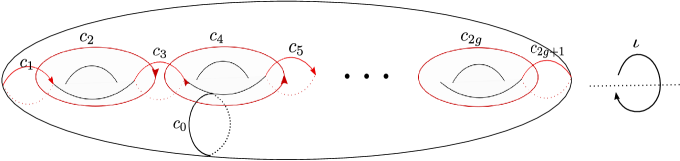
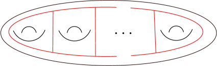
Let denote genus closed surface with no punctures, then is generated by the (left) Dehn twists around curves shown in Figure 1. There are relations among generators: the disjoint relation (far commutativity), the braid relations, the chain relation, the lantern relation and the hyperelliptic relation.
Definition 2.2.5 ([12]).
Let be the hyperelliptic involution in Figure 1 and let be the centralizer in of , i.e.,
The symmetric mapping class group, denoted by , is the group
Remark 2.2.6.
In general, a hyperelliptic involution is a order two mapping class acting on the homology by , and it is unique up to conjugations when genus [12, Proposition 7.15]. Here we pick the special as indicated in Figure 1.
Theorem 2.2.7 (Birman-Hilden Theorem).
For any , , where is the mapping class group of punctured sphere, or the spherical braid group . In particular, is generated by , they satisfy the relations in the braid group .
3. Hecke group inside mapping class group
3.1. Flat structure and Thurston’s construction
Definition 3.1.1.
A multicurve is a set of pairwise disjoint simple closed curves on the surface, the multitwist with multiplicity () about is a mapping class . For simplicity, we write .
Definition 3.1.2.
A pair of multicurves , bind the surface if they meet only at transverse double points, and every component of is a polygonal region with at least 4 sides (running alternately along and ).
Now view as a (bipartite) graph, where the vertexes are given by the simple closed curves in , and two vertexes are connected by edge iff the corresponding curves have geometric intersection number . We denote the graph by , and the corresponding adjacency matrix by , where . Let be a pair of multiplicities, we denote corresponding diagonal matrix by . If binds , then is connected, hence the matrix is primitive, and one can apply Perron–Frobenius theorem. We denote the Perron–Frobenius eigenvalue and eigenvector by , such that
| (3) | ||||
Given a surface , Thurston constructs a certain type of flat structure (singular Euclidean structure) on the surface [35], also see [42] for equivalent definitions of the flat structure. Here we will give one arising from polygons.
Definition 3.1.3 ([42]).
A flat structure on the surface is given by a cell decomposition consisting of a finite union of polygons in (Euclidean polygons), with a choice of pairing of parallel sides of equal length. Two sets of polygons are considered to define the same flat structure if one can be cut in to pieces along straight lines and these pieces can be translated and re-glued to form the other set of polygons.
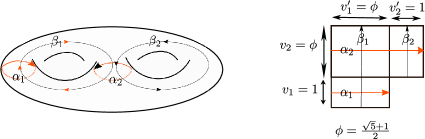
For example Figure 2 gives a flat structure on , where we have one vertex and it is the only 0-cell.
Now given a pair of multi curves binding , we construct a flat structure on which the corresponding multitwists act affinely.
We assign to be the length of curves in . Consider the dual cell decomposition of the obvious cell decomposition coming from cutting along the curves in (since binds ), the number of -cells is equal to the number of nonzero entries in , and each -cells is a rectangle. The length we assign to each -cell is equal to the length of the curve intersecting with it, see Figure 2. Using this flat stucture we get an action of a pair of multitwists with multiplicities.
Theorem 3.1.4 (Thurston’s construction [29, 35]).
Let , be a pair of multi curves binding the surface , and be a pair of multiplicities. Then we have a representation given by
Moreover, the map lifts to if and only if the curves in can be oriented so that their geometric and algebraic intersection numbers coincide .
Proof.
The curves in decompose the surface into copies of cylinders with height vector equal to , and circumference vector equal to . It is obvious one can make act affinely when restricted to each cylinder as indicated in Definition 2.2.2. Now from (3) the linear part of the action agrees on all cylinders. The same is true for . Therefore, the derivatives of and give the desired representation. When for , we have well defined horizontal and vertical directions, hence a linear representation. One can see [12, Chapter 14] or [29, Section 4] for more details. ∎
When , the corresponding graph and multiplicities are restrictive, one can see [16, Chapter 1.4] for the discussion on the graphs with norm less than . When there is no multiplicity, The graphs are of type or [22]. A little bit of calculations also show if there are multiplicities, then only type graph appears, with multiplicity two on a 1-valence vertex and the corresponding equals to the norm of the type Coxeter graph.
Remark 3.1.5.
Due to the Nielson-Thurston classification, a mapping class is either periodic, reducible or Pseudo-Anosov. Thurston used this construction to construct Pseudo-Anosov mapping class [35]. In fact, a mapping class in this construction is periodic, reducible or Pseudo-Anosov if and only if the image under is elliptic, parabolic or hyperbolic (determined by the traces).
The Riemann surfaces equipped with flat structures are called flat surfaces, which can also be described analytically by a pair , where is a closed Riemann surface, and is a holomorphic -form on . One can choose an atlas of such that has the form away from zeros for some charts with transition maps given by translations, and for the neighborhood of a zero has the form for some charts . There is natural action of , given by , where is the Riemann surface such that is holomorphic on . If we consider the flat surfaces in the sense of Definition 3.1.3, then the action is more explicit which is given by actions on polygons in . The study of the flat surfaces and their behaviors under the actions has wide applications in the study of geometry, topology and dynamic systems [43], In particular, by the results of Veech, ([37, 28]), the flat surface obtained by multicurves above has a nontrivial stablizer group which is a discrete subgroup of (or ) containing the group generated by affine automorphisms given by the multitwists.
3.2. Relation between two groups
Proposition 3.2.1.
[22] The representation is faithful when . When , the order of is at most .
Proof.
When , the image of is a free group on two generators The injectivitiy follows from the Hopfian property of the finite generated free group.
When with no multiplicities, see [22, Theorem 7.3], one has a homomorphism from to the automorphism group of the graph preserving the bicoloring, both the image and kernel are of order at most two and one of them is trivial. For the only case when it’s not multiplicity free, by Proposition 2.2.3 (b), the homomorphism has with trivial image, hence the proof is also valid. ∎
Proposition 3.2.2.
Let be the multi curves on as in Figure 1 with no multiplicities. We have
Proof.
It follows from next lemmas. ∎
Lemma 3.2.3.
Proof.
From direct computation only using braid group relations we have
The left hand side from the chain relation [12, Proposition 4.12] (it is not hard to get same relation for right Dehn twists), hence we get first equality.
Lemma 3.2.4.
Same setting as before, let , we have , where .
Proof.
By moving the elements with larger index to the left we can rewrite the product:
| (7) |
Now we prove the lemma by induction. When , the statement is obvious, suppose it’s true for , then when we have
∎
From Lemma 3.2.3 and 3.2.4, and the fact that commutes with all these Dehn twists, we have
| (8) |
Now from equation (8), , which has the order of at most (Proposition 3.2.1). Hence the Proposition 3.2.2 is proved.
Theorem 3.2.5.
Let , we have an injective homomorphism , by sending , , to , , respectively.
Proof.
The graph is of type with vertices, and it is not hard to orient curves so that their geometric and algebraic intersection numbers coincide as indicated in Figure 1 and Figure 2 (one may observe the difference coming from the parity of ). Therefore the map factors through . Now from Theorem 2.1.2, 3.1.4, Proposition 3.2.2 and the fact that , we have
∎
Corollary 3.2.6.
We have and .
3.3. Geometric discription of .
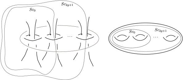
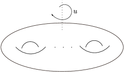
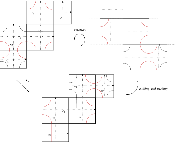
Now we give a geometric description of the element . Consider the heegaard splitting represented by Figure 3 , and denote the corresponding mapping class by , maps curves to for and the image of under is shown in the Figure 3. In fact, One can check direcly , which is a root of center in . We denote the horizontal rotation in Figure 4 by , It is clear .
Lemma 3.3.1.
in .
Proof.
Directly calculation shows , in fact we have [16]
Hence the corresponding flat structure has a rotation-by- symmetry. By the result of Veech [37] dicussed in previous subsection, or see [28, Section 5] and Theorem 3.2.5, is isotopic to the mapping class described in Figure 5 (here we give the proof for , but the proof works for any genus similarly). Then one can check geometricly how moves the set of simple closed curves for (Figure 1) and compare with the action of (It is clear how acts geometrically). If they agree on for all (regard as the isotopy class), then will fix all , hence, by Proposition 2.2.3 (b), commute with all the Dehn twists generating . The result for now follows from the fact that the center of is trivial when . When , the center is generated by the hyperelliptic involution , so it suffices to check their actions agrees on some curve with orientations. One can see the action on and are the only nonobvious cases to check. For other curves, they are parallel to the edges of the cell decomposition, hence easy to see two mapping classes agree on with orientations. We prove the case for and in Figure 5. We leave it to the reader to compare the curves in Figure 5 on the original surfaces. ∎
4. Topological quantum field theory
4.1. Notations
The standard references are [5, 6, 33], Let integer , . We denote the color set by . , when is even, and , when is odd. Let be a primitive -th root of unity when is even, and a primitive -th root of unity when is odd. For integer , let , where is the quantum integer, and . We also let , and . is the genus handlebody.
Definition 4.1.1.
Given a compact closed oriented three manifold, the skein space is the vector space spaned by all the isotopy classes of framed links in modulo Kaffuman bracket relations.
In particular, .
Given a framed link and an integer . One can color the curves using Jones-Wenzl idempotents () [18] [40]. Let denote the single curve winding once around the longitude, colored with -th Jones-Wenzl idempotent. Let . We use to denote the link obtained by replacing each components of by , and to denote the number we get by resolving the framed colored link in .
4.2. Invariants
Let be a three dimensional manifold obtained by doing surgery along a framed link in , we use to denote the Reshtikin-Turaev (RT) invariant of at level with a framed colored link , we have ( is the signature of the linking matrix of , and is the number of components of )
| (9) |
In particular, .
4.3. Vector space
The TQFT vector space of is constructed as the quotient of by the left kernel of any sesquilinear form induced by gluing of handlebodies [6, Prop. 1.9]. It is a finite dimensional vector space, and we will breifly recall the explicit basis constructed in [6], also see [23] for the pure skein construction.
Definition 4.3.1.
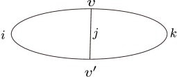
Given a trivalent vertex with edges colored by from the set . We say the vertex is admissible if the coloring satisfies:
Definition 4.3.2.
An admissible trivalent graph is an labeled trivalent graphs with all vertices admissible.
Definition 4.3.3.
Let be a (closed) surface bounding the handlebody and be a trivalent graph inside to which retracts. The TQFT vector space at level r is spanned by all the admissible trivalent graphs with being the underline graph, and all colors are from . Figure 6 shows one possible underline graph, admissibly coloring the graph produces one basis. We denote the basis vectors by , where is a function from the set of edges to . We also denote the handlebody with basis by , and we denote the TQFT vector space by . it corresponds to theory when is even, and theory when is odd.
Moreover we let , the dimension is given by the formula [6, Corollary 1.16]
| (10) |
One can relate different basis by doing -moves locally showing in Figure 7, where is the symbol , we also denote the tetrahedron coefficient by , one can find explicit formulas in, for example, [27].

For the more general setting one can see, for example [36], where TQFT is constructed from modular categories, the coloring corresponds to the simple objects in the category and the edges are morphisms. In the SU(2) and SO(3) case, the corresponding modular categories here are the TLJ-category (Temperle-Lieb-Jones category) [36, 39], simple objects here are Jones-Wenzl projections [18, 40], which have nice diagrammatic descriptions [39].
4.4. Projective action of mapping class group
Let , denote the corresponding mapping cylinder by , fix a basis for as in Definition 4.3.3, then we have a bilinear form given by . Where denotes with opposite orientation (hence the framing of curves inside will also be reversed). It is proven in [6] the bilinear form is nondegenrate (since the vector space is constructed by quotient out the kernel), and the form induced by identity mapping class is hermition, and the basis defined in Definition 4.3.3 forms an orthogonal basis. Moreover we have [6, Theorem 4.11]:
| (11) |
where given by evaluation of following diagram ( are colors of the edges intersecting at ).
In particular, let denote the basis vectors with zero coloring, one has
| (12) |
Now the linear action can be computed by the bilinear form: , and we have
| (13) |
The representation is projective since the signatures don’t behave well with respect to the gluing see, for example [36, Section IV] and [26, Lemma 2.8].
When we pick carefully, gives an inner product on . After some normalizations, our will be unitary, hence gives a unitary projective representation of
. We will simply use to denote .
It is in general very hard to compute directly, for example see [7] for the explicit formula for the set of Dehn twists generating the mapping class group, but for some special mapping class it is easy to write down the matrix.
When is the right (left) Dehn tiwst along a curve , then can be presented by surgery on the curve , which is framed relative to the surface (denoted by ). If bounds a disk in , for example curves , it is easy to resolve the diagrams and compute the invariant using Kirby calculus. One has
| (14) |
Where is the edge transverse to the disk bounded by .
When corresponds to a heeagard splitting of the , from the above discussion and the Formula (9), We have
Hence the entry of the can be computed by evaluating some tangle diagrams in , and this is how we compute . The diagram presentation for can be obtained easily from Lemma 3.3.1, see Figure 11 for the case when .


Now we will briefly describe two projective actions defined in [33], also see [26]. One is geometric, the other is skein theoretic, we denote them by and respectively. They give the same projective representation but slightly different central extensions [26], also see [15].
Fix a heegaard splitting of correspoding to some mapping class, for example the mapping class as defined in Theorem 3.2.5 (also see Lemma 3.3.1), we have , then can be viewd as the quotient of by the kernel of the form . There are natural left and right actions of on by pushing the curves in into and , and is itself an algebra. Moreover it is a -algebra, where the structure is induced by the map on . In particular it reverses framings relative to the surface, we use to denote the under the operation. We also denote the left action by , one has
| (15) |
Now since acts naturally on , it acts on . It is proved in [33] that is surjective, and moreover the kernel of is preserved by the action of . Therefore induces automorphisms of , it is inner since is finite dimensional. As a result, for any , there exists such that for any we have
| (16) |
Note is only well defined up to a constant, hence gives a projective representation. It is not hard to see satisfies (16) for any , indeed one observe
hence by (13), we have for any ,
| (17) | ||||
Now we will describe two actions.
Geometric action is defined on mapping classes which can be extended in or , we denote such mapping classes by respectively. Such mapping classes directly act on the diagrams inside handlebodies, we denote the action by . If , one define . If , define by
| (18) |
One can check the action satisfies (16) [33], and since generates , as a projective representation we have , and in particular, we have
| (19) |
for some nonzero constant (which depends on the choice of word representing ). Now for Dehn twists along curves which are in . They are diagonal matrix given by
| (20) |
For Dehn twists along curves which are in , see Figure 3 and Lemma 3.3.1. From (18), (20) and similar argument as in (17), we have for
| (21) |
Skein theoretic action is defined on the set of all the Dehn twists, denoted by , it is motivated by the surgery presentation of mapping cylinder corresponding to the Dehn twists as discussed above. Similarly, let be the right (left) Dehn tiwst along a curve , then the action is given by first cabling the curve by the skein element in , and then pushing it back in the handlebody , namely . Now if bounds a disk in , for example curves , we have similarly
| (22) |
If does not bound a disk, for example curves , one can make use of the Proposition 2.2.3 , so that can be map to the curves that bound a disk. For example the mapping class , we have for . Hence by (16), we have for ,
| (23) |
Compare equation (20) and (22), also from (23), we have as projective representations. In particular
| (24) |
for some nonzero constant (which depends on the choice of word representing ).
It is not hard to see and agrees on the word in and they are homomorphisms when restricted to or . Moreover they are unitary when the hermition form is positive definite.
Remark 4.4.1.
Lemma 4.4.2.
We have .
Proof.
Let be the -entry of the matrix . Since , and
it suffices to prove . We have
From Lemma 3.3.1, and the standard calculations using second identity in Figure 10, we have . It is nonzero if and only if . Therefore by (11), we have
where is the set of edges (in Figure 6) that invariant under the action of . Now consider unknots placed next to each other and all colored with , there are two ways to evaluate it. Direct evaluation gives , the other way is to apply the partition of identity (Figure 9) times, one gets a linear combination of . Resolving it using the second identity in Figure 10 as before, one get number . Therefore . ∎
Lemma 4.4.3.
Let be a word, be a word, and ( if is a word) is a word representing the mapping class , we have
| (25) |
where is the signature of link defined in [26, Sec. 2.3], and is the exponent sum of the word .
Proof.
We have
Proposition 4.4.4.
Let be the word , we have
| (26) |
Proof.
From Lemma 4.4.2, we have . Hence from (21) or (23), we have for ( agrees on those Dehn twists). Now since all the mapping classes related are in , they commute with . Moreover since , by similar but simpler argument as in Lemma 4.4.3, we have in particular commutes with and for . Therefore we have
Since (Corollary 3.2.6), the second equality follows from Lemma 4.4.2 and 4.4.3.
∎
Now we are ready for the main theorem.
Theorem 4.4.5.
We have projective (unitary) representations of from the TQFT vector spaces , and when the representations factor through . In particular. When , gives the modular data of TLJ modular categories, when , we have and a diagonal matrix , satisfying the relations:
| (27) | ||||
Proof.
Let and . From Lemma 4.4.2, Proposition 4.4.4 and Theorem 3.2.5, it gives a projective representation of . One can get a unitary representation by specializing to some appropriate root of unity, for example, . Normalizing the basis using (11), under normalized basis, and are unitary ([33]). In particular, up to a scalar, is unitary. Since its first row and column are all reals, same computation as in the proof of Lemma 4.4.2 shows that is indeed unitary.
For , it’s straight forward to see . The special cases in the theorem now follows from the computation of the signatures, when , , and when , .
∎
Remark 4.4.6.
In the remaining of this section, we will focus on the case when , and give concrete calculations. We denote the basis in by , which means the graph in Figure 6 is colored by from left to right, and we give them the dictionary order. Let , the matrix can be computed from evaluating following diagrams.
Therefore it is easy to see is a symmetric real matrix. And we have
| (28) | ||||
When the form is positive definite one can normalize the basis, we have a unitary matrix
| (29) |
is a diagonal matrix and the entries are all root of unities, hence always unitary.
Now we give formula to evaluate entries of
Proposition 4.4.7.
We have
| (30) |
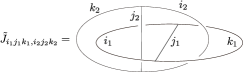
where is the coefficient of the following recoupling formula:
and
| (31) |
Proof.
Equation (31) follows from applying the identity on the left of Figure 10 and a F-move. Now one can resolve two double crossings in the diagram presentation of , and apply the identity on the right of Figure 10. The remaining diagram are two tetrahedrons connected along an edge, straight forward computations give us the Formula (30). ∎
Remark 4.4.8.
Now we give the calculation result for Ising theory and Fibonacci theory , which are done easily by hand and verified by using Maple software:
In particular, we have
Proposition 4.4.9.
The group is infinite.
Proof.
Since the projective factor is a root of unity, it suffices to work with . We compute the element . It has an eigenvalue , which is not a root of unity, since its minimal polynomial, , is not cyclotomic. ∎
Moreover since all the entries of matrices under unnormalized basis are in a cyclotomic field (only even powers of and appear when ), the Galois group naturally acts on the representations. In particular it preserves the property that the image is finite or not. Now let for odd , By computing the trace of the image of the Pseudo-Anosov mapping class , we have
and
Proposition 4.4.10.
The group is also infinite for .
Proof.
It suffices to check . Using Maple software we have following numerical results.
| 3 | 5 | 7 | 9 | 11 | 13 | |
| 5 | 14 | 30 | 55 | 91 | 140 | |
| 4.24 | 10.54 | 32.16 | 102.92 | 332.49 | 1084.12 |
We have when , which complete the proof. ∎
5. Spin structure and reducibility
The spin structure on a closed surface of genus is cohomology class which evaluates to one on the oriented fibre of the unit tangent bundle . In [17], Johnson built an one to one correspondence between the set of spin structures on a Riemann surface with the set of valued quadratic forms on with associated intersection form on (i.e. ). Moreover the bijection interwines the action of (induced by the obvious action of ), there are two orbits of the action depending on the parity of the spin structures, namely, the Arf invariant, which is an element in defined by
which is independent of the choice of symplectic basis for . The TQFT vector space , for , can be decomposed with respect to the spin structures on . Recall for the action of Dehn twist along a curve on the can be described by twisting the curve (make it -framed) in , attach a skein element and then push it back in the handlebody. Now we consider the curves in as the curves in , attached with the label , then there is a natural action by pushing it in the handlebody (). It is straight forward to show the action is in fact unitary [6, Prop 7.5]. Moreover the product induced by the algebra structure of gives the set of curves a structure of finite Heisenberg group (with the associated intersection form on ) [6]. Which is abelian and the characters are giving by valued quadratic forms on . Therefore one gets the decomposition
where each is the direct sum of the one dimensional representation associate with the quadratic form . Two orbits (parity) give two invariant subspace under action and the associate vector spaces for spin structures of same parity have same dimensions, which are denoted by respectively. We have , for . The formula for is given by [6, Thm 7.16]
| (32) |
Theorem 5.1.
when , the representation is reducible and has at least three irreducible summands.
Proof.
We choose oriented curves representing the standard symplectic basis. The spin structure associated with the flat structure can be describe by a quadratic form that assigns number (mod ) to (for ) [21, Section 3], where is the index of the curve . For example in Figure 5, we have for , and . Hence it is not hard to calculate its parity, which is equal to (mod ). Now the group generated by fix the flat structure, hence fix the associated spin structure, denoted by . We have following decomposition
from the dimension counting of the TQFT vector spaces associate to spin structures (32), when , dimensions for three summands are all nonzero.
∎
References
- [1] J. r. E. Andersen. Asymptotic faithfulness of the quantum representations of the mapping class groups. Ann. of Math. (2), 163(1):347–368, 2006.
- [2] J. r. E. Andersen, G. Masbaum, and K. Ueno. Topological quantum field theory and the Nielsen-Thurston classification of . Math. Proc. Cambridge Philos. Soc., 141(3):477–488, 2006.
- [3] G. Belletti, R. Detcherry, E. Kalfagianni, and T. Yang. Growth of quantum 6j-symbols and applications to the volume conjecture. arXiv:1807.03327v2, 2020.
- [4] J. S. Birman. Braids, links, and mapping class groups. Annals of Mathematics Studies, No. 82. Princeton University Press, Princeton, N.J.; University of Tokyo Press, Tokyo, 1974.
- [5] C. Blanchet, N. Habegger, G. Masbaum, and P. Vogel. Three-manifold invariants derived from the Kauffman bracket. Topology, 31(4):685–699, 1992.
- [6] C. Blanchet, N. Habegger, G. Masbaum, and P. Vogel. Topological quantum field theories derived from the Kauffman bracket. Topology, 34(4):883–927, 1995.
- [7] W. Bloomquist and Z. Wang. On topological quantum computing with mapping class group representations. J. Phys. A, 52(1):015301, 23, 2019.
- [8] P. Bruillard, S.-H. Ng, E. C. Rowell, and Z. Wang. On classification of modular categories by rank. Int. Math. Res. Not. IMRN, 2016(24):7546–7588, 2016.
- [9] A. Cappelli, C. Itzykson, and J.-B. Zuber. Modular invariant partition functions in two dimensions. Nuclear Phys. B, 280(3):445–465, 1987.
- [10] P. de la Harpe. Topics in geometric group theory. Chicago Lectures in Mathematics. University of Chicago Press, Chicago, IL, 2000.
- [11] R. Detcherry and E. Kalfagianni. Quantum representations and monodromies of fibered links. Adv. Math., 351:676–701, 2019.
- [12] B. Farb and D. Margalit. A primer on mapping class groups, volume 49 of Princeton Mathematical Series. Princeton University Press, Princeton, NJ, 2012.
- [13] M. H. Freedman, K. Walker, and Z. Wang. Quantum faithfully detects mapping class groups modulo center. Geom. Topol., 6:523–539, 2002.
- [14] L. Funar. On the TQFT representations of the mapping class groups. Pacific J. Math., 188(2):251–274, 1999.
- [15] P. M. Gilmer and G. Masbaum. Maslov index, lagrangians, mapping class groups and TQFT. Forum Math., 25(5):1067–1106, 2013.
- [16] F. M. Goodman, P. de la Harpe, and V. F. R. Jones. Coxeter graphs and towers of algebras, volume 14 of Mathematical Sciences Research Institute Publications. Springer-Verlag, New York, 1989.
- [17] D. Johnson. Spin structures and quadratic forms on surfaces. J. London Math. Soc. (2), 22(2):365–373, 1980.
- [18] V. F. R. Jones. Index for subfactors. Invent. Math., 72(1):1–25, 1983.
- [19] V. F. R. Jones. Hecke algebra representations of braid groups and link polynomials. Ann. of Math. (2), 126(2):335–388, 1987.
- [20] L. H. Kauffman and S. L. Lins. Temperley-Lieb recoupling theory and invariants of -manifolds, volume 134 of Annals of Mathematics Studies. Princeton University Press, Princeton, NJ, 1994.
- [21] M. Kontsevich and A. Zorich. Connected components of the moduli spaces of Abelian differentials with prescribed singularities. Invent. Math., 153(3):631–678, 2003.
- [22] C. J. Leininger. On groups generated by two positive multi-twists: Teichmüller curves and lehmer’s number. Geometry & Topology, 8(3):1301–1359, 2004.
- [23] W. B. R. Lickorish. Skeins and handlebodies. Pacific J. Math., 159(2):337–349, 1993.
- [24] Z. Liu and F. Xu. Jones-Wassermann subfactors for modular tensor categories. Adv. Math., 355:106775, 40, 2019.
- [25] G. Masbaum. An element of infinite order in TQFT-representations of mapping class groups. In Low-dimensional topology (Funchal, 1998), volume 233 of Contemp. Math., pages 137–139. Amer. Math. Soc., Providence, RI, 1999.
- [26] G. Masbaum and J. D. Roberts. On central extensions of mapping class groups. Math. Ann., 302(1):131–150, 1995.
- [27] G. Masbaum and P. Vogel. -valent graphs and the Kauffman bracket. Pacific J. Math., 164(2):361–381, 1994.
- [28] H. Masur and S. Tabachnikov. Rational billiards and flat structures. In Handbook of dynamical systems, Vol. 1A, pages 1015–1089. North-Holland, Amsterdam, 2002.
- [29] C. T. McMullen. Prym varieties and Teichmüller curves. Duke Math. J., 133(3):569–590, 2006.
- [30] M. Mignard and P. Schauenburg. Modular categories are not determined by their modular data. Lett. Math. Phys., 111(3):Paper No. 60, 9, 2021.
- [31] S.-H. Ng and P. Schauenburg. Congruence subgroups and generalized Frobenius-Schur indicators. Comm. Math. Phys., 300(1):1–46, 2010.
- [32] N. Reshetikhin and V. G. Turaev. Invariants of -manifolds via link polynomials and quantum groups. Invent. Math., 103(3):547–597, 1991.
- [33] J. Roberts. Skeins and mapping class groups. Math. Proc. Cambridge Philos. Soc., 115(1):53–77, 1994.
- [34] E. Rowell, R. Stong, and Z. Wang. On classification of modular tensor categories. Comm. Math. Phys., 292(2):343–389, 2009.
- [35] W. P. Thurston. On the geometry and dynamics of diffeomorphisms of surfaces. Bull. Amer. Math. Soc. (N.S.), 19(2):417–431, 1988.
- [36] V. G. Turaev. Quantum invariants of knots and 3-manifolds, volume 18 of De Gruyter Studies in Mathematics. Walter de Gruyter & Co., Berlin, revised edition, 2010.
- [37] W. A. Veech. Teichmüller curves in moduli space, Eisenstein series and an application to triangular billiards. Invent. Math., 97(3):553–583, 1989.
- [38] B. Wajnryb. A simple presentation for the mapping class group of an orientable surface. Israel J. Math., 45(2-3):157–174, 1983.
- [39] Z. Wang. Topological quantum computation, volume 112 of CBMS Regional Conference Series in Mathematics. Published for the Conference Board of the Mathematical Sciences, Washington, DC; by the American Mathematical Society, Providence, RI, 2010.
- [40] H. Wenzl. On sequences of projections. C. R. Math. Rep. Acad. Sci. Canada, 9(1):5–9, 1987.
- [41] E. Witten. Quantum field theory and the Jones polynomial. Comm. Math. Phys., 121(3):351–399, 1989.
- [42] A. Wright. Translation surfaces and their orbit closures: an introduction for a broad audience. EMS Surv. Math. Sci., 2(1):63–108, 2015.
- [43] A. Zorich. Flat surfaces. In Frontiers in number theory, physics, and geometry. I, pages 437–583. Springer, Berlin, 2006.