Shorter quantum circuits via single-qubit gate approximation

Abstract

We give a novel procedure for approximating general single-qubit unitaries from a finite universal gate set by reducing the problem to a novel magnitude approximation problem, achieving an immediate improvement in sequence length by a factor of 7/9. Extending the work of [Hastings2017, Campbell2017], we show that taking probabilistic mixtures of channels to solve fallback [BRS2015] and magnitude approximation problems saves factor of two in approximation costs. In particular, over the Clifford+$\sqrt{\textnormal{T}}$ gate set we achieve an average non-Clifford gate count of $0.23\log_{2}(1/\varepsilon)+2.13$ and T-count $0.56\log_{2}(1/\varepsilon)+5.3$ with mixed fallback approximations for diamond norm accuracy $\varepsilon$.

This paper provides a holistic overview of gate approximation, in addition to these new insights. We give an end-to-end procedure for gate approximation for general gate sets related to some quaternion algebras, providing pedagogical examples using common fault-tolerant gate sets (V, Clifford+T and Clifford+$\sqrt{\textnormal{T}}$). We also provide detailed numerical results for Clifford+T and Clifford+$\sqrt{\textnormal{T}}$ gate sets. In an effort to keep the paper self-contained, we include an overview of the relevant algorithms for integer point enumeration and relative norm equation solving. We provide a number of further applications of the magnitude approximation problems, as well as improved algorithms for exact synthesis, in the Appendices.

1 Introduction

In the quantum circuit model, quantum algorithms are expressed as sequences of unitary operations and measurements. Any $n$-qubit unitary can be implemented by a circuit of elementary gates, comprising controlled-NOT (CNOT) gates and single-qubit gates [Barenco1995]. Fault tolerant quantum computers require that the single-qubit gates belong to a finite set. Such a set is called universal if it generates a dense covering of $SU(2)$. That is, if any unitary $U\in SU(2)$ can be approximated to any accuracy by a finite sequence of gates from the set. Of particular interest is the subject of approximating single-qubit diagonal unitaries, as a Euler decomposition guarantees that any single-qubit unitary can be decomposed into diagonal $R_{z}$- and $R_{x}$-rotations. In addition, diagonal $R_{z}$ rotations are directly used in many quantum algorithm.

The cost of an approximation is quantified by the gate complexity, or gate cost. Associating each gate $g_{i}$ in a sequence with a weight $w_{i}$, the gate cost of that sequence is $\sum_{i}w_{i}$. The gate cost of approximating $U$ to within $\varepsilon$ is then taken as the minimum gate cost of all possible approximating sequences. Note that select gates, such as the Pauli or Clifford gates, are considered cheap to implement and so take zero weight. Typically, expensive gates will be given a weight of 1, so that the gate cost of an approximation corresponds to the number of expensive gates in the sequence. Consequently, minimizing the length of an approximating sequence is a problem integral to the subject of gate synthesis. A fundamental and general result is the Solovay-Kitaev theorem, which states that a universal gate-set $G$ can approximate any unitary $U\in SU(2)$ to accuracy $\varepsilon$ by a finite sequence of gates from $G$ of length $O(\log^{c}(1/\varepsilon))$, where $c$ is a constant. Significant progress has been made since Solovay-Kitaev for specific gate-sets associated with fault-tolerant quantum computers. Bourgain and Gamburd [bourgain2011spectral] showed that universal gate-sets of unitaries with algebraic entries give approximating sequences with lengths $O(\log(1/\varepsilon))$. Such gate-sets are called efficiently universal. This result was quickly applied to find efficient constructive algorithms for the Clifford$+$T gate set [A3, Selinger] and, later, the V basis [BGS]. Constructive algorithms for optimal diagonal approximations for both gate sets followed soon thereafter [RossSelinger2014, Ross2015, BlassEtAl2015]. Many of these algorithms adopted a common framework of integer point enumeration followed by a solving a norm equation.

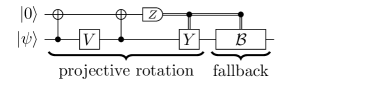
Figure 1: A fallback protocol circuit [BRS2015]. The circuit is composed of two steps, a projective rotation step and a fallback step. The projective rotation step effects one of two diagonal rotations on the input $\mathopen{}\left|\psi\right\rangle\mathclose{}$ depending on the $Z$-basis measurement outcome of the top ancilla qubit. The two rotation angles are determined by the matrix entries of the unitary $V$. If the measurement outcome is one, then a Pauli $Y$ is applied followed by the fallback step $\mathcal{B}$.

Measurements were also introduced to aid gate synthesis [paetznick2013repeat], culminating in the fall-back circuit (Figure 1), although this work was a departure from the common framework. Sarnak [sarnak2637letter] noted a connection between gate synthesis and quaternion algebras in his letter to Aaronson and Pollington, which has been used to build frameworks for both exact [Kliuchnikov2015a] and approximate synthesis [Kliuchnikov2015b]. The letter also characterizes ‘golden gate sets’, of which the Clifford$+$T and V gates are examples, that achieve optimal sequence lengths. For approximations of diagonal unitaries, this is shown to be $3\log_{\ell}(1/\varepsilon)$, where $\ell$ is a parameter determined by the number theoretic structure of each gate-set. These results are further expanded and generalizations of two-step approach to diagonal approximations from [RossSelinger2014] to other gate gets also discussed in [Parzanchevski]. Recent research [Campbell2017, Hastings2017] shows that approximation with quantum channels, rather than unitaries, achieves quadratic improvement in $\varepsilon$ and reduces the length by factor of two.

The quality of an approximation $V$ for some desired unitary $U$ is captured by the accuracy parameter $\varepsilon$. When we want to measure the distance between two unitary operators, we usually use the operator norm, which is the maximum singular value of the difference between the two operators. This allows us to bound how accurate a quantum algorithm is, based on how well we can approximate the unitary operations that make up the algorithm with other unitary operations [nielsen00]. However, in our work, we consider methods for approximating unitary operators using measurements, conditional gates, and probabilistic mixtures. This results in quantum channels, which are completely-positive trace-preserving linear maps on density matrices. To measure the distance between two $n$-qubit quantum channels, we use the diamond norm, which is defined as

$$\mathopen{}\left\|\mathcal{U}-\mathcal{V}\right\|\mathclose{}_{\diamond}=\max\limits_{\rho}\mathopen{}\left\{\mathopen{}\left\|((\mathcal{U}-\mathcal{V})\otimes\mathcal{I}_{2^{n}})\mathopen{}\left(\rho\right)\mathclose{}\right\|\mathclose{}_{1}\right\}\mathclose{},\text{ where }\mathopen{}\left\|A\right\|\mathclose{}_{1}=\mathrm{Tr}\sqrt{A^{\dagger}A}$$ (1)

where $\mathcal{I}_{2^{n}}$ is the identity map from $\mathbb{C}^{2^{n}\times 2^{n}}$ into $\mathbb{C}^{2^{n}\times 2^{n}}$ and the maximum is taken over all probability density matrices $\rho$. The diamond norm allows us to estimate the accuracy of a quantum algorithm based on the inaccuracies of the channels that make up the algorithm (Appendix LABEL:app:diamond-norm-properties). We also recall in Appendix LABEL:app:diamond-norm-properties that the diamond norm is bounded above by twice the spectral norm of the difference between the unitary operators that correspond to the channels. This makes it easy to compare our results, which are stated in terms of diamond norm accuracy, with previous results that are stated in terms of spectral norm accuracy.

We consider three universal gate sets associated with fault-tolerant quantum computation: the V basis, the Clifford+T basis and the Clifford+$\sqrt{\text{T}}$ basis. The Clifford+T gate set is commonly used for fault tolerant quantum computation, and is known to be efficiently universal [Selinger], with gate cost depending solely on the number of $T$ gates used. The V basis was shown to be efficiently universal in [harrow2002efficient], and provides a simple pedagogical example of approximation. The Clifford$+\sqrt{\text{T}}$ gate set is an alternative to the Clifford$+$T gate set for fault tolerant computing. The merits of these gate sets with regard to fault tolerant computing are discussed in greater detail in Section 1.1.

The rest of this paper is organized as follows. Section 2 summarizes our main results. In Section LABEL:sec:crypto-connection, we briefly discuss connections between gate synthesis and cryptography. Section 3 defines the five approximation problems that are the focus of this paper. We detail a complete method for solving these problems in Section 4, with examples for the V, Clifford$+$T and Clifford $+\sqrt{\text{T}}$ gate sets, in addition to a general solution. We provide extensive numerical results for our method in Section LABEL:sec:numerical-results for Clifford$+$T and Clifford$+\sqrt{\text{T}}$. Section LABEL:sec:point-enum and Section LABEL:sec:normeqsolv recall algorithms for solving two problems that arise in our solution method: integer point enumeration and norm equation solving.

1.1 Fault tolerant gate sets

Unitary synthesis translates the description of a quantum algorithm into a sequence of operations gates”) that can be implemented on the target quantum computer. The set of operations permitted by a particular quantum computing platform are limited by physical constraints and may not match the operations prescribed in the algorithm. Moreover, even if the operations offered by the quantum computer match the operations in the algorithm, the accuracy to which the quantum computer can perform each operation is likely to be limited. Loosely speaking, existing quantum computing systems offer single-qubit unitary operations with accuracy up to $10^{-4}$ (see Fig. S.17 in [Supremacy2019] for the accuracy of one and two qubit gates) whereas useful quantum algorithms require accuracy of $10^{-10}$ or better (see Table I in [Catalysis2021] for the typical number of gates in useful quantum algorithms).

Fault-tolerant quantum computation bridges the accuracy gap by encoding many physical qubits into a smaller number of logical qubits. To guarantee accuracy, logical qubits must be encoded at all times. Operations of the quantum algorithm must be performed on the logical qubits while they are encoded. Each logical operation must both preserve the code structure and carefully limit the spread of errors. Those requirements restrict the available set of logical quantum operations.

The cheapest form of logical operations involves executing the same physical operation to each of the physical qubits in the code. For example, some codes admit the logical Hadamard operation by executing the physical Hadamard operation to each physical qubit. Unfortunately, these so-called ”transversal” gates can yield only a sparse discrete set within a single quantum code [EastinKnill, BravyiKonig, WebsterBartlett].

Stabilizer codes, the most widely studied class of quantum error correcting codes, typically admit transversal implementation of some or all of the Clifford group—the group generated by {$H$, $S$, CNOT}. A broad and widely studied subset of stabilizer codes called CSS support transversal implementation of the CNOT operation, for example. Circuits composed of Clifford group operations have the added benefit of being efficiently simulable, an essential feature for the study of fault tolerant quantum computing schemes.

At least one operation outside of the Clifford group is required for universal quantum computation (see Theorem 6.7.3 in [Nebe2006]). In most fault-tolerant quantum computing proposals, that non-Clifford operation is the $T$ gate, $T=\left(\begin{smallmatrix}e^{-i\pi/8}&0\\ 0&e^{i\pi/8}\end{smallmatrix}\right)$. The logical $T$ operation is typically implemented by ”distillation” which combines many (noisy) physical $T$ gates with (less noisy) logical Clifford operations [BravyiKitaevDistillation]. Distillation is regarded as the most efficient known technique for non-Clifford gates, but remains roughly an order of magnitude more expensive than transversal operations despite much study [BeverlandDistillation]. Distillation can be used to construct other operations, but known distillation protocols are limited to operations that belong to the so-called ”Clifford hierarchy” introduced in [Gottesman1999]. Of the known distillation techniques the most cost competitive operations are $T$ and the three qubit double-controlled-Z (CCZ) [Gidney2019]. Controlled on the first two qubits, the CCZ gate sends $\mathopen{}\left|111\right\rangle\mathclose{}\rightarrow-\mathopen{}\left|111\right\rangle\mathclose{}$ and $\mathopen{}\left|x\right\rangle\mathclose{}\rightarrow\mathopen{}\left|x\right\rangle\mathclose{}$ for all other $x\in\{0,1\}^{3}$.

To the best of our knowledge, there are no operations outside of the Clifford hierarchy that admit implementation through distillation of the corresponding resource states. However, by including measurement it is possible to construct other kinds of circuits out of fault tolerant Clifford+$T$ gates. For example, $V_{Z}=(I+2iZ)/\sqrt{5}$ can be implemented with the circuit shown in Figure 2. The idea then is to approximate a unitary $U$ with a sequence of Clifford+$V_{Z}$ gates then substitute Figure 2 for each $V_{Z}$ in the sequence. Unfortunately, that strategy yields higher number of $T$ gates than synthesis with Clifford+$T$ alone. The strategy could be redeemed with cheaper Clifford+$T$ implementations of $V_{Z}$ or similar non-Clifford gates. But finding such circuits is difficult,and the best known circuits do not produce better resource requirements overall. Though we consider the $V$-basis gate set in this paper, it is largely for instructional purposes.

Incorporation of measurements into Clifford+$T$ circuits can be used to emulate other gates within the Clifford hierarchy, as well. For example, the gate $\sqrt{T}=\left(\begin{smallmatrix}e^{-i\pi/16}&0\\ 0&e^{i\pi/16}\end{smallmatrix}\right)$ can be implemented with Clifford+$T$ and measurements [LowerBounds2020]. Approximations with the set Clifford+$\sqrt{T}$, through emulation, use the the same number of $T$ gates as direct Clifford+$T$ sequences. Using Clifford+$\sqrt{T}$ gates, however, yields approximating sequences that are half the length of corresponding Clifford+$T$ sequences, offering an advantage when rotations must be executed as fast as possible.

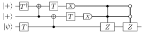
Figure 2: A Clifford+$T$ circuit implementation of $V_{Z}=(I+2iZ)/\sqrt{5}$ proposed in [paetznick2013repeat]. Conditioned on $X$-basis measurement outcomes of zero on the top two qubits, the circuit outputs $V_{Z}|\psi\rangle$. For any other measurement outcome the circuit outputs $|\psi\rangle$. Repeating the circuit until obtaining the 00 measurement outcome yields $V_{Z}|\psi\rangle$ using approximately $5.26$ $T$ gates, in expectation. The first conditional Pauli $Z$ gate is applied when measurement both outcomes are one, and the second conditional Pauli $Z$ gate is applied when both measurement outcomes are zero.

1.2 A roadmap to approximate quantum synthesis

Here we describe the standard approach to approximate unitary synthesis for a diagonal single-qubit unitary using the $V$ basis, then motivate generalisations to other gate sets and approximation techniques.

Suppose the approximation target is a single-qubit unitary $U\in SU(2)$, and target accuracy is some $\varepsilon>0$. The standard approach is to take the Euler decomposition of $U$, that is $U=e^{i\phi_{1}Z}e^{i\theta X}e^{i\phi_{2}Z}$ for real $\phi_{1},\theta,\phi_{2}$, and approximating each term independently. The matrices $e^{i\phi_{j}Z}$ are diagonal and we can diagonalize the central term by conjugation with Hadamard matrices. Now, for a diagonal target unitary, an approximation, $V=\left(\begin{smallmatrix}u&-v^{\ast}\\ v&u^{\ast}\end{smallmatrix}\right)$, is within $\varepsilon$ of the target if the top-left element resides within a pre-determined two-dimensional region. This region depends on the accuracy $\varepsilon$ and the rotation angle of the target unitary.

For approximation with the $V$ basis, unitaries that admit exact synthesis in $N$ gates are of the form $\frac{1}{\sqrt{5^{N}}}\left(\begin{smallmatrix}m_{1}&-m_{2}^{\ast}\\ m_{2}&m_{1}^{\ast}\end{smallmatrix}\right),$ where $m_{1}$ and $m_{2}$ are Gaussian integers, so in particular we have $m_{1}m_{1}^{*}+m_{2}m_{2}^{*}=5^{N}$. These matrices can additionally be efficiently factored into a sequence of basis elements. Moreover, given $N$ and $m_{1}$ there exists an efficient algorithm to determine whether an acceptable $m_{2}$ exists, and compute it if so. This establishes a general algorithm for approximate diagonal synthesis: repeatedly sample candidates for $m_{1}$ from a pre-determined approximation region and try to find a corresponding $m_{2}$, and when found apply the exact synthesis algorithm. Finding $m_{1}$ is a special case of integer point enumeration problem and finding $m_{2}$ is a special case of a relative norm equation problem, for both of which algorithms exist, discussed in Section LABEL:sec:point-enum and Section LABEL:sec:normeqsolv, respectively. A worked example of diagonal approximation with the $V$ basis is given in Section LABEL:sec:V-basis-example.

This three step process generalises quite well to other gate sets. A ‘good’ gate set generates unitaries of the form $\frac{1}{\sqrt{\ell^{N}}}\left(\begin{smallmatrix}m_{1}&-m_{2}^{\ast}\\ m_{2}&m_{1}^{\ast}\end{smallmatrix}\right)$, where $\ell$ is a parameter specific to the gate set and $N$ corresponds to the minimum number of basis gates required to synthesise that unitary. It is known [sarnak2637letter, KliuchnikovMaslovMosca2013, Kliuchnikov2015b] that the family of gate sets known as quaternion gate sets satisfy these conditions, and we rely on the framework of [KliuchnikovMaslovMosca2013, Kliuchnikov2015b] in particular to solve the relative norm equation to compute $m_{2}$ and for exact synthesis.

Further generalisations also exist. We find that established techniques of fallback approximation and probabilistic mixing align with the outlined approach, albeit leading to various other approximation regions. In Section 3 of this paper, we will additionally show that an alternative to the Euler decomposition method also follows the three steps, again with a modified approximation region, this time in one-dimension. In fact, modifying the approximation region is the only affect of these generalisations; the rest of the algorithm proceeds as before.

1.3 Paper outline

We summarize our main results in Section 2. Section 3 defines the five approximation problems that are the focus of this paper. We detail a complete method for solving these problems in Section 4, with examples for the V, Clifford$+$T and Clifford $+\sqrt{\text{T}}$ gate sets, in addition to a general solution. Section LABEL:sec:point-enum and Section LABEL:sec:normeqsolv recall algorithms for solving two problems that arise in our solution method: integer point enumeration and norm equation solving. Section LABEL:sec:exact-synthesis contains an algorithm for exact synthesis, which completes the gate approximation procedure. We provide extensive numerical results for the application of our method to single qubit gate approximation in Section LABEL:sec:numerical-results for Clifford$+$T and Clifford$+\sqrt{\text{T}}$, and outline further applications in Section LABEL:sec:magnitude-approx-applications. Finally, in Section LABEL:sec:crypto-connection, we discuss a number of related problems from other fields.

2 Summary of main results

Table 1: Scaling of the approximation cost for random angles. Approximation accuracy $\varepsilon$ is measured using diamond distance. Linear fit of the cost is based on the numerical results reported in Figure 3 and Figure LABEL:fig:clifford-root-t-random. Mixed diagonal rows contain results for our new and improved version of a mixed diagonal approximation protocol first introduced in [Campbell2017, Hastings2017]. Results from [Campbell2017, Hastings2017] apply to any gate set for which diagonal approximation is available, this is why we mark mixed diagonal results with New^∗. Fallback rows correspond to our improved and generalized fallback synthesis method (Figure 1) first introduced in [BRS2015]. For power cost, the cost of $T$ is two and the cost of $T^{1/2},T^{3/2}$ is three. Our algorithms are optimal with respect to this cost. For gate count cost, the cost of $T$, $T^{1/2},T^{3/2}$ is one. For $T$-count cost, the cost of $T$ is one and the cost of $T^{1/2},T^{3/2}$ is four. Clifford gate costs are always zero. Different costs are discussed in LABEL:sec:numerical-results. Heuristic cost estimates are discussed in LABEL:sec:cost-scaling. Applications of magnitude approximation are illustrated in Table 2.

Gate set	Approximation	Linear fit of the cost ($\varepsilon<10^{-4}$)		Heuristic	Novelty
(cost)	protocol	Mean	Max	cost estimate
	Diagonal [RossSelinger2014]	$3.02\log_{2}(1/\varepsilon)+1.77$	$3.02\log_{2}(1/\varepsilon)+9.19$	$3.0\log_{2}(1/\varepsilon)+O(1)$	Known
	Fallback [BRS2015]	$1.03\log_{2}(1/\varepsilon)+5.75$	$1.05\log_{2}(1/\varepsilon)+11.83$	$1.0\log_{2}(1/\varepsilon)+O(1)$	Improved
Clifford+$T$	Magnitude	–	–	$1.0\log_{2}(1/\varepsilon)+O(1)$	New
($T$-count)	Mixed diagonal	$1.52\log_{2}(1/\varepsilon)-0.01$	$1.54\log_{2}(1/\varepsilon)+6.85$	$1.5\log_{2}(1/\varepsilon)+O(1)$	Improved
Figure 3	Mixed fallback	$0.53\log_{2}(1/\varepsilon)+4.86$	$0.57\log_{2}(1/\varepsilon)+8.83$	$0.5\log_{2}(1/\varepsilon)+O(1)$	New
	Mixed magnitude	–	–	$0.5\log_{2}(1/\varepsilon)+O(1)$	New
	Diagonal	$3.02\log_{2}(1/\varepsilon)+2.80$	$3.01\log_{2}(1/\varepsilon)+8.53$	$3.0\log_{2}(1/\varepsilon)+O(1)$	New
	Fallback	$1.04\log_{2}(1/\varepsilon)+6.61$	$1.02\log_{2}(1/\varepsilon)+11.83$	$1.0\log_{2}(1/\varepsilon)+O(1)$	New
Clifford+$\sqrt{T}$	Magnitude	–	–	$1.0\log_{2}(1/\varepsilon)+O(1)$	New
(power)	Mixed diagonal	$1.53\log_{2}(1/\varepsilon)+1.06$	$1.58\log_{2}(1/\varepsilon)+4.98$	$1.5\log_{2}(1/\varepsilon)+O(1)$	New*
LABEL:fig:clifford-root-t-random-power	Mixed fallback	$0.56\log_{2}(1/\varepsilon)+5.32$	$0.62\log_{2}(1/\varepsilon)+7.66$	$0.5\log_{2}(1/\varepsilon)+O(1)$	New
	Mixed magnitude	–	–	$0.5\log_{2}(1/\varepsilon)+O(1)$	New
	Diagonal	$1.21\log_{2}(1/\varepsilon)+1.18$	$1.26\log_{2}(1/\varepsilon)+3.86$	$1.2\log_{2}(1/\varepsilon)+O(1)$	New
	Fallback	$0.42\log_{2}(1/\varepsilon)+2.68$	$0.44\log_{2}(1/\varepsilon)+5.13$	$0.4\log_{2}(1/\varepsilon)+O(1)$	New
Clifford+$\sqrt{T}$	Magnitude	–	–	$0.4\log_{2}(1/\varepsilon)+O(1)$	New
(gate count)	Mixed diagonal	$0.61\log_{2}(1/\varepsilon)+0.43$	$0.64\log_{2}(1/\varepsilon)+2.52$	$0.6\log_{2}(1/\varepsilon)+O(1)$	New*
LABEL:fig:clifford-root-t-random-rcount	Mixed fallback	$0.23\log_{2}(1/\varepsilon)+2.13$	$0.25\log_{2}(1/\varepsilon)+3.85$	$0.2\log_{2}(1/\varepsilon)+O(1)$	New
	Mixed magnitude	–	–	$0.2\log_{2}(1/\varepsilon)+O(1)$	New
	Diagonal	$3.03\log_{2}(1/\varepsilon)+2.48$	$3.25\log_{2}(1/\varepsilon)+14.40$	$3.0\log_{2}(1/\varepsilon)+O(1)$	New
	Fallback	$1.04\log_{2}(1/\varepsilon)+6.43$	$1.18\log_{2}(1/\varepsilon)+14.01$	$1.0\log_{2}(1/\varepsilon)+O(1)$	New
Clifford+$\sqrt{T}$	Magnitude	–	–	$1.0\log_{2}(1/\varepsilon)+O(1)$	New
($T$ count)	Mixed diagonal	$1.53\log_{2}(1/\varepsilon)+1.02$	$1.68\log_{2}(1/\varepsilon)+7.30$	$1.5\log_{2}(1/\varepsilon)+O(1)$	New*
LABEL:fig:clifford-root-t-random-tcount	Mixed fallback	$0.56\log_{2}(1/\varepsilon)+5.30$	$0.67\log_{2}(1/\varepsilon)+9.85$	$0.5\log_{2}(1/\varepsilon)+O(1)$	New
	Mixed magnitude	–	–	$0.5\log_{2}(1/\varepsilon)+O(1)$	New

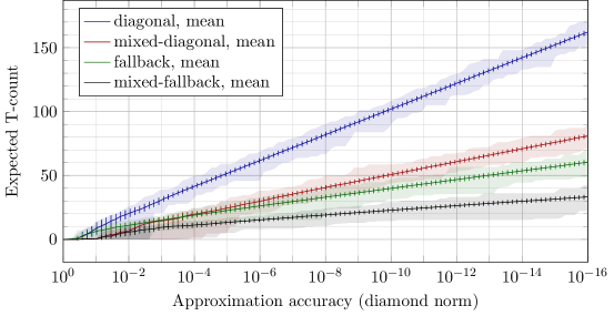
Figure 3: Cost of approximating a set of random diagonal rotation gates with Clifford+$T$ gates using four approximation protocols. Diagonal rotation angles are random angles drawn from the uniform distribution on $[0,2\pi]$. We fix a set of approximation accuracy values. For each value in the set we compute mean cost over all target angles. Vertical bars show the cost standard deviation for the given accuracy value. Shaded regions indicate range of costs from min to max over all angles for the given accuracy value. For the diagonal approximation protocol the cost for a given angle and given accuracy is equal to number of $T$ gates in the approximating sequence. For the other protocols the cost is the expectation of $T$-count. For example, if the first step of fall-back protocol requires 10 $T$ gates and fails with probability 0.01 and the step to correct failure requires 30 $T$ gates, the expected cost is 10.3. In all reported fallback protocols the probability of fallback is at most $0.01$.

Table 2: Examples of problems that benefit from magnitude approximation. The case of a general qubit unitary approximation is described in Section 3.1 and Section 3.6. Solutions to qubit approximation and general $\mathrm{SU}(4)$ approximation are outlined in LABEL:sec:magnitude-approx-applications. More generally, the magnitude approximation problem can be used when compiling $\mathrm{CNOT}$ and rotation circuits for isometries produced by UniversalQCompiler [Iten2016, Iten2021, Malvetti2021] for fault-tolerant quantum computers.

Problems that benefit from		Qubit state	General $\mathrm{SU}(2)$	General $\mathrm{SU}(4)$
magnitude approximation		preparation	approximation	approximation
	Number of real parameters	2	3	15
Problem	Number of magnitude	1	1	6
properties	approximation instances
	Number of diagonal	1	2	9
	approximation instances
Gate set	Approximation method	Heuristic T-count scaling with diamond norm accuracy $\varepsilon$
	Diagonal (known)	$6\log_{2}(1/\varepsilon)+O(1)$	$9\log_{2}(1/\varepsilon)+O(1)$	$45\log_{2}(1/\varepsilon)+O(1)$
Clifford+T	Diagonal + Magnitude (new)	$4\log_{2}(1/\varepsilon)+O(1)$	$7\log_{2}(1/\varepsilon)+O(1)$	$33\log_{2}(1/\varepsilon)+O(1)$
	Mixed Diagonal (improved)	$3\log_{2}(1/\varepsilon)+O(1)$	$4.5\log_{2}(1/\varepsilon)+O(1)$	$22.5\log_{2}(1/\varepsilon)+O(1)$
	Mixed Diag. + Mag. (new)	$2\log_{2}(1/\varepsilon)+O(1)$	$3.5\log_{2}(1/\varepsilon)+O(1)$	$11.5\log_{2}(1/\varepsilon)+O(1)$

In Section 3 we define six approximation problems: diagonal unitary approximation, fallback approximation, magnitude approximation and their versions with probabilistic mixing. The first two of these problems have been the subject of research for some time, with many results pertaining to specific gate sets [RossSelinger2014, KliuchnikovMaslovMosca2013, BGS, BRS2015, Kliuchnikov2015a, Kliuchnikov2015b]. The magnitude approximation problem is new and appears in our new approach to approximating an arbitrary unitary, $U$. When we independently approximate the three elements of the Euler angle decomposition of $U$, approximating the central term $e^{i\theta X}$ results in a unitary $V$ with entries of similar magnitude to the entries of $U$. Hence, the magnitude approximation problem. One of its applications is solving the general unitary approximation problem, which exploits the connection between unitary approximation and LPS graphs as we explain in Section LABEL:sec:crypto-connection. Explicitly, we adapt the path-finding algorithm of Carvalho Pinto and Petit [pinto2018better] to the quantum setting, requiring only two diagonal approximations and one more efficient magnitude approximation. The sequence costs obtained using our method improve on the standard Euler decomposition, which requires three diagonal approximations, by roughly one-third. More precisely, we find that the costs from magnitude approximation are one-third those of diagonal approximations. This means our approach to the general unitary approximation problem, which requires two diagonal approximations and one magnitude approximation, has a cost that is $7/9$ that of the standard Euler decomposition method.

Stier [stier] has concurrently and independently produced a similar result. We discuss additional applications of the magnitude approximation problem in LABEL:sec:magnitude-approx-applications.

The latter three problems are defined by applying the concept of channel mixing to diagonal, fallback and magnitude approximation, expanding on the ideas of [Campbell2017, Hastings2017]. Channel mixing employs a probabilistic combination of sequences of unitaries to approximate the target. The key idea is to use probabilistic combination of under-rotated and over-rotated approximations of a given target. We combine channel mixing with fallback and magnitude approximation to achieve a roughly two-fold improvement in cost compared to non-mixed problem variants.

To account for the fact that we are approximating with channels rather than unitaries, we use the diamond norm to measure the accuracy of approximation. We introduce the use of diagonal Clifford twirling, which ensures that the difference between the ideal and approximating channel is a Pauli channel. Because of this, we obtain a closed-form expression for the diamond distance which improves on analysis in [Campbell2017, Hastings2017] and results in lower approximation costs. The method in [Campbell2017] uses diagonal approximation algorithms as black-boxes and finds under-rotations and over-rotations by modifying target rotation angle. In contrast, we modify synthesis algorithms to directly find under and over-rotated approximations and further reduce approximations costs.

We provide a uniform approach to the six approximation problems and various gate sets. For each problem, we show that a constraint on the diamond norm can be reduced to a constraint on a single complex number. In contrast to [BRS2015], our approach to fallback approximation ensures desired success probability and approximation accuracy. The set of feasible solutions is represented geometrically as a region in $\mathbb{R}^{2}$, illustrated in Section 3. Figure 11 compares the areas of the regions associated to the approximation problems with respect to varying approximation accuracy $\varepsilon$ and success probability $q$. The scaling of the region area with epsilon determines the scaling of the approximation sequence cost with accuracy $\varepsilon$, as illustrated in Table 1. To establish dependence between region area scaling and cost scaling we use several heuristic assumptions as discussed in LABEL:sec:cost-scaling. We also provide experimental justification of relation between the cost and region scaling.

The results of our numerical experiments for Clifford+$T$ and Clifford+$\sqrt{T}$ gate sets are summarized in Table 1. More detailed numerical results for Clifford+$T$ are provided in Figure 3, in particular they show that linear fits for cost scaling with accuracy are well justified. Even more detailed results for Clifford+$T$ and for Clifford+$\sqrt{T}$ are in Section LABEL:sec:numerical-results. We show numerical results for approximating uniformly random diagonal rotations and angles and rotations by Fourier angles $\pi/2^{k}$. The study of uniformly random diagonal rotations is motivated by the use of diagonal rotations in quantum algorithm for chemistry, material science applications [TheoryOfTrotterError] and the rotations used in Quantum Signal Processing [QuantumSignalProcessing]; rotations by Fourier angles appear in the Quantum Fourier Transform [Nam2020] and preparation of Phase Gradient states [Gidney2018].

To provide practical context for our results, let us consider their impact on two practically interesting quantum dynamics and quantum chemistry problems, which are discussed in detail in Appendix F of [beverland2022assessing]. The quantum dynamics problem instance involves $30100$ diagonal rotation gates and requires an accuracy of $\varepsilon_{1}=1.1\cdot 10^{-8}$ per rotation. In this problem, rotations are the only non-Clifford gates used. The quantum chemistry instance involves $2.06\cdot 10^{8}$ diagonal rotations and requires an accuracy of $\varepsilon_{2}=1.6\cdot 10^{-11}$ per rotation. In addition to the diagonal rotation gates, this instance uses $5.4\cdot 10^{11}$ $T$ gates. To implement diagonal rotations with an accuracy of $\varepsilon_{1}$ using the mixed fallback protocol, we need an average of $20$ $T$ states, while for an accuracy of $\varepsilon_{2}$, we need an average of $26$ T states. When using Clifford+$\sqrt{T}$, the number of $T$, $\sqrt{T}$, and $\sqrt{T}^{3}$ gates in the approximating sequence is $8$ (on average) for $\varepsilon_{1}$ and $10$ (on average) for $\varepsilon_{2}$.

We find that Clifford+$\sqrt{T}$ is a promising gate-set for approximation when executing rotations as fast impossible. In this case the execution speed is limited by the gate count, in particular when executing rotations using a circuit from Figure 33 in [GameOfSurfaceCodes]. We achieve average gate-count scaling $0.23\log_{2}(1/\varepsilon)+2.13$ when using mixed fallback protocol with Clifford+$\sqrt{T}$ and T-count similar to Clifford+$T$ approximations. We assume that each $\sqrt{T}$ gate requires four $T$ gates, which is justified in LABEL:sec:cost-scaling. These are the first numerical studies of approximation cost scaling for Clifford+$\sqrt{T}$ gates that include additive constants, which are practically important because the $\log_{2}(1/\varepsilon)$ prefactor is small. These are also the first numerical results for mixed fallback and mixed diagonal approximations for Clifford+${T}$. We also provide more detail on approximate synthesis for general gate sets than the high-level approach outlined in [Parzanchevski].

In Section 4 we describe a complete method for solving the six approximation problems, restricting the scope to considering gate sets that can be represented by quaternion algebras. The general solution method is described in Section LABEL:sec:approximation-problems:general, and includes a process for constructing quaternion gate sets, as defined in [Kliuchnikov2015b]. To summarize, a gate set is defined by a complex field $L$, its maximal totally real subfield $K$ and a fixed set of elements in $K$. A solution to an approximation problem involves finding a matrix $M=\left(\begin{smallmatrix}m_{1}&-m_{2}^{\ast}\\ m_{2}&m_{1}^{\ast}\end{smallmatrix}\right)$ with entries in the integer ring of $L$. Our approach to finding $M$ can be summarized in two steps: point enumeration in a region defined by the approximation problem to find $m_{1}$, followed by solving a relative norm equation to recover $m_{2}$. To guide the reader, we work through three pedagogical examples: the V basis (Section 4.1), the Clifford$+$T basis (Section LABEL:sec:approximation-solutions-clifford-t), and the Clifford$+\sqrt{\textnormal{T}}$ basis (Section LABEL:sec:approximation-solutions-clifford-root-t).

3 Approximation problems

In this section we introduce six problems that address the approximation of qubit unitaries. Recall that in this paper we follow a two-step approach to solving approximation problems. First, in this section, we relate each problem to one-dimensional or two-dimensional regions, which define ‘good’ approximations. Second, in Section 4, we find sequences of gates $g_{1},\ldots,g_{n}$ over gate-set $G$ such that for a unitary computed by the sequence $g_{1}\ldots g_{n}=\mathopen{}\left(\begin{smallmatrix}u&-v^{\ast}\\ v&u^{\ast}\end{smallmatrix}\right)\mathclose{}$ the top-left entry $u$ belongs to a two-dimensional region of the complex plain, or the absolute values $|u|$ belongs to an interval, that is one-dimensional region. We show that this membership condition is sufficient for the unitary to be a good approximation. In this section we also show that these sequences $g_{1},\ldots,g_{n}$ then can be used to construct solutions to the approximation problems.

We begin by establishing some notation and key definitions [Kaye2007, nielsen00, watrous2018]. An arbitrary two-by-two unitary matrix with determinant one (i.e., a special unitary matrix) can be written as:

$$U=\mathopen{}\left(\begin{array}[]{cc}u&-v^{\ast}\\ v&u^{\ast}\end{array}\right)\mathclose{},\text{ for }u,v\in\mathbb{C}\text{ such that }\mathopen{}\left|u\right|\mathclose{}^{2}+\mathopen{}\left|v\right|\mathclose{}^{2}=1$$

Using the polar form of complex numbers we can write $u=r_{1}\exp\mathopen{}\left(i\psi_{1}\right)\mathclose{}$ and $v=ir_{2}\exp\mathopen{}\left(i\psi_{2}\right)\mathclose{}$. Let us introduce $r_{1}=\cos(\theta)$ and $r_{2}=\sin(\theta)$ for some $\theta\in[0,\pi/2]$ because $r_{1}^{2}+r_{2}^{2}=1$. The unitary $U$ can then be expressed as

$$U=\cos(\theta)e^{i\psi_{1}Z}+\sin(\theta)iXe^{i\psi_{2}Z}\text{ for }\psi_{1},\psi_{2},\theta\in\mathbb{R}$$ (2)

We will interchangeably use both parameterizations of a special unitary $U$. We denote the special unitary group, that is the group of all two by two unitary matrices with determinant equal to 1, by $\mathrm{SU}(2).$ We will also frequently use the fact that Pauli matrices are Hermitian and equal to their inverses.

A probabilistic ensemble of pure quantum states is represented as a trace-one positive semidefinite operator called a density matrix. The most general type of transformation on quantum state is a channel, a linear completely positive trace-preserving map on the space of density matrices. The action of a unitary $U$ on density matrix $\rho$ is given by

$$\mathcal{U}(\rho)=U\rho U^{\dagger}$$ (3)

and we refer to $\mathcal{U}$ as the “channel induced by $U$”. For diagonal unitaries of the form $e^{i\phi Z},e^{i\theta X}$ we denote the induced channel by

$$\mathcal{Z}_{\phi}(\rho)=e^{i\phi Z}\rho e^{-i\phi Z},\,\mathcal{X}_{\theta}(\rho)=e^{i\theta X}\rho e^{-i\theta X}$$ (4)

To measure the distance between channels we use the diamond norm

$$\mathopen{}\left\|\Phi\right\|\mathclose{}_{\diamond}:=\max_{\rho}\mathopen{}\left\|\left(\Phi\otimes\mathcal{I}\right)(\rho)\right\|\mathclose{}_{1}$$ (5)

where $\mathcal{I}$ is the channel induced by the identity matrix. For additional discussion and facts about the diamond norm see Appendix LABEL:app:diamond-norm-properties.

Our main goal in this paper is to solve single-qubit unitary approximation problems. The most general form is:

Problem 3.1 (General qubit unitary approximation).

Given:

• target unitary $U\in\mathrm{SU}(2)$,

• gate set $G$, a finite set of unitary matrices with determinant one

• accuracy $\varepsilon$, a positive real number

Find a channel $\mathcal{V}$ implemented using elements of $G$ and computational basis measurements such that

$$\mathopen{}\left\|\mathcal{U}-\mathcal{V}\right\|\mathclose{}_{\diamond}\leq\varepsilon,$$

where $\mathcal{U}$ is the channel induced by $U$.

In a simpler case, when channel $\mathcal{V}$ corresponds to unitary $V$ equal to the product $g_{1}\ldots g_{n}$ of two-by-two matrices from gate set $G$, the diamond norm is tightly bounded by twice the minimum spectral norm distance between $\pm U$ and $V$ (see LABEL:cor:diamond-distance-between-general). To avoid frequent explicit references to channels $\mathcal{U}$ and $\mathcal{V}$ induced by unitaries $U$ and $V$ we introduce distance between unitaries $U$ and $V$ as:

$$\mathcal{D}_{\diamond}\mathopen{}\left(U,V\right)\mathclose{}=\mathopen{}\left\|\mathcal{U}-\mathcal{V}\right\|\mathclose{}_{\diamond}.$$ (6)

Of particular interest is the case where $U$ is a diagonal unitary, namely $U=e^{i\phi Z}$ for real $\phi$. This case is very common in many quantum algorithms. In addition, the state-of-the-art way of solving the general unitary approximation problem is to use Euler angle decomposition to reduce the problem to three diagonal unitary approximation problems. Recall that $e^{i\theta X}=\cos\mathopen{}\left(\theta\right)\mathclose{}I+i\sin\mathopen{}\left(\theta\right)\mathclose{}X$. Euler decomposition is performed by solving for $\phi_{1},\phi_{2}$ in the equation below:

$$U=\cos(\theta)e^{i\psi_{1}Z}+\sin(\theta)iXe^{i\psi_{2}Z}=e^{i\phi_{1}Z}e^{i\theta X}e^{i\phi_{2}Z}={\cos\mathopen{}\left(\theta\right)\mathclose{}}e^{i\mathopen{}\left(\phi_{1}+\phi_{2}\right)\mathclose{}Z}+\sin\mathopen{}\left(\theta\right)\mathclose{}iXe^{i\mathopen{}\left(\phi_{2}-\phi_{1}\right)\mathclose{}Z}$$ (7)

To obtain the last equality we used the fact that $e^{i\phi Z}X=Xe^{-i\phi Z}$, since $XZX=-Z$ and for any invertible matrix $A$ and any matrix $B$, it is the case that $Ae^{B}A^{-1}=e^{ABA^{-1}}$.

In this section, we demonstrate how the general unitary approximation problem reduces to two diagonal approximations and a search for elements in a one-dimensional (1D) region, that we call magnitude approximation problem, improving on the traditional Euler angle decomposition approach. We then introduce a series of four problems for approximating diagonal unitaries, corresponding to the combinations of using probabilistic mixing (or not) and using fallback protocols [RUS1] (or not). For each problem we give a reduction to the search for elements in two-dimensional (2D) regions. We conclude the section with applying mixing to the magnitude approximation. Table 3 summarizes this section.

Table 3: Summary of the qubit unitary approximation protocols. Each protocol corresponds to a ”key problem” for which the top-left entry of matrix $\mathopen{}\left(\begin{smallmatrix}u&-v^{\ast}\\ v&u^{\ast}\end{smallmatrix}\right)\mathclose{}$ belongs to a two-dimensional region of complex plain, or the absolute value $|u|$ belongs to a one-dimensional interval. Some approximation protocols use others as sub-protocols. Combining the solution to the key problem(s) with the sub-protocols is described by the statements in ”Full protocol analysis” column. Comparisons of the geometric regions are given in Section 3.7, Table 4 and Figure 10. For cost scaling see Table 1 and Table 2.

Approximation		Target	Key	Key	Full	Sub-
protocol	Section	unitary	problem	problem	protocol	protocols
			definition	region	analysis
General	Section 3.1	$\mathrm{SU}(2)$	3.2	3.2	3.4	Diagonal or
unitary			(magnitude)	Figure 4		Fallback
Mixed general	Section 3.6	$\mathrm{SU}(2)$	3.19	3.21	3.22	Mixed diagonal
unitary			(magnitude)	Figure 9		or mixed fallback
Diagonal	Section 3.2	$e^{i\varphi Z}$	3.5	3.7	3.7	-
unitary			(diagonal)	Figure 5
Mixed	Section 3.4	$e^{i\varphi Z}$	3.11	3.13	3.13	-
diagonal unitary			(diagonal)	Figure 7
Fallback	Section 3.3	$e^{i\varphi Z}$	3.8	3.9	3.10	Diagonal
(Figure 1)			(projective)	Figure 6
Mixed	Section 3.5	$e^{i\varphi Z}$	3.16	3.18	3.17	Mixed diagonal
fallback			(projective)	Figure 8

3.1 Magnitude approximation

In the general unitary approximation problem (Problem 3.1), the task is to approximate an arbitrary unitary $U$. The standard approximation strategy is to use the Euler angle decomposition $U=e^{i\phi_{1}Z}e^{i\theta X}e^{i\phi_{2}Z}$ and independently approximate the three elements of the product. Our new approach is to first approximate $e^{i\theta X}$ up to phases, that is finding a unitary $V$ equal to $e^{i\phi^{\prime}_{1}Z}e^{i\theta^{\prime}X}e^{i\phi^{\prime}_{2}Z}$ such that $\theta$ and $\theta^{\prime}$ are close. In other words only magnitudes of entries of $U$ and $V$ are close, and phases $\phi^{\prime}_{1}$ and $\phi^{\prime}_{2}$ are arbitrary. We then re-express $U$ as:

$$U=e^{i(\phi_{1}-\phi^{\prime}_{1})Z}\underline{e^{i\phi^{\prime}_{1}Z}e^{i\theta X}e^{i\phi^{\prime}_{2}Z}}e^{i(\phi_{2}-\phi^{\prime}_{2})Z}.$$ (8)

The underlined middle part of the product is approximated by $V$, so it remains to approximate two diagonal $Z$ rotations.

The first main insight behind this strategy is that magnitude approximations have lower cost (see Table 1 and LABEL:sec:cost-scaling) and are easier to find than diagonal approximations. The second insight is that, for a random angle $\theta$, the approximation cost of a diagonal unitary $e^{i\theta Z}$ is independent of $\theta$ (see Figure 3 and LABEL:sec:numerical-results). Therefore, we may freely adjust the angles of the $Z$-axis rotations in the Euler decomposition in order to compensate for phase inaccuracy of the $X$-axis rotation. This results in a circuit that is approximately $7/9$ times the length, in terms of gate-count, of the solution resulting directly from Euler decomposition. An analogous strategy, discussed in Section LABEL:sec:crypto-connection, was developed by Carvalho Pinto and Petit in [pinto2018better] for path finding in LPS graphs, and they noted that their method could be adapted to the quantum setting. This was also confirmed by Stier [stier], concurrent to the work done in this paper. To construct $V$, we use the following proposition, which determines the approximate synthesis of any unitary by imposing the condition that the norm of its upper left element lies in a given interval.

Proposition 3.2 (Magnitude approximation condition).

Let $\theta$ be from $[0,\pi/2]$ and $\varepsilon\leq 2$ be a positive real number. Suppose that we have found a special unitary $V$

$$V=g_{1}\ldots g_{n}=\mathopen{}\left(\begin{array}[]{cc}u&-v^{\ast}\\ v&u^{\ast}\end{array}\right)\mathclose{}$$

over gate set $G$ such that $|u|$ belongs to the interval $\left\{\cos(\theta^{\prime\prime}):\theta^{\prime\prime}\in[0,\pi/2],|\theta^{\prime\prime}-\theta|\leq\delta\right\}$ for $\delta=\arcsin(\varepsilon/2)$.

Then unitary $V$ satisfies the inequality $\mathcal{D}_{\diamond}\mathopen{}\left(V,e^{i\phi_{1}^{\prime}Z}\underline{e^{i\theta X}}e^{i\phi_{1}^{\prime}Z}\right)\mathclose{}\leq\varepsilon$, for $\phi_{1}^{\prime}$ and $\phi^{\prime}_{2}$ defined by the equality $V=e^{i\phi_{1}^{\prime}Z}e^{i\theta^{\prime}X}e^{i\phi_{1}^{\prime}Z}$ with $\theta^{\prime}\in[0,\pi/2]$. We call such $V$ a magnitude $\varepsilon$-approximation of $e^{i\theta X}$. For a geometric interpretation of the constraint see Figure 4.

Proof.

By unitary invariance property of the diamond norm (see LABEL:prop:diamond-norm-unitary-invariance), distance $\mathcal{D}_{\diamond}\mathopen{}\left(V,e^{i\phi_{1}^{\prime}Z}\underline{e^{i\theta X}}e^{i\phi_{1}^{\prime}Z}\right)\mathclose{}$ is equal to $\mathcal{D}_{\diamond}\mathopen{}\left(e^{i\theta^{\prime}X},e^{i\theta X}\right)\mathclose{}$. Now we use the the fact that diamond norm distance between unitaries $U$ and $V$ is equal to the diameter of the smallest disc containing eigenvalues of $U^{\dagger}V$ (see LABEL:thm:diamond-distance-between-unitary-channels). The eigenvalues of $e^{i(\theta^{\prime}-\theta)X}$ are $e^{\pm i(\theta-\theta^{\prime})}$ because Hadamard diagonalizes $e^{i\phi X}=He^{i\phi Z}H$. Because we only have two eigenvalues, the diameter of the disc containing them is equal to distance $|e^{i(\theta-\theta^{\prime})}-e^{-i(\theta-\theta^{\prime})}|$, which is equal to $2|\sin(\theta-\theta^{\prime})|$. It remain to upper-bound this quantity. By definition of $\theta^{\prime}$, $|u|=\cos\mathopen{}\left(\theta^{\prime}\right)\mathclose{}$. This implies that $|\theta^{\prime}-\theta|\leq\delta$ because cosine is a bijection from $[0,\pi/2]$ onto $[0,1]$. Using $\sin(\delta)=\varepsilon/2$ we get the required bound. ∎

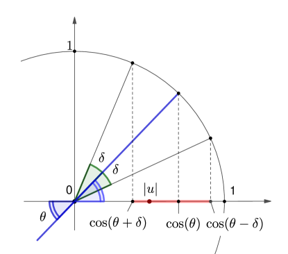
Figure 4: Geometric interpretation of the constraint on complex number $u$ appearing in Proposition 3.2. Possible absolute values $|u|$ belong to the interval $\left\{\cos(\theta^{\prime\prime}):\theta^{\prime\prime}\in[0,\pi/2],|\theta^{\prime\prime}-\theta|\leq\delta\right\}$ for $\delta=\arcsin(\varepsilon/2)$ and are shown as blue and dashed blue segments on the horizontal axis.

Note that when $\arcsin(\varepsilon/2)\leq\theta\leq\pi/2-\arcsin(\varepsilon/2)$, the absolute value $|u|$ must simply belong to interval $[{\cos(\theta-\arcsin(\varepsilon/2))},\cos(\theta+\arcsin(\varepsilon/2))]$.

Remark 3.3.

Since in practice $\varepsilon$ is chosen to be very small, we are able to take the approximation $\arcsin(x)\approx x$ in Proposition 3.2, hence, $\delta\approx\varepsilon/2$.

A simple way to leverage Proposition 3.2 for general unitary approximation is to split the accuracy $\varepsilon$ evenly among the three factors of the Euler decomposition. Then, use Proposition 3.2 to find a magnitude $\epsilon/3$-approximation of the $X$-axis rotation. Finally, find $\varepsilon/3$-approximations of the two remaining $Z$-axis rotations, adjusting the angles to compensate for the phase inaccuracy of the $X$-axis rotation. This strategy is captured formally in the following proposition.

Proposition 3.4 (General unitary approximation).

Suppose we are given a target unitary $U=e^{i\phi_{1}Z}e^{i\theta X}e^{i\phi_{2}Z}$ and target accuracy $\varepsilon$. Let $V$ be a magnitude $\varepsilon_{0}$-approximation of $e^{i\theta X}$ (see 3.2) and let $V=e^{i\phi^{\prime}_{1}Z}e^{i\theta^{\prime}X}e^{i\phi^{\prime}_{2}Z}$. Let channels $\Psi_{k}$ be within diamond norm distance $\varepsilon_{k}$ from unitary $e^{i(\phi_{k}-\phi^{\prime}_{k})Z}$, for $k=1,2$, and let $\varepsilon\geq\varepsilon_{0}+\varepsilon_{1}+\varepsilon_{2}$.

Then channel $\mathcal{U}$ induced by $U$ and composition $\Psi_{1}\mathcal{V}\Psi_{2}$ satisfy

$$\mathopen{}\left\|\mathcal{U}-\Psi_{1}\mathcal{V}\Psi_{2}\right\|\mathclose{}_{\diamond}\leq\varepsilon\text{, where }\mathcal{V}\text{ is the channel induced by }V.$$

Proof.

Let us write $U$ as a product $U_{1}U_{0}U_{2}$, where $U_{k}=e^{i(\phi_{k}-\phi^{\prime}_{k})Z}$ and $U_{0}=e^{i\phi^{\prime}_{1}Z}e^{i\theta X}e^{i\phi^{\prime}_{2}Z}$. We then write channel $\mathcal{U}$ as composition of channels $\mathcal{U}_{1}\mathcal{U}_{0}\mathcal{U}_{2}$, where $\mathcal{U}_{k}$ is the channel induced by $U_{k}$. Using the chain rule for diamond norm we have:

$$\mathopen{}\left\|\mathcal{U}-\Psi_{1}\mathcal{V}\Psi_{2}\right\|\mathclose{}_{\diamond}=\mathopen{}\left\|\mathcal{U}_{1}\mathcal{U}_{0}\mathcal{U}_{2}-\Psi_{1}\mathcal{V}\Psi_{2}\right\|\mathclose{}_{\diamond}\leq\mathopen{}\left\|\mathcal{U}_{1}-\Psi_{1}\right\|\mathclose{}_{\diamond}+\mathopen{}\left\|\mathcal{U}_{0}-\mathcal{V}\right\|\mathclose{}_{\diamond}+\mathopen{}\left\|\mathcal{U}_{2}-\Psi_{2}\right\|\mathclose{}_{\diamond}$$ (9)

By 3.2 $\mathopen{}\left\|\mathcal{U}_{0}-\mathcal{V}\right\|\mathclose{}_{\diamond}\leq\varepsilon_{0}$. Combining this bound with Equation 9 completes the proof. ∎

One can optimize the choices of $\varepsilon_{k}$ in the above 3.4. For random diagonal approximation, the cost scales as $3\log_{2}(1/\varepsilon)+O(1)$ and for random magnitude approximation the cost scales as $\log_{2}(1/\varepsilon)+O(1)$ (see Table 1). To minimize overall sequence length one can choose $\varepsilon_{1}=\varepsilon_{2}=0.43\varepsilon$ and $\varepsilon_{0}=0.14\varepsilon$, however this improves the sequence length only by a small additive constant $0.95$ in comparison to distributing errors equally.

3.2 Diagonal unitary approximation

The Euler angle decomposition Equation 7 describes a qubit unitary as a product of two diagonal unitaries of the form $e^{i\theta Z}$ and one $X$ rotation of the form $e^{i\theta X}$. Proposition 3.2 further reduces the $X$ rotation to a one-dimensional search problem, leaving just the diagonal unitaries. Therefore, the special case of diagonal unitary approximation is relevant to the general unitary approximation problem. In this section we recall some of the known results regarding the diagonal approximation problem.

Problem 3.5 (Diagonal unitary approximation).

Given:

• target angle $\theta$, a real number,

• gate set $G$, a finite set of two by two unitary matrices with determinant one,

• accuracy $\varepsilon$, a positive real number,

Find a sequence $g_{1},\ldots,g_{n}$ of elements of $G$ such that

$$\mathcal{D}_{\diamond}\left(\exp(i\theta Z),g_{1}\dots g_{n}\right)\leq\varepsilon.$$

Observe that Problem 3.5 is a special case of the general unitary approximation problem, where the target unitary is diagonal and approximating channel $\mathcal{V}$ is induced by unitary $g_{1}\dots g_{n}$. The diagonal unitary approximation problem is easier to solve because it admits the following bound on the diamond norm that depends only on the top left entry of $V=g_{1}\ldots g_{n}.$

Lemma 3.6 (Diamond difference from a diagonal unitary).

Given an angle $\theta$ and a unitary

$$V=\mathopen{}\left(\begin{array}[]{cc}u&-v^{\ast}\\ v&u^{\ast}\end{array}\right)\mathclose{},$$

the distance

$$\mathcal{D}_{\diamond}(e^{i\theta Z},V)=2\sqrt{1-\left(\mathrm{Re}(ue^{-i{\theta}})\right)^{2}}\leq 2\sqrt{2-2|\mathrm{Re}\mathopen{}\left(ue^{-i\theta}\right)\mathclose{}|}.$$

Proof of this bound is in LABEL:cor:diamond-distance-between-general-and-diaognal in Appendix LABEL:app:diamond-norm-properties. Lemma 3.6 immediately suggests a simple condition for solutions of the diagonal approximation problem.

Proposition 3.7 (Diagonal approximation condition).

Let $g_{1},\dots,g_{n}$ be a sequence of gates from a gate set $G$ and let

$$g_{1}\dots g_{n}=\mathopen{}\left(\begin{array}[]{cc}u&-v^{\ast}\\ v&u^{\ast}\end{array}\right)\mathclose{}.$$

Then $g_{1},\dots,g_{n}$ is a solution to the diagonal approximation problem for target angle $\theta$, gate set $G$ and accuracy $\varepsilon$ if

$$\mathopen{}\left|\mathrm{Re}\left(ue^{-i\theta}\right)\right|\mathclose{}\geq\sqrt{1-\varepsilon^{2}/4}.$$ (10)

For a geometric interpretation of the constraints see Figure 5.

Proof.

Let $\mathcal{V}$ be the channel induced by unitary $V=g_{1}\dots g_{n}$. Then by Lemma 3.6

$$\mathopen{}\left\|\mathcal{Z}_{\theta}-\mathcal{V}\right\|\mathclose{}_{\diamond}=2\sqrt{1-|\mathrm{Re}(ue^{-i\theta})|^{2}}\leq 2\sqrt{\varepsilon^{2}/4}=\varepsilon.$$ (11)

∎

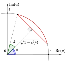
Figure 5: Geometric interpretation of constraints on complex number $u$ appearing in  Proposition 3.7. The region with red boundary contains complex numbers $u$ that satisfy constraints $\mathrm{Re}\mathopen{}\left(ue^{-i\theta}\right)\mathclose{}\geq\sqrt{1-\varepsilon^{2}/4}$ and $\mathopen{}\left|u\right|\mathclose{}\leq 1$. Note that the segment spans points with angular coordinates $[\theta-\delta,\theta+\delta]$ for $\delta=\arcsin(\varepsilon/2)$. Constraints in Proposition 3.7 lead to two regions: one with segment spanning points with angular coordinates $[\theta-\delta,\theta+\delta]$ and another one with $[\pi+\theta-\delta,\pi+\theta+\delta]$.

3.3 Fallback approximation

Fallback protocols [BRS2015] offer a more efficient way to approximate diagonal unitaries by incorporating measurements. A fallback protocol is a non-deterministic single-qubit quantum channel consisting of two steps: a projective rotation and a conditional fallback. The projective rotation and fallback steps may be implemented in a variety of ways. We limit our discussion to fallback protocols with the form illustrated in Figure 1.

For a fixed single-qubit unitary

$$V=\left(\begin{array}[]{cc}u&-v^{\ast}\\ v&u^{\ast}\end{array}\right)$$ (12)

the corresponding projective rotation effects one of two diagonal rotations on $\mathopen{}\left|\psi\right\rangle\mathclose{}$ depending on the measurement outcome. With probability $|u|^{2}$ the measurement outcome is zero, the projective rotation is said to have “succeeded” and the input state undergoes the transformation

$$\mathopen{}\left|\psi\right\rangle\mathclose{}\mapsto e^{i\theta_{0}Z}\mathopen{}\left|\psi\right\rangle\mathclose{}=e^{i\mathrm{Arg}(u)Z}\mathopen{}\left|\psi\right\rangle\mathclose{}.$$ (13)

otherwise, the measurement outcome is one, the projective rotation is said to have “failed” and

$$\mathopen{}\left|\psi\right\rangle\mathclose{}\mapsto e^{i\theta_{1}Z}\mathopen{}\left|\psi\right\rangle\mathclose{}=e^{i\mathrm{Arg}(v)Z}\mathopen{}\left|\psi\right\rangle\mathclose{}.$$ (14)

The projective rotation is intended to approximate a target diagonal unitary $e^{i\theta Z}$ so that $\theta_{0}\approx\theta$. The constraints necessary to achieve that goal are captured by the following problem.

Problem 3.8 (Projective approximation).

Given:

• target angle $\theta$, a real number,

• success probability $q$, a positive real number between $0$ and $1$,

• gate set $G$, a finite set of two by two unitary matrices with determinant one,

• accuracy $\varepsilon$, a positive real number,

find a sequence $g_{1},\ldots,g_{n}$ of elements in $G$, such that for $u,v$ defined via $g_{1}\ldots g_{n}=\left(\begin{array}[]{cc}u&-v^{\ast}\\ v&u^{\ast}\end{array}\right)$ the following holds:

• $|u|^{2}\geq q$, and

• $\mathcal{D}_{\diamond}\left(e^{i\theta Z},e^{i\mathrm{Arg}(u)Z}\right)\leq\varepsilon$.

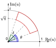
Figure 6: Geometric interpretation of constraint on complex number $u$ appearing in Proposition 3.9. The region with red boundary contains complex numbers $u$ that satisfy constraints $\mathrm{Arg}\mathopen{}\left(u\right)\mathclose{}\in[\theta-\delta,\theta+\delta]$ and $\mathopen{}\left|u\right|\mathclose{}\geq q$, where $\delta=\arcsin(\varepsilon/2)$. Constraints in Proposition 3.9 lead to two regions: one with $\mathrm{Arg}\mathopen{}\left(u\right)\mathclose{}\in[\theta-\delta,\theta+\delta]$ and another one with $\mathrm{Arg}\mathopen{}\left(u\right)\mathclose{}\in[\pi+\theta-\delta,\pi+\theta+\delta]$

Much like the case of the diagonal approximation problem (3.5), solutions to Problem 3.8 can be characterized entirely by conditions on the complex value $u$ at the top-left entry of the circuit unitary $g_{1}\ldots g_{n}$. These conditions are, however, less restrictive than those prescribed by Proposition 3.7. We compare the conditions in detail in Section 3.7 with the geometric representations shown in Figure 10.

Proposition 3.9 (Projective approximation condition).

Let $g_{1},\dots,g_{n}$ be a sequence of gates from a gate set $G$ and $g_{1}\ldots g_{n}=\mathopen{}\left(\begin{smallmatrix}u&-v^{\ast}\\ v&u^{\ast}\end{smallmatrix}\right)\mathclose{}$. Then $g_{1},\dots,g_{n}$ is a solution to the projective approximation problem (Problem 3.8) if $u$ satisfies

$$\mathopen{}\left|u\right|\mathclose{}\geq\sqrt{q}\mathrm{\leavevmode\nobreak\ and\leavevmode\nobreak\ }\left(\sin\mathopen{}\left|\mathrm{Arg}(u)-\theta\right|\mathclose{}\leq\varepsilon/2\mathrm{\leavevmode\nobreak\ or\leavevmode\nobreak\ }\sin\mathopen{}\left|\mathrm{Arg}(u)-(\theta+\pi)\right|\mathclose{}\leq\varepsilon/2\right)$$

For a geometric interpretation of these constraints see Figure 6.

Proof.

The condition $|u|\geq\sqrt{q}$ is equivalent to $|u|^{2}\geq q$ from Problem 3.8.

It remains to show that $\mathopen{}\left\|\mathcal{Z}_{\theta}-\mathcal{Z}_{\mathrm{Arg}(u)}\right\|\mathclose{}_{\diamond}\leq\varepsilon$. According to LABEL:cor:diamond-distance-between-diaognal, we have $\mathopen{}\left\|\mathcal{Z}_{\theta}-\mathcal{Z}_{\mathrm{Arg}(u)}\right\|\mathclose{}_{\diamond}\leq 2\sin|\mathrm{Arg(u)}-\theta|$. This immediately implies that the channels are $\varepsilon$-close when $\sin\mathopen{}\left|\mathrm{Arg}(u)-\theta\right|\mathclose{}\leq\varepsilon/2$. Because $\mathcal{Z}_{\theta}=\mathcal{Z}_{\theta+\pi}$ inequality $\sin\mathopen{}\left|\mathrm{Arg}(u)-(\theta+\pi)\right|\mathclose{}\leq\varepsilon/2$ also ensures $\mathopen{}\left\|\mathcal{Z}_{\theta}-\mathcal{Z}_{\mathrm{Arg}(u)}\right\|\mathclose{}_{\diamond}\leq\varepsilon$. ∎

[BRS2015] constructs a solution to Problem 3.8 by first approximating the target phase factor $e^{i\theta}$ with a cyclotomic rational of the form $z^{\ast}/z$, then searching for a real-valued modifier to achieve the desired success probability $q$. The characterization of the fallback approximation problem given by Proposition 3.9 differs by addressing accuracy ($\varepsilon$) and success probability ($q$) conditions simultaneously, resulting in an intuitive geometric description as illustrated in Figure 6.

Any solution to the diagonal approximation problem is also a solution to the corresponding projective approximation problem. The projective problem admits additional and possibly cheaper solutions.

Problem 3.8 constrains the action of a successful projective rotation but ignores the failure case. The difference $\theta-\theta_{1}$ between the target and failure angles may be large, in general. Therefore, in the case of failure (measurement outcome one), the fallback step is applied in order to recover and approximate the target rotation.

The problem of constructing a fallback step can be treated independently of the projective rotation. In [BRS2015], the fallback step is a unitary $B\approx e^{i(\theta-\theta_{1})Z}$ chosen so that the net effect of the failure case is

$$\mathopen{}\left|\psi\right\rangle\mathclose{}\mapsto Be^{i\theta_{1}Z}\mathopen{}\left|\psi\right\rangle\mathclose{}\approx e^{i\theta Z}\mathopen{}\left|\psi\right\rangle\mathclose{}.$$ (15)

This choice corresponds directly to the diagonal approximation 3.5 defined earlier. A complete fallback protocol of this form may be constructed by first solving Problem 3.8 and then solving Problem 3.5 for appropriate values of $\varepsilon$. This is captured by the following proposition that follows from standard properties of the diamond norm (see LABEL:app:diamond-norm-properties).

Proposition 3.10 (Fallback approximation).

Suppose we are given:

• target angle $\theta$, a real number,

• success probability $q$, a positive real number between $0$ and $1$,

• gate set $G$, a finite set of two by two unitary matrices with determinant one

and

• real numbers $\varepsilon_{1},\varepsilon_{2}$

• $g_{1}\ldots g_{n}=\left(\begin{array}[]{cc}u&-v^{\ast}\\ v&u^{\ast}\end{array}\right)$, a solution to Problem 3.8 for $\{\theta,q,G,\varepsilon_{1}\}$, and

• $b_{1}\ldots b_{m}=B$, a solution to Problem 3.5 for $\{\theta-\mathrm{Arg}(v),G,\varepsilon_{2}\}$

then overall fallback protocol accuracy is

$$\mathopen{}\left\|\mathcal{Z}_{\theta}-|u|^{2}\mathcal{Z}_{\mathrm{Arg}(u)}-|v|^{2}\mathcal{B}\mathcal{Z}_{\mathrm{Arg}(v)}\right\|\mathclose{}_{\diamond}\leq\varepsilon_{1}+|v|^{2}\varepsilon_{2}$$ (16)

where $\mathcal{B}(\rho):=B\rho B^{\dagger}$.

A simple approach to solving the above problem is to choose $\varepsilon_{1}=\varepsilon/2$, solve 3.8, then choose $\varepsilon_{2}=\varepsilon/2/|v|^{2}$ and then solve the corresponding instance of 3.5.

3.10 can be generalized to admit an arbitrary quantum channel (denoted by $\mathcal{B}$ in Figure 1) as the fallback step. For example, the fallback may be simply to repeat the projective rotation until success is achieved [paetznick2013repeat, RUS1]. In Section 3.5 we consider fallbacks that are probabilistic mixtures of unitaries.

The cost of of fallback protocol is a random variable. When success probability is $q=1-p$ for small $p$, the average cost is equal to the cost of the projective rotation step plus $p$ times the cost of the fallback step, which is the cost of a diagonal approximation. The worst case cost is the sum of the costs of the projective and the diagonal approximation. High worst case cost might become a problem when using $N$ fallback approximations in parallel, however we can always ensure that the probability of at least one of them requiring a fallback step is $p$ by choosing the success probability of each of them $q=1-p/N$.

3.4 Mixed diagonal unitary approximation

3.5 describes synthesis of a qubit unitary by construction and application of a deterministic sequence of elementary gates. An alternative approach, proposed by [Campbell2017] and [Hastings2017], is to construct several sequences of elementary gates and apply one of them according to a probability distribution. Given the correct probabilistic mixture of unitaries the overall error of the approximation is reduced quadratically, cutting the approximation cost roughly in half. In this paper, we introduce the use of diagonal Clifford twirling to construct these sequences, which ensures that the difference between the ideal and approximating channel is a Pauli channel. Because of this, we obtain a closed-form expression for the diamond distance (see 3.15) which improves on analysis in [Campbell2017, Hastings2017] and results in lower approximation costs. Method in [Campbell2017] uses diagonal approximation algorithms as black-boxes and finds under-rotations and over-rotations by modifying target rotation angle. In contrast, we modify synthesis algorithms to directly find under and over-rotated approximations and further reduce approximations costs.

Problem 3.11 (Diagonal unitary approximation by unitary mixing).

Given:

• target angle $\theta$, a real number,

• gate set $G$, a finite set of two by two unitary matrices with determinant one,

• accuracy $\varepsilon$, a positive real number,

Find

• $G_{1},\ldots,G_{n}$, a sequence of sequences $G_{k}$ of elements of $G$ and

• $p_{1},\ldots,p_{n}$, a probability distribution

such that

$$\left\|\mathcal{Z}_{\theta}-\sum_{k=1}^{n}p_{k}\mathcal{G}_{k}\right\|_{\diamond}\leq\varepsilon$$

where $\mathcal{G}_{k}$ is the channel obtained by applying the sequence $G_{k}$.

This problem generalizes Problem 3.5 by allowing a random choice among multiple gate sequences.

[Campbell2017] gives an algorithm for constructing the mixture by “Z twirling” two unitary approximations: an under-rotation and an over-rotation. The twirl of a unitary $U$ over generators $\mathcal{G}$ is a channel obtained by uniformly selecting a random element $V$ over the set generated by $\mathcal{G}$ and then applying $VUV^{\dagger}$. For example, the twirl of $U$ over $\{Z,S=e^{-i\pi Z/4}\}$ which we denote by $\mathcal{T}_{U}$ is given by

$$\mathcal{T}_{U}(\rho)=\frac{1}{4}\sum_{V\in\{I,Z,S,S^{\dagger}\}}\left(VUV^{\dagger}\right)\rho\left(V^{\dagger}U^{\dagger}V\right).$$ (17)

We show that by twirling over the set $\{Z,S\}$, instead of $Z$ alone, the approximation error of the unitary mixture is a probabilistic mixture of Pauli operators—i.e., a Pauli channel. This allows for an alternative proof of [Campbell2017] and [Hastings2017] and yields a simple expression for the approximation error in terms of diamond distance.

The procedure is as follows. Find two unitaries (defined formally below): $U_{1}$ an under-rotation and $U_{2}$ an over-rotation. Calculate a probability $p$ (also defined below) that depends on $U_{1}$ and $U_{2}$. With probability $p$ select $U_{1}$ and otherwise select $U_{2}$. Then apply the $\{Z,S\}$ twirl to that selection. The resulting channel $p\mathcal{T}_{U_{1}}+(1-p)\mathcal{T}_{U_{2}}$ approximates a diagonal unitary $e^{i\theta Z}$ with an accuracy given by the following theorem.

Theorem 3.12 (Diamond difference of a twirled mixture).

Let $\theta$ be an angle and let unitaries

$$U_{1}=\left(\begin{array}[]{cc}r_{1}e^{i(\theta+\delta_{1})}&v_{1}^{*}\\ v_{1}&r_{1}e^{-i(\theta+\delta_{1})}\end{array}\right)$$ (18)

$$U_{2}=\left(\begin{array}[]{cc}r_{2}e^{i(\theta+\delta_{2})}&v_{2}^{*}\\ v_{2}&r_{2}e^{-i(\theta+\delta_{2})}\end{array}\right)$$ (19)

for real values $r_{1},r_{2}$ and $\sin(\delta_{1})<0<\sin(\delta_{2})$. Define probability

$$p=\frac{r_{2}^{2}\sin(2\delta_{2})}{r_{2}^{2}\sin(2\delta_{2})-r_{1}^{2}\sin(2\delta_{1})}.$$ (20)

Then

$$||p\mathcal{T}_{U_{1}}+(1-p)\mathcal{T}_{U_{2}}-\mathcal{Z}_{\theta}||_{\diamond}=2\left(1-pr_{1}^{2}\cos^{2}(\delta_{1})-(1-p)r_{2}^{2}\cos^{2}(\delta_{2})\right).$$ (21)

The proof of the theorem in given in LABEL:sec:diamond-difference-twirled-mixture. A simple way to leverage 3.12 is by splitting an approximation error $\varepsilon$ evenly between $U_{1}$ and $U_{2}$ so that

$$1-r_{1}^{2}\cos^{2}(\delta_{1}) \leq\varepsilon/2$$ (22)

$$1-r_{2}^{2}\cos^{2}(\delta_{2}) \leq\varepsilon/2.$$

The synthesis task then is to find two unitary approximations, an “under rotation” $U_{1}$ and “over rotation” $U_{2}$ each such that

$$|r_{k}\cos(\delta_{k})|\geq\sqrt{1-\varepsilon/2}=1-\varepsilon/4-\varepsilon^{2}/32+o(\varepsilon^{2}),\text{ for }k=1,2.$$ (23)

This strategy is captured in Proposition 3.13, below.

Proposition 3.13 (Diagonal mixing approximation condition).

Suppose we are given sequences $g_{1},\dots,g_{n}$ and $h_{1},\dots,h_{m}$ of gates from a gate set $G$. Define $u_{k},v_{k}$ from the equations below

$$g_{1}\dots g_{n}=\mathopen{}\left(\begin{array}[]{cc}u_{1}&-v_{1}^{\ast}\\ v_{1}&u_{1}^{\ast}\end{array}\right)\mathclose{},h_{1}\dots h_{m}=\mathopen{}\left(\begin{array}[]{cc}u_{2}&-v_{2}^{\ast}\\ v_{2}&u_{2}^{\ast}\end{array}\right)\mathclose{}.$$

Then

• sequence $G_{1},\ldots,G_{4},H_{1},\ldots,H_{4}$, where $G_{k}=\sigma_{k},g_{1},\dots,g_{m},\sigma_{k}^{\dagger}$, $H_{k}=\sigma_{k},h_{1},\dots,h_{m},\sigma_{k}^{\dagger}$, and $\sigma_{1},\sigma_{2},\sigma_{3},\sigma_{4}=I,S,Z,S^{\dagger}$.

• probability distribution $p/4,p/4,p/4,p/4,(1-p)/4,(1-p)/4,(1-p)/4,(1-p)/4$

is a solution to the diagonal unitary approximation Problem 3.11 with accuracy $\varepsilon$ and target angle $\theta$ if

• $u_{1}$ satisfies $\mathopen{}\left|\mathrm{Re}\mathopen{}\left(u_{1}e^{-i\theta}\right)\mathclose{}\right|\mathclose{}\geq\sqrt{1-\varepsilon/2}$, $\mathrm{Im}\mathopen{}\left(u_{1}e^{-i\theta}\right)\mathclose{}<0$, and

• $u_{2}$ satisfies $\mathopen{}\left|\mathrm{Re}\mathopen{}\left(u_{2}e^{-i\theta}\right)\mathclose{}\right|\mathclose{}\geq\sqrt{1-\varepsilon/2}$, $\mathrm{Im}\mathopen{}\left(u_{2}e^{-i\theta}\right)\mathclose{}>0$.

For a geometric interpretation of these constraints see Figure 7.

Proof.

First, note that the sequences $G_{1},G_{2},G_{3},G_{4}$ along with probabilities $\{p/4,p/4,p/4,p/4\}$ corresponds to the $\{Z,S\}$ twirl of $U_{1}=g_{1}\dots g_{n}$ with probability $p$,

$$p\mathcal{T}_{U_{1}}(\rho)=\frac{p}{4}\sum_{\sigma\in\{I,Z,S,S^{\dagger}\}}\mathopen{}\left(\sigma U_{1}\sigma^{\dagger}\right)\mathclose{}\rho\mathopen{}\left(\sigma^{\dagger}U_{1}^{\dagger}\sigma\right)\mathclose{}.$$ (24)

Similarly, the sequences $H_{1},H_{2},H_{3},H_{4}$ along with probabilities $\{(1-p)/4,(1-p)/4,(1-p)/4,(1-p)/4\}$ corresponds to the $\{Z,S\}$ twirl of $U_{2}=h_{1}\dots h_{m}$ with probability $(1-p)$,

$$(1-p)\mathcal{T}_{U_{2}}(\rho)=\frac{1-p}{4}\sum_{\sigma\in\{I,Z,S,S^{\dagger}\}}\mathopen{}\left(\sigma U_{2}\sigma^{\dagger}\right)\mathclose{}\rho\mathopen{}\left(\sigma^{\dagger}U_{2}^{\dagger}\sigma\right)\mathclose{}.$$ (25)

We therefore seek to show that $\mathopen{}\left\|p\mathcal{T}_{U_{1}}+(1-p)\mathcal{T}_{U_{2}}-\mathcal{Z}_{\theta}\right\|\mathclose{}_{\diamond}\leq\varepsilon.$ Let $r_{1}=|u_{1}|,\delta_{1}=\mathrm{Arg}(u_{1})-\theta$ and similarly $r_{2}=\mathopen{}\left|u_{2}\right|\mathclose{},\delta_{2}=\mathrm{Arg}(u_{2})-\theta$. Then $\mathrm{Im}\mathopen{}\left(u_{1}e^{-i\theta}\right)\mathclose{}=\sin(\delta_{1})<0$ and $\mathrm{Im}\mathopen{}\left(u_{2}e^{-i\theta}\right)\mathclose{}=\sin(\delta_{2})>0$. Substituting $U_{1}=\mathopen{}\left(\begin{smallmatrix}u_{1}&-v_{1}^{\ast}\\ v_{1}&u_{1}^{\ast}\end{smallmatrix}\right)\mathclose{}$, $U_{2}=\mathopen{}\left(\begin{smallmatrix}u_{2}&-v_{2}^{\ast}\\ v_{2}&u_{2}^{\ast}\end{smallmatrix}\right)\mathclose{}$ into Theorem 3.12 and using $\mathopen{}\left|\mathrm{Re}(u_{1}e^{-i\theta})\right|\mathclose{}\geq\sqrt{1-\varepsilon/2}$, $\mathopen{}\left|\mathrm{Re}(u_{2}e^{-i\theta})\right|\mathclose{}\geq\sqrt{1-\varepsilon/2}$, we obtain

$$\mathopen{}\left\|p\mathcal{T}_{U_{1}}+(1-p)\mathcal{T}_{U_{2}}-\mathcal{Z}_{\theta}\right\|\mathclose{}_{\diamond} =2\mathopen{}\left(1-pr_{1}^{2}\cos^{2}(\delta_{1})-(1-p)r_{2}^{2}\cos^{2}(\delta_{2})\right)\mathclose{}$$ (26)

$$=2\mathopen{}\left(1-p\mathrm{Re}\mathopen{}\left(u_{1}e^{-i\theta}\right)\mathclose{}^{2}-(1-p)\mathrm{Re}\mathopen{}\left(u_{2}e^{-i\theta}\right)\mathclose{}^{2}\right)\mathclose{}$$

$$\leq 2\mathopen{}\left(1-p(1-\varepsilon/2)-(1-p)(1-\varepsilon/2)\right)\mathclose{}$$

$$=\varepsilon.$$

∎

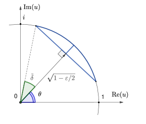
Figure 7: Geometric interpretation of constraints on complex numbers $u_{1}$ and $u_{2}$ appearing in Proposition 3.13. The region with blue boundary contains complex numbers $u$ that satisfy constraints $\mathrm{Re}\mathopen{}\left(ue^{-i\theta}\right)\mathclose{}\geq\sqrt{1-\epsilon/2}$ and $\mathopen{}\left|u\right|\mathclose{}\leq 1$. This region is split into two parts, an under-rotation region for $u_{1}$ with angular coordinates spanning $[\theta-\tilde{\delta},\theta]$ and an over-rotation region for $u_{2}$ with angular coordinates spanning $[\theta,\theta+\tilde{\delta}]$ for $\tilde{\delta}=\arcsin(\sqrt{\varepsilon/2})$.

As observed by [Campbell2017, Hastings2017], the constraints imposed by Proposition 3.13 admit quadratically better scaling in $\varepsilon$ as compared to approximation without mixing (Proposition 3.7), which would require $|r\cos(\delta)|\geq\sqrt{1-\varepsilon^{2}/4}$.

Evenly splitting the error as in Proposition 3.13 does not yield optimal solutions in general. A better approach is to first find a cheap (but possibly poor) approximation of the target. With the first approximation fixed, a search region for the second approximation can be defined. In particularly, this is useful when identity is a sufficiently good under-rotated or over-rotated approximation to the target rotation. This happens in practice when approximating Fourier angles. We give a detailed treatment in LABEL:appendix:optimal-mixing-solutions.

The main technical component of 3.12 is to show that the twirled mixture $p\mathcal{T}_{U_{1}}(\rho)+(1-p)\mathcal{T}_{U_{2}}(\rho)$ is equal to the target rotation $e^{i\theta Z}$ followed by a Pauli channel error.

Lemma 3.14 (Twirled mixture yields Pauli channel error).

Let $\theta$ be an angle, $U_{1},U_{2}$ be unitaries as in Equation 18 and $p$ be a probability as in Equation 20. Then

$$p\mathcal{T}_{U_{1}}(\rho)+(1-p)\mathcal{T}_{U_{2}}(\rho)=\mathcal{E}(\mathcal{Z}_{\theta}(\rho))$$ (27)

where $\mathcal{E}$ is a qubit Pauli channel

$$\mathcal{E}(\rho)=p\mathcal{P}_{r_{1},\delta_{1}}(\rho)+(1-p)\mathcal{P}_{r_{2},\delta_{2}}(\rho)$$ (28)

and

$$\mathcal{P}_{r,\delta}(\rho)=r^{2}\cos^{2}(\delta)\rho+\frac{1-r^{2}}{2}(X\rho X+Y\rho Y)+r^{2}\sin^{2}(\delta)Z\rho Z.$$ (29)

This lemma can be proved by calculating the four by four process matrices for channels induced by $U_{1}$, $U_{2}$, channels $\mathcal{T}_{U_{k}}$ and $\mathcal{E}$. Recall that for a qubit channel $\Psi$ the process matrix $\chi$ is given by

$$\Psi(\rho)=\sum_{P,Q\in\{I,X,Y,Z\}}\chi_{P,Q}P\rho Q.$$

The $\{Z,S\}$ twirl eliminates all but two off-diagonal elements and the mixture with probability $p$ eliminates the remaining off-diagonal elements. We then see that the process matrix of $\mathcal{E}$ is a diagonal matrix and therefore $\mathcal{E}$ is a Pauli channel. Finally we apply the following result from Section V.A in [Magesan2012] to get a closed form expression for the diamond norm distance between $\mathcal{E}$ and the identity channel:

Theorem 3.15 (Diamond norm distance between Pauli channels).

Suppose $\mathcal{E}_{1}$, $\mathcal{E}_{2}$ are $n$-qubit Pauli channels, that is

$$\mathcal{E}_{1}(\rho)=\sum_{P\in\{I,X,Y,Z\}^{\otimes n}}q_{P}P\rho P^{\dagger},\,\mathcal{E}_{2}(\rho)=\sum_{P\in\{I,X,Y,Z\}^{\otimes n}}r_{P}P\rho P^{\dagger},$$

then $\mathopen{}\left\|\mathcal{E}_{1}-\mathcal{E}_{2}\right\|\mathclose{}_{\diamond}=\sum_{P\in\{I,X,Y,Z\}^{\otimes n}}|q_{P}-r_{P}|$.

Detailed proofs of 3.14 and 3.12 are given in LABEL:sec:diamond-difference-twirled-mixture.

3.5 Mixed fallback approximation

The results of [Campbell2017, Hastings2017] halve the cost of qubit unitary approximation by taking probabilistic mixtures of unitaries. We show that an additional factor of two improvement in cost can be obtained by taking probabilistic mixtures of channels. In particular, we demonstrate a procedure for mixing fallback protocols (see Section 3.3). The basic idea is to apply at random one of two projective rotations, one that approximates $e^{i\theta Z}$ by over-rotation and one that approximates $e^{i\theta Z}$ by under-rotation. If the projective rotation fails, then a corresponding fallback channel is applied.

Problem 3.16 (Diagonal unitary approximation by projective rotation mixing).

Given:

• target angle $\theta$, a real number,

• success probability $q$, a positive real number between $0$ and $1$,

• gate set $G$, a finite set of two by two unitary matrices with determinant one,

• accuracy $\varepsilon$, a positive real number.

Find

• $G_{1},\ldots,G_{n}$, a sequence of sequences of elements of $G$ and

• $p_{1},\ldots,p_{n}$, a probability distribution

such that

• $|u_{k}|^{2}\geq q$ for all $k\in[n]$, and

• the diamond norm of the channel below is at most $\varepsilon$

  $$\sum_{k=1}^{n}p_{k}|u_{k}|^{2}\left(\mathcal{Z}_{\mathrm{Arg}(u_{k})}-\mathcal{Z}_{\theta}\right)$$

where $u_{k}$ is the top-left entry of the unitary $\mathopen{}\left(\begin{smallmatrix}u_{k}&-v_{k}^{\ast}\\ v_{k}&u_{k}^{\ast}\end{smallmatrix}\right)\mathclose{}$ corresponding to sequence $G_{k}$.

In analogy to Problem 3.11, this problem generalizes the projective rotation approximation problem (Problem 3.8) by allowing multiple projective rotation circuits in convex combination. Note that the elements of the probability distribution $p_{1},\ldots,p_{n}$ are distinct from the success probabilities of the projective rotations.

In the analysis of the fall-back protocol in 3.10 we considered only unitary fallback steps. We now consider fallbacks that are probabilistic mixtures of unitaries. The channel $\mathcal{F}$ for a fallback protocol has the form

$$\mathcal{F}(\rho)=q\mathcal{Z}_{\theta_{0}}(\rho)+(1-q)\mathcal{B^{\prime}}(\rho)$$ (30)

where $\mathcal{B^{\prime}}$ is the composition of the failure rotation $e^{i\theta_{1}Z}$ and the fallback step $\mathcal{B}$ and $q$ is the probability of success (measurement outcome of zero).

The following theorem provides a simple closed form bound for the diamond distance of a mixture of fallback protocols, similar to the expression obtained from 3.12 for unitary mixtures. The proof is provided in LABEL:sec:diamond-distance-fallback-mixture.

Theorem 3.17 (Diamond distance of a fallback mixture).

Let $\theta$ be an angle and let fallback channels

$$\mathcal{F}_{1}(\rho)=q_{1}\mathcal{Z}_{\theta+\delta_{1}}(\rho)+(1-q_{1})\mathcal{B}_{1}(\rho)$$ (31)

$$\mathcal{F}_{2}(\rho)=q_{2}\mathcal{Z}_{\theta+\delta_{2}}(\rho)+(1-q_{2})\mathcal{B}_{2}(\rho)$$ (32)

where $\sin(\delta_{1})\leq 0\leq\sin(\delta_{2})$. Define probability

$$p=\frac{q_{2}\sin(2\delta_{2})}{q_{2}\sin(2\delta_{2})-q_{1}\sin(2\delta_{1})}.$$ (33)

Then

$$\mathopen{}\left\|pq_{1}\left(\mathcal{Z}_{\theta+\delta_{1}}-\mathcal{Z}_{\theta}\right)+(1-p)q_{2}\left(\mathcal{Z}_{\theta+\delta_{2}}-\mathcal{Z}_{\theta}\right)\right\|\mathclose{}_{\diamond}=2\left(pq_{1}\sin^{2}(\delta_{1})+(1-p)q_{2}\sin^{2}(\delta_{2})\right)$$ (34)

and the total accuracy of the mixed fall-back approximation protocol is

$$||p\mathcal{F}_{1}+(1-p)\mathcal{F}_{2}-\mathcal{Z}_{\theta}||_{\diamond}\leq \,2\left(pq_{1}\sin^{2}(\delta_{1})+(1-p)q_{2}\sin^{2}(\delta_{2})\right)$$ (35)

$$+p(1-q_{1})||\mathcal{B}_{1}-\mathcal{Z}_{\theta}||_{\diamond}+(1-p)(1-q_{2})||\mathcal{B}_{2}-\mathcal{Z}_{\theta}||_{\diamond}.$$

The goal of a synthesis algorithm then is to bound Equation 35 by an approximation error $\varepsilon$. We have some flexibility in bounding the accuracy of the components of the two fallback protocols. We may set the accuracy of each term separately

$$2\left(pq_{1}\sin^{2}(\delta_{1})+(1-p)q_{2}\sin^{2}(\delta_{2})\right) =\varepsilon_{1}$$ (36)

$$p(1-q_{1})||\mathcal{B}_{1}-\mathcal{Z}_{\theta}||_{\diamond} =\varepsilon_{2}$$

$$(1-p)(1-q_{2})||\mathcal{B}_{2}-\mathcal{Z}_{\theta}||_{\diamond} =\varepsilon_{3}$$

$$\varepsilon_{1}+\varepsilon_{2}+\varepsilon_{3} \leq\varepsilon.$$

The first condition is ensured by solving 3.16. The second two conditions are ensured by solving the mixed diagonal approximation problems. Note that for the two fallback terms $||\mathcal{B}_{1}-\mathcal{Z}_{\theta}||_{\diamond}$ and $||\mathcal{B}_{2}-\mathcal{Z}_{\theta}||_{\diamond}$, the accuracy is scaled by $1-q_{1}$ and $1-q_{2}$ thereby reducing the fallback step approximation T-count on average by $1.5\log_{2}(1/(p(1-q_{1})))$ and $1.5\log_{2}(1/(1-p)/(1-q_{2}))$ when using mixed diagonal approximation with Clifford+$T$ gate set. This is in comparison to the cost of mixed diagonal approximation with Clifford+$T$ gate set of accuracy $\varepsilon$. As in previous sections, 3.16 is solved by finding gate sequences with certain constraints on the top-left entry of the unitaries they compute.

Proposition 3.18 (Projective rotation mixing approximation condition).

Suppose that we are given two sequences $G=g_{1},\dots,g_{n}$ and $H=h_{1},\dots,h_{m}$ from a gate set $G$. Define

$$g_{1}\dots g_{n}=\mathopen{}\left(\begin{array}[]{cc}u_{1}&-v_{1}^{\ast}\\ v_{1}&u_{1}^{\ast}\end{array}\right)\mathclose{},h_{1}\dots h_{n}=\mathopen{}\left(\begin{array}[]{cc}u_{2}&-v_{2}^{\ast}\\ v_{2}&u_{2}^{\ast}\end{array}\right)\mathclose{}.$$

Suppose that for angle $\theta$ and accuracy $\varepsilon$

• $u_{1}$ satisfies $\mathopen{}\left|u_{1}\right|\mathclose{}\geq\sqrt{q}$, $-\sqrt{\varepsilon/2}\leq\sin\mathopen{}\left(\mathrm{Arg}(u_{1})-\theta\right)\mathclose{}\leq 0$, and

• $u_{2}$ satisfies $\mathopen{}\left|u_{2}\right|\mathclose{}\geq\sqrt{q}$, $0\leq\sin\mathopen{}\left(\mathrm{Arg}(u_{2})-\theta\right)\mathclose{}\leq\sqrt{\varepsilon/2}$.

Then sequence $G,H$ and probability distribution $p,1-p$ for

$$p=\frac{q_{2}\sin(2\delta_{2})}{q_{2}\sin(2\delta_{2})-q_{1}\sin(2\delta_{1})},\text{ where }q_{k}=|u_{k}|^{2},\delta_{k}=\mathrm{Arg}(u_{k})-\theta$$ (37)

is a solution to the projective rotation mixing approximation Problem 3.16. For a geometric interpretation of the constraints on $u_{1},u_{2}$ see Figure 8.

Proof.

The conditions $|u_{1}|\geq\sqrt{q}$, $|u_{2}|\geq\sqrt{q}$ trivially ensure success probability conditions of Problem 3.16. We need to bound diamond distance of the channel

$$p|u_{1}|^{2}\left(\mathcal{Z}_{\mathrm{Arg}(u_{1})}-\mathcal{Z}_{\theta}\right)+(1-p)|u_{2}|^{2}\left(\mathcal{Z}_{\mathrm{Arg}(u_{2})}-\mathcal{Z}_{\theta}\right).$$

By Theorem 3.17 it is equal to

$$2\left(p|u_{1}|^{2}\sin^{2}(\delta_{1})+(1-p)|u_{2}|^{2}\sin^{2}(\delta_{2})\right)\leq 2\left(p\sin^{2}(\delta_{1})+(1-p)\sin^{2}(\delta_{2})\right)$$ (38)

$$\leq\varepsilon$$

∎

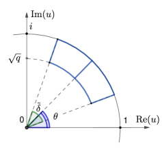
Figure 8: A geometric interpretation of constraints on the projective rotations given by Proposition 3.18. The sector with blue boundary contains complex numbers $u$ that satisfy constraints $\mathrm{Arg}\mathopen{}\left(u\right)\mathclose{}\in[\theta-\tilde{\delta},\theta+\tilde{\delta}]$ and $\mathopen{}\left|u\right|\mathclose{}\geq\sqrt{q}$, where $\tilde{\delta}=\arcsin(\sqrt{\varepsilon/2})$. This sector is split into two parts, an over-rotation sector for one projective rotation and an under-rotation sector for the other projective rotation.

The conditions $|\sin(\delta_{k})|\leq\sqrt{\varepsilon/2}$ imposed by Proposition 3.18 are quadratically looser than the equivalent condition for projective rotations without mixing (3.9) which requires $|\sin(\delta)|\leq\varepsilon/2$. When combined with unitary mixing for the fallback step, this yields a quadratic improvement in $\varepsilon$ for the entire fallback protocol. The gate cost of a fallback protocol scales as $C\log_{2}(1/\varepsilon)+O(1)$. Thus the quadratic improvement in $\varepsilon$ translates to a roughly two times savings in expected gate cost over conventional fallback protocols. For the more detailed cost comparisons see Table 1.

For reasonable ranges of $\varepsilon$ the $\log(1/\varepsilon)$ term is well below $100$, making additive constants and higher order terms an important consideration. In that sense, solutions obtained by Proposition 3.18 are sub-optimal. The overall cost can be optimized by a more careful assignment of $\varepsilon_{1},\varepsilon_{2}$ and $\varepsilon_{3}$ in Equation 36. This is discussed further in LABEL:appendix:optimal-mixing-solutions.

3.6 Mixed magnitude approximation

We have shown that taking a probabilistic mixture of channels leads to improvement in accuracy for diagonal approximations with and without the fallback protocol. It is natural to then question whether a similar improvement can be achieved for general unitary approximation. We show that this is indeed the case, following the same strategy of finding approximations corresponding to under- and over- rotations of a target angle.

We begin by defining the following problem for approximating an arbitrary X-rotation up to phases.

Problem 3.19 (Magnitude approximation by mixing).

Given:

• target angle $\theta$,

• gate set $G$, a finite set of two by two unitary matrices with determinant one,

• accuracy $\varepsilon$, a positive real number.

Find

• $G_{1},\ldots,G_{n}$, a sequence of sequences of elements of $G$ and

• $p_{1},\ldots,p_{n}$, a probability distribution on these sequences

such that

$$\left\|\sum_{k=1}^{n}p_{k}\mathcal{X}_{\arccos(\mathopen{}\left|u_{k}\right|\mathclose{})}-\mathcal{X}_{\theta}\right\|_{\diamond}\leq\varepsilon.$$

where $u_{k}$ is the top-left entry of the matrix corresponding to sequence $G_{k}$ and $\mathcal{X}_{\theta}$ is the channel induced by $e^{i\theta X}$.

As in Problem 3.11 and Problem 3.16, Problem 3.19 allows for a solution comprising a probabilistic mixture of channels. We can further assume without loss of generality that $\mathopen{}\left|\cos(\theta)\right|\mathclose{}\geq 1/\sqrt{2}$, by the following remark.

Remark 3.20.

Let $g_{1}\dots g_{n}$ be a solution to Problem 3.19 for target angle $\theta$. Then $iX\cdot g_{n}^{\dagger}\dots g_{1}^{\dagger}$ is a solution for target angle $\frac{\pi}{2}-\theta$, since $iX\cdot g_{n}^{\dagger}\dots g_{1}^{\dagger}=iXe^{-i\phi_{2}Z}(-iX)iXe^{-i\theta X}e^{-i\phi_{1}Z}=e^{i\phi_{2}Z}e^{i(\pi/2-\theta)X}e^{i\phi_{1}Z}.$

Hence, if $\mathopen{}\left|\cos(\theta)\right|\mathclose{}<1/\sqrt{2}$ we can simply apply magnitude approximation to $\pi/2-\theta$, noting that $\cos(\pi/2-\theta)=\sin(\theta)\geq 1/\sqrt{2}$.

The following proposition shows that the error bound on the diamond norm in Problem 3.19 induces a constraint on the top-left entries of the matrices corresponding to sequences $G_{k}$. Our approach is to again find X-approximations corresponding to under- and over-rotations of the angle $\delta$.

Proposition 3.21 (Mixed magnitude approximation condition).

Suppose we are given sequences $g_{1},\dots,g_{n}$ and $h_{1},\dots,h_{m}$ of gates from a gate set. Define complex numbers $u_{k},v_{k}$

$$g_{1}\dots g_{n}=\mathopen{}\left(\begin{array}[]{cc}u_{1}&-v_{1}^{\ast}\\ v_{1}&u_{1}^{\ast}\end{array}\right)\mathclose{},h_{1}\dots h_{m}=\mathopen{}\left(\begin{array}[]{cc}u_{2}&-v_{2}^{\ast}\\ v_{2}&u_{2}^{\ast}\end{array}\right)\mathclose{}$$

Suppose that for accuracy $\varepsilon$ and target angle $\theta$

• $\mathopen{}\left|u_{1}\right|\mathclose{}\in\{\cos(\theta^{\prime\prime}):\theta^{\prime\prime}\in[0,\pi/2],0\leq\theta-\theta^{\prime\prime}\leq\arcsin\sqrt{\varepsilon/2}\}$, and

• $\mathopen{}\left|u_{2}\right|\mathclose{}\in\{\cos(\theta^{\prime\prime}):\theta^{\prime\prime}\in[0,\pi/2],0\leq\theta^{\prime\prime}-\theta\leq\arcsin\sqrt{\varepsilon/2}\}$.

Define

$$p=\frac{\sin(2\delta_{2})}{\sin(2\delta_{2})-\sin(2\delta_{1})},\text{ where }\delta_{k}=\mathrm{arccos}(u_{k})-\theta$$

The the sequences $g_{1},\dots,g_{n}$ and $h_{1},\dots,h_{m}$ and probability distribution $p,1-p$ is a a solution to the magnitude mixing approximation Problem 3.19 with $n=2$, accuracy $\varepsilon$ and target angle $\theta$. For a geometric interpretation of the constraints on $|u_{k}|$ see Figure 9.

Proof.

Let $g_{1}\dots g_{n}=e^{i\phi_{1}Z}e^{i\theta_{u}X}e^{i\phi_{2}Z}$ with $\theta_{u}=\theta+\delta_{1}$ and $h_{1}\dots h_{m}=e^{i\psi_{1}Z}e^{i\theta_{o}X}e^{i\psi_{2}Z}$ with $\theta_{u}=\theta+\delta_{2}$. Then

$$\mathopen{}\left\|p\mathcal{X}_{\theta_{u}}+(1-p)\mathcal{X}_{\theta_{o}}-\mathcal{X}_{\theta}\right\|\mathclose{}_{\diamond}=\mathopen{}\left\|p\mathcal{Z}_{\theta_{u}}+(1-p)\mathcal{Z}_{\theta_{o}}-\mathcal{Z}_{\theta}\right\|\mathclose{}_{\diamond}.$$ (39)

using the identity $He^{i\theta Z}H=e^{i\theta X}$ and unitary invariance of the diamond norm (LABEL:prop:diamond-norm-unitary-invariance). The norm on the right hand side and the expression for $p$ are of the form required for Theorem 3.12, so we can conclude $\mathopen{}\left\|p\mathcal{X}_{\theta_{u}}+(1-p)\mathcal{X}_{\theta_{o}}-\mathcal{X}_{\theta}\right\|\mathclose{}_{\diamond}\leq\varepsilon$ when $2p(\sin^{2}(\delta_{1}))+2(1-p)(\sin^{2}(\delta_{2}))\leq\varepsilon$. It remain to show that $\sin^{2}(\delta_{k})\leq\varepsilon/2$.

Consider the under-rotated case. By definition $\mathopen{}\left|u_{1}\right|\mathclose{}=\cos(\theta_{u})$ and so $\theta-\theta_{u}\leq\arcsin\sqrt{\varepsilon/2}$. So we have $\sin^{2}(\delta_{1})\leq\varepsilon/2$ as required, and analogously for $\mathopen{}\left|u_{2}\right|\mathclose{}$. ∎

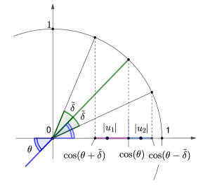
Figure 9: A geometric interpretation of constraints given by Proposition 3.21. Absolute values $\mathopen{}\left|u\right|\mathclose{}$ belonging to the interval $\{\cos(\delta^{\prime\prime}):\delta^{\prime\prime}\in[0,\frac{\pi}{2}],\mathopen{}\left|\delta^{\prime\prime}-\theta\right|\mathclose{}\leq\sqrt{\tilde{\delta}}\}$, for $\tilde{\delta}=\arcsin\sqrt{\varepsilon/2}$ are shown on the vertical axis. This interval is split into two parts, an over-rotation interval (blue) and an under-rotation interval (purple).

In comparison to Proposition 3.2, the constraint on the top-left matrix entries in Proposition 3.21 is quadratically looser, thus admitting a greater possible number of candidate values. Analogously to the unmixed case, mixed magnitude approximations can be extended to approximations of arbitrary unitaries.

Proposition 3.22 (General unitary approximation with mixing).

Let $U=e^{i\alpha Z}e^{i\theta X}e^{i\beta Z}$ be an arbitrary unitary in $SU(2)$. Let $g_{1},\dots,g_{n}$ and $h_{1},\dots,h_{m}$ be sequences from a gate set $G$ that satisfy the constraints of Proposition 3.21. Let probability $p$ be defined as in Proposition 3.21. Define angles $\phi_{k},\psi_{k}$ from equations $g_{1}\dots g_{n}=e^{i\phi_{1}Z}e^{i\theta_{u}X}e^{i\phi_{2}Z}$ and $h_{1}\dots h_{m}=e^{i\psi_{1}Z}e^{i\theta_{o}X}e^{i\psi_{2}Z}$. Suppose $\Phi_{1},\Phi_{2},\Psi_{1}$ and $\Psi_{2}$ are $\varepsilon$-approximations of $\mathcal{Z}_{\alpha-\phi_{1}},\mathcal{Z}_{\beta-\phi_{2}},\mathcal{Z}_{\alpha-\psi_{1}}$ and $\mathcal{Z}_{\beta-\psi_{2}}$, respectively. Then

$$\mathopen{}\left\|p\Phi_{1}\mathcal{G}\Phi_{2}+(1-p)\Psi_{1}\mathcal{H}\Psi_{2}-\mathcal{U}\right\|\mathclose{}_{\diamond}\leq 3\varepsilon,$$

where $\mathcal{G}$ and $\mathcal{H}$ are channels induced by products $g_{1}\cdots g_{n}$ and $h_{1}\cdots h_{m}$.

Proof.

Using the Euler decomposition of $U$ we have $\mathcal{U}=\mathcal{Z}_{\alpha}\mathcal{X}_{\theta}\mathcal{Z}_{\beta}$ and so

$$\mathopen{}\left\|p\Phi_{1}\mathcal{G}\Phi_{2}+(1-p)\Psi_{1}\mathcal{H}\Psi_{2}-\mathcal{U}\right\|\mathclose{}_{\diamond}=\mathopen{}\left\|p\Phi_{1}\mathcal{G}\Phi_{2}+(1-p)\Psi_{1}\mathcal{H}\Psi_{2}-\mathcal{Z}_{\alpha}\mathcal{X}_{\theta}\mathcal{Z}_{\beta}\right\|\mathclose{}_{\diamond}.$$

Applying the triangle inequality, we bound this norm from above by

$$p\mathopen{}\left\|\Phi_{1}\mathcal{G}\Phi_{2}-\mathcal{Z}_{\alpha}\mathcal{X}_{\theta_{u}}\mathcal{Z}_{\beta}\right\|\mathclose{}_{\diamond}+(1-p)\mathopen{}\left\|\Psi_{1}\mathcal{H}\Psi_{2}-\mathcal{Z}_{\alpha}\mathcal{X}_{\theta_{o}}\mathcal{Z}_{\beta}\right\|\mathclose{}_{\diamond}+\mathopen{}\left\|\mathcal{Z}_{\alpha}(p\mathcal{X}_{\theta_{u}}+(1-p)\mathcal{X}_{\theta_{o}}-\mathcal{X}_{\theta})\mathcal{Z}_{\beta}\right\|\mathclose{}_{\diamond}.$$

Now, using unitary invariance of the diamond norm with $e^{-i\alpha Z}$ and $e^{-i\beta Z}$, we can simplify the three terms in the expression above and bound each by an accuracy measure. Concretely, we obtain the following set of equations

$$p\mathopen{}\left\|\Phi_{1}\mathcal{G}\Phi_{2}-\mathcal{Z}_{\alpha}\mathcal{X}_{\theta_{u}}\mathcal{Z}_{\beta}\right\|\mathclose{}_{\diamond}=p\mathopen{}\left\|\Phi_{1}\underline{\mathcal{G}}\Phi_{2}-\mathcal{Z}_{\alpha}\mathcal{Z}_{-\phi_{1}}\underline{\mathcal{Z}_{\phi_{1}}\mathcal{X}_{\theta_{u}}\mathcal{Z}_{\phi_{2}}}\mathcal{Z}_{-\phi_{2}}\mathcal{Z}_{\beta}\right\|\mathclose{}_{\diamond}=\varepsilon_{1}$$

$$(1-p)\mathopen{}\left\|\Psi_{1}\mathcal{H}\Psi_{2}-\mathcal{Z}_{\alpha}\mathcal{X}_{\theta_{o}}\mathcal{Z}_{\beta}\right\|\mathclose{}_{\diamond}=(1-p)\mathopen{}\left\|\Psi_{1}\underline{\mathcal{H}}\Psi_{2}-\mathcal{Z}_{\alpha}\mathcal{Z}_{-\psi_{1}}\underline{\mathcal{Z}_{\psi_{1}}\mathcal{X}_{\theta_{o}}\mathcal{Z}_{\psi_{2}}}\mathcal{Z}_{-\psi_{2}}\mathcal{Z}_{\beta}\right\|\mathclose{}_{\diamond}=\varepsilon_{2}$$

$$\mathopen{}\left\|\mathcal{Z}_{\alpha}(p\mathcal{X}_{\theta_{u}}+(1-p)\mathcal{X}_{\theta_{o}}-\mathcal{X}_{\theta})\mathcal{Z}_{\beta}\right\|\mathclose{}_{\diamond}=\varepsilon_{3}.$$

such that the claim holds if $\varepsilon_{1}+\varepsilon_{2}+\varepsilon_{3}\leq 3\varepsilon.$ Consider the first norm $\mathopen{}\left\|\Phi_{1}\mathcal{G}\Phi_{2}-\mathcal{Z}_{\alpha}\mathcal{X}_{\theta_{u}}\mathcal{Z}_{\beta}\right\|\mathclose{}_{\diamond}$ and apply the chain rule

$$\mathopen{}\left\|\Phi_{1}\underline{\mathcal{G}}\Phi_{2}-\mathcal{Z}_{\alpha}\mathcal{Z}_{-\phi_{1}}\underline{\mathcal{Z}_{\phi_{1}}\mathcal{X}_{\theta_{u}}\mathcal{Z}_{\phi_{2}}}\mathcal{Z}_{-\phi_{2}}\mathcal{Z}_{\beta}\right\|\mathclose{}_{\diamond}\leq\mathopen{}\left\|\Phi_{1}-\mathcal{Z}_{\alpha-\phi_{1}}\right\|\mathclose{}_{\diamond}+$$ (40)

$$\mathopen{}\left\|\mathcal{G}-\mathcal{Z}_{\phi_{1}}\mathcal{X}_{\theta_{u}}\mathcal{Z}_{\phi_{2}}\right\|\mathclose{}_{\diamond}+\mathopen{}\left\|\Phi_{2}-\mathcal{Z}_{\beta-\phi_{2}}\right\|\mathclose{}_{\diamond}\leq 2\varepsilon$$

The same argument applies mutatis mutandis to $\mathopen{}\left\|\Psi_{1}\mathcal{H}\Psi_{2}-\mathcal{Z}_{\alpha}\mathcal{X}_{\theta_{o}}\mathcal{Z}_{\beta}\right\|\mathclose{}_{\diamond}$. Since the sequences $g_{1},\dots,g_{n}$ and $h_{1},\dots,h_{m}$ and $p$ satisfy Proposition 3.21 we also have

$$\mathopen{}\left\|\mathcal{Z}_{\alpha}(p\mathcal{X}_{\theta_{u}}+(1-p)\mathcal{X}_{\theta_{o}}-\mathcal{X}_{\theta})\mathcal{Z}_{\beta}\right\|\mathclose{}_{\diamond}=\mathopen{}\left\|p\mathcal{X}_{\theta_{u}}+(1-p)\mathcal{X}_{\theta_{o}}-\mathcal{X}_{\theta})\right\|\mathclose{}\leq\varepsilon.$$

Therefore $\varepsilon_{1}+\varepsilon_{2}+\varepsilon_{3}\leq 2\varepsilon p+2\varepsilon(1-p)+\varepsilon=3\varepsilon$.

∎

3.7 Geometric interpretations

In the sections above, we defined two methods for approximating diagonal unitaries: by direct unitary sequences (Problem 3.5), or by fallback protocols (3.8). Both of these methods can be extended by using probabilistic mixtures (Problem 3.11 and Problem 3.16). Each of these problems involves finding one or more sequences of gates that induce two-by-two unitary matrices of the form $\left(\begin{smallmatrix}u&-v^{*}\\ v&u^{*}\end{smallmatrix}\right)$. In each case, solutions can be described by conditions on the top-left entry $u$. See Proposition 3.7, Proposition 3.9, Proposition 3.13, and Proposition 3.18. Those conditions can be illustrated geometrically by regions on the complex plane: Figure 5 and Figure 6.

Figure 10 shows these regions overlayed one on top of another. This geometric illustration makes clear the progressive increase in solution space going from unitary approximation, to fallback approximation and then to probabilistic mixtures. The region areas for each approximation problem can be quickly computed using basic formulas for the areas of sectors and triangles. For instance, for diagonal approximation without mixing the region area is given by

$$\delta-\frac{1}{2}\sin(2\delta)$$

where $\delta$ is the angle subtending the minimal sector containing the region. The region areas are given to leading order of $\varepsilon$ in Table 4.

The projective approximation region encloses the unitary approximation region, provided that the probability of success $q$ satisfies a modest $q\leq 1-\varepsilon^{2}/4$. Loosely speaking, the condition $q=1-\varepsilon^{2}/4$ can be interpreted as the point at which the projection failure may be treated deterministically as an approximation error and no longer needs a fallback step.

Except for large values of $\varepsilon$, the unitary mixture region also encloses the (non-mixing) unitary approximation region. Finally, the projective mixing approximation region encloses all of the other regions, provided that $q\leq 1-\varepsilon/2$.

Indeed, for the chosen value of $\varepsilon=0.1$, the illustration in Figure 10 under-represents the relative difference in region sizes. Practical values of $\varepsilon$ are typically several orders of magnitude smaller, for which the relative difference in region sizes is dramatically larger. Figure 11 shows the areas of each of the approximation regions as a function of $\varepsilon$ and $q$.

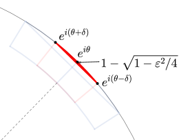
(a) Unitary region (Proposition 3.7) with area in $O(\varepsilon^{3})$

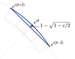
(b) Unitary mixing regions (Proposition 3.13) with area in $O(\varepsilon^{3/2})$

(c) Projective rotation region (Proposition 3.9) with area in $O(\varepsilon)$

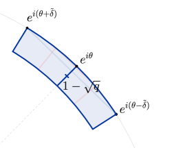
(d) Projective rotation mixing regions (Proposition 3.18) with area in $O(\varepsilon^{1/2})$

Figure 10: Approximation regions for target diagonal unitary $e^{i\theta Z}$. The figures above show close-ups of a section of the unit circle on the complex plane. Each colored highlight indicates a region of valid solutions for the corresponding approximation problem. For illustration, we have used (an impractical) approximation accuracy $\varepsilon=0.1$ and projective rotation success probability $q=0.9$. The unitary (a) and projective rotation (c) regions (without mixing) shown in red each subtend an angle of $2\delta=2\arcsin(\varepsilon/2)$. The unitary mixing (b) and projective rotation mixing (d) regions shown in blue each subtend an angle of $2\tilde{\delta}=2\arcsin(\sqrt{\varepsilon/2})$. The unitary mixing regions (b) fully encompasses the unitary region (a). Likewise, the projective rotation mixing region (d) fully encompasses the projective rotation region (c). For $q\leq 1-\varepsilon^{2}/4$, the projective rotation region (c) encompasses the unitary region (a). For $q\leq 1-\varepsilon/2$ the mixed projective regions encompasses all other regions.

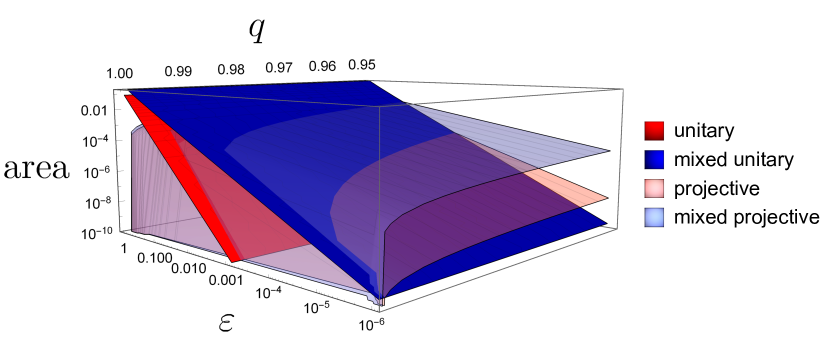
Figure 11: Areas of the solution regions prescribed by Proposition 3.7 (unitary), Proposition 3.13 (mixed unitary), Proposition 3.9 (projective) and Proposition 3.18 (mixed projective). Each curve shows the area of the region in the complex plane as a function of approximation accuracy $\varepsilon$ and success probability $q$. The unitary and projective areas, highlighted in red, scale quadratically with $\varepsilon$. The mixed unitary and mixed projective areas, highlighted in blue, scale linearly with $\varepsilon$. For all values of $\varepsilon$ and $q$ the mixed unitary (resp. projective) region has larger area than the corresponding non-mixed unitary (resp. projective) region, thereby admitting more candidate solutions. Except for large values of $\varepsilon$ and $q$, the projective and mixed projective regions have larger area then their respective unitary and mixed unitary regions.

Table 4: Region areas for unitary approximation problems with and without mixing. The geometric regions associated with each problem are illustrated in Figure 10. The diagonal and projective approximation problems result in two-dimensional regions, while the magnitude approximation problem results in a one-dimensional interval. In the latter case, Region area refers to the length of the interval. In all cases, it can be seen that the mixed version of the problem corresponds to a larger approximation region.

Approximation Problem	Region area (big-O)	Region area (with pre-factors)
Diagonal unitary approximation	$O(\varepsilon^{3})$	$\varepsilon^{3}/12+O(\varepsilon^{5})$
Mixed diagonal approximation	$O(\varepsilon^{3/2})$	$(2/3)(\varepsilon/2)^{3/2}+O(\varepsilon^{5/2})$
Projective rotation approximation	$O(\varepsilon)$	$(1-q)\varepsilon/2+O(\varepsilon^{3})$
Mixed projective approximation	$O(\varepsilon^{1/2})$	$(1-q)(\varepsilon/2)^{1/2}+O(\varepsilon^{3/2})$
Magnitude approximation	$O(\varepsilon)$	$\varepsilon/\sqrt{2}+O(\varepsilon^{3})$
Mixed magnitude approximation	$O(\varepsilon^{1/2})$	$\varepsilon^{1/2}+O(\varepsilon^{3/2})$

4 Solutions to approximation problems for common gate sets

In Section 3, we related solutions to various approximation problems to specific geometric regions. In this section, we specialize these results to a few specific gate sets. Unitaries that can be synthesized exactly with these gate sets define discrete subsets within the above convex bodies, and this naturally leads to an enumeration strategy to solve approximation problems. We first describe this approach for the V basis, the Clifford$+T$ basis and the Clifford$+\sqrt{T}$ basis, and we then generalize it to a family of gate sets introduced by [Kliuchnikov2015b] for diagonal approximation problems.

Throughout this section, we introduce the following notation to highlight common methodology across our three illustrative examples. We use $L$ to denote the field in which the entries of the unitaries defining a gate set lie, and $O_{L}$ to denote the integer ring of $L$. We associate a gate set determinant $\ell\in K$ to each gate set, such that any element generated by the gate set can be written as $\frac{1}{\sqrt{\ell^{N}}}\left(\begin{smallmatrix}u&-v^{*}\\ v&u^{*}\end{smallmatrix}\right)$ with $u,v\in O_{L}$ and $N\in\mathbb{Z}$. The determinant of a unitary with elements in $L$ lies in the maximal totally real subfield, which we denote by $K$. We have $L=K(i)$, where $i^{2}=-1$. The norm of an element in $L$ is a mapping from $L$ to $K$ defined by taking the product of an element of $L$ with its complex conjugate. We denote the ring of integers of $K$ by $O_{K}$. Finally, we make reference to objects known as orders. An order in a finite-dimensional algebra $M$ over $\mathbb{Q}$ is a subring of $M$ that is also a $\mathbb{Z}$-lattice, and which spans $M$ over $\mathbb{Q}$.

4.1 V basis

4.1.1 Quaternion maximal order

We recall that the V basis consists of the following six matrices:

$$V_{\pm Z} =\frac{1}{\sqrt{\ell}}\begin{pmatrix}1\pm 2i&0\\ 0&1\mp 2i\end{pmatrix}, V_{\pm Y} =\frac{1}{\sqrt{\ell}}\begin{pmatrix}1&\mp 2\\ \pm 2&1\end{pmatrix}, V_{\pm X} =\frac{1}{\sqrt{\ell}}\begin{pmatrix}1&\pm 2i\\ \pm 2i&1\end{pmatrix},$$

where $\ell=5$. Let $K=\mathbb{Q}$ and let $L=\mathbb{Q}(i)=\{a_{0}+ia_{1}:a_{0},a_{1}\in\mathbb{Q}\}$, where $i^{2}=-1$. Let $O_{K}=\mathbb{Z}$ and $O_{L}=\mathbb{Z}[i]=\{a_{0}+ia_{1}:a_{0},a_{1}\in\mathbb{Z}\}$ be the rings of integers of $K$ and $L$ respectively. Any element $t=a_{0}+ia_{1}\in O_{L}$ can be written as a 2-dimensional vector over $O_{K}$, namely $(a_{0},a_{1})$. There are two homomorphisms of $L$ into $\mathbb{C}$ related by complex conjugation. Denote by $\sigma$ the homomorphism such that $\sigma(i)=i$.

Let $M_{2}(L)$ be the algebra of all $2\times 2$ matrices with entries in $L$, and let $\mathcal{O}$ be an order in $M_{2}(L)$ that contains all the $V$ basis elements scaled by $\sqrt{\ell}$. For concreteness we will set

$$\mathcal{O}:=\mathbb{Z}\cdot I+\mathbb{Z}\cdot iX+\mathbb{Z}\cdot iY+\mathbb{Z}\cdot iZ.$$ (41)

We extend $\sigma$ over $\mathcal{O}$ in a natural way, namely for $M\in\mathcal{O}$ we define $\sigma(M)$ as the matrix whose elements are the images of the elements of $M$ under $\sigma$. As observed in [BGS, Kliuchnikov2015b], elements of $\mathcal{O}$ with determinant $\ell^{N}$ correspond to unitaries that can be expressed as a product of $N$ matrices from the V gate set via the map $\sigma^{\prime}(M)=\frac{1}{\sqrt{\ell^{N}}}\sigma(M)$.

Example 4.1.

Let $V=V_{Z}\cdot V_{X}=\frac{1}{5}\left(\begin{smallmatrix}1+2i&2i-4\\ 2i+4&1-2i\end{smallmatrix}\right)$. Then, $M_{V}=\left(\begin{smallmatrix}1+2i&2i-4\\ 2i+4&1-2i\end{smallmatrix}\right)=I+2\cdot iX-4\cdot iY+2\cdot iZ\in\mathcal{O}$ and $\sigma^{\prime}(M_{V})=V.$ Since $\det{(M_{V})}=5^{2},$ we have $N=2$ as expected, as $V$ is the product of two $V$ basis matrices. Note that the sequence $V_{Z}V_{X}$ cannot be simplified (over the V basis) so $N$ is minimal.