Coupling approaches for classical linear elasticity and bond-based peridynamic models

Abstract

Local-nonlocal coupling approaches provide a means to combine the computational efficiency of local models and the accuracy of nonlocal models. This paper studies the continuous and discrete formulations of three existing approaches for the coupling of classical linear elasticity and bond-based peridynamic models, namely 1) a method that enforces matching displacements in an overlap region, 2) a variant that enforces a constraint on the stresses instead, and 3) a method that considers a variable horizon in the vicinity of the interfaces. The performance of the three coupling approaches is compared on a series of one-dimensional numerical examples that involve cubic and quartic manufactured solutions. Accuracy of the proposed methods is measured in terms of the difference between the solution to the coupling approach and the solution to the classical linear elasticity model, which can be viewed as a modeling error. The objective of the paper is to assess the quality and performance of the discrete formulation for this class of force-based coupling methods.

1 Introduction

There has been, in the past few years, a great interest for the development of local-nonlocal coupling methods in order to take advantage, on the one hand, of the computational efficiency of local models and, on the other hand, of the accuracy of nonlocal models. We actually refer to the recent survey [6] for an overview and classification of generic local-nonlocal coupling methods. It is clear that the coupling of local and nonlocal models potentially have the following two benefits, namely the reduction of the computational cost in nonlocal modeling and a means to apply boundary conditions for nonlocal models. Indeed, nonlocal models such as peridynamics, molecular dynamics, or smoothed particle hydrodynamics, can be very computationally intensive, see e.g. [9]. However, they are often needed only in small regions, as it is the case when simulating cracks in computational mechanics, suggesting that one can consider a less expensive local model in the remainder of the domain. Moreover, a recent review [11] on the validation of peridynamics against actual experiments has revealed that one major challenge for using peridynamics lies in the treatment of the nonlocal boundary conditions [12, 21, 22, 15, 30, 41, 8, 7]. One can therefore imagine using local models all along the boundaries of the domain, for which boundary conditions can be unambiguously prescribed, and retaining the nonlocal models only in the interior of the domain by employing a coupling approach.

The paper focuses on approaches that couple the bond-based peridynamic model with the classical linear elasticity continuum model using a force-based coupling formulation. We refer again the reader to to [6] for the description of other types of coupling approaches such as optimization-based or energy-based methods. We adopt here, in order to establish the coupling methods, a deductive approach based on the coupling formulation of classical linear elasticity models in one dimension. This allows us to determine the minimal requirements when identifying the necessary constraints for matching the models. We thus identify the following three coupling methods, namely a method that matches the displacement in an overlap region of size given by the horizon of the peridynamic model and that we refer to as MDCM, a variant that matches stresses instead and that we call MSCM, and a method that introduces a variable horizon and that we refer to as VHCM. The first coupling method, i.e. MDCM, is in fact similar to the majority of the existing coupling approaches available in the literature [23, 17, 20, 38, 3, 19, 13, 14, 42, 43]. MSCM matches the stress field produced by the two models over a region of size defined by the horizon, as before, and features some similarities with the approach suggested in [34], apart from the discretization of the stress at the coupling interface. By contrast, VHCM, unlike MDCM and MSCM, avoids the introduction of an overlapping domain by scaling the horizon to zero when approaching the coupling interface, in a manner similar to [35, 24]. In all three cases, we formulate first the coupling methods at the continuous level and then propose discrete formulations based on the finite differences method, for the classical linear elasticity model, and the collocation method [27], for the peridynamic model. The advantages in doing so are twofold: first, to allow one to distinguish the discretization error from the modeling error and second, to be able to choose compatible numerical methods when discretizing the two models and the matching constraints. We note that coupling methods proposed in the literature are often introduced at the discrete level using the finite element method for the local model and a collocation approach for the nonlocal model.

We assess and compare the performance of the three coupling approaches on several numerical experiments dealing with the simulation of a one-dimensional bar. We show that the three methods produce the same error-free solution, as expected, on problems involving manufactured cubic polynomial solutions. However, the numerical results provided by the three methods are different when the manufactured solution for the linear elasticity problem is given by a polynomial function of degree at least four. We then measure the accuracy of the proposed methods in terms of the modeling error, which is defined as the difference between the solution to the classical linear elasticity problem and the solution to each coupled problem. We then perform some $\delta$-convergence and $m$-convergence analyses in order to evaluate the potential of each coupling approach.

The paper is organized as follows. Section 2 introduces the model problem and some preliminaries. Section 3 describes the continuous formulation of the coupling between classical linear elasticity models in one dimension. Section 4 presents the three coupling approaches for the classical linear elasticity and peridynamic models at the continuous level. Section 5 provides the discrete formulations and detailed algorithms of the coupling methods based on the finite differences and collocation methods. Section 6 describes the numerical examples including $\delta$-convergence and $m$-convergence studies. Finally, Section 7 concludes the paper.

2 Model problem and preliminaries

The model problem will consist in studying the static equilibrium of a bar held fixed at one end and subjected to a longitudinal traction at the other end. We shall suppose here that the deformations in the bar are infinitesimally small and can be adequately described by the theory of linear elasticity. Moreover, we assume for simplicity that the bar has a unit cross-sectional area $A=1$. We present below the local model based on classical elasticity theory and the non-local model counterpart derived from the linearized bond-based peridynamic theory [36].

2.1 Classical linear elasticity model

Let $\Omega=(0,\ell)\subset\mathbb{R}$ and $\overline{\Omega}$ be the closure of $\Omega$, i.e. $\Omega=[0,\ell]$. The continuum local problem consists in finding the displacement $\underline{u}\in\overline{\Omega}$ such that:

$$-E\underline{u}^{\prime\prime}(x)=f_{b}(x), \quad\forall x\in\Omega,$$ (1)

$$\underline{u}(x)=0, \quad\text{at}\ x=0,$$ (2)

$$E\underline{u}^{\prime}(x)=g, \quad\text{at}\ x=\ell,$$ (3)

where $E$ is the constant modulus of elasticity of the bar, $f_{b}=f_{b}(x)$ is a scalar function describing the external body force density (per unit length), and $g\in\mathbb{R}$ is the traction force applied at end point $x=\ell$. We will work with the mixed boundary value problem for most of the theoretical development to be as general as possible, but will also consider in the numerical examples some problems with homogeneous Dirichlet conditions at both ends, replacing the Neumann boundary condition (3) by the Dirichlet boundary condition $u(\ell)=0$. We also suppose that $f_{b}$ is chosen sufficiently smooth so that regularity in the solution is not an issue when comparing the solutions from the two models. Note that we use the notation $\underline{u}$ for the solution to the classical elasticity problem in order to emphasize that it may be different from the peridynamic solution $u$ introduced below.

2.2 Peridynamic model

Our objective will be to replace the local model by the peridynamic model in a subregion of $\Omega$. Let $\delta>0$ denote the so-called horizon of the peridynamic model and let $H_{\delta}(x)=(x-\delta,x+\delta)$ be the subdomain of the neighboring particles within the horizon. Because of the nonlocal nature of the model, we can only consider subregions $\Omega_{\delta}=(a,b)$ such that $a>\delta$ and $b<\ell-\delta$. In that case, we observe that for any given point $x$ in the interval $\Omega_{\delta}$, we have that $H_{\delta}(x)\subset\Omega$, as show in Figure 1. The general formulation, in one or higher dimension, of the linearized microelastic model [36] is given by:

$$-\int_{H_{\delta}(x)}\kappa\frac{\xi\otimes\xi}{\|\xi\|^{3}}(u(y)-u(x))dy=f_{b}(x),$$ (4)

where $\kappa$ is the parameter that characterizes the stiffness of the “bonds” between point $x$ and the neighboring points $y\in H_{\delta}(x)$, $\xi$ is the vector between two material points in the reference configuration, i.e. $\xi=y-x$, $\|\xi\|$ is the Euclidean norm of vector $\xi$, and $u(x)$ is the displacement of $x$ in the deformed configuration. In the case of the one-dimensional bar, the above integral at a point $x\in\Omega_{\delta}$ can be rewritten as:

$$-\int_{x-\delta}^{x+\delta}\kappa\frac{u(y)-u(x)}{|y-x|}dy=f_{b}(x).$$ (5)

Figure 1: Definition of the computational domains for the peridynamic model.

We now identify the material parameter $\kappa$ such that the solution of the linearized microelastic peridynamic model is compatible with that of the continuum local model. One may do so by matching the strain energy of the two models [36]. Alternatively, one can recover equation (1) from (5) by taking the limit $\delta\rightarrow 0$. Supposing that the displacement $u(x)$ is sufficiently smooth, the Taylor expansion of $u(y)$ around $x$ yields, for $y\in\Omega_{\delta}$,

$$u(y)-u(x)=u^{\prime}(x)(y-x)+\frac{1}{2}u^{\prime\prime}(x)(y-x)^{2}+\frac{1}{6}u^{\prime\prime\prime}(x)(y-x)^{3}+\frac{1}{24}u^{\prime\prime\prime\prime}(x)(y-x)^{4}+\ldots$$ (6)

Substituting (6) for $u(y)-u(x)$ in the integral in (5), one gets:

$$\int_{x-\delta}^{x+\delta}\kappa\frac{u(y)-u(x)}{|y-x|}dy=\frac{\kappa\delta^{2}}{2}\Big{(}u^{\prime\prime}(x)+\frac{\delta^{2}}{24}u^{\prime\prime\prime\prime}(x)+\ldots\Big{)},$$ (7)

so that (5) becomes:

$$-\frac{\kappa\delta^{2}}{2}\Big{(}u^{\prime\prime}(x)+\frac{\delta^{2}}{24}u^{\prime\prime\prime\prime}(x)+\ldots\Big{)}=f_{b}(x),\quad\forall x\in\Omega_{\delta}.$$ (8)

By taking the limit when $\delta\rightarrow 0$, one then recovers the differential equation (1) pointwise whenever $\kappa$ is chosen as:

$$\frac{\kappa\delta^{2}}{2}=E,\quad\text{that is}\ \kappa=\frac{2E}{\delta^{2}},$$ (9)

in agreement with [32]. However, if $\delta$ is kept finite, the value $\kappa=2E/\delta^{2}$ will always induce a modeling error between the solutions of the peridynamic and linear elasticity models, unless all derivatives $u^{(k)}$ of order $k\geq 4$ of the displacement field $u$ vanish for all $x\in\Omega_{\delta}$. In other words, this is a well known fact that the peridynamic and local models are fully compatible if $u(x)$ is a polynomial function of degree at most three. We shall say that the peridynamic model provides an approximation of the linear elasticity model with a degree of precision equal to three with respect to the parameter $\delta$. Our goal will be to build coupling methods whose degree of precision will also be three.

The challenging issue is that the degree of precision decreases as soon as the integral in (5) is evaluated over subdomains of $H_{\delta}(x)$, which is the case when $x$ approaches boundaries or interfaces. This is related to the so-called skin effect [4]. Indeed, truncation of the set $H_{\delta}(x)$ close to a boundary induces forces involving the first derivative of $u$. For example, following [36, 26], we can introduce the stress at a point $x$ in the domain as:

$$\sigma^{\pm}(u)(x)=\int_{x-\delta}^{x}\int_{x}^{z\pm\delta}\kappa\frac{u(y)-u(z)}{|y-z|}dydz,$$ (10)

and show, using the Taylor expansion (6) as before and substituting $E$ for $\kappa\delta^{2}/2$, that:

$$\sigma^{\pm}(u)(x)=Eu^{\prime}(x)+\frac{E\delta^{2}}{24}u^{\prime\prime\prime}(x)+\mathcal{O}(\delta^{3}).$$

We thus observe that these integral quantities are second-order approximations of the stress $Eu^{\prime}(x)$ with respect to $\delta$ with a degree of precision of two. In other words, $\sigma^{\pm}(u)$ provide the exact value of $Eu^{\prime}$ at point $x$ whenever $u$ is quadratic in the neighborhood of $x$. In order to obtain approximations with a degree of precision of three, one needs to include the higher-order term such that:

$$\sigma^{\pm}(u)(x)=\frac{\delta}{2}\int_{x-\delta}^{x}\int_{x}^{z\pm\delta}\kappa\frac{u(y)-u(z)}{|y-z|}dydz-\frac{\kappa\delta^{4}}{48}u^{\prime\prime\prime}(x).$$ (11)

Now, if $u$ is cubic in the neighborhood of $x$, $\sigma^{\pm}(u)$ lead to the exact value of $Eu^{\prime}$ at $x$. We will see how these results will become useful when building the coupling methods. We also note that one could consider alternative definitions of the stress at a point $x$ computed from the peridynamic model.

3 Coupling of linear elasticity models

The purpose of this section is to review the general coupling formulation in the case of two classical linear elasticity models and to study the particular setting where the classical equation (1) is replaced by (8). We will also introduce a modified formulation in which the pointwise interfaces are replaced by overlapping regions between the two models.

3.1 General formulation

We suppose here that we are interested in coupling linear elasticity models. We thus partition domain $\Omega$ into the subdomains $\Omega_{1}=(0,a)\cup(b,\ell)$ and $\Omega_{2}=(a,b)$, where we consider the first model in $\Omega_{1}$, with modulus of elasticity $E_{1}$, and the second model in $\Omega_{2}$, with $E_{2}$. The configuration is shown in Figure 2. It is well-known that the coupled model consists in this case in solving for $\underline{u}_{1}$ in $\overline{\Omega}_{1}$ and $\underline{u}_{2}$ in $\overline{\Omega}_{2}$ such that:

$$-E_{1}\underline{u}_{1}^{\prime\prime}(x) =f_{b}(x),\quad\forall x\in\Omega_{1},$$ (12)

$$-E_{2}\underline{u}_{2}^{\prime\prime}(x) =f_{b}(x),\quad\forall x\in\Omega_{2},$$

with boundary conditions:

$$\underline{u}_{1}(x) =0,\quad\text{at}\ x=0,$$ (13)

$$E_{1}\underline{u}_{1}^{\prime}(x) =g,\quad\text{at}\ x=\ell,$$

and interface conditions:

$$\underline{u}_{1}(x)-\underline{u}_{2}(x) =0,\quad\text{at}\ x=a\ \text{and}\ x=b,$$ (14)

$$E_{1}\underline{u}_{1}^{\prime}(x)-E_{2}\underline{u}_{2}^{\prime}(x) =0,\quad\text{at}\ x=a\ \text{and}\ x=b,$$

where the last two equations correspond to the continuity of the displacement and the stress at the pointwise interfaces.

Figure 2: Definition of the computational domains for the coupling of two linear elasticity models.

3.2 Examples

In this section, we analyze the solution to the above coupling problem when the model equation in $\Omega_{2}$ is actually replaced by the differential equation (8) arising from the peridynamic model. We consider the special case when the exact solution is a quartic polynomial with constant fourth derivative equal to $\lambda$. For the sake of simplicity, we shall slightly modify the notation as $\underline{u}_{1}(x)=\underline{u}(x)$, $E_{1}=E$, $\underline{u}_{2}(x)=u(x)$, $E_{2}=E=\kappa\delta^{2}/2$, so that the problem reads:

$$-E\underline{u}^{\prime\prime}(x)=f_{b}(x), \quad\forall x\in\Omega_{1},$$ (15)

$$-Eu^{\prime\prime}(x)-E\frac{\delta^{2}}{24}\lambda=f_{b}(x), \quad\forall x\in\Omega_{2},$$

$$\underline{u}(x)=0, \quad\text{at}\ x=0,$$

$$E\underline{u}^{\prime}(x)=g, \quad\text{at}\ x=\ell,$$

$$\underline{u}(x)-u(x)=0, \quad\text{at}\ x=a\ \text{and}\ x=b,$$

$$E\underline{u}^{\prime}(x)-Eu^{\prime}(x)=0, \quad\text{at}\ x=a\ \text{and}\ x=b.$$

Since all equations are linear here, the above problem can be recast, using the superposition principle, as that of searching for the function $v=v(x)$, for all $x\in\overline{\Omega}$, such that:

$$-Ev^{\prime\prime}(x)=0, \quad\forall x\in\Omega_{1},$$ (16)

$$-Ev^{\prime\prime}(x)=E\frac{\delta^{2}}{24}\lambda, \quad\forall x\in\Omega_{2},$$

$$v(x)=0, \quad\text{at}\ x=0,$$

$$Ev^{\prime}(x)=0, \quad\text{at}\ x=\ell,$$

$$v(x^{-})-v(x^{+})=0, \quad\text{at}\ x=a\ \text{and}\ x=b,$$

$$Ev^{\prime}(x^{-})-Ev^{\prime}(x^{+})=0, \quad\text{at}\ x=a\ \text{and}\ x=b.$$

where $x^{-}=\lim_{\epsilon\to 0}(x-\epsilon)$ and $x^{+}=\lim_{\epsilon\to 0}(x+\epsilon)$, with $\epsilon>0$. The function $v$ corresponds to the difference between the solution pair $(\underline{u},u)$ of the coupling problem (15) and the solution $\underline{u}$ to the linear elasticity problem (1) over the whole domain $\Omega$. The general solution is then given by:

$$v(x)=\left\{\begin{aligned} &C_{1}x+C_{2},&&\quad\forall x\in[0,a]\\ &-\frac{\lambda\delta^{2}}{48}x^{2}+C_{3}x+C_{4},&&\quad\forall x\in[a,b]\\ &C_{5}x+C_{6},&&\quad\forall x\in[b,\ell]\end{aligned}\right.$$ (17)

Upon applying the boundary and interface conditions, one obtains the solution:

$$v_{N}(x)=\left\{\begin{aligned} &\frac{\lambda\delta^{2}}{24}(b-a)x,&&\quad\forall x\in[0,a]\\ &\frac{\lambda\delta^{2}}{48}\big{(}b^{2}-a^{2}-(b-x)^{2}\big{)},&&\quad\forall x\in[a,b]\\ &\frac{\lambda\delta^{2}}{48}(b^{2}-a^{2}),&&\quad\forall x\in[b,\ell]\end{aligned}\right.$$ (18)

We also consider the problem with homogeneous Dirichlet conditions at both ends, replacing the Neumann condition $E\underline{u}^{\prime}(\ell)=g$ by $\underline{u}(\ell)=0$, all other equations in (15) remaining the same. In that case, the solution $v(x)$ reads:

$$v_{D}(x)=\left\{\begin{aligned} &\frac{\lambda\delta^{2}}{48}\frac{(b-a)}{\ell}\big{(}2\ell-(a+b)\big{)}x,&&\quad\forall x\in[0,a]\\ &\frac{\lambda\delta^{2}}{48}\Big{(}\big{(}b^{2}-a^{2}\big{)}\frac{\ell-x}{\ell}-(b-x)^{2}\Big{)},&&\quad\forall x\in[a,b]\\ &\frac{\lambda\delta^{2}}{48}\big{(}b^{2}-a^{2}\big{)}\frac{\ell-x}{\ell},&&\quad\forall x\in[b,\ell]\end{aligned}\right.$$ (19)

We illustrate in Figure 3 the solutions (18) and (19) for particular values of the data, i.e. $a=1$, $b=2$, $b=3$, and $\delta=1/8$. Moreover, for (18), we suppose that the exact solution to the classical linear elasticity problem is given by $\underline{u}(x)=x^{4}$, so that $\lambda=24$, while for (19), we take $\underline{u}(x)=x^{2}(144-96x+16x^{2})/81$, so that $\lambda=128/27$. We observe in Figure 3 that the solution (18) in the interval $[b,\ell]=[2,3]$ remains constant, which corresponds to the maximum value of $v_{N}$ over the whole domain $[0,\ell]=[0,3]$:

$$v_{N,\max}=\frac{\lambda\delta^{2}}{48}(b^{2}-a^{2})=\frac{3}{2}\delta^{2}.$$ (20)

As far as the solution $v_{D}$ (19) is concerned, it reaches its maximum value in the interval $[a,b]$, and more specifically at $x=b-(b^{2}-a^{2})/(2\ell)$. Then

$$v_{D,\max}=\frac{\lambda\delta^{2}}{48}(b^{2}-a^{2})\frac{4\ell^{2}-4b\ell+b^{2}-a^{2}}{4\ell^{2}}=\frac{10}{81}\delta^{2}.$$ (21)

We will use these quantities to assess the the efficiency of the coupling methods between classical linear elasticity and peridynamic models in the numerical examples of Section 6.

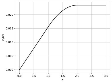
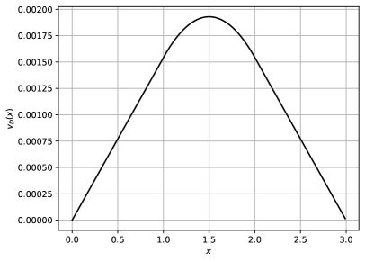
Figure 3: Illustration of the solutions $V_{N}$ (18) and $v_{D}$ (19) with $a=1$, $b=2$, $b=3$, and $\delta=1/8$. For $V_{N}$, shown on the left, $\underline{u}(x)=x^{4}$, implying $\lambda=24$, and for $V_{D}$, $\underline{u}(x)=x^{2}(144-96x+16x^{2})/81$ so that $\lambda=128/27$.

3.3 Modified formulation

In the particular case where $E_{1}=E_{2}=E$, the condition of stress continuity at the pointwise interfaces $x=a$ and $x=b$ can be replaced by a constraint involving the displacements on overlap regions between the two domains $\Omega_{1}$ and $\Omega_{2}$. In order to do so, we consider the overlap regions $\Gamma_{a}$ and $\Gamma_{b}$, both of size $\varepsilon$, as shown in Figure 2. The above problem can then be recast as finding $\underline{u}_{1}$ in $\overline{\Omega}_{1}$ and $\underline{u}_{2}$ in $\overline{\Omega_{2}\cup\Gamma_{a}\cup\Gamma_{b}}$ such that:

$$-E\underline{u}_{1}^{\prime\prime}(x)=f_{b}(x), \quad\forall x\in\Omega_{1},$$ (22)

$$-E\underline{u}_{2}^{\prime\prime}(x)=f_{b}(x), \quad\forall x\in\text{Int}\big{(}\overline{\Omega_{2}\cup\Gamma_{a}\cup\Gamma_{b}}\big{)}=(a-\varepsilon,b+\varepsilon),$$

$$\underline{u}_{1}(x)=0, \quad\text{at}\ x=0,$$

$$E\underline{u}_{1}^{\prime}(x)=g, \quad\text{at}\ x=\ell,$$

$$\underline{u}_{1}(x)-\underline{u}_{2}(x)=0, \quad\text{at}\ x=a\ \text{and}\ x=b$$

$$\underline{u}_{1}(x-\varepsilon)-\underline{u}_{2}(x-\varepsilon)=0, \quad\text{at}\ x=a$$

$$\underline{u}_{1}(x+\varepsilon)-\underline{u}_{2}(x+\varepsilon)=0, \quad\text{at}\ x=b.$$

The above problem, and in particular the last two equations, ensure that $\underline{u}_{1}(x)=\underline{u}_{2}(x)$, for all $x\in\Gamma_{a}\cup\Gamma_{b}$. This naturally implies that $\underline{u}_{1}^{\prime}(a)=\underline{u}_{2}^{\prime}(a)$ and $\underline{u}_{1}^{\prime}(b)=\underline{u}_{2}^{\prime}(b)$, which allows one to recover the interface conditions $E\underline{u}_{1}^{\prime}(x)-E\underline{u}_{2}^{\prime}(x)=0$, at $x=a$ and $x=b$, as required by (14). However, this coupling problem would clearly provide an incorrect solution if $E_{1}\neq E_{2}$. This observation will become relevant when we attempt to couple classical linear elasticity and peridynamic models, since the latter is not exactly equivalent to the former in the case of finite horizon $\delta$.

4 Coupling of classical linear elasticity and peridynamic models

The main challenge when employing a peridynamic model of constant horizon $\delta$ is that it is necessary to extend the domain $\Omega_{\delta}$ by extra layers of size $\delta$ in order to be able to correctly estimate the integral term in the vicinity of the boundaries. One objective in coupling peridynamics with classical linear elasticity is therefore to recover, from the linear elasticity solution, compatible displacements in those layers that can be used in the peridynamic model. As before, we introduce two points $a$ and $b$ inside $\Omega=(0,\ell)$ such that $a<b$ and define the subdomains $\Omega_{e}=(0,a)\cup(b,\ell)$ and $\Omega_{\delta}=(a,b)$, as shown in Figure 4. We also consider the so-called overlapping domains $\Gamma_{a}=(a-\delta,a)$ and $\Gamma_{b}=(b,b+\delta)$ of size $\delta$. Following the discussion of the previous section, we propose two approaches to construct compatible displacements from the linear elasticity solution over the overlapping regions $\Gamma_{a}$ and $\Gamma_{b}$. Alternatively, in order to avoid extending the peridynamic region $\Omega_{\delta}$, one could consider a peridynamic model with variable horizon such that $\delta$ goes to zero when approaching the boundaries of the domain. This will be the basis of a third coupling approach presented below.

Figure 4: Definition of the computational domains for the coupling between a linear elasticity model and a peridynamic model.

4.1 Coupling method with matching displacements (MDCM)

In the first approach, we choose to constrain the displacements from the two models to match in $\Gamma_{a}$ and $\Gamma_{b}$. The problem consists in finding $\underline{u}\in\overline{\Omega}_{e}$ and $u\in\overline{\Omega_{\delta}\cup\Gamma_{a}\cup\Gamma_{b}}$ such that:

$$-E\underline{u}^{\prime\prime}(x)=f_{b}(x), \quad\forall x\in\Omega_{e},$$ (23)

$$-\int_{x-\delta}^{x+\delta}\kappa\frac{u(y)-u(x)}{|y-x|}dy=f_{b}(x), \quad\forall x\in\overline{\Omega}_{\delta},$$

$$\underline{u}(x)=0, \quad\text{at}\ x=0,$$

$$E\underline{u}^{\prime}(x)=g, \quad\text{at}\ x=\ell,$$

$$u(x)-\underline{u}(x)=0, \quad\forall x\in\overline{\Gamma_{a}\cup\Gamma_{b}}.$$

The above formulation has a degree of precision of three with respect to the parameter $\delta$ and should provide the exact solution given by the classical linear elasticity model as long as the solution is a polynomial function of degree up to three. However, the two models are not compatible anymore when the solution is a polynomial of higher degree and one should expect errors due to the matching of the displacements in the overlapping regions. This approach is similar in essence, up to some slight variations, to the methods proposed in [5, 42] and is inspired by (22).

4.2 Coupling method with matching stresses (MSCM)

In the second approach, we choose to constrain the stresses from the two models in the overlapping regions. We then search for $\underline{u}\in\overline{\Omega}_{e}$ and $u\in\overline{\Omega_{\delta}\cup\Gamma_{a}\cup\Gamma_{b}}$ such that:

$$-E\underline{u}^{\prime\prime}(x)=f_{b}(x), \quad\forall x\in\Omega_{e},$$ (24)

$$-\int_{x-\delta}^{x+\delta}\kappa\frac{u(y)-u(x)}{|y-x|}dy=f_{b}(x), \quad\forall x\in\Omega_{\delta},$$

$$\underline{u}(x)=0, \quad\text{at}\ x=0,$$

$$E\underline{u}^{\prime}(x)=g, \quad\text{at}\ x=\ell,$$

$$u(x)-\underline{u}(x)=0, \quad\text{at}\ x=a\ \text{and}\ x=b,$$

$$\sigma^{+}(u)(x)-E\underline{u}^{\prime}(x)=0, \quad\forall x\in\overline{\Gamma}_{a},$$

$$\sigma^{-}(u)(x)-E\underline{u}^{\prime}(x)=0, \quad\forall x\in\overline{\Gamma}_{b},$$

where $\sigma^{\pm}(u)$ could be given by either (10) or (11). However, in order to preserve the degree of precision of three for the coupling approach, one needs to approximate the stresses $\sigma^{\pm}(u)$ by (11). We remark that this approach is more akin to the general formulation (12)-(14) for coupling classical linear elasticity models, in the sense that the continuity of the stress at the interfaces should be better approximated than in the first coupling method (23). This will be indeed confirmed by the numerical examples. This approach is inspired by [34].

4.3 Coupling method with variable horizon (VHCM)

The objective here is to introduce a formulation of the peridynamic model in which the horizon $\delta$ is allowed to vary within the domain $\Omega_{\delta}$, in such a way that the horizon should tend to zero as one approaches the interfaces $x=a$ and $x=b$ while remaining constant inside $\Omega_{\delta}$ sufficiently far from the interfaces. In that way, the peridynamic model would naturally converge to the classical linear elasticity model when approaching the coupling region and it would be unnecessary to consider overlapping domains.

Following [30], given $\delta\in\mathbb{R}^{+}$, the variable horizon $\delta_{v}(x)$ should thus satisfy the following requirements:

$$0\leq\delta_{v}(x)\leq\delta,\qquad\delta_{v}(x)\leq x-a,\qquad\delta_{v}(x)\leq b-x,\qquad\forall x\in\Omega_{\delta}=(a,b).$$ (25)

The choice of the function $\delta_{v}(x)$ is obviously not unique. However, the simplest continuous function that fulfill these requirements is the piecewise linear function shown in Figure 5:

$$\delta_{v}(x)=\left\{\begin{array}[]{ll}x-a,&\quad a<x\leq a+\delta,\\ \delta,&\quad a+\delta<x\leq b-\delta,\\ b-x,&\quad b-\delta<x<b.\end{array}\right.$$ (26)

Alternative functions, in particular smoother functions, could also be considered as long as they satisfy the above requirements. In view of (9), the horizon being a function of $x$ implies that the material parameter $\kappa$ should also depend on $x$, i.e. $\kappa=\bar{\kappa}(x)$, if the non-local model is to be compatible with the classical linear elasticity model, so that (5) should now read

$$-\int_{x-\delta_{v}(x)}^{x+\delta_{v}(x)}\bar{\kappa}(x)\frac{u(y)-u(x)}{|y-x|}dy=f_{b}(x),\quad\forall x\in\Omega_{\delta}.$$ (27)

Compatibility of the two models everywhere with a convergence of order $\mathcal{O}(\delta^{2})$ implies that the quantity $\bar{\kappa}(x)\delta_{v}^{2}(x)$ should remain constant for all $x\in\Omega_{\delta}$, i.e. with $\kappa$ satisfying (9), one has

$$\bar{\kappa}(x)\delta_{v}^{2}(x)=\kappa\delta^{2},\quad\forall x\in\Omega_{\delta}.$$ (28)

The coupling method with variable horizon is based on the general formulation (12)-(14) and consists in finding $\underline{u}\in\overline{\Omega}_{e}$ and $u\in\overline{\Omega}_{\delta}$ such that:

$$-E\underline{u}^{\prime\prime}(x)=f_{b}(x), \quad\forall x\in\Omega_{e},$$ (29)

$$-\int_{x-\delta_{v}(x)}^{x+\delta_{v}(x)}\bar{\kappa}(x)\frac{u(y)-u(x)}{|y-x|}dy=f_{b}(x), \quad\forall x\in\Omega_{\delta},$$

$$\underline{u}(x)=0, \quad\text{at}\ x=0,$$

$$E\underline{u}^{\prime}(x)=g, \quad\text{at}\ x=\ell,$$

$$u(x)-\underline{u}(x)=0, \quad\text{at}\ x=a\ \text{and}\ x=b,$$

$$\sigma^{+}(u)(x)-E\underline{u}^{\prime}(x)=0, \quad\text{at}\ x=a,$$

$$\sigma^{-}(u)(x)-E\underline{u}^{\prime}(x)=0, \quad\text{at}\ x=b.$$

The main advantage of this approach in regards to the other two coupling methods is that it does not involve any overlapping domains, which should simplify its implementation. Moreover, its degree of precision should be three as long as the stresses $\sigma^{\pm}(u)$ are approximated by (11). This approach is inspired by [35, 24].

Figure 5: Example of a variable horizon function $\delta_{v}(x)$. The circles centered at points $x\in(a,a+\delta)$ are representations of the associated domains $H_{\delta}(x)$ in terms of $\delta_{v}(x)$.

5 Discretization

We have introduced in the previous section the continuous formulation of three coupling methods based on the coupling of elasticity models as described in Section 3. We are now in a position to provide the discrete formulations of those coupling problems. For the sake of simplicity, we choose here to discretize the peridynamic model using a collocation approach. It seems therefore natural to approximate the classical linear elasticity model by a finite difference scheme, rather than by the finite element method as it would require to derive the weak formulation of the strong problem and to make specific adjustments when coupling the peridynamic and classical linear elasticity models. The goal will be to ensure that the discrete methods all preserve the degree of precision of three with respect to both the horizon and the discretization parameter.

5.1 Discretization of the computational domain

For the sake of simplicity in the notation, we first decompose $\Omega_{e}$ into the two subdomains $\Omega_{1}=(0,a)$ and $\Omega_{2}=(b,\ell)$, as shown in Figure (6). For a given $\delta$, we introduce a uniform grid spacing $h$ chosen such that, as customarily done in the literature [37, 28], $\delta$ be a multiple of $h$, i.e. $\delta/h=m$, with $m$ a positive integer. Moreover, we choose the grid size $h$ to be the same in each of the subregions of the computational domain. In other words, the numbers of intervals $n_{\delta}$, $n_{1}$, and $n_{2}$ in $\Omega_{\delta}$, $\Omega_{1}$, and $\Omega_{2}$, respectively, are taken such that

$$h=\frac{b-a}{n_{\delta}}=\frac{a}{n_{1}}=\frac{\ell-b}{n_{2}}.$$ (30)

There are therefore a total of $n+1$ grid points, with $n=n_{1}+n_{\delta}+n_{2}$, uniformly distributed as:

$$x_{k}=kh,\quad k=0,1,\ldots,n.$$ (31)

Figure 6: Definition of the grid points and degrees of freedom (represented by $\bullet$ for the degrees of freedom associated with the classical linear elasticity model and by $\circ$ for the degrees of freedom associated with the peridynamic model) for the coupling methods with overlaps.

5.2 Algorithm for the coupling method with matching displacements

We need to consider a different numbering of the degrees of freedom associated with the discrete displacement fields as they need to be duplicated over the overlapping domains $\overline{\Gamma}_{a}$ and $\overline{\Gamma}_{b}$ for the first two coupling methods. For convenience, we denote by $N_{1}=n_{1}+1$, $N_{\delta}=n_{\delta}+1+2m$, and $N_{2}=n_{2}+1$, the numbers of degrees of freedom in $\overline{\Omega}_{1}$, $\overline{\Omega_{\delta}\cup\Gamma_{a}\cup\Gamma_{b}}$, and $\overline{\Omega}_{2}$, respectively, so that the total number of degrees of freedom is given by $N=N_{1}+N_{\delta}+N_{2}$. We then adopt the following correspondence between the numbering of the degrees of freedom and the numbering of the grid points, see Figure 6:

$$u_{i} =\underline{u}(x_{k}),\quad\forall i=1,\ldots,N_{1}, k=i-1,$$ (32)

$$u_{i} =u(x_{k}),\quad\forall i=N_{1}+1,\ldots,N_{1}+N_{\delta}, k=i-2-m,$$

$$u_{i} =\underline{u}(x_{k}),\quad\forall i=N_{1}+N_{\delta}+1,\ldots,N, k=i-3-2m.$$

The second derivative in (1) is approximated by the second-order central difference stencil. Approximation of the integral in (5) is obtained by classical quadrature formula using the grid points $x_{k}$. Note that other more advanced quadrature rules, especially developed for non-local models, could alternatively be used, see e.g. [31, 39]. We use here the second-order trapezoidal integration rule, shown below in the particular case that $m=2$. Moreover, we approximate the first derivative in the Neumann boundary condition by the one-sided third-order finite difference formula, which ensures an approximation with a degree of precision of three with respect to $h$, and hence to $\delta$.

The discretization of Problem (23) leads to the following system of equations:

1. Dirichlet boundary condition at $x=0$:

   $$u_{1}=0.$$ (33)

2. In $\Omega_{1}$: $\forall i=2,\ldots,N_{1}-1$, and $k=i-1$:

   $$-E\frac{u_{i-1}-2u_{i}+u_{i+1}}{h^{2}}=f_{b}(x_{k}).$$ (34)

3. In $\overline{\Gamma}_{a}$: $\forall i=N_{1},\ldots,N_{1}+m$:

   $$u_{i-m}-u_{i+1}=0.$$ (35)

4. In $\overline{\Omega}_{\delta}$: $\forall i=N_{1}+1+m,\ldots,N_{1}+N_{\delta}-m$, and $k=i-2-m$:

   $$-\frac{\kappa\delta^{2}}{2}\frac{u_{i-2}+4u_{i-1}-10u_{i}+4u_{i+1}+u_{i+2}}{8h^{2}}=f_{b}(x_{k}).$$ (36)

5. In $\overline{\Gamma}_{b}$: $\forall i=N_{1}+N_{\delta}+1-m,\ldots,N_{1}+N_{\delta}+1$:

   $$u_{i-1}-u_{i+m}=0.$$ (37)

6. In $\Omega_{2}$: $\forall i=N_{1}+N_{\delta}+2,\ldots,N-1$, and $k=i-3-2m$:

   $$-E\frac{u_{i-1}-2u_{i}+u_{i+1}}{h^{2}}=f_{b}(x_{k}).$$ (38)

7. Neumann boundary condition at $x=\ell$:

   $$E\frac{-2u_{N-3}+9u_{N-2}-18u_{N-1}+11u_{N}}{6h}=g.$$ (39)

We show the structure of the resulting stiffness matrix in Figure 7. It is clear the matrix could be simplified by eliminating the duplicated nodes in the interfaces. In doing so, we would remove the two blocks in grey in Figure 7. However, we prefer to keep the matrix as is for a better comparison of its structure with those of the other two methods.

Figure 7: Sketch of the assembled stiffness matrix for the coupling method with matching stresses (MDCM). The first and the last rows, shown in green, correspond to the Dirichlet boundary condition at $x_{0}$ and the Neumann boundary condition at $x_{n}$, respectively. The two blocks in blue correspond to $\Omega_{1}$ and $\Omega_{2}$ while the block in red corresponds to $\Omega_{\delta}$. The two blocks in grey correspond to $\Gamma_{a}$ and $\Gamma_{b}$. Note that, for the sake of simplicity, the zero entries are not shown and the parts of the coefficients involving $E$ or $\kappa\delta^{2}/2$ and the denominators in $h$ or $h^{2}$ are omitted.

5.3 Algorithm for the coupling method with matching stresses

We consider here the same numbering of the degrees of freedom, see (32), as in the previous case. We note that the peridynamic equation is not solved, contrary to the previous algorithm, at $x=a$ nor at $x=b$, as we apply at those points the constraint on the stresses. The first derivative in these constraints are also approximated by one-sided third-order finite differences stencils as in the Neumann boundary condition. The discretization of Problem (24) then leads to the system of equations:

1. Dirichlet boundary condition at $x=0$:

   $$u_{1}=0.$$ (40)

2. In $\Omega_{1}$: $\forall i=2,\ldots,N_{1}-1$, and $k=i-1$:

   $$-E\frac{u_{i-1}-2u_{i}+u_{i+1}}{h^{2}}=f_{b}(x_{k}).$$ (41)

3. Constraint on displacement at $x=a$:

   $$u_{N_{1}}-u_{N_{1}+1+m}=0.$$ (42)

4. Constraint on stress in $\overline{\Gamma}_{a}$: $\forall i=N_{1}+1,\ldots,N_{1}+1+m$, and $k=i-2-m$:

   $$\sigma_{h}^{+}(x_{k})-E\frac{-2u_{i-4-m}+9u_{i-3-m}-18u_{i-2-m}+11u_{i-1-m}}{6h}=0.$$ (43)

5. In $\Omega_{\delta}$: $\forall i=N_{1}+2+m,\ldots,N_{1}+N_{\delta}-1-m$, and $k=i-2-m$:

   $$-\frac{\kappa\delta^{2}}{2}\frac{u_{i-2}+4u_{i-1}-10u_{i}+4u_{i+1}+u_{i+2}}{8h^{2}}=f_{b}(x_{k}).$$ (44)

6. Constraint on stress in $\overline{\Gamma}_{b}$: $\forall i=N_{1}+N_{\delta}-m,\ldots,N_{1}+N_{\delta}$, and $k=i-2-m$:

   $$\sigma_{h}^{-}(x_{k})-E\frac{-11u_{i+1+m}+18u_{i+2+m}-9u_{i+3+m}+2u_{i+4+m}}{6h}=0.$$ (45)

7. Constraint on displacement at $x=b$:

   $$u_{N_{1}+N_{\delta}-m}-u_{N_{1}+N_{\delta}+1}=0.$$ (46)

8. In $\Omega_{2}$: $\forall i=N_{1}+N_{\delta}+2,\ldots,N-1$, and $k=i-3-2m$:

   $$-E\frac{u_{i-1}-2u_{i}+u_{i+1}}{h^{2}}=f_{b}(x_{k}).$$ (47)

9. Neumann boundary condition at $x=\ell$:

   $$E\frac{-2u_{N-3}+9u_{N-2}-18u_{N-1}+11u_{N}}{6h}=g.$$ (48)

Finally, the stresses $\sigma_{h}^{\pm}(x_{k})$, introduced in (43) and (45), are constructed as approximations given by (11) with a degree of precision of three with respect to $h$ and $\delta$. Assuming that the solution $u(x)$ is sufficiently regular in the overlapping regions $\Gamma_{a}$ and $\Gamma_{b}$, the stresses can be approximated using one sided third-order finite differences stencils of the first derivative. It follows that, $\forall i=N_{1}+1,\ldots,N_{1}+1+m$, and $k=i-2-m$:

$$\sigma_{h}^{+}(x_{k})=\frac{\kappa\delta^{2}}{2}\frac{-11u_{i}+18u_{i+1}-9u_{i+2}+2u_{i+3}}{6h}.$$

In the same way, we get, $\forall i=N_{1}+N_{\delta}-m,\ldots,N_{1}+N_{\delta}$, and $k=i-2-m$:

$$\sigma_{h}^{-}(x_{k})=\frac{\kappa\delta^{2}}{2}\frac{-2u_{i-3}+9u_{i-2}-18u_{i-1}+11u_{i}}{6h}.$$

The structure of the resulting stiffness matrix is shown in Figure 8.

Figure 8: Sketch of the assembled stiffness matrix for the coupling method with matching stresses (MSCM). The first and the last rows, shown in green, correspond to the Dirichlet boundary condition at $x_{0}$ and the Neumann boundary condition at $x_{n}$, respectively. The two blocks in blue correspond to $\Omega_{1}$ and $\Omega_{2}$ while the block in red corresponds to $\Omega_{\delta}$. The two blocks in grey correspond to $\Gamma_{a}$ and $\Gamma_{b}$. Note that, for the sake of simplicity, the zero entries are not shown and the parts of the coefficients involving $E$ or $\kappa\delta^{2}/2$ and the denominators in $h$ or $h^{2}$ are omitted.

5.4 Algorithm for the coupling method with variable horizon

In this approach, we need to modify the numbering of the degrees of freedom as these should be duplicated only at the interface points $x=a$ and $x=b$. In fact, the numbering can easily be obtained from (32) by setting $m=0$ in those equations. We then have $N_{1}=n_{1}+1$, $N_{\delta}=n_{\delta}+1$, and $N_{2}=n_{2}+1$ so that the total number of degrees of freedom is given by $N=N_{1}+N_{\delta}+N_{2}$, and

$$u_{i} =\underline{u}(x_{k}),\quad\forall i=1,\ldots,N_{1}, k=i-1,$$ (49)

$$u_{i} =u(x_{k}),\quad\forall i=N_{1}+1,\ldots,N_{1}+N_{\delta}, k=i-2,$$

$$u_{i} =\underline{u}(x_{k}),\quad\forall i=N_{1}+N_{\delta}+1,\ldots,N, k=i-3.$$

The discretization of Problem (29) then leads to the system of equations:

1. Dirichlet boundary condition at $x=0$:

   $$u_{1}=0.$$ (50)

2. In $\Omega_{1}$: $\forall i=2,\ldots,N_{1}-1$, and $k=i-1$:

   $$-E\frac{u_{i-1}-2u_{i}+u_{i+1}}{h^{2}}=f_{b}(x_{k}).$$ (51)

3. Constraint on displacement at $x=a$:

   $$u_{N_{1}}-u_{N_{1}+1}=0.$$ (52)

4. Constraint on stress at $x=a$:

   $$\sigma_{h}^{+}(x_{n_{1}})-E\frac{-2u_{N_{1}-3}+9u_{N_{1}-2}-18u_{N_{1}-1}+11u_{N_{1}}}{6h}=0.$$ (53)

5. In $\Omega_{\delta}$: $i=N_{1}+2$ and $k=i-2$ (i.e. $m=1$):

   $$-\frac{\kappa\delta^{2}}{2}\frac{u_{i-1}-2u_{i}+u_{i+1}}{h^{2}}=f_{b}(x_{k}).$$ (54)

6. In $\Omega_{\delta}$: $\forall i=N_{1}+3,\ldots,N_{1}+N_{\delta}-2$, and $k=i-2$ (i.e. $m=2$):

   $$-\frac{\kappa\delta^{2}}{2}\frac{u_{i-2}+4u_{i-1}-10u_{i}+4u_{i+1}+u_{i+2}}{8h^{2}}=f_{b}(x_{k}).$$ (55)

7. In $\Omega_{\delta}$: $i=N_{1}+N_{\delta}-1$ and $k=i-2$ (i.e. $m=1$):

   $$-\frac{\kappa\delta^{2}}{2}\frac{u_{i-1}-2u_{i}+u_{i+1}}{h^{2}}=f_{b}(x_{k}).$$ (56)

8. Constraint on stress at $x=b$:

   $$\sigma_{h}^{-}(x_{n_{1}+n_{\delta}})-E\frac{-11u_{N_{1}+N_{\delta}+1}+18u_{N_{1}+N_{\delta}+2}-9u_{N_{1}+N_{\delta}+3}+2u_{N_{1}+N_{\delta}+4}}{6h}=0.$$ (57)

9. Constraint on displacement at $x=b$:

   $$u_{N_{1}+N_{\delta}}-u_{N_{1}+N_{\delta}+1}=0.$$ (58)

10. In $\Omega_{2}$: $\forall i=N_{1}+N_{\delta}+2,\ldots,N-1$, and $k=i-3$:

    $$-E\frac{u_{i-1}-2u_{i}+u_{i+1}}{h^{2}}=f_{b}(x_{k}).$$ (59)

11. Neumann boundary condition at $x=\ell$:

    $$E\frac{-2u_{N-3}+9u_{N-2}-18u_{N-1}+11u_{N}}{6h}=g.$$ (60)

Moreover, the approximate stresses $\sigma_{h}^{+}(x_{n_{1}})$ and $\sigma_{h}^{-}(x_{n_{1}+n_{\delta}})$ will be given by:

$$\sigma_{h}^{+}(x_{n_{1}})=E\frac{-11u_{N_{1}+1}+18u_{N_{1}+2}-9u_{N_{1}+3}+2u_{N_{1}+4}}{6h},$$ (61)

$$\sigma_{h}^{-}(x_{n_{1}+n_{\delta}})=E\frac{-2u_{N_{1}+N_{\delta}-3}+9u_{N_{1}+N_{\delta}-2}-18u_{N_{1}+N_{\delta}-1}+11u_{N_{1}+N_{\delta}}}{6h}.$$ (62)

Finally, the stiffness matrix corresponding to the coupling method with variable horizon is shown in Figure 9.

Figure 9: Sketch of the assembled stiffness matrix for the coupling method with variable horizon (VHCM). The first and the last rows, shown in green, correspond to the Dirichlet boundary condition at $x_{0}$ and the Neumann boundary condition at $x_{n}$, respectively. The two blocks in blue correspond to $\Omega_{1}$ and $\Omega_{2}$ while the block in red corresponds to $\Omega_{\delta}$. The two blocks in grey correspond to $\Gamma_{a}$ and $\Gamma_{b}$. Note that, for the sake of simplicity, the zero entries are not shown and the parts of the coefficients involving $E$ or $\kappa\delta^{2}/2$ and the denominators in $h$ or $h^{2}$ are omitted.

6 Numerical examples

The objective of this section is to present several numerical examples in order to compare the solutions of the three coupling approaches, namely the coupling method with matching displacements (MDCM), the coupling method with matching stresses (MSCM), and the coupling method with variable horizon (VHCM). For simplicity, but without loss of generality, we shall consider in all experiments a one-dimensional bar with material property $E=1$, so that $\kappa=2/\delta^{2}$. Some examples will involve a bar with prescribed mixed boundary conditions, i.e. with a homogeneous Dirichlet boundary at $x=0$ and a Neumann boundary condition at $x=\ell$ while other problems will consider homogeneous Dirichlet boundary conditions at both extremities. Since the three coupling methods have all a degree of precision of three, we shall first consider a series of examples with manufactured solutions involving polynomials of degree up to three to confirm that the methods all lead to the exact solution in that case. We shall subsequently study problems with manufactured solutions made of polynomial functions of degree four.

6.1 Problems with cubic solutions

We consider the configuration of Figure 4 with $\ell=3$ and interface locations $a=1$ and $b=2$. In order to have nodes at $x=1$ and at $x=2$, the domain is partitioned into sub-intervals of size $h=1/n$, with $n$ given, so that the grid consists of $3n$ elements. The horizon is taken as a multiple of $h$, i.e. $\delta=mh$. The first example illustrates the linear elasticity problem with mixed boundary conditions for which the manufactured solution is chosen as

$$\underline{u}(x)=x^{3},$$ (63)

so that the data is given by

$$f_{b}(x)=-\underline{u}^{\prime\prime}(x)=-6x,\qquad g=\underline{u}^{\prime}(\ell)=3\ell^{2}=27.$$

In the second example, we consider homogeneous Dirichlet boundary conditions at both extremities. The manufactured solution is constructed in this case as

$$\underline{u}(x)=\frac{2}{3\sqrt{3}}\ x(3-2x)(3-x),$$ (64)

so that the displacement is zero at $x=0$ and $x=\ell$ and the corresponding loading term is given by

$$f_{b}(x)=-\underline{u}^{\prime\prime}(x)=-\frac{2}{\sqrt{3}}(-6+4x).$$

The solutions obtained with the three coupling methods are shown in Figure 10 for the two cases. Unsurprisingly, the graphs confirm that each approach is able to reproduce the exact solution without error. The numerical solutions are shown here only in the case where $\delta=1/8$ and $m=2$ but they of course coincide with the exact solution with any other consistent values of these parameters.

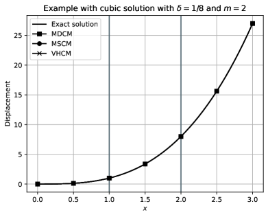
(a)

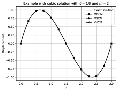
(b)

Figure 10: Examples with cubic manufactured solutions (63) and (64) for the problems (a) with mixed boundary conditions and (b) with Dirichlet boundary conditions at both extremities, respectively. The numerical solutions are shown here with horizon $\delta=1/8$ and grid size $h=\delta/m=1/16$.

6.2 Problems with quartic solutions

We consider in this section several problems whose manufactured solutions are given by polynomials of degree four. We know that the coupling methods will necessarily provide approximations with non-vanishing errors when compared to the solution to the classical elasticity problem. One difficulty in this case is to determine a measure to assess and compare the performance of the three coupling methods. In order to so, we propose to evaluate, for a given discretization $h$ of the domain, the difference $\Delta(x)$ between the discrete solution $u_{h,\text{CM}}$ of each coupling method and the finite difference solution $\underline{u}_{h,\text{FDM}}$ of the classical linear elasticity problem described in Section 2.1, that is

$$\Delta(x)=u_{h,\text{CM}}(x)-\underline{u}_{h,\text{FDM}}(x),\quad\forall x\in\overline{\Omega}.$$ (65)

We have seen in Section 3.2 that $\Delta(x)$ corresponds to an approximation of the function $v(x)$ (denoted $=v_{N}(x)$ in the case of mixed boundary conditions and $v_{D}(x)$ in the case of Dirichlet boundary conditions) satisfying Problem (16) that admits a maximal value $v_{\max}$ in $\overline{\Omega}$. We thus introduce in each case the error $\Delta_{\text{max}}$ as

$$\Delta_{\text{max}}=\max_{x\in\overline{\Omega}}\Delta(x),$$ (66)

and compute the relative error

$$\mathcal{E}_{r}=\bigg{|}\frac{\Delta_{\text{max}}-v_{\max}}{v_{\max}}\bigg{|}$$ (67)

in order to assess the quality of the discretized coupling methods. We note that the value of $v_{\max}$ depends on the exact solution $\underline{u}$ of the linear elasticity problem, on the type of boundary conditions, as well as on the profile of the horizon $\delta$ over the domain in terms of the interface locations $a$ and $b$.

In the examples below, we will treat both the $\delta$-convergence (see e.g. [33, 4]), for which $m$ is fixed while $\delta$ goes to zero, and the $m$-convergence, for which $\delta$ is fixed while $m$ increases, that is $h$ goes to zero.

6.2.1 Case with mixed boundary conditions

As before, we define the computational domain with $\ell=3$ and interface locations $a=1$ and $b=2$. We start with the simplest quartic manufactured solution, i.e. the monomial

$$\underline{u}(x)=x^{4}.$$ (68)

In the case of mixed boundary conditions, the data of the problem with $E=1$ are then given by

$$f_{b}(x)=-\underline{u}^{\prime\prime}(x)=-12x^{2},\qquad g=\underline{u}^{\prime}(\ell)=4\ell^{3}.$$ (69)

For MDCM and MSCM, the maximal value of $v_{N}(x)$ is attained for any point in the interval $[2,3]$ and is given by (20). For VHCM, the value needs to be corrected to take into account the fact that the horizon $\delta$ varies in the proximity of the interfaces. Omitting the lengthy calculations, one gets:

$$v_{N,\max}=\frac{\lambda\delta^{2}}{48}(b^{2}-a^{2})-\frac{\lambda}{36}(a+b)\delta^{3}=\frac{3}{2}\delta^{2}-2\delta^{3},$$ (70)

where it is reminded that $\lambda=\underline{u}^{\prime\prime\prime\prime}=24$ and $\delta$ corresponds to the constant provided in (26). Values of $v_{N,\max}$ for various horizons and for the three coupling methods are reported in Table 1. We also compile in this table the numerical values of $\Delta_{\text{max}}$ and $\mathcal{E}_{r}$ obtained by the three methods and several values of $\delta$ and $m$. Plots of the function $\Delta(x)$ are shown in Figure 11 for a corresponding subset of $\delta$ and $m$.

We observe from these results that the error $\Delta_{\text{max}}$ exhibits quadratic convergence with respect to the parameter $\delta$ for the three coupling methods, as expected, meaning that their solutions all converge to the classical linear elasticity solution as $\delta$ tends to zero. First, we see for $m=8$ that the errors $\Delta_{\text{max}}$ are all very close to the respective value of $v_{N,\text{max}}$ for the three approaches, even more so when $\delta$ is small. However, we would like to point out that the behavior of MDCM clearly differs from that of MSCM and VHCM in terms of $m$-convergence, and in particular for $\delta=1/8$, see for instance the right column of Figure 11. First, for $m=2$ and each value of $\delta$, we observe that the relative error $\mathcal{E}_{r}$ associated with MDCM is consistently larger than that obtained by the other two methods. We also see that $\mathcal{E}_{r}$ is larger for MDCM than for MSCM for $m=4$ when $\delta=1/16$, $1/32$, and $1/64$. In the case $m=4$ and $\delta=1/8$, the relative error for MDCM is coincidentally much smaller than that for MSCM, but increases again a lot when $m$ is increased to $8$ due to the fact that $\Delta_{\text{max}}$ now overshoots $v_{N,\text{max}}$. In fact, we regularly observe larger variations in $\Delta_{\text{max}}$ for MDMC when the value of $m$ is increased. On the other hand, the behaviors of the MSCM and VHCM solutions are similar. For these reasons, the latter two methods seem to exhibit a more stable behavior for the coupling of peridynamic and classical linear elasticity models.

		Error $\Delta_{\text{max}}$			Relative error $\mathcal{E}_{r}$
$\delta$	$m$	MDCM	MSCM	VHCM	MDCM	MSCM	VHCM
$\nicefrac{{1}}{{8}}$	2	$0.018{}998{}5$	$0.026{}689{}0$	$0.022{}535{}0$	$0.189{}395{}630{}363{}530{}16$	$0.138{}729{}369{}657{}994{}54$	$0.153{}791{}260{}758{}771{}4$
	4	$0.023{}442{}7$	$0.025{}228{}0$	$0.019{}469{}5$	$0.000{}223{}196{}278{}360{}167{}84$	$0.076{}395{}071{}273{}206{}37$	$0.003{}163{}265{}463{}081{}188{}6$
	8	$0.024{}505{}7$	$0.025{}003{}5$	$0.019{}591{}7$	$0.045{}576{}525{}052{}941{}484$	$0.066{}816{}759{}477{}357{}37$	$0.003{}092{}732{}426{}011{}935$
$v_{N,\max}$		$0.023{}437{}5$	$0.023{}437{}5$	$0.019{}531{}2$
$\nicefrac{{1}}{{16}}$	2	$0.004{}572{}1$	$0.005{}533{}4$	$0.005{}014{}1$	$0.219{}697{}814{}575{}435{}27$	$0.055{}635{}314{}542{}693{}47$	$0.066{}458{}517{}121{}976{}58$
	4	$0.005{}676{}9$	$0.005{}900{}1$	$0.005{}180{}3$	$0.031{}138{}402{}603{}877{}086$	$0.006{}947{}535{}851{}698{}679$	$0.035{}528{}756{}926{}809{}86$
	8	$0.005{}947{}1$	$0.006{}009{}4$	$0.005{}332{}9$	$0.014{}975{}760{}039{}912{}226$	$0.025{}595{}878{}730{}503{}802$	$0.007{}116{}942{}243{}142{}562$
$v_{N,\max}$		$0.005{}859{}4$	$0.005{}859{}4$	$0.005{}371{}1$
$\nicefrac{{1}}{{32}}$	2	$0.001{}120{}8$	$0.001{}241{}0$	$0.001{}176{}1$	$0.234{}848{}905{}713{}685{}47$	$0.152{}817{}655{}063{}699{}93$	$0.162{}219{}288{}607{}087{}48$
	4	$0.001{}396{}3$	$0.001{}424{}2$	$0.001{}334{}2$	$0.046{}819{}206{}108{}921{}21$	$0.027{}776{}237{}957{}975{}052$	$0.049{}600{}713{}886{}320{}59$
	8	$0.001{}464{}4$	$0.001{}472{}1$	$0.001{}387{}6$	$0.000{}324{}586{}935{}069{}722{}4$	$0.004{}985{}458{}886{}949{}345{}5$	$0.011{}555{}923{}639{}958{}643$
$v_{N,\max}$		$0.001{}464{}8$	$0.001{}464{}8$	$0.001{}403{}8$
$\nicefrac{{1}}{{64}}$	2	$0.000{}277{}4$	$0.000{}292{}5$	$0.000{}284{}3$	$0.242{}424{}423{}350{}409{}28$	$0.201{}408{}801{}600{}337{}03$	$0.207{}043{}454{}922{}894{}22$
	4	$0.000{}346{}2$	$0.000{}349{}7$	$0.000{}338{}4$	$0.054{}659{}935{}083{}085{}05$	$0.045{}138{}084{}931{}143{}87$	$0.056{}187{}605{}980{}704{}44$
	8	$0.000{}363{}3$	$0.000{}364{}3$	$0.000{}292{}5$	$0.007{}974{}629{}979{}192{}59$	$0.005{}320{}158{}602{}747{}445$	$0.013{}634{}200{}316{}873{}636$
$v_{N,\max}$		$0.000{}366{}2$	$0.000{}366{}2$	$0.000{}358{}6$

Table 1: Error $\Delta_{\text{max}}$ and relative error $\mathcal{E}_{r}$ with respect to parameters $\delta$ and $m$ obtained by the three coupling methods in the case of the quartic solution for the problem with mixed boundary conditions and interface locations $a=1$ and $b=2$.

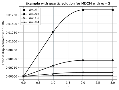
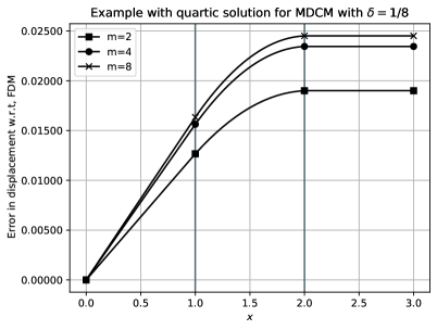
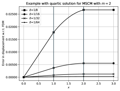
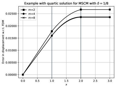
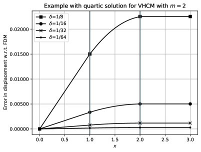
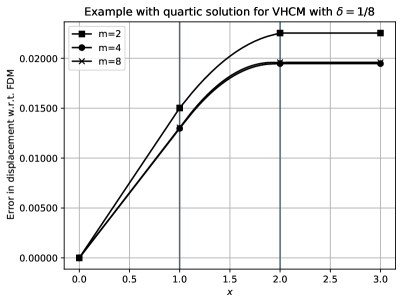
Figure 11: Error $\Delta(x)$ obtained by the three coupling methods (top row: MDCM, middle row: MSCM, and bottow row: VHCM) in the case of the quartic solution for the problem with mixed boundary conditions and interface locations $a=1$ and $b=2$. Left column: $\delta$-convergence with $m=2$. Right column: $m$-convergence with $\delta=1/8$.

6.2.2 Case with Dirichlet boundary conditions at both extremities

We first consider a symmetric problem with a symmetric quartic solution with respect to $x=3/2$. The computational domain is kept as $\Omega=(0,3)$ with interfaces located at $a=1$ and $b=2$. The manufactured displacement field is chosen as

$$\underline{u}(x)=\frac{16}{81}\ x^{2}(3-x)^{2}=\frac{16}{9}x^{2}-\frac{32}{27}x^{3}+\frac{16}{81}x^{4},$$ (71)

such that the corresponding load is given by

$$f_{b}(x)=-\underline{u}^{\prime\prime}(x)=-\frac{32}{9}+\frac{64}{9}x-\frac{64}{27}x^{2}.$$ (72)

Moreover, we solved the problem with homogeneous Dirichlet boundary conditions at both extremities $x=0$ and $x=\ell=3$. For MDCM and MSCM, the maximal value of $v_{D}(x)$ is in this case achieved at $x=3/2$ due to the symmetry of the problem and is given by (21). For VHCM, this value is modified as follows:

$$v_{D,\max}=\frac{\lambda\delta^{2}}{48}(b^{2}-a^{2})\frac{4\ell^{2}-4b\ell+b^{2}-a^{2}}{4\ell^{2}}-\frac{\lambda\delta^{3}}{48}\frac{8a+3\delta}{6}=\frac{10}{81}\delta^{2}-\frac{4}{243}\delta^{3}(8+3\delta),$$ (73)

where $\lambda=\underline{u}^{\prime\prime\prime\prime}=128/27$. The quantity $v_{D,\max}$, as well as the numerical values of $\Delta_{\text{max}}$ and $\mathcal{E}_{r}$, are provided in Table 2 for several values of $\delta$ and $m$. Moreover, we show in Figure 12 some plots of $\Delta(x)$ to illustrate the $\delta$-convergence and $m$-convergence of the coupling approaches. We first observe that all functions $\Delta(x)$ are symmetric with respect to $x=3/2$, as expected. Moreover, the conclusions from the previous example all pertain in this case.

We now repeat the same exercise in the case of an asymmetric problem by moving the first interface to $a=3/4$ while keeping the second interface located at $b=2$. We again solve the problem with homogeneous Dirichlet boundary conditions at both ends defined such that it is satisfied by the manufactured solution (71). The values of $v_{D,\max}$ for this new configuration are computed from their analytic expressions and shown in Table 3. The expressions for $v_{D,\max}$ are omitted here due to their complexity, but the maximal value is attained for MDCM and MSCM at:

$$x_{D,\max}=\frac{2b\ell+a^{2}-b^{2}}{2\ell}\frac{137}{96}\approx 1.427,$$ (74)

and for VHCM at:

$$x_{D,\max}=\frac{2b\ell+a^{2}-b^{2}}{2\ell}+2\delta\frac{a+b-\ell}{3\ell}=\frac{137}{96}-\frac{\delta}{18}\approx 1.427-0.056\times\delta.$$ (75)

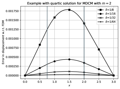
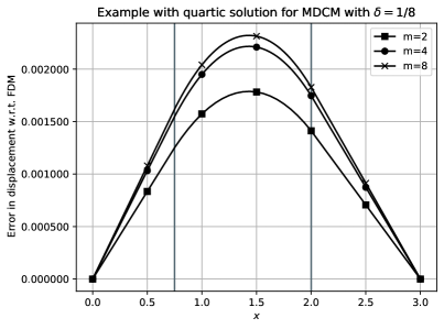
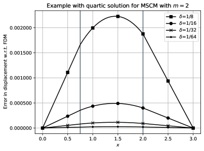
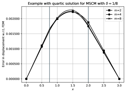
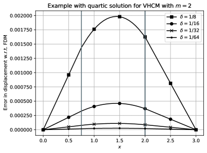
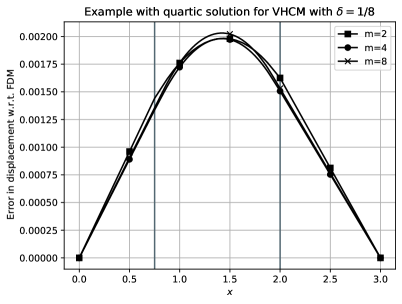
Figure 13: Error $\Delta(x)$ obtained by the three coupling methods (top row: MDCM, middle row: MSCM, and bottom row: VHCM) in the case of the quartic solution for the problem with Dirichlet boundary conditions at both extremities and interface locations $a=3/4$ and $b=2$. Left column: $\delta$-convergence with $m=2$. Right column: $m$-convergence with $\delta=1/8$.

The numerical results for $\Delta_{\text{max}}$ and $\mathcal{E}_{r}$ are reported in Table 3 and plots of the function $\Delta(x)$ are shown in Figure 13. We observe that the three coupling methods still exhibit a quadratic convergence with respect to the parameter $\delta$ and that the relative errors are similar to the previous case. However, we note that in the case $\delta=1/8$, see right column of Figure 3, the function $\Delta(x)$ for MSCM and VHCM does not change much and its maximal value remains close to $v_{D,\max}$ as $m$ is increased, unlike for MDCM. In other words, the two coupling methods are less sensitive to the mesh size $h$ for a given value of $\delta$.

		Error $\Delta_{\text{max}}$			Relative error $\mathcal{E}_{r}$
$\delta$	$m$	MDCM	MSCM	VHCM	MDCM	MSCM	VHCM
$\nicefrac{{1}}{{8}}$	2	$0.001{}540{}090{}595{}820{}276$	$0.002{}047{}2$	$0.001{}766{}549{}160{}763{}242{}2$	$0.201{}617{}035{}126{}768{}9$	$0.061{}270{}253{}688{}333{}36$	$0.064{}343{}730{}680{}482{}09$
	4	$0.001{}904{}861{}362{}222{}343{}1$	$0.002{}022{}6$	$0.001{}634{}976{}790{}774{}178{}6$	$0.012{}493{}519{}958$	$0.048{}500{}436{}653{}854{}76$	$0.014{}928{}462{}949{}345{}231$
	8	$0.001{}992{}916{}576{}625{}036{}7$	$0.002{}025{}8$	$0.001{}660{}535{}142{}109{}509{}4$	$0.033{}127{}953{}322{}419{}1$	$0.050{}165{}508{}954{}386{}04$	$0.000{}470{}412{}787{}877{}609{}9$
$v_{D,\max}$		$0.001{}929{}012{}346$	$0.001{}929{}012{}346$	$0.001{}659{}754{}372$
$\nicefrac{{1}}{{16}}$	2	$0.000{}373{}368{}352{}221{}348{}23$	$0.000{}436{}7$	$0.000{}402{}075{}286{}197{}289{}83$	$0.225{}783{}384{}833{}812{}27$	$0.094{}436{}562{}448{}430{}5$	$0.105{}205{}611{}044{}882{}88$
	4	$0.000{}464{}187{}726{}735{}954$	$0.000{}478{}9$	$0.000{}430{}969{}062{}419{}350{}73$	$0.037{}460{}329{}840{}325{}76$	$0.006{}970{}876{}479{}976{}996$	$0.040{}904{}248{}273{}387{}206$
	8	$0.000{}486{}498{}620{}055{}897{}4$	$0.000{}490{}6$	$0.000{}445{}502{}375{}741{}035{}9$	$0.008{}803{}538{}547{}908{}885$	$0.017{}310{}979{}031{}270{}848$	$0.008{}561{}232{}774{}569{}41$
$v_{D,\max}$		$0.000{}482{}253{}086$	$0.000{}482{}253{}086$	$0.000{}449{}349{}360$
$\nicefrac{{1}}{{32}}$	2	$0.000{}091{}9$	$0.000{}099{}8$	$0.000{}095{}5$	$0.237{}885{}407{}181{}670{}37$	$0.172{}236{}201{}861{}255{}68$	$0.180{}270{}370{}019{}641{}7$
	4	$0.000{}114{}538{}994{}865{}576{}17$	$0.000{}116{}4$	$0.000{}110{}4$	$0.049{}967{}760{}986{}964{}954$	$0.034{}728{}212{}000{}686$	$0.052{}176{}552{}823{}624{}89$
	8	$0.000{}120{}153{}645{}565{}279{}63$	$0.000{}120{}7$	$0.000{}115{}1$	$0.003{}397{}602{}223{}344{}564{}6$	$0.000{}853{}173{}054{}179{}079{}4$	$0.012{}307{}868{}862{}550{}942$
$v_{D,\max}$		$0.000{}120{}563{}272$	$0.000{}120{}563{}272$	$0.000{}116{}497{}401$
$\nicefrac{{1}}{{64}}$	2	$0.000{}022{}8$	$0.000{}023{}8$	$0.000{}023{}2$	$0.243{}941{}059{}771{}350{}36$	$0.211{}122{}557{}184{}626{}16$	$0.215{}756{}749{}211{}533{}15$
	4	$0.000{}028{}4$	$0.000{}028{}7$	$0.000{}027{}9$	$0.056{}232{}371{}164{}696{}76$	$0.048{}612{}301{}320{}281{}354$	$0.057{}449{}163{}616{}189{}465$
	8	$0.000{}029{}9$	$0.000{}029{}9$	$0.000{}029{}2$	$0.009{}505{}537{}756{}285{}721$	$0.007{}383{}440{}771{}263{}794$	$0.014{}016{}858{}778{}185{}955$
$v_{D,\max}$		$0.000{}030{}140{}818$	$0.000{}030{}140{}818$	$0.000{}029{}635{}527$

Table 2: Error $\Delta_{\text{max}}$ and relative error $\mathcal{E}_{r}$ with respect to parameters $\delta$ and $m$ obtained by the three coupling methods in the case of the quartic solution for the problem with Dirichlet boundary conditions at both extremities and interface locations $a=1$ and $b=2$.

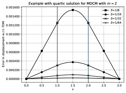
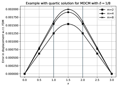
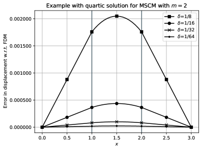
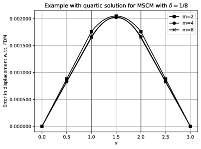
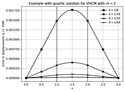
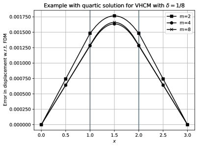
Figure 12: Error $\Delta(x)$ obtained by the three coupling methods (top row: MDCM, middle row: MSCM, and bottow row: VHCM) in the case of the quartic solution for the problem with Dirichlet boundary conditions at both extremities and interface locations $a=1$ and $b=2$. Left column: $\delta$-convergence with $m=2$. Right column: $m$-convergence with $\delta=1/8$.

		Error $\Delta_{\text{max}}$			Relative error $\mathcal{E}_{r}$
$\delta$	$m$	MDCM	MSCM	VHCM	MDCM	MSCM	VHCM
$\nicefrac{{1}}{{8}}$	2	$0.001{}787{}1$	$0.002{}228{}3$	$0.001{}983{}3$	$0.214{}381{}984{}779{}283{}05$	$0.020{}439{}753{}512{}364{}74$	$0.027{}478{}500{}421{}319{}264$
	4	$0.002{}216{}3$	$0.002{}240{}9$	$0.001{}980{}5$	$0.025{}729{}017{}096{}367{}362$	$0.014{}897{}390{}530{}104{}738$	$0.028{}857{}258{}758{}598{}95$
	8	$0.002{}320{}8$	$0.002{}288{}6$	$0.002{}031{}0$	$0.020{}236{}480{}491{}349{}07$	$0.006{}087{}077{}080{}257{}216$	$0.004{}068{}147{}175{}928{}762$
$v_{D,\max}$		$0.002{}274{}794{}507$	$0.002{}274{}794{}507$	$0.002{}039{}324{}018$
$\nicefrac{{1}}{{16}}$	2	$0.000{}436{}6$	$0.000{}491{}7$	$0.000{}461{}6$	$0.232{}198{}189{}445{}919{}3$	$0.135{}309{}178{}403{}936{}6$	$0.145{}248{}317{}629{}815{}7$
	4	$0.000{}543{}6$	$0.000{}546{}6$	$0.000{}514{}7$	$0.044{}084{}026{}844{}382{}736$	$0.038{}786{}377{}562{}855{}24$	$0.046{}830{}792{}425{}876{}885$
	8	$0.000{}570{}0$	$0.000{}565{}9$	$0.000{}534{}4$	$0.002{}366{}745{}633{}618{}890{}4$	$0.004{}869{}687{}299{}632{}944$	$0.010{}456{}991{}628{}599{}597$
$v_{D,\max}$		$0.000{}568{}698{}627$	$0.000{}568{}698{}627$	$0.000{}540{}013{}685$
$\nicefrac{{1}}{{32}}$	2	$0.000{}107{}9$	$0.000{}114{}8$	$0.000{}111{}0$	$0.241{}227{}677{}712{}863{}74$	$0.192{}840{}225{}710{}174{}26$	$0.198{}895{}787{}355{}704{}6$
	4	$0.000{}134{}6$	$0.000{}135{}0$	$0.000{}131{}0$	$0.053{}437{}798{}819{}612{}92$	$0.050{}840{}163{}803{}476{}33$	$0.054{}718{}399{}047{}896{}2$
	8	$0.000{}141{}2$	$0.000{}140{}7$	$0.000{}136{}8$	$0.006{}796{}241{}671{}615{}282$	$0.010{}451{}276{}475{}890{}435$	$0.012{}938{}404{}917{}037{}115$
$v_{D,\max}$		$0.000{}142{}174{}657$	$0.000{}142{}174{}657$	$0.000{}138{}635{}843$
$\nicefrac{{1}}{{64}}$	2	$0.000{}026{}8$	$0.000{}027{}7$	$0.000{}027{}2$	$0.244{}610{}129{}511{}041{}47$	$0.220{}391{}545{}355{}693{}8$	$0.224{}784{}696{}049{}617{}34$
	4	$0.000{}033{}5$	$0.000{}033{}5$	$0.000{}033{}0$	$0.056{}725{}458{}709{}944{}04$	$0.055{}430{}665{}895{}507{}21$	$0.058{}679{}439{}953{}514{}54$
	8	$0.000{}035{}1$	$0.000{}035{}1$	$0.000{}034{}6$	$0.009{}900{}291{}732{}917{}996$	$0.011{}742{}162{}479{}606{}442$	$0.014{}324{}200{}994{}094{}661$
$v_{D,\max}$		$0.000{}035{}543{}664$	$0.000{}035{}543{}664$	$0.000{}035{}104{}238$

Table 3: Error $\Delta_{\text{max}}$ and relative error $\mathcal{E}_{r}$ with respect to parameters $\delta$ and $m$ obtained by the three coupling methods in the case of the quartic solution for the problem with Dirichlet boundary conditions at both extremities and interface locations $a=3/4$ and $b=2$.

6.3 Influence of the peridynamic material parameter

We have seen from the last examples that the coupling methods cannot reproduce quartic solutions (or solutions that involve polynomials of degree at least four) to the classical linear elasticity model in the case of finite values of the horizon $\delta$, even if the mesh size $h$ goes to zero, due to the fact that the choice of the material parameter, i.e. $\kappa=2E/\delta^{2}$, provides a perfectly compatible peridynamic model only in the limit when $\delta$ vanishes. This theoretical result is certainly well known within the peridynamics community. However, we emphasize this point again as it does influence the construction and performance of the coupling approaches.

We observe in Figures 11, 12, and 13 that the error $\Delta(x)$ remains small in all cases when compared to the solution $\underline{u}(x)$, in the sense that it approximates the modeling error $v(x)$, which can be shown to be of the order $E\underline{u}^{\prime\prime\prime\prime}\delta^{2}/24$, see Eq. (16). The challenge here is whether one could identify a value of $\kappa$ that decreases the modeling error. In fact, it is well known that it is not possible to find a value that would allow one to exactly match the solution to the classical linear elasticity model as the material parameter would need in that case to depend on $x$. We nevertheless test several values of the parameter, chosen as corrections of order $\delta^{2}$ of the nominal value $\kappa=2E/\delta^{2}$. We take here $m=2$ and $\delta=1/8$, so that the nominal value is given by $\kappa=128$. We consider the usual configuration with $\ell=3$ and interface locations $a=1$ and $b=2$. We show in Figure 14 the error $\Delta(x)$ associated with the quartic solutions to the problems with mixed boundary conditions and with Dirichlet boundary conditions using MDCM and MSCM for several values of $\kappa$, including the nominal value. The main conclusion is that it is indeed possible to find a value of the parameter for which the error is overall much smaller than that with the nominal value. However, we also observe that the best value of $\kappa$ is very much dependent on the solution itself and the coupling method used. Moreover, the error is quite sensitive to the value of $\kappa$.

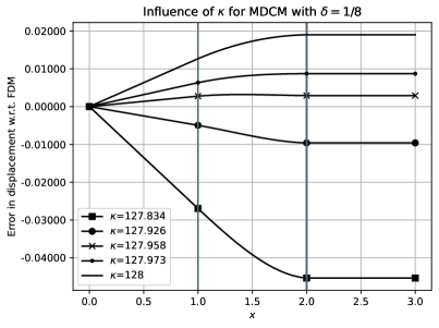
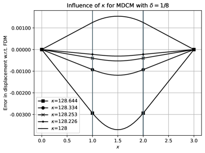
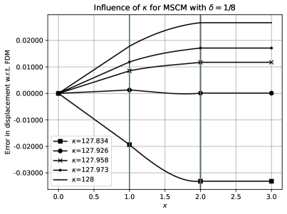
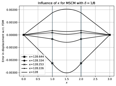
Figure 14: Influence of material parameter $\kappa$ on the error function $\Delta(x)$ for the coupling methods MDCM (top row) and MSCM (bottom row) in the case of the quartic solutions for the problem with mixed boundary conditions (left) and for the problem with Dirichlet boundary conditions at both extremities (right). The parameters of the simulations are $m=2$, $\delta=1/8$, $a=1$, $b=2$, and $\ell=3$.

6.4 Condition number of the coupled systems

We analyze in this section the condition number of the stiffness matrices $M$ resulting from the coupling methods. We used the Numpy function numpy.linalg.con to compute the condition number $\text{Cond}(M)$ for each coupling approach. The condition number is computed here with respect to the $\ell^{2}$-norm as $\text{Cond}(M)={\|M\|_{\ell_{2}}}{\|M^{-1}\|_{\ell_{2}}}$ [18]. Figure 15 shows the results for the two problems considered earlier, namely the problem with mixed boundary conditions and that with homogeneous Dirichlet boundary conditions. The only difference between the two problems lies in the last row of the matrix, which implements either the Neumann or Dirichlet boundary condition. We observe that, for both problems, the condition number associated with MDCM is larger than the ones obtained for MSCM, VHCM, or the Finite Difference Method (FDM) applied to (1). For small values of $\delta$, the condition number can be two orders of magnitude or more. From a numerical point of view, systems of equations with lower condition numbers should be favored.

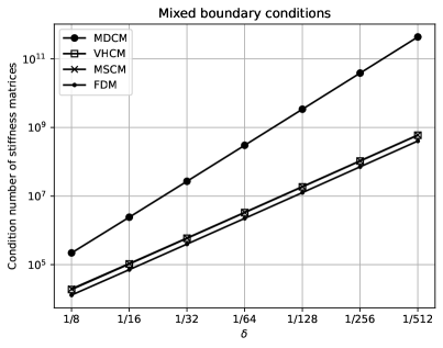
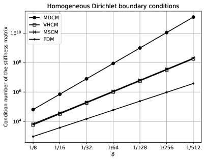
Figure 15: Condition number of the stiffness matrices with respect to the horizon $\delta$ for the problem with mixed boundary conditions (left) and the problem with homogeneous Dirichlet boundary conditions (right).

7 Conclusions

We have presented and compared in this paper three methods, namely the coupling method with matching displacements (MDCM), the coupling method with matching stresses (MSCM), and the variable horizon coupling method (VHCM), for coupling classical linear elasticity and peridynamic models. The methods were developed based on the general coupling formulation of classical linear elasticity models. We have provided the continuous formulations of the three corresponding problems and their corresponding discrete formulations using for instance the classical finite difference method. One challenge in comparing the three methods was to determine an adequate measure to assess the performance of each method. We have proposed to evaluate the maximum value of the difference between the solution of each coupling method and the solution to the classical linear elasticity problem. This difference actually corresponds to the modeling error between the two models.

We have shown on one-dimensional examples with cubic solutions that the three methods were able to recover the exact solution of the classical linear elasticity problem as predicted by the theory. It follows that the interesting numerical test cases for the purpose of comparison are those that involve polynomial functions of degree at least four. We have therefore considered several one-dimensional examples whose manufactured solutions were defined in terms of quartic polynomial functions. The $\delta$- and $m$-convergence results have shown that the three coupling methods provide comparable errors when $\delta$ tends to zero, i.e. when the modeling error between the classical linear elasticity and peridynamic models become very small. However, the results show that the matching stress approach (MSCM) is less sensitive to the mesh size than the matching displacement approach (MDCM) whenever the value of the horizon parameter is not so small. This is an important result as most coupling approaches from the literature constrain the displacement fields to match in the coupling region. We have also observed that VHCM usually exhibits a similar behavior as MSCM. The original feature of VHCM is that, unlike the other two methods, it avoids introducing an overlap region between the two models. Moreover, we have indicated for finite values of the horizon $\delta$ that it was possible to reduce the modeling error by considering corrections in parameter $\delta$ of the order of $\delta^{2}$.

The interfaces between the classical linear elasticity and peridynamic models in a coupling strategy should be preferably located in the regions where the solution to the problem has a local behavior. These regions can often be identified a priori in the case of steady-state problems but this could become trickier when considering dynamical systems. In this case, one should choose a coupling approach that generates the smallest errors in order to avoid wave reflection phenomena at the interfaces. One could also appeal to error estimation and adaptivity to automatically determine the regions where the two models should be coupled, see e.g. [29, 1, 2]. This is left for future work. One also notes that MSCM could be used as an alternative candidate for the application of boundary conditions in peridynamic problems to those presented in [30]. Nevertheless, this is a preliminary study of coupling methods and additional work needs to be carried out to confirm the performance of the three methods in more general situations. The performance of the coupling approaches should be assessed, for instance, when using other discretization methods, such as the finite element method, for their implementation. The methods should also be extended to two- and three-dimensional problems and to the case of state-based peridynamic modeling.

Supplementary materials

The Python code (using numpy [25, 40] and matplotlib [16]) used to generate the numerical results is available on GitHub^® and on Zenodo^® [10].

Conflict of interest

The authors declare that they have no conflict of interest.

References

- [1] Paul T. Bauman, J. Tinsley Oden, and Serge Prudhomme. Adaptive multiscale modeling of polymeric materials: Arlequin coupling and goals algorithms. Computer Methods in Applied Mechanics and Engineering, 198:799–818, 2009.
- [2] Hachmi Ben Dhia, Ludovic Chamoin, J. Tinsley Oden, and Serge Prudhomme. An adaptive strategy for the control of modeling error in two-dimensional atomic-to-continuum coupling simulations. Computer Methods in Applied Mechanics and Engineering, 200:2675–2696, 2011.
- [3] YH Bie, XY Cui, and ZC Li. A coupling approach of state-based peridynamics with node-based smoothed finite element method. Computer Methods in Applied Mechanics and Engineering, 331:675–700, 2018.
- [4] Florin Bobaru, Mijia Yabg, Leonardo F. Alves, Stewart A. Silling, Ebrahim Askari, and Jifeng Xu. Convergence, adaptive refinement, and scaling in 1D peridynamics. International Journal for Numerical Methods in Engineering, 77:852–877, 2009.
- [5] Marta D’Elia and Pavel Bochev. Formulation, analysis and computation of an optimization-based local-to-nonlocal coupling method. Results in Applied Mathematics, 9:100129, 2021.
- [6] Marta D’Elia, Xingjie Li, Pablo Seleson, Xiaochuan Tian, and Yue Yu. A review of local-to-nonlocal coupling methods in nonlocal diffusion and nonlocal mechanics. Journal of Peridynamics and Nonlocal Modeling, 2021.
- [7] Marta D’Elia, Xiaochuan Tian, and Yue Yu. A physically consistent, flexible, and efficient strategy to convert local boundary conditions into nonlocal volume constraints. SIAM Journal on Scientific Computing, 42(4):A1935–A1949, 2020.
- [8] Marta D’Elia and Yue Yu. On the prescription of boundary conditions for nonlocal poisson’s and peridynamics models. arXiv preprint arXiv:2107.04450, 2021.
- [9] Patrick Diehl, Robert Lipton, Thomas Wick, and Mayank Tyagi. A comparative review of peridynamics and phase-field models for engineering fracture mechanics, 2021. Submitted.
- [10] Patrick Diehl and Serge Prudhomme. Supplementary materials: Coupling approaches for classical linear elasticity and bond-based peridynamic models, May 2021.
- [11] Patrick Diehl, Serge Prudhomme, and Martin Lévesque. A review of benchmark experiments for the validation of peridynamics models. Journal of Peridynamics and Nonlocal Modeling, 1(1):14–35, Apr 2019.
- [12] Qiang Du. Nonlocal calculus of variations and well-posedness of peridynamics. In Handbook of Peridynamic Modeling, pages 101–124. Chapman and Hall/CRC, 2016.
- [13] Guodong Fang, Shuo Liu, Maoqing Fu, Bing Wang, Zengwen Wu, and Jun Liang. A method to couple state-based peridynamics and finite element method for crack propagation problem. Mechanics Research Communications, 95:89–95, 2019.
- [14] Ugo Galvanetto, Teo Mudric, Arman Shojaei, and Mirco Zaccariotto. An effective way to couple FEM meshes and peridynamics grids for the solution of static equilibrium problems. Mechanics Research Communications, 76:41–47, 2016.
- [15] Xin Gu, Erdogan Madenci, and Qing Zhang. Revisit of non-ordinary state-based peridynamics. Engineering Fracture Mechanics, 190:31–52, 2018.
- [16] J. D. Hunter. Matplotlib: A 2d graphics environment. Computing in Science & Engineering, 9(3):90–95, 2007.
- [17] Bahattin Kilic and Erdogan Madenci. Coupling of peridynamic theory and the finite element method. Journal of Mechanics of Materials and Structures, 5(5):707–733, 2010.
- [18] David C Lay, Steven R Lay, and Judi J McDonald. Linear algebra and its applications. Pearson, 2016.
- [19] Wenyang Liu and Jung-Wuk Hong. A coupling approach of discretized peridynamics with finite element method. Computer Methods in Applied Mechanics and Engineering, 245:163–175, 2012.
- [20] Erdogan Madenci, Atila Barut, Mehmet Dorduncu, and Nam D Phan. Coupling of peridynamics with finite elements without an overlap zone. In 2018 AIAA/ASCE/AHS/ASC Structures, Structural Dynamics, and Materials Conference, page 1462, 2018.
- [21] Erdogan Madenci, Mehmet Dorduncu, Atila Barut, and Nam Phan. A state-based peridynamic analysis in a finite element framework. Engineering Fracture Mechanics, 195:104–128, 2018.
- [22] Erdogan Madenci, Mehmet Dorduncu, Atila Barut, and Nam Phan. Weak form of peridynamics for nonlocal essential and natural boundary conditions. Computer Methods in Applied Mechanics and Engineering, 337:598–631, 2018.
- [23] Tao Ni, Mirco Zaccariotto, Qi-Zhi Zhu, and Ugo Galvanetto. Coupling of FEM and ordinary state-based peridynamics for brittle failure analysis in 3D. Mechanics of Advanced Materials and Structures, 28(9):875–890, 2021.
- [24] Jaber Nikpayam and Mohammad Ali Kouchakzadeh. A variable horizon method for coupling meshfree peridynamics to FEM. Computer Methods in Applied Mechanics and Engineering, 355:308–322, 2019.
- [25] Travis E Oliphant. A guide to NumPy, volume 1. Trelgol Publishing USA, 2006.
- [26] Greta Ongaro, Pablo Seleson, Ugo Galvanetto, Tao Ni, and Mirco Zaccariotto. Overall equilibrium in the coupling of peridynamics and classical continuum mechanics. Computer Methods in Applied Mechanics and Engineering, 381:113515, 2021.
- [27] Michael L Parks, Richard B Lehoucq, Steven J Plimpton, and Stewart A Silling. Implementing peridynamics within a molecular dynamics code. Computer Physics Communications, 179(11):777–783, 2008.
- [28] Michael L. Parks, Richard B. Lehoucq, Steven J. Plimpton, and Stewart A. Silling. Implementing peridynamics within a molecular dynamics code. Computer Physics Communications, 179(11):777–783, 2008.
- [29] Serge Prudhomme, Ludovic Chamoin, Hachmi Ben Dhia, and Paul T. Bauman. An adaptive strategy for the control of modeling error in two-dimensional atomic-to-continuum coupling simulations. Computer Methods in Applied Mechanics and Engineering, 198:1887–1901, 2009.
- [30] Serge Prudhomme and Patrick Diehl. On the treatment of boundary conditions for bond-based peridynamic models. Computer Methods in Applied Mechanics and Engineering, 372:113391, 2020.
- [31] Pablo Seleson. Improved one-point quadrature algorithms for two-dimensional peridynamic models based on analytical calculations. Computer Methods in Applied Mechanics and Engineering, 282:184–217, 2014.
- [32] Pablo Seleson, Qiang Du, and Michael L. Parks. On the consistency between nearest-neighbor peridynamic discretizations and discretized classical elasticity models. Computer Methods in Applied Mechanics and Engineering, 311:698–722, 2016.
- [33] Pablo Seleson and David J Littlewood. Convergence studies in meshfree peridynamic simulations. Computers & Mathematics with Applications, 71(11):2432–2448, 2016.
- [34] SA Silling. Local-nonlocal coupling in Emu/PDMS. Sandia Report (SAND2020-11382), 2020.
- [35] Stewart Silling, David Littlewood, and Pablo Seleson. Variable horizon in a peridynamic medium. Journal of Mechanics of Materials and Structures, 10(5):591–612, 2015.
- [36] Stewart A. Silling. Reformulation of elasticity theory for discontinuities and long-range forces. Journal of the Mechanics and Physics of Solids, 48:175–209, 2000.
- [37] Stewart A. Silling and Ebrahim Askari. A meshfree method based on the peridynamic model of solid mechanics. Computers & Structures, 83(17-18):1526–1535, 2005.
- [38] Wei Sun and Jacob Fish. Superposition-based coupling of peridynamics and finite element method. Computational Mechanics, 64:231–248, 2019.
- [39] Nathaniel Trask, Huaiqian You, Yue Yu, and Michael L. Parks. An asymptotically compatible meshfree quadrature rule for nonlocal problems with applications to peridynamics. Computer Methods in Applied Mechanics and Engineering, 343:151–165, 2019.
- [40] S. van der Walt, S. C. Colbert, and G. Varoquaux. The NumPy Array: A structure for efficient numerical computation. Computing in Science & Engineering, 13(2):22–30, 2011.
- [41] Huaiqian You, XinYang Lu, Nathaniel Task, and Yue Yu. An asymptotically compatible approach for neumann-type boundary condition on nonlocal problems. ESAIM: Mathematical Modelling and Numerical Analysis, 54(4):1373–1413, 2020.
- [42] Mirco Zaccariotto, Teo Mudric, Davide Tomasi, Arman Shojaei, and Ugo Galvanetto. Coupling of FEM meshes with Peridynamic grids. Computer Methods in Applied Mechanics and Engineering, 330:471–497, 2018.
- [43] Mirco Zaccariotto, Davide Tomasi, and Ugo Galvanetto. An enhanced coupling of PD grids to FE meshes. Mechanics Research Communications, 84:125–135, 2017.