Abstract. The sample average approximation (SAA) and the stochastic approximation (SA) are two popular schemes for solving the stochastic variational inequalities problem (SVIP). In the past decades, theories on the consistency of the SAA solutions and SA solutions have been well studied. More recently, the asymptotic confidence regions of the true solution to SVIP have been constructed when the SAA scheme is implemented. It is of fundamental interest to develop confidence regions of the true solution to the SVIP when the SA scheme is employed. In this paper, we discuss the framework of constructing asymptotic confidence regions for the true solution of SVIP with a focus on stochastic dual average method. We first establish the asymptotic normality of the SA solutions both in ergodic sense and non-ergodic sense. Then the online methods of estimating the covariance matrices in the normal distributions are studied. Finally, practical procedures of building the asymptotic confidence regions of solutions to SVIP with numerical simulations are presented.

Key words. Stochastic variational inequalities, confidence regions, stochastic approximation, statistical inference

1 Introduction

For the given convex set ${\cal C}\subset{\rm I\!R}^{n}$ and a mapping $f:{\cal C}\rightarrow{\rm I\!R}^{n}$, the variational inequalities problem (VIP) is to find a vector $x\in{\cal C}$ such that

$$(y-x)^{T}f(x)\geq 0,\quad\forall y\in{\cal C}.$$

VIP has many applications in engineering, economics, game theory and has been well studied in theories, algorithms, see the monograph by Facchinei and Pang [1]. In order to describe decision making problems which involve future uncertainty, the stochastic version of variational inequalities problem (SVIP) has been proposed. Different approaches to incorporate the uncertainty into VIP induce different SVIP models, such as, expected residual minimization-SVIP (ERM-SVIP) model [2], expected value-SVIP (EV-SVIP) [3], $\mathcal{L}^{p}$-SVIP model [4], two-stage SVIP model [5] and multi-stage SVIP model [6].

In this paper, we focus on the EV-SVIP model (for simplicity, we refer the EV-SVIP as SVIP): find $x\in{\cal C}$ such that

$$(y-x)^{T}f(x)\geq 0,\quad\forall y\in{\cal C},$$ (1.1)

where $f(x):={\mathbb{E}}_{P}[F(x,\xi)]$, ${\cal C}\subset{\rm I\!R}^{n}$ is a convex set, $\xi$ is a random vector defined on probability space $(\Omega,\mathscr{F},P)$ with support set $\Xi$, $F(\cdot,\cdot)$ is measurable function from ${\cal C}\times\Xi$ to ${\rm I\!R}^{n}$ and ${\mathbb{E}}_{P}[\cdot]$ denotes the expected value with respect to the distribution $P$. Indeed, (1.1) is deterministic VIP if ${\mathbb{E}}_{P}[F(x,\xi)]$ has a closed form representation. However, in most problems of interest obtaining a closed form of ${\mathbb{E}}_{P}[\cdot]$ or computing its value numerically is usually difficult either due to the unavailability of distribution of $\xi$ or multiple integration involved. In general, it is more realistic to obtain a sample of the random vector $\xi$ either from past data or from computer simulation. Depending on how sampling is incorporated with the algorithm, solution methods for SVIP can be classified into two basic categories: sample average approximation (SAA) based and stochastic approximation (SA) based.

SAA method is also known under different names such as Monte Carlo method, sample path optimization, and has been well studied in stochastic programming. Suppose there is independent and identically distributed (iid) sample $\xi_{1},\cdots,\xi_{N}$, SAA method replaces the $f(\cdot)$ in (1.1) with

$$f_{N}(\cdot):=\frac{1}{N}\sum_{j=1}^{N}F(\cdot,\xi_{j}).$$

Then algorithms for VIP are employed to solve (1.1) and return the SAA solutions. Since SAA method does not depend on the algorithms, it is an ‘exterior’ approach. SAA method is known to be consistent [3], that is, the SAA solutions converge to the true counterpart with probability one. A natural question to ask is how well the SAA solutions approximate the true solution. Very recently, Lu et al. [7, 8, 9, 10, 11] study the confidence regions of true solutions to SVIP based on SAA solutions, where the normal map approach is proposed. The idea of the normal map approach is to build the confidence region of solution to $F^{\mbox{\rm{nor}}}_{\cal C}(z)=0$, therefore, the confidence region of solution to SVIP (1.1) can be obtained through the relations between the solutions to SVIP (1.1) and $F^{\mbox{\rm{nor}}}_{\cal C}(z)=0$. See [7, 12] for the application of normal map approach on least absolute shrinkage and selection operator (lasso) and sparse penalized regression. Motivated by the normal map approach, Liu et al. [13, 14] propose the so-called error bound approach to build the confidence regions of SVIP by the SAA solutions. The road-map of error bound approach is that characterizing the distance between the SAA solutions and the true solution by error bound conditions first, then statistical tools such as central limit theorem and Owen’s empirical likelihood theorem are used to build the confidence regions.

On the other hand, the SA scheme always depends on the structure of the algorithm, then it is an ‘interior’ approach. The development of stochastic approximation scheme goes back to the work of Robbins and Monro [15], where the stochastic root-finding problems are studied. Research on asymptotic normality results for the SA based algorithm can be traced to the works in the 1950s [16, 17]. In particular, Polyak and Juditsky [18] show that the averaged SA iterates is asymptotically normal with optimal covariance matrix for strongly convex stochastic optimization problem. In [19], Hsieh and Glynn establish the asymptotically normality of Robbins-Monro algorithm [15] and construct confidence regions of true solutions through simulating multiple independent replications of the stochastic approximation procedure. More recently, Lei and Shanbhag [20] provide a unified frame work to show the asymptotically normality of variance-reduced accelerated stochastic first-order methods, where the confidence regions of the true solutions are constructed through simulation method [19]. The first SA based method for SVIP is proposed by Jiang and Xu [21]. Since it is easy to implement and needs less memory, researches on SA based methods for SVIP have been well developed, for examples, SA based extragradient method [22], SA based incremental constraint projection methods [23], SA based backward-forward methods [24] and SA based mirror-proximal algorithm [25]. As far as we known, all the results on the SA based methods for SVIP focus on the consistency, that is, under some moderate conditions, the SA solutions converge to the true counterpart. It is of fundamental interest to use SA based solutions to develop confidence regions of prescribed level of significance for the true solution.

In this paper, we discuss the framework of constructing asymptotic confidence regions of the true solution to SVIP (1.1) when stochastic approximation based method is implemented. The two seminal papers on stochastic approximation [26, 27] motivate and guide much of our work. Similar to the normal map approach [8, 28, 11], we need to establish the asymptotic normality of SA solutions first. Indeed, Duchi and Ruan [26] have established the asymptotic normality of Polyak-Ruppert averaged iterates of a variant of stochastic dual average algorithm (SDA) [29] for solving constrained optimization problems. This motivates us to employ SDA to solve the SVIP (1.1) and study the asymptotic normality of averaged SA solutions (Theorem 2.1). On the other hand, compared with the last iterate of SDA, the average of iterates may deviate from the solution if the initial point of SDA is far away from the solution and the iteration $k$ is not large enough. Then we also establish the asymptotic normality of the last iterate of SDA for SVIP (1.1) (Theorem 2.3).

With the asymptotic normality of SDA solutions, the following task is to estimate the corresponding covariance matrices. The standard covariance matrix estimator employs the sample average approximation, where the history data of SDA is needed. This requirement loses the advantage of stochastic approximation scheme in terms of data storage. More recently, the seminal work [27] provides two online methods plug-in and batch-means to estimate the covariance matrix when vanilla SGD method is implemented on unconstrained stochastic optimization problems. They show the consistency of the both methods with the convergence rate $O(k^{-\frac{1}{2}})$ for plug-in method and $O(k^{-\frac{1}{8}})$ for batch-means method in expectation sense, where $k$ is the number of iterates. We extend the plug-in and batch-means methods to stochastic dual averaging algorithm for SVIP (1.1). Due to the existence of constraints, we only obtain the almost sure convergence of the plug-in estimator and convergence in distribution of batch-means estimator. Specifically, Theorems 3.1 and 3.2 present the almost sure convergence of plug-in estimators for the covariance matrices in ergodic and non-ergodic asymptotic normality respectively. Theorem 3.3 shows that batch-means estimator of covariance matrix in ergodic asymptotic normality is convergent in distribution. These results enable us to build confidence regions of the true solution through the iterates of SDA.

The rest of paper is organized as follows. Section 2 establishes the asymptotic distribution results of SDA in ergodic and non-ergodic senses. Section 3 discusses the plug-in method and batch-means method for estimating the corresponding covariance matrices. Finally, practical procedures of building the asymptotic confidence regions of solutions to SVIP with numerical simulations are presented in Section 4.

Throughout the paper, $[a]_{+}$ is the largest integer less than or equal to $a$. $\mathbf{I}_{n}\in{\rm I\!R}^{n\times n}$ denotes the identity matrix, $A^{\dagger}$ denotes Moore-Penrose inverse of matrix $A\in{\rm I\!R}^{m\times n}$ and $\operatorname{tr}(A)$ denotes the trace of a square matrix $A$. $0_{n}\in{\rm I\!R}^{n}$ is the vector of all 0s. For any sequences $\left\{a_{k}\right\}$ and $\left\{b_{k}\right\}$ of positive numbers, we write $a_{k}=o(b_{k})$ if ${a_{k}}/{b_{k}}\to 0$, $a_{k}\gtrsim b_{k}$ if $a_{k}\geq cb_{k}$ holds for all $k$ large enough and some constant $c>0,a_{k}\lesssim b_{k}$ if $b_{k}\gtrsim a_{k}$ holds, and $a_{k}\asymp b_{k}$ if $a_{k}\gtrsim b_{k}$ and $a_{k}\lesssim b_{k}$. We denote $a_{k}\lesssim_{r}b_{k}$ if $a_{k}\leq c(\xi)b_{k}$ holds for all $k$ large enough and some positive random variable $c(\xi)<\infty$ almost surely. For a sequence of random vectors $\left\{\xi_{k}\right\}$ and a random vector $\xi$, $\xi_{k}\stackrel{{\scriptstyle d}}{{\rightarrow}}\xi$ denotes the convergence in distribution and $\operatorname{Cov}\left(\xi\right)$ denotes the covariance matrix of random vector $\xi$. ‘a.s.’ is short for almost surely.

2 Asymptotic normality

Asymptotic normality plays a significant role in stochastic approximation and its history can be traced to 1950s [16, 17]. In this section, we study the asymptotic normality of iterates when SDA is implemented on SVIP (1.1). The dual averaging algorithm is proposed by Nesterov [29] and further studied by many authors [26, 30, 31, 32]. We focus on the stochastic variant of dual averaging algorithm proposed in [26], which for SVIP (1.1) reads as following.

Algorithm 1 Stochastic dual averaging algorithm for SVIP (1.1)

Input $x_{0}=0_{n}$, $z_{0}=0_{n}$ and step-size $\{\alpha_{k}\}$.

1:for $k=1,2,\cdots$ do

2:     Update

$$x_{k}=\mbox{\rm{argmin}}_{x\in{\cal C}}\left\{\left\langle z_{k-1},x\right\rangle+\frac{1}{2}\|x\|_{2}^{2}\right\}.$$ (2.2)

3:     Generate iid sample $\xi_{k}$ and calculate $F(x_{k},\xi_{k}).$

4:     Update $z_{k}=z_{k-1}+\alpha_{k}F(x_{k},\xi_{k}).$

5:end

In what follows, we focus on the case that the set ${\cal C}$ in SVIP (1.1) is polyhedral, that is,

$${\cal C}=\left\{x\in{\rm I\!R}^{n}:Ax-b\leq 0,\quad Dx-d\leq 0\right\},$$

where $A\in{\rm I\!R}^{m_{1}\times n},b\in{\rm I\!R}^{m_{1}},D\in{\rm I\!R}^{m_{2}\times n}$ and $d\in{\rm I\!R}^{m_{2}}$. Let $x^{*}\in{\cal C}$ be a solution to SVIP (1.1). Without loss of generality, we assume $Ax^{*}-b=0$ and $Dx^{*}-d<0$, that is, $Ax-b\leq 0$ is the active constraints at the solution $x^{*}$.

We next record the assumptions that will be used to analyze the asymptotic normality of SDA, which are variations of the standard conditions on optimization problem in [26].

Assumption 2.1.

Let $x^{*}\in{\cal C}$ be the unique solution to SVIP (1.1).

• There exists measurable variable $L(\xi)$ such that $\mathbb{E}[L^{p}(\xi)]<\infty$ for some $p\geq 1$ and

  $$\left\|F(x,\xi)-F\left(x^{*},\xi\right)\right\|\leq L(\xi)\left\|x-x^{*}\right\|\quad\forall x\in{\cal C}.$$ (2.3)

  There exist constants $C$ and $\varepsilon>0$ such that for $x\in{\cal C}\cap\left\{x:\left\|x-x^{*}\right\|\leq\varepsilon\right\}$

  $$\left\|f(x)-f\left(x^{*}\right)-\nabla f\left(x^{*}\right)\left(x-x^{*}\right)\right\|\leq C\left\|x-x^{*}\right\|^{2}.$$ (2.4)

• The vector $f\left(x^{*}\right)$ satisfies

  $$-f\left(x^{*}\right)\in\operatorname{ri}\mathcal{N}_{{\cal C}}\left(x^{*}\right),$$

  where $\operatorname{ri}\mathcal{N}_{{\cal C}}\left(x^{*}\right)$ is the relative interior of normal cone $\mathcal{N}_{{\cal C}}\left(x^{*}\right)$ [33, Definition 6.3].

• There exists $\mu>0$ such that for any $x\in\mathcal{T}_{{\cal C}}\left(x^{*}\right)$,

  $$x^{T}\nabla f\left(x^{*}\right)x\geq\mu\|x\|^{2},$$

  where $\mathcal{T}_{{\cal C}}\left(x^{*}\right)$ is the critical tangent set to ${\cal C}$ at $x^{*}$, that is,

  $$\mathcal{T}_{{\cal C}}\left(x^{*}\right):=\{x\in{\rm I\!R}^{n}:Ax=0\}.$$ (2.5)

• The covariance matrix $\operatorname{Cov}\left(F\left(x^{*},\xi\right)\right)$ is finite.

Condition (2.3) in Assumption 2.1 is the calmness of $F(\cdot,\xi)$ at point $x^{*}$ relative to ${\cal C}$, which implies the calmness of $f(\cdot)$ at point $x^{*}$, that is,

$$\left\|f(x)-f\left(x^{*}\right)\right\|\leq L\left\|x-x^{*}\right\|\quad\forall x\in{\cal C},$$

where $L=\mathbb{E}[L(\xi)]$. Condition (2.4) in Assumption 2.1 ensures the boundedness of linear approximation error of $f(\cdot)$. Condition (ii) of Assumption 2.1 is a constraint qualification which ensures the stability of the system of optimality conditions. Condition (iii) of Assumption 2.1 means the positive definiteness of $\nabla f(x^{*})$ relative to subspace $\mathcal{T}_{{\cal C}}\left(x^{*}\right)$.

Theorem 2.1.

Suppose that (i) Assumption 2.1 holds, (ii) step-size $\alpha_{k}=\alpha_{0}k^{-\beta}$ for some $\beta\in\left(\frac{1}{2},1\right)$ and $\alpha_{0}>0$. Then,

$$\frac{1}{\sqrt{k}}\sum_{i=1}^{k}\left(x_{i}-x^{*}\right)\stackrel{{\scriptstyle d}}{{\to}}\mathcal{N}\left(0,\mathrm{P}_{A}H^{\dagger}\mathrm{P}_{A}\Sigma\mathrm{P}_{A}H^{\dagger}\mathrm{P}_{A}\right)$$ (2.6)

with $k\to\infty$, where

$$\Sigma:=\operatorname{Cov}\left(F\left(x^{*},\xi\right)\right),\quad H:=\nabla f\left(x^{*}\right),\quad\mathrm{P}_{A}:=\mathbf{I}_{n}-A^{T}\left(AA^{T}\right)^{\dagger}A.$$

Proof.

The asymptotic normality of SDA for optimization problem has been studied in [26, Theorem 4]. We just need to verify the conditions of [26, Theorem 4]([26, Assumption A-D]). Indeed, Assumption 2.1 (i)-(iii) are variants of the conditions in [26, Assumption A-C]. Combining Assumption 2.1 (i) and (iv), we verify the condition of [26, Assumption D]. The proof is complete. ∎

Theorem 2.1 shows the asymptotic normality of Polyak-Ruppert averaged SDA for SVIP (1.1), which paves the way to construct the confidence regions of the true solution to SVIP (1.1) by the average of the iterates of SDA. However, if the initial point of SDA is far away from the solution and the iteration $k$ is not large enough, the average of the iterates may deviate from the true solution. This motivates us to study the asymptotic normality of last iterate of SDA for SVIP (1.1). For ease of presentation, we assume the boundedness of set ${\cal C}$.

Assumption 2.2.

The set ${\cal C}$ is bounded.

If $f(\cdot)$ is strictly monotone on ${\cal C}$ and Assumption 2.1 holds, Assumption 2.2 is not necessary. Specifically, the solution $x^{*}$ of SVIP (1.1) must be the unique solution to the new SVIP where ${\cal C}$ is replaced by a bounded convex set $\bar{\cal C}$ such that $x^{*}\in\bar{\cal C}$ [1, Theorem 2.3.3].

The following theorem analyzes the convergence rate of last iterate $x_{k}$ to solution $x^{*}$, which plays a key role in asymptotic normality of last iterate of SDA for SVIP (1.1).

Theorem 2.2.

Suppose that (i) Assumptions 2.1 and 2.2 hold, (ii) step-size $\alpha_{k}=\alpha_{0}k^{-\beta}\text{ with }\beta\in\left(\frac{2}{3},1\right)$ and $\alpha_{0}>0$. Then for any $\delta\in(0,1-\frac{1}{2\beta})$,

$$\|x_{k}-x^{*}\|=o(\alpha_{k}^{\delta})~{}~{}~{}a.s.$$ (2.7)

Proof.

We employ Lemma 5.1 in Appendix to study (2.7). We reformulate the recursion (2.2) of Algorithm 1 into the form of iteration (5.50) in Lemma 5.1 first.

Considering the KKT (Karush-Kuhn-Tucker) conditions of problem (2.2) at $k$-th iteration and let $\lambda_{k-1}\geq 0$ and $\mu_{k-1}\geq 0$ be the corresponding lagrange multipliers. It is easy to show that

$$x_{k+1}=x_{k}-\alpha_{k}F(x_{k},\xi_{k})+A^{T}\left(\lambda_{k-1}-\lambda_{k}\right)+D^{T}\left(\mu_{k-1}-\mu_{k}\right).$$

Then

$$\mathrm{P}_{A}\left(x_{k+1}-x^{*}\right) =\mathrm{P}_{A}\left(x_{k}-x^{*}\right)-\alpha_{k}\mathrm{P}_{A}F(x_{k},\xi_{k})+\mathrm{P}_{A}D^{T}\left(\mu_{k-1}-\mu_{k}\right).$$ (2.8)

Denote

$$\begin{cases}J:=P_{A}\nabla f(x^{*})P_{A},\\ \Delta_{k}:=P_{A}(x_{k}-x^{*}),\\ S_{k}:=-P_{A}[F(x_{k},\xi_{k})-f(x_{k})],\\ \zeta_{k}:=-P_{A}[f\left(x_{k}\right)-f\left(x^{*}\right)-\nabla f\left(x^{*}\right)\left(x_{k}-x^{*}\right)],\\ \epsilon_{k}:=\frac{1}{\alpha_{k}}[\mathrm{P}_{A}D^{T}\left(\mu_{k-1}-\mu_{k}\right)-\alpha_{k}\mathrm{P}_{A}\nabla f\left(x^{*}\right)\left(\mathbf{I}_{n}-\mathrm{P}_{A}\right)\left(x_{k}-x^{*}\right)].\end{cases}$$ (2.9)

We may reformulate the recursion (2.8) as

$$\Delta_{k+1}=\left(\mathbf{I}_{n}-\alpha_{k}J\right)\Delta_{k}+\alpha_{k}(\zeta_{k}+S_{k}+\epsilon_{k}).$$ (2.10)

Let $D_{k}=-\zeta_{k}\frac{\Delta_{k}^{T}}{\left\|\Delta_{k}\right\|^{2}}$, (2.10) can be rewritten as

$$\Delta_{k+1}=\left[\mathbf{I}_{n}-\alpha_{k}\left(J+D_{k}\right)\right]\Delta_{k}+\alpha_{k}\left(S_{k}+\epsilon_{k}\right).$$ (2.11)

Dividing $\alpha_{k+1}^{\delta}$ on both sides of equation (2.11),

$$\frac{\Delta_{k+1}}{\alpha_{k+1}^{\delta}} =\left(\frac{\alpha_{k}}{\alpha_{k+1}}\right)^{\delta}\left[\mathbf{I}_{n}-\alpha_{k}\left(J+D_{k}\right)\right]\frac{\Delta_{k}}{\alpha_{k}^{\delta}}+\alpha_{k}\left(\frac{S_{k}}{\alpha_{k+1}^{\delta}}+\frac{\epsilon_{k}}{\alpha_{k+1}^{\delta}}\right)$$ (2.12)

$$=\left[\mathbf{I}_{n}-\alpha_{k}\left(J+C_{k}\right)\right]\frac{\Delta_{k}}{\alpha_{k}^{\delta}}+\alpha_{k}\left(\frac{S_{k}}{\alpha_{k+1}^{\delta}}+\frac{\epsilon_{k}}{\alpha_{k+1}^{\delta}}\right),$$

where

$$C_{k}=\frac{1}{\alpha_{k}}\left(1-\left(\frac{\alpha_{k}}{\alpha_{k+1}}\right)^{\delta}\right)\mathbf{I}_{n}+\left(\left(\frac{\alpha_{k}}{\alpha_{k+1}}\right)^{\delta}-1\right)J+\left(\frac{\alpha_{k}}{\alpha_{k+1}}\right)^{\delta}D_{k}.$$ (2.13)

By the definitions of $\Delta_{k},J$ in (2.9) and the fact $D_{k}=-\zeta_{k}\frac{\Delta_{k}^{T}}{\left\|\Delta_{k}\right\|^{2}}$

$$\Delta_{k}=P_{A}\Delta_{k},\quad J=P_{A}J,\quad D_{k}=P_{A}D_{k},$$

which induce

$$\left(J+C_{k}\right)\frac{\Delta_{k}}{\alpha_{k}^{\delta}} =\frac{1}{\alpha_{k}}\left(1-\left(\frac{\alpha_{k}}{\alpha_{k+1}}\right)^{\delta}\right)\frac{\Delta_{k}}{\alpha_{k}^{\delta}}+\left(\frac{\alpha_{k}}{\alpha_{k+1}}\right)^{\delta}J\frac{\Delta_{k}}{\alpha_{k}^{\delta}}+\left(\frac{\alpha_{k}}{\alpha_{k+1}}\right)^{\delta}D_{k}\frac{\Delta_{k}}{\alpha_{k}^{\delta}}$$

$$=P_{A}\left(\frac{1}{\alpha_{k}}\left(1-\left(\frac{\alpha_{k}}{\alpha_{k+1}}\right)^{\delta}\right)\mathbf{I}_{n}+\left(\frac{\alpha_{k}}{\alpha_{k+1}}\right)^{\delta}J+\left(\frac{\alpha_{k}}{\alpha_{k+1}}\right)^{\delta}D_{k}\right)\frac{\Delta_{k}}{\alpha_{k}^{\delta}}$$

$$=P_{A}(J+C_{k})\frac{\Delta_{k}}{\alpha_{k}^{\delta}}.$$

Then (2.12) can be rewritten as

$$\frac{\Delta_{k+1}}{\alpha_{k+1}^{\delta}}=\left[\mathbf{I}_{n}-\alpha_{k}P_{A}(J+C_{k})\right]\frac{\Delta_{k}}{\alpha_{k}^{\delta}}+\alpha_{k}\left(\frac{S_{k}}{\alpha_{k+1}^{\delta}}+\frac{\epsilon_{k}}{\alpha_{k+1}^{\delta}}\right).$$ (2.14)

Let $\Lambda$ be the orthogonal matrix with the set of eigenvectors associated with projection matrix $P_{A}$, and $\left(\begin{array}[]{cc}\mathbf{I}_{r}&\mathbf{0}\\ \mathbf{0}&\mathbf{0}\end{array}\right)$ being the associated diagonal matrix of eigenvalues, $\left(\Lambda^{T}\right)^{(r)}$ be a $r\times n$-matrix composed of first $r$ row vectors of $\Lambda^{T}$ and $G_{k}$ be the $r$-order leading principle submatrix of $\Lambda^{T}(J+C_{k})\Lambda$. Denote

$$\Delta_{k}^{\prime}=\left(\Lambda^{T}\right)^{(r)}\Delta_{k},\quad S_{k}^{\prime}=\left(\Lambda^{T}\right)^{(r)}S_{k},\quad\epsilon_{k}^{\prime}=\left(\Lambda^{T}\right)^{(r)}\epsilon_{k}.$$ (2.15)

Then by [32, Lemma 4], (2.14) can be rewritten as

$$\left(\begin{array}[]{c}\frac{\Delta_{k+1}^{\prime}}{\alpha_{k+1}^{\delta}}\\ \mathbf{0}\end{array}\right)=\left(\begin{array}[]{c}\frac{\Delta_{k}^{\prime}}{\alpha_{k}^{\delta}}\\ \mathbf{0}\end{array}\right)-\alpha_{k}\left(\begin{array}[]{c}G_{k}\frac{\Delta_{k}^{\prime}}{\alpha_{k}^{\delta}}\\ \mathbf{0}\end{array}\right)+\alpha_{k}\left[\left(\begin{array}[]{c}S_{k}^{\prime}\\ \hline\cr\alpha_{k+1}^{\delta}\\ \mathbf{0}\end{array}\right)+\left(\begin{array}[]{c}\epsilon_{k}^{\prime}\\ \hline\cr\alpha_{k+1}^{\delta}\\ \mathbf{0}\end{array}\right)\right].$$ (2.16)

Obviously, it is sufficient to focus on the nonzero part of (2.16),

$$\frac{\Delta_{k+1}^{\prime}}{\alpha_{k+1}^{\delta}}=\left(\mathbf{I}_{r}-\alpha_{k}G_{k}\right)\frac{\Delta_{k}^{\prime}}{\alpha_{k}^{\delta}}+\alpha_{k}\left(\frac{S_{k}^{\prime}}{\alpha_{k+1}^{\delta}}+\frac{\epsilon_{k}^{\prime}}{\alpha_{k+1}^{\delta}}\right).$$ (2.17)

Setting

$$y_{k}=\frac{\Delta_{k}^{\prime}}{\alpha_{k}^{\delta}},\quad F_{k}=-G_{k},\quad e_{k}=\frac{S_{k}^{\prime}}{\alpha_{k+1}^{\delta}},\quad v_{k}=\frac{\epsilon_{k}^{\prime}}{\alpha_{k+1}^{\delta}},$$

(2.17) is exact the formulation (5.50) in Lemma 5.1.

In what follows, we verify the conditions of Lemma 5.1. Firstly, we show that $-G_{k}$ converges to a stable matrix . Recall the definition (2.13), the first two terms in $C_{k}$

$$\left(\frac{\alpha_{k}}{\alpha_{k+1}}\right)^{\delta}\rightarrow 1,\quad\frac{1}{\alpha_{k}}\left(1-\left(\frac{\alpha_{k}}{\alpha_{k+1}}\right)^{\delta}\right)=\frac{k^{\beta}}{\alpha_{0}}\left(1-\left(1+\frac{1}{k}\right)^{\beta\delta}\right)\rightarrow 0,$$

as $\alpha_{k}=\alpha_{0}k^{-\beta},\beta\in(2/3,1).$ Moreover, for large enough $k$, the third term of $C_{k}$ satisfies

$$\left\|D_{k}\right\|\leq\frac{C\left\|P_{A}\right\|\left\|{x}_{k}-x^{*}\right\|^{2}}{\left\|{x}_{k}-x^{*}\right\|}=C\left\|P_{A}\right\|\left\|{x}_{k}-x^{*}\right\|,$$

where the inequality follows from the definition of $\zeta_{k}$ and (2.4). Then $C_{k}\rightarrow 0$ almost surely as ${x}_{k}\rightarrow x^{*}$ almost surely [26, Theorem 2]. Combining the fact that $G_{k}$ is the $r$-order leading principle submatrix of $\Lambda^{T}(J+C_{k})\Lambda$, $G_{k}$ converges to the $r$-order leading principle submatrix of $\Lambda^{T}J\Lambda$, which is a positive definite matrix by [32, Lemma 4]. Then, the limit of $\left\{-G_{k}\right\}$ is stable.

Next, we show $\frac{\epsilon_{k}^{\prime}}{\alpha_{k+1}^{\delta}}\rightarrow 0$ almost surely. Recall the definition of $\epsilon_{k}$,

$$\epsilon_{k}=\frac{1}{\alpha_{k}}[P_{A}D^{T}\left(\mu_{k-1}-\mu_{k}\right)-{\alpha_{k}}P_{A}\nabla f\left(x^{*}\right)\left(P_{A}-\mathbf{I}_{n}\right)\left({x}_{k}-x^{*}\right)].$$

By [26, Theorem 3], $\epsilon_{k}=0$ when $k$ is large enough as $\mu_{k}=\mu_{k+1}=0$ and $\left(P_{A}-\mathbf{I}_{n}\right)\left({x}_{k}-x^{*}\right)=0.$ Then $\frac{\epsilon_{k}^{\prime}}{\alpha_{k+1}^{\delta}}=\frac{\left(\Lambda^{T}\right)^{(r)}\epsilon_{k}}{\alpha_{k+1}^{\delta}}\to 0$ almost surely.

We verify

$$\sum_{k=1}^{\infty}\frac{\alpha_{k}S_{k}^{\prime}}{\alpha_{k+1}^{\delta}}<\infty\quad\text{ a.s. }$$

Denote

$$e_{k}^{\prime}=\left(\frac{\alpha_{k}}{\alpha_{k+1}}\right)^{\delta}\left(\Lambda^{T}\right)^{(r)}S_{k}.$$

Define the filtration

$$\mathcal{F}_{k}:=\sigma(S_{1},\cdots,S_{k-1}),$$ (2.18)

where $\sigma(S_{1},\cdots,S_{k-1})$ is the $\sigma$-algebra generated by $\{S_{1},\cdots,S_{k-1}\}$. Obviously, $\left\{e_{k}^{\prime},\mathcal{F}_{k+1}\right\}$ is a martingale difference sequence as $\left\{S_{k},\mathcal{F}_{k+1}\right\}$ is. Then,

$$\sup_{k}\mathbb{E}\left[\left\|e_{k}^{\prime}\right\|^{2}\mid\mathcal{F}_{k}\right] =\sup_{k}\mathbb{E}\left[\left\|\left(\frac{\alpha_{k}}{\alpha_{k+1}}\right)^{\delta}\left(\Lambda^{T}\right)^{(r)}S_{k}\right\|^{2}\mid\mathcal{F}_{k}\right]$$ (2.19)

$$\leq\sup_{k}\left(\frac{\alpha_{k}}{\alpha_{k+1}}\right)^{\delta}\left\|\left(\Lambda^{T}\right)^{(r)}\right\|^{2}\mathbb{E}\left[\left\|S_{k}\right\|^{2}\mid\mathcal{F}_{k}\right]$$

$$\leq 4^{\delta}\left\|\left(\Lambda^{T}\right)^{(r)}\right\|^{2}\sup_{k}\mathbb{E}\left[\left\|S_{k}\right\|^{2}\mid\mathcal{F}_{k}\right],$$

where the second inequality follows from

$$\left(\frac{\alpha_{k}}{\alpha_{k+1}}\right)^{\delta}=\left(1+\frac{1}{k}\right)^{\beta\delta}\leq 2^{\beta\delta}.$$

Define $S_{k,1}:=P_{A}[F(x_{k},\xi_{k})-F(x^{*},\xi_{k})+f(x^{*})-f(x_{k})]$ and $S_{k,2}:=P_{A}[F(x^{*},\xi_{k})-f(x^{*})]$. Obviously,

$$\mathbb{E}\left[\left\|S_{k,2}\right\|^{2}\mid\mathcal{F}_{k}\right]=\|\Sigma\|.$$

Moreover, Assumption 2.1 (i) implies

$$\mathbb{E}\left[\left\|S_{k,1}\right\|^{2}\mid\mathcal{F}_{k}\right]\leq 4L^{2}\|\Delta_{k}\|^{2},$$

and Assumption 2.2 implies

$$\mathbb{E}\left[\left\|S_{k}\right\|^{2}\mid\mathcal{F}_{k}\right]=\mathbb{E}\left[\left\|S_{k,1}+S_{k,2}\right\|^{2}\mid\mathcal{F}_{k}\right]\leq\|\Sigma\|+4L^{2}\|\Delta_{k}\|^{2}+4L\|\Sigma\|^{\frac{1}{2}}\|\Delta_{k}\|<\infty.$$ (2.20)

Then, (2.19) is finite. Since

$$\sum_{k=1}^{\infty}\alpha_{k}^{2(1-\delta)}=\sum_{k=1}^{\infty}\frac{\alpha_{0}^{2(1-\delta)}}{k^{2(1-\delta)\beta}}<\infty,$$

the convergence theorem of martingale difference sequences [34, Appendix B.6, Theorem B 6.1] ensures that

$$\sum_{k=1}^{\infty}\alpha_{k}^{1-\delta}e_{k}^{\prime}<\infty,$$

which implies

$$\sum_{k=1}^{\infty}\frac{\alpha_{k}S_{k}^{\prime}}{\alpha_{k+1}^{\delta}}=\sum_{k=1}^{\infty}\alpha_{k}^{1-\delta}e_{k}^{\prime}<\infty.$$

Subsequently, Lemma 5.1 implies $\frac{\Delta_{k}^{\prime}}{\alpha_{k}^{\delta}}\rightarrow 0$ almost surely. By the definition of $\Delta_{k}^{\prime}$ in (2.15), $\left\|x_{k}-x^{*}\right\|=o\left(\alpha_{k}^{\delta}\right)$ almost surely. The proof is complete. ∎

We are ready to study the asymptotic normality of the last iterate of SDA for SVIP (1.1).

Theorem 2.3.

Suppose that (i) Assumptions 2.1 and 2.2 hold, (ii) step-size $\alpha_{k}=\alpha_{0}k^{-\beta}\text{ with }\beta\in\left(\frac{2}{3},1\right)$ and $\alpha_{0}>0$, (iii) $\Lambda$ is the orthogonal matrix with the set of eigenvectors associated with projection matrix $P_{A}$, and $\left(\begin{array}[]{cc}\mathbf{I}_{r}&\mathbf{0}\\ \mathbf{0}&\mathbf{0}\end{array}\right)$ is the associated diagonal matrix of eigenvalues. Then

$$\frac{x_{k}-x^{*}}{\sqrt{\alpha_{k}}}\stackrel{{\scriptstyle d}}{{\longrightarrow}}\mathcal{N}(0,\tilde{\Sigma}),$$ (2.21)

where

$$\begin{array}[]{c}\tilde{\Sigma}=\Lambda\left(\begin{array}[]{cc}\Sigma_{1}&\mathbf{0}\\ \mathbf{0}&\mathbf{0}\end{array}\right)\Lambda^{T},\quad\Sigma_{1}=\int_{0}^{\infty}e^{(-G)t}\left(\Lambda^{T}\right)^{(r)}P_{A}{\Sigma}P_{A}\left(\left(\Lambda^{T}\right)^{(r)}\right)^{T}e^{\left(-G^{T}\right)t}\mathrm{~{}d}t,\\ \end{array}$$ (2.22)

$\left(\Lambda^{T}\right)^{(r)}\in{\rm I\!R}^{r\times n}$ is composed by first $r$ row vectors of $\Lambda^{T},G$ is the r-order leading principle submatrix of $\Lambda^{T}J\Lambda$ and $J=P_{A}\nabla f(x^{*})P_{A}$.

Proof.

We mimic the proof of [32, Theorem 3] to study (2.21). We employ Lemma 5.2 in Appendix to prove (2.21). We first reformulate $\Delta_{k}$ into the form of formula (5.51) in Lemma 5.2.

Left multiplying $\Lambda^{T}$ on both side of (2.10), we have by [32, Lemma 4] that

$$\left(\begin{array}[]{cc}\Delta_{k+1}^{{}^{\prime}}\\ \textbf{0}\\ \end{array}\right)=\left(\begin{array}[]{cc}\Delta_{k}^{{}^{\prime}}\\ \textbf{0}\\ \end{array}\right)-\alpha_{k}\left(\begin{array}[]{cc}G\Delta_{k}^{{}^{\prime}}\\ \textbf{0}\\ \end{array}\right)+\alpha_{k}\left[\left(\begin{array}[]{cc}\zeta_{k}^{{}^{\prime}}\\ \textbf{0}\\ \end{array}\right)+\left(\begin{array}[]{cc}S_{k}^{{}^{\prime}}\\ \textbf{0}\\ \end{array}\right)+\left(\begin{array}[]{cc}\epsilon_{k}^{{}^{\prime}}\\ \textbf{0}\\ \end{array}\right)\right],$$ (2.23)

where $G$ is the $r$-order leading principle submatrix of $\Lambda^{T}J\Lambda$,

$$\Delta_{k}^{{}^{\prime}}=(\Lambda^{T})^{(r)}\Delta_{k},\quad\zeta_{k}^{{}^{\prime}}=(\Lambda^{T})^{(r)}\zeta_{k},\quad S_{k}^{{}^{\prime}}=(\Lambda^{T})^{(r)}S_{k},\quad\epsilon_{k}^{{}^{\prime}}=(\Lambda^{T})^{(r)}\epsilon_{k}.$$

Obviously, it is sufficient to focus on the nonzero part of (2.23),

$$\Delta_{k+1}^{{}^{\prime}}=(\mathbf{I}_{r}-\alpha_{k}G)\Delta_{k}^{{}^{\prime}}+\alpha_{k}\left(\zeta_{k}^{{}^{\prime}}+S_{k}^{{}^{\prime}}+\epsilon_{k}^{{}^{\prime}}\right).$$ (2.24)

Setting

$$y_{k}=\Delta_{k}^{{}^{\prime}},\quad F_{k}=-G,\quad e_{k}=S_{k}^{{}^{\prime}},\quad\upsilon_{k}=\zeta_{k}^{{}^{\prime}}+\epsilon_{k}^{{}^{\prime}},$$

(2.24) is exact the formulation (5.51) in Lemma 5.2.

Next, we verify the conditions of Lemma 5.2. By the setting of step-size $\alpha_{k}$, $\alpha_{k+1}^{-1}-\alpha_{k}^{-1}\rightarrow 0,$ which implies condition (i) of Lemma 5.2. By the definition of $G$, $-G$ is stable, condition (ii) of Lemma 5.2 holds. In what follows, we verify condition (iii) of Lemma 5.2. We first show that $\epsilon_{k}^{{}^{\prime}}+\zeta_{k}^{{}^{\prime}}=o(\sqrt{\alpha_{k}})$ almost surely.

By [26, Theorem 3], $\epsilon_{k}=0$ almost surely for $k$ large enough and then $\epsilon_{k}^{{}^{\prime}}=(\Lambda^{T})^{(r)}\epsilon_{k}=0$ almost surely for $k$ large enough. By the definition of $\zeta_{k}^{{}^{\prime}}$,

$$\|\zeta_{k}^{{}^{\prime}}\| =\left\|-(\Lambda^{T})^{(r)}P_{A}\left[f(x_{k})-f(x^{*})-\nabla f(x^{*})(x_{k}-x^{*})\right]\right\|$$

$$\leq{C}\left\|(\Lambda^{T})^{(r)}P_{A}\right\|\left\|x_{k}-x^{*}\right\|^{2}=o\left(\alpha_{k}^{2\delta}\right)\quad\text{a.s.},$$

where the inequality follows from Assumption 2.1 (i) and the last equality follows from Theorem 2.2. Therefore,

$$\epsilon_{k}^{{}^{\prime}}+\zeta_{k}^{{}^{\prime}}=o\left(\alpha_{k}^{2\delta}\right)\leq o(\sqrt{\alpha_{k}})\quad\text{a.s.,}$$

as we may choose $\delta\in(1/4,1-{1}/{(2\beta)})$. By mimicking the proof of [32, (57)-(61)], the conditions (5.52-5.54) in Lemma 5.2 hold.

Summarizing above, all the conditions of Lemma 5.2 hold. Then,

$$\dfrac{\Delta_{k}^{{}^{\prime}}}{\sqrt{\alpha_{k}}}\xrightarrow{d}\mathcal{N}(0,\Sigma_{1}),$$

where $\Sigma_{1}$ is defined in (2.22). Note that $\Delta_{k}=\Lambda\left((\Delta_{k}^{{}^{\prime}})^{T},\textbf{0}^{T}\right)^{T}$ and by the definition of $\tilde{\Sigma}$ in (2.22),

$$\dfrac{\Delta_{k}}{\sqrt{\alpha_{k}}}\xrightarrow{d}\mathcal{N}(0,\tilde{\Sigma}),$$

which implies (2.21). ∎

Theorem 2.3 presents the asymptotic normality of the last iterate of SDA for SVIP (1.1) with the rate $1/\sqrt{\alpha_{k}}$. Note that step-size $\alpha_{k}=\alpha_{0}k^{-\beta}\text{ and }\beta\in\left(\frac{2}{3},1\right)$, the convergence rate of the asymptotic normality of the last iterate can not arrive at $\sqrt{k}$. Similarly, Theorem 2.3 ensure us to construct the confidence regions of the true solution to SVIP (1.1) by the last iterate of SDA.

3 Estimator for the covariance matrix

Inference is a core topic in statistics and the confidence region has been widely used to quantify the uncertainty in the estimation of model parameters. The asymptotic normality of SDA is the first step of building the confidence regions of the true solutions for SVIP (1.1). Next, we have to provide estimators of the asymptotic covariance matrices in the limit normal distributions. In the seminal work [27], Chen et al. propose two online methods plug-in and batch-means to estimate the covariance matrix when vanilla SGD is implemented to solve unconstrained stochastic optimization problems. We extend the plug-in and batch-means methods to SDA algorithm for SVIP (1.1).

3.1 Plug-in method

Recall the normal distribution in Theorem 2.1,

$$\frac{1}{\sqrt{k}}\sum_{i=1}^{k}\left(x_{i}-x^{*}\right)\stackrel{{\scriptstyle d}}{{\to}}\mathcal{N}\left(0,\mathrm{P}_{A}H^{\dagger}\mathrm{P}_{A}\Sigma\mathrm{P}_{A}H^{\dagger}\mathrm{P}_{A}\right).$$

The idea of the plug-in method [27] is to separately estimate $\Sigma$, $\mathrm{P}_{A}$ and $H^{\dagger}$ by some $\Sigma_{k}$, $\mathrm{P}_{A_{k}}$ and $H^{\dagger}_{k}$. However, as the Moore-Penrose inverse of matrix is not continuous, it is difficult to show the convergence of $H^{\dagger}_{k}$ to $H^{\dagger}$. This motivates us to reformulate the above normal distribution through linear transformation first.

Let $\Lambda$ be the orthogonal matrix with the set of eigenvectors associated with projection matrix $P_{A}$, and $\left(\begin{array}[]{cc}\mathbf{I}_{r}&\mathbf{0}\\ \mathbf{0}&\mathbf{0}\end{array}\right)$ being the associated diagonal matrix of eigenvalues, $\left(\Lambda^{T}\right)^{(r)}$ be a $r\times n$-matrix composed of first $r$ row vectors of $\Lambda^{T}$. Left multiplying $\Lambda^{T}$ on (2.6), we have

$$\Lambda^{T}P_{A}\frac{1}{\sqrt{k}}\sum_{i=1}^{k}\left(x_{i}-x^{*}\right)\stackrel{{\scriptstyle d}}{{\to}}\mathcal{N}\left(0,\Lambda^{T}\mathrm{P}_{A}H^{\dagger}\mathrm{P}_{A}\Lambda\Lambda^{T}\mathrm{P}_{A}\Sigma\mathrm{P}_{A}\Lambda\Lambda^{T}\mathrm{P}_{A}H^{\dagger}\mathrm{P}_{A}\Lambda\right).$$

By some calculations and the fact $(P_{A}HP_{A})^{\dagger}=P_{A}H^{\dagger}P_{A}$ [26],

$$\Lambda^{T}\mathrm{P}_{A}H^{\dagger}\mathrm{P}_{A}\Lambda=(\Lambda^{T}\mathrm{P}_{A}H\mathrm{P}_{A}\Lambda)^{\dagger}=\left(\begin{array}[]{cc}\left(\left(\Lambda^{T}\right)^{(r)}H\left(\left(\Lambda^{T}\right)^{(r)}\right)^{T}\right)^{-1}&\mathbf{0}\\ \mathbf{0}&\mathbf{0}\end{array}\right),$$

$$\Lambda^{T}\mathrm{P}_{A}\Sigma\mathrm{P}_{A}\Lambda=\left(\begin{array}[]{cc}\left(\Lambda^{T}\right)^{(r)}\Sigma\left(\left(\Lambda^{T}\right)^{(r)}\right)^{T}&\mathbf{0}\\ \mathbf{0}&\mathbf{0}\end{array}\right).$$

Note also that $x_{k}$ could identify the subspace $\{x:Ax=b\}$ [26, Theorem 3], (2.6) can be rewritten as

$$\frac{1}{\sqrt{k}}\sum_{i=1}^{k}\left(x_{i}-x^{*}\right)\stackrel{{\scriptstyle d}}{{\to}}\mathcal{N}\left(0,\Lambda\left(\begin{array}[]{cc}\bar{H}^{-1}\bar{\Sigma}\bar{H}^{-1}&\mathbf{0}\\ \mathbf{0}&\mathbf{0}\end{array}\right)\Lambda^{T}\right)$$

with $k\to\infty$, where

$$\bar{H}=\left(\Lambda^{T}\right)^{(r)}H\left(\left(\Lambda^{T}\right)^{(r)}\right)^{T},~{}\bar{\Sigma}=\left(\Lambda^{T}\right)^{(r)}\Sigma\left(\left(\Lambda^{T}\right)^{(r)}\right)^{T}.$$

Then the plug-in method is to estimate $\Lambda$, $\bar{\Sigma}$ and $\bar{H}$ separately. Denote $A_{k}$ as the matrix with respect to active constraint on $x_{k}$,

$$\mathrm{P}_{A_{k}}=\mathbf{I}_{n}-{A_{k}}^{T}\left({A_{k}}{A_{k}}^{T}\right)^{\dagger}{A_{k}},$$

$$\Sigma_{k}=\frac{1}{k}\sum_{i=1}^{k}F(x_{i-1},\xi_{i})F(x_{i-1},\xi_{i})^{T}-\left[\frac{1}{k}\sum_{i=1}^{k}F(x_{i-1},\xi_{i})\right]\left[\frac{1}{k}\sum_{i=1}^{k}F(x_{i-1},\xi_{i})\right]^{T}$$

and

$${H_{k}}=\frac{1}{k}\sum_{i=1}^{k}\nabla F(x_{i-1},\xi_{i}).$$

Let $\Lambda_{k}$ be the orthogonal matrix with the set of eigenvectors associated with projection matrix $\mathrm{P}_{A_{k}}$, and $\left(\begin{array}[]{cc}\mathbf{I}_{r_{k}}&\mathbf{0}\\ \mathbf{0}&\mathbf{0}\end{array}\right)$ being the associated diagonal matrix of eigenvalues, $\left(\Lambda_{k}^{T}\right)^{({r_{k}})}$ be a ${r_{k}}\times n$-matrix composed of first ${r_{k}}$ row vectors of $\Lambda_{k}^{T}$. Then $\Lambda_{k}$,

$$\bar{\Sigma}_{k}:=\left(\Lambda_{k}^{T}\right)^{({r_{k}})}\Sigma_{k}\left(\left(\Lambda_{k}^{T}\right)^{({r_{k}})}\right)^{T},\quad\bar{H}_{k}:=\left(\Lambda_{k}^{T}\right)^{({r_{k}})}H_{k}\left(\left(\Lambda_{k}^{T}\right)^{({r_{k}})}\right)^{T}$$

are the estimators of $\Lambda,\bar{\Sigma},\bar{H}$ respectively.

The consistency of the plug-in estimator can be established under the following conditions.

Assumption 3.1.

• There exists measurable variable $L_{2}(\xi)$ such that $\mathbb{E}[L_{2}(\xi)]<\infty$ and

  $$\left\|\nabla F(x,\xi)-\nabla F(x^{*},\xi)\right\|\leq{L_{2}}(\xi)\|x-x^{*}\|\quad\forall x\in{\cal C}.$$

• There exists a constant $C$ such that $F(x^{*},\xi)\leq C$ almost surely.

Assumption 3.1 (i) is the calmness of $\nabla F(\cdot,\xi)$ at point $x^{*}$ relative to ${\cal C}$. Assumption 3.1 (ii) holds if $F(x^{*},\cdot)$ is continuous in $\xi$ and $\Xi$ is compact.

Theorem 3.1.

Suppose that (i) Assumptions 2.1 and 3.1 hold, (ii) step-size $\alpha_{k}=\alpha_{0}k^{-\beta}\text{ with }\beta\in\left(\frac{2}{3},1\right)$ and $\alpha_{0}>0$. Then

$$\left\|\Lambda_{k}\left(\begin{array}[]{cc}\bar{H}_{k}^{\dagger}\bar{\Sigma}_{k}\bar{H}_{k}^{\dagger}&\mathbf{0}\\ \mathbf{0}&\mathbf{0}\end{array}\right)\Lambda_{k}^{T}-\Lambda\left(\begin{array}[]{cc}\bar{H}^{-1}\bar{\Sigma}\bar{H}^{-1}&\mathbf{0}\\ \mathbf{0}&\mathbf{0}\end{array}\right)\Lambda^{T}\right\|\to 0~{}~{}~{}a.s.~{}~{}~{}$$

Proof.

Following [26, Theorem 3], SDA could identify the subspace $\{x:Ax=b\}$, which implies

$$\mathrm{P}_{A_{k}}=\mathrm{P}_{A}~{}~{}a.s.$$

for sufficiently large $k$. As $\Lambda$ and $\Lambda_{k}$ are the orthogonal matrices to eigendecomposition of $P_{A}$ and $P_{A_{k}}$ with diagonal matrix $\left(\begin{array}[]{cc}\mathbf{I}_{r}&\mathbf{0}\\ \mathbf{0}&\mathbf{0}\end{array}\right)$ and $\left(\begin{array}[]{cc}\mathbf{I}_{r_{k}}&\mathbf{0}\\ \mathbf{0}&\mathbf{0}\end{array}\right)$ respectively, then

$$r_{k}=r,\qquad\Lambda_{k}^{T}=\Lambda^{T}~{}~{}a.s.$$ (3.25)

for sufficiently large $k$. Subsequently,

$$\left\|\Lambda_{k}\left(\begin{array}[]{cc}\bar{H}_{k}^{\dagger}\bar{\Sigma}_{k}\bar{H}_{k}^{\dagger}&\mathbf{0}\\ \mathbf{0}&\mathbf{0}\end{array}\right)\Lambda_{k}^{T}-\Lambda\left(\begin{array}[]{cc}\bar{H}^{-1}\bar{\Sigma}\bar{H}^{-1}&\mathbf{0}\\ \mathbf{0}&\mathbf{0}\end{array}\right)\Lambda^{T}\right\|$$

$$\leq\left\|\Lambda_{k}\left(\begin{array}[]{cc}\bar{H}_{k}^{\dagger}\bar{\Sigma}_{k}\bar{H}_{k}^{\dagger}-\bar{H}^{-1}\bar{\Sigma}\bar{H}^{-1}&\mathbf{0}\\ \mathbf{0}&\mathbf{0}\end{array}\right)\Lambda_{k}^{T}\right\|+2\left\|\Lambda_{k}\right\|\left\|\left(\begin{array}[]{cc}\bar{H}^{-1}\bar{\Sigma}\bar{H}^{-1}&\mathbf{0}\\ \mathbf{0}&\mathbf{0}\end{array}\right)\right\|\left\|\Lambda_{k}^{T}-\Lambda^{T}\right\|.$$

Note that $\|\Lambda\|$, $\left\|H\right\|$ and $\|\Sigma\|$ are bounded and (3.25) holds, we only need to study the consistency of $\left\|\bar{H}_{k}^{\dagger}\bar{\Sigma}_{k}\bar{H}_{k}^{\dagger}-\bar{H}^{-1}\bar{\Sigma}\bar{H}^{-1}\right\|$.

Obviously,

$$\left\|\bar{H}_{k}^{\dagger}\bar{\Sigma}_{k}\bar{H}_{k}^{\dagger}-\bar{H}^{-1}\bar{\Sigma}\bar{H}^{-1}\right\|\leq \|\bar{H}_{k}^{\dagger}\|^{2}\|\bar{\Sigma}_{k}-\bar{\Sigma}\|+\|\bar{H}_{k}^{\dagger}-\bar{H}^{-1}\|^{2}\|\bar{\Sigma}\|+2\|\bar{H}^{-1}\|\|\bar{\Sigma}\|\|\bar{H}_{k}^{\dagger}-\bar{H}^{-1}\|.$$

Note that $\|\bar{H}^{-1}\|$ and $\|\bar{\Sigma}\|$ are finite, it is sufficient to show $\|\bar{H}_{k}^{\dagger}-\bar{H}^{-1}\|$ and $\|\bar{\Sigma}_{k}-\bar{\Sigma}\|$ converge to zero almost surely. By the definition of $H_{k}$,

$$\|H_{k}-H\| = \left\|\frac{1}{k}\sum_{i=1}^{k}\nabla F(x_{i-1},\xi_{i})-H\right\|$$ (3.26)

$$\leq \left\|\frac{1}{k}\sum_{i=1}^{k}\nabla F(x^{*},\xi_{i})-H\right\|+\left\|\frac{1}{k}\sum_{i=1}^{k}\left(\nabla F(x_{i-1},\xi_{i})-\nabla F(x^{*},\xi_{i})\right)\right\|.$$

As $\xi_{1},\xi_{2},\cdots,\xi_{k}$ is iid sample, the strong law of large numbers ensures the first term on the right hand of (3.26) converges to zero almost surely. By Assumption 3.1 (i), the second term on the right hand of (3.26)

$$\left\|\frac{1}{k}\sum_{i=1}^{k}\left(\nabla F(x_{i-1},\xi_{i})-\nabla F(x^{*},\xi_{i})\right)\right\|\leq \frac{1}{k}\sum_{i=1}^{k}L_{2}(\xi_{i})\|x_{i-1}-x^{*}\|,$$

which converges to zero as $x_{k}\to x^{*}$ almost surely [26, Theorem 2]. By the consistency of $H_{k}$ and (3.25), $\bar{H}_{k}$ is nonsingular for sufficiently large $k$, that is, $\bar{H}_{k}^{\dagger}=\bar{H}_{k}^{-1}$. Then $\|\bar{H}_{k}^{\dagger}-\bar{H}^{-1}\|\to 0$ almost surely as $\|\bar{H}_{k}-\bar{H}\|\to 0$ almost surely.

Next, we study the convergence of $\|\bar{\Sigma}_{k}-\bar{\Sigma}\|$. By the definition of $\bar{\Sigma}_{k}$ and $\bar{\Sigma}$,

$$\left\|\bar{\Sigma}_{k}-\bar{\Sigma}\right\|= \|\left(\Lambda_{k}^{T}\right)^{({r_{k}})}\Sigma_{k}\left(\left(\Lambda_{k}^{T}\right)^{({r_{k}})}\right)^{T}-\left(\Lambda^{T}\right)^{(r)}\Sigma\left(\left(\Lambda^{T}\right)^{(r)}\right)^{T}\|$$

$$\leq \|\left(\Lambda_{k}^{T}\right)^{({r_{k}})}\left(\Sigma_{k}-\Sigma\right)\left(\left(\Lambda_{k}^{T}\right)^{({r_{k}})}\right)^{T}\|+2\|\left(\Lambda_{k}^{T}\right)^{({r_{k}})}\|\|\Sigma\|\|\left(\Lambda_{k}^{T}\right)^{({r_{k}})}-\left(\Lambda^{T}\right)^{(r)}\|.$$

Therefore, it is sufficient to show $\|{\Sigma}_{k}-{\Sigma}\|\to 0$ almost surely. For easy of notation, we denote

$$X_{i}:=F(x^{*},\xi_{i}),~{}~{}~{}Y_{i}:=F(x_{i-1},\xi_{i})-F(x^{*},\xi_{i}),$$

then,

$$\|{\Sigma}_{k}-{\Sigma}\|= \left\|\frac{1}{k}\sum_{i=1}^{k}(X_{i}+Y_{i})(X_{i}+Y_{i})^{T}-\left[\frac{1}{k}\sum_{i=1}^{k}(X_{i}+Y_{i})\right]\left[\frac{1}{k}\sum_{i=1}^{k}(X_{i}+Y_{i})\right]^{T}-\Sigma\right\|$$ (3.27)

$$\leq \left\|\frac{1}{k}\sum_{i=1}^{k}X_{i}X_{i}^{T}-\left[\frac{1}{k}\sum_{i=1}^{k}X_{i}\right]\left[\frac{1}{k}\sum_{i=1}^{k}X_{i}\right]^{T}-\Sigma\right\|+\left\|\frac{1}{k}\sum_{i=1}^{k}Y_{i}Y_{i}^{T}\right\|$$

$${+\frac{2}{k}\sum_{i=1}^{k}\left\|X_{i}Y_{i}^{T}\right\|+\left\|\frac{1}{k}\sum_{i=1}^{k}Y_{i}\right\|^{2}}+2\left\|\frac{1}{k}\sum_{i=1}^{k}X_{i}\right\|\left\|\frac{1}{k}\sum_{i=1}^{k}Y_{i}\right\|.$$

Again, the strong law of large numbers implies the first term on the right hand of (3.27) tends to zero almost surely. By Assumptions 2.1 (i) and 3.1 (ii), the last four terms on the right hand of (3.27)

$$\left\|\frac{1}{k}\sum_{i=1}^{k}Y_{i}Y_{i}^{T}\right\|\leq\frac{1}{k}\sum_{i=1}^{k}L(\xi_{i})^{2}\|x_{i-1}-x^{*}\|^{2}\to 0~{}~{}~{}a.s.,$$

$$\left\|\frac{1}{k}\sum_{i=1}^{k}Y_{i}\right\|\leq\frac{1}{k}\sum_{i=1}^{k}L(\xi_{i})\|x_{i-1}-x^{*}\|\to 0~{}~{}~{}a.s.,$$

$$\frac{2}{k}\sum_{i=1}^{k}\left\|X_{i}Y_{i}^{T}\right\|\leq\frac{2}{k}\sum_{i=1}^{k}\left\|X_{i}\right\|\left\|Y_{i}\right\|\to 0~{}~{}~{}a.s.,$$

$$\left\|\frac{1}{k}\sum_{i=1}^{k}X_{i}\right\|\left\|\frac{1}{k}\sum_{i=1}^{k}Y_{i}\right\|\lesssim\frac{1}{k}\sum_{i=1}^{k}L(\xi_{i})\|x_{i-1}-x^{*}\|\to 0~{}~{}~{}a.s.$$

Then, $\left\|{\Sigma}_{k}-\Sigma\right\|\to 0$ almost surely. The proof is complete. ∎

Next, we study the consistency of plug-in method for estimating the covariance matrix in the limit normal distribution of last iterate of SDA (Theorem 2.3). Let $\Lambda_{k},P_{A_{k}},H_{k},\Sigma_{k},r_{k}$ be defined as above and $G_{k}$ be the $r$-order leading principle submatrix of $\Lambda_{k}^{T}P_{A_{k}}H_{k}P_{A_{k}}\Lambda_{k}$. Then $\Lambda_{k}$ and

$$\Sigma_{1_{k}}:=\int_{0}^{\infty}e^{(-G_{k})t}\left(\Lambda_{k}^{T}\right)^{({r_{k}})}P_{A_{k}}{\Sigma_{k}}P_{A_{k}}\left(\left(\Lambda_{k}^{T}\right)^{({r_{k}})}\right)^{T}e^{\left(-G_{k}^{T}\right)t}\mathrm{~{}d}t$$

are the plug-in estimators of $\Lambda$ and $\Sigma_{1}$ in (2.22) respectively.

Theorem 3.2.

Suppose that (i) Assumptions 2.1, 2.2 and 3.1 hold, (ii) step-size $\alpha_{k}=\frac{\alpha_{0}}{k^{\beta}}\text{ with }\beta\in\left(\frac{2}{3},1\right)$ and $\alpha_{0}>0$. Denote $\begin{array}[]{c}\tilde{\Sigma}_{k}=\Lambda_{k}\left(\begin{array}[]{cc}\Sigma_{1_{k}}&\mathbf{0}\\ \mathbf{0}&\mathbf{0}\end{array}\right)\Lambda_{k}^{T}.\end{array}$ Then

$$\left\|\tilde{\Sigma}_{k}-\tilde{\Sigma}\right\|\to 0~{}~{}~{}{a.s.,}$$

where $\tilde{\Sigma}$ is defined in (2.22).

Proof.

By (3.25) and the definitions of $\tilde{\Sigma}_{k}$ and $\tilde{\Sigma}$,

$$\left\|\tilde{\Sigma}_{k}-\tilde{\Sigma}\right\| =\left\|\Lambda_{k}\left(\begin{array}[]{cc}\Sigma_{1_{k}}&\mathbf{0}\\ \mathbf{0}&\mathbf{0}\end{array}\right)\Lambda_{k}^{T}-\Lambda\left(\begin{array}[]{cc}\Sigma_{1}&\mathbf{0}\\ \mathbf{0}&\mathbf{0}\end{array}\right)\Lambda^{T}\right\|$$

$$\leq\left\|\Lambda_{k}\left(\begin{array}[]{cc}\Sigma_{1_{k}}-\Sigma_{1}&\mathbf{0}\\ \mathbf{0}&\mathbf{0}\end{array}\right)\Lambda_{k}^{T}\right\|+2\left\|\Lambda_{k}\right\|\left\|\left(\begin{array}[]{cc}\Sigma_{1}&\mathbf{0}\\ \mathbf{0}&\mathbf{0}\end{array}\right)\right\|\left\|\Lambda_{k}^{T}-\Lambda^{T}\right\|$$

for sufficiently large $k$. Note that $\|\Lambda\|$ and $\|\Sigma_{1}\|$ are bounded, it is sufficient to show that $\|\Sigma_{1_{k}}-\Sigma_{1}\|$ converges to zero.

We employ the sensitivity of solution for Lyapunov equation [35, Theorem 2.1] to study the convergence of $\|\Sigma_{1_{k}}-\Sigma_{1}\|$. Denote

$$Q=\left(\Lambda^{T}\right)^{(r)}P_{A}{\Sigma}P_{A}\left(\left(\Lambda^{T}\right)^{(r)}\right)^{T},$$

we have

$$(-G)^{T}\Sigma_{1}+\Sigma_{1}(-G) =(-G)^{T}\left(\int_{0}^{\infty}e^{(-G)^{T}t}Qe^{(-G)t}dt\right)+\left(\int_{0}^{\infty}e^{(-G)^{T}t}Qe^{(-G)t}dt\right)(-G)$$

$$=\int_{0}^{\infty}\frac{d}{dt}\left(e^{(-G)^{T}t}Qe^{(-G)t}\right)dt$$

$$=\left.e^{(-G)^{T}t}Qe^{(-G)t}\right|_{0}^{\infty}=-Q,$$

which means $\Sigma_{1}$ is the solution of Lyapunov equation

$$(-G)^{T}X+X(-G)+Q=0,$$

where $G$ is defined in Theorem 2.3. By the similar analysis, $\Sigma_{1_{k}}$ is the solution of Lyapunov equation

$$(-G_{k})^{T}X+X(-G_{k})+Q_{k}=0,$$

where

$$Q_{k}=\left(\Lambda_{k}^{T}\right)^{({r_{k}})}P_{A_{k}}{\Sigma_{k}}P_{A_{k}}\left(\left(\Lambda_{k}^{T}\right)^{({r_{k}})}\right)^{T}$$

and $G_{k}$ is the $r_{k}$-order leading principle submatrix of $\Lambda_{k}^{T}P_{A_{k}}H_{k}P_{A_{k}}\Lambda_{k}$. Denote

$$W=\int_{0}^{\infty}e^{(-G)t}e^{\left(-G^{T}\right)t}\mathrm{~{}d}t,$$

we have

$$(-G)^{T}W+W(-G) =(-G)^{T}\left(\int_{0}^{\infty}e^{(-G)t}e^{\left(-G^{T}\right)t}\mathrm{~{}d}t\right)+\left(\int_{0}^{\infty}e^{(-G)t}e^{\left(-G^{T}\right)t}\mathrm{~{}d}t\right)(-G)$$

$$=\int_{0}^{\infty}\frac{d}{dt}\left(e^{(-G)^{T}t}e^{(-G)t}\right)dt$$

$$=\left.e^{(-G)^{T}t}e^{(-G)t}\right|_{0}^{\infty}=-\mathbf{I}_{n}.$$

By Assumption 2.1 (iii),

$$\left\|W\right\| =\int_{0}^{\infty}\left\|e^{-Gt}\right\|^{2}\mathrm{~{}d}t \leq\int_{0}^{\infty}\left\|e^{-2\mu t}\right\|\mathrm{~{}d}t =\frac{1}{2\mu}.$$

Moreover, $-G$ is stable. Then, by the sensitivity of solution to Lyapunov equation [35, Page 327, last inequality],

$$\left\|\Sigma_{1_{k}}-\Sigma_{1}\right\| \leq\frac{1}{2\mu}\left[\left\|Q_{k}-Q\right\|+2\left\|G-G_{k}\right\|\|\Sigma_{1}\|\right].$$

Mimicking the proof of Theorem 3.1, it is easy to show $\left\|Q_{k}-Q\right\|\to 0$ and $\left\|G-G_{k}\right\|\to 0$ almost surely. Then $\left\|\Sigma_{1_{k}}-\Sigma_{1}\right\|$ tends to zero almost surely. The proof is complete. ∎

3.2 Batch-means method

Different with plug-in method, batch-means method only uses the iterates from SDA without requiring computation of any additional quantities. Let $\{x_{k}\}$ be a sequence of iterates of SDA, we define the strictly increasing integer-valued sequence $\{a_{m}\}$ with $a_{1}=1$ and $a_{m}=\left[Cm^{\frac{2}{1-\beta}}\right]_{+}$ for some constant $C$. Then we split the iterates into $M$ batches with the starting index $a_{m}$ of $m$-th batch. The batch-means estimator [36, (5)] of covariance matrix in (2.6) is given as follows:

$$\frac{\sum_{i=1}^{k}\left(\sum_{j=t_{i}}^{i}x_{j}-l_{i}\bar{x}_{k}\right)\left(\sum_{j=t_{i}}^{i}x_{j}-l_{i}\bar{x}_{k}\right)^{T}}{\sum_{i=1}^{k}l_{i}},$$ (3.28)

where $t_{i}$ is determined by the sequence $\{a_{m}\}$ through $t_{i}=a_{m}$ when $i\in[a_{m},a_{m+1})$, $\bar{x}_{k}=\frac{1}{k}\sum_{i=1}^{k}x_{i}$, $l_{i}=i-t_{i}+1$.

Although the batch-means estimator is the same as the batch-means estimator for SGD [36], the proof of convergence of (3.28) is not straightforward at all. If we follow [36, Theorem 3.3] to explore the consistency of batch-means estimator in expectation, the required convergence rate of the iterates $x_{k}$ to the true solution $x^{*}$ is not reachable. On the other hand, if we follow Theorems 3.1-3.2 to study almost sure convergence of the batch-means estimator, we are unable to show the convergence of the indispensable auxiliary sequence (see the following formula (3.29)) to the true covariance matrix. Therefore, we have to establish the consistency of batch-means estimator through the techniques both for convergence in expectation and almost sure convergence. Following the idea of [36, Theorem 3.3], we investigate the consistency of (3.28) by the following three steps.

1. [Lemma 3.4] Define an auxiliary sequence $U_{k}$,

   $$U_{k}:=\left(\mathbf{I}_{n}-\alpha_{k-1}\mathrm{P}_{A}\nabla f\left(x^{*}\right)\mathrm{P}_{A}\right)U_{k-1}+\alpha_{k-1}S_{k-1},~{}U_{0}\in\mathcal{T}_{{\cal C}}\left(x^{*}\right),$$ (3.29)

   where $S_{k}$ and $\mathcal{T}_{{\cal C}}\left(x^{*}\right)$ are defined in (2.9) and (2.5) respectively. Construct the batch-means estimator based on $U_{k}$ as

   $$\frac{\sum_{i=1}^{k}\left(\sum_{j=t_{i}}^{i}U_{j}-l_{i}\bar{U}_{k}\right)\left(\sum_{j=t_{i}}^{i}U_{j}-l_{i}\bar{U}_{k}\right)^{T}}{\sum_{i=1}^{k}l_{i}},$$ (3.30)

   where $\bar{U}_{k}=\frac{1}{k}\sum_{i=1}^{k}U_{i}$. Study

   $$\mathbb{E}\left[\left\|\left({\sum_{i=1}^{k}l_{i}}\right)^{-1}{\sum_{i=1}^{k}\left(\sum_{j=t_{i}}^{i}U_{j}-l_{i}\bar{U}_{k}\right)\left(\sum_{j=t_{i}}^{i}U_{j}-l_{i}\bar{U}_{k}\right)^{T}}-\mathrm{P}_{A}H^{\dagger}\mathrm{P}_{A}\Sigma\mathrm{P}_{A}H^{\dagger}\mathrm{P}_{A}\right\|\right]\to 0.$$

2. [Lemma 3.5] Show the difference between (3.28) and (3.30),

   $$\left\|\frac{\sum_{i=1}^{k}\left(\sum_{j=t_{i}}^{i}x_{j}-l_{i}\bar{x}_{k}\right)\left(\sum_{j=t_{i}}^{i}x_{j}-l_{i}\bar{x}_{k}\right)^{T}-\sum_{i=1}^{k}\left(\sum_{j=t_{i}}^{i}U_{j}-l_{i}\bar{U}_{k}\right)\left(\sum_{j=t_{i}}^{i}U_{j}-l_{i}\bar{U}_{k}\right)^{T}}{\sum_{i=1}^{k}l_{i}}\right\|\stackrel{{\scriptstyle d}}{{\longrightarrow}}0.$$

3. [Theorem 3.3] Combine the convergence in expectation in the first step and convergence in distribution in the second step,

   $$\left\|\frac{\sum_{i=1}^{k}\left(\sum_{j=t_{i}}^{i}x_{j}-l_{i}\bar{x}_{k}\right)\left(\sum_{j=t_{i}}^{i}x_{j}-l_{i}\bar{x}_{k}\right)^{T}}{\sum_{i=1}^{k}l_{i}}-P_{A}H^{\dagger}P_{A}\Sigma P_{A}H^{\dagger}P_{A}\right\|\stackrel{{\scriptstyle d}}{{\longrightarrow}}0.$$

We begin by starting some technical lemmas where the convergence of the fourth moment of $\Delta_{k}$ and the convergence rate of $U_{k}$ are studied.

Lemma 3.1.

Suppose that (i) Assumptions 2.1 and 2.2 hold, (ii) step-size $\alpha_{k}=\alpha_{0}k^{-\beta}\text{ with }\beta\in\left(\frac{2}{3},1\right)$ and $\alpha_{0}>0$. Let $\Delta_{k}$ be defined as in (2.9). Then $\mathbb{E}\left[\|\Delta_{k}\|^{2}\right]\to 0.$

Proof.

By the definition of $\Delta_{k}$ and Assumption 2.2, $\|\Delta_{k}\|^{2}$ is bounded. Then the rest follows from the fact $x_{k}\to x^{*}$ [26, Theorem 2] and the Lebesgue dominated convergence theorem. ∎

Lemma 3.2.

[Convergence rate of $U_{k}$] Suppose that (i) Assumptions 2.1 and 2.2 hold, (ii) step-size $\alpha_{k}=\alpha_{0}k^{-\beta}\text{ with }\beta\in\left(\frac{2}{3},1\right)$ and $\alpha_{0}>0$. Let $U_{k}$ be defined as in (3.29). Then

$$\mathbb{E}\left[\left\|U_{k}\right\|^{2}\right]\lesssim k^{-\beta}.$$

Proof.

Define the seminorm

$${\left|\kern-1.07639pt\left|\kern-1.07639pt\left|A\right|\kern-1.07639pt\right|\kern-1.07639pt\right|}_{\mathcal{T}}:=\sup\{\|Ax\|:x\in\mathcal{T}_{{\cal C}}\left(x^{*}\right),\|x\|\leq 1\},$$

where ${\left|\kern-1.07639pt\left|\kern-1.07639pt\left|A\right|\kern-1.07639pt\right|\kern-1.07639pt\right|}_{\mathcal{T}}=0$ if $\mathcal{T}=\{0\}.$ By the definition (3.29), $U_{k}\in\mathcal{T}_{{\cal C}}\left(x^{*}\right),\forall k\geq 0$. Recall the filtration $\mathcal{F}_{k}$ defined in (2.18). Then, there exists a constant $C$ such that

$$\mathbb{E}\left[\left\|U_{k}\right\|^{2}|\mathcal{F}_{k-1}\right]= \mathbb{E}\left[\left\|\left(\mathbf{I}_{n}-\alpha_{k-1}\mathrm{P}_{A}\nabla f\left(x^{*}\right)\mathrm{P}_{A}\right)U_{k-1}+\alpha_{k-1}S_{k-1}\right\|^{2}|\mathcal{F}_{k-1}\right]$$

$$\leq {\left|\kern-1.07639pt\left|\kern-1.07639pt\left|\mathbf{I}_{n}-\alpha_{k-1}\nabla f\left(x^{*}\right)\right|\kern-1.07639pt\right|\kern-1.07639pt\right|}^{2}_{\mathcal{T}}\left\|U_{k-1}\right\|^{2}+\alpha_{k-1}^{2}\left(\|\Sigma\|+4L^{2}\|\Delta_{k}\|^{2}+4L\|\Sigma\|^{\frac{1}{2}}\|\Delta_{k}\|\right)$$

$$\leq \left(1-\mu\alpha_{k-1}\right)\left\|U_{k-1}\right\|^{2}+C\alpha_{k-1}^{2},$$

where the first inequality follows from (2.20), the second follows from Assumptions 2.1 (iii) and 2.2. Then the rest of proof is same as the proof of [27, Lemma B.3]. ∎

Lemma 3.3.

[Convergence rate of $\rho_{k}$] Suppose that (i) Assumption 2.1 hold, (ii) step-size $\alpha_{k}=\alpha_{0}k^{-\beta}\text{ with }\beta\in\left(\frac{2}{3},1\right)$ and $\alpha_{0}>0$. Denote

$$\rho_{k}:=\left(\mathbf{I}_{n}-\alpha_{k-1}P_{A}HP_{A}\right)\rho_{k-1}+\alpha_{k-1}\left(\zeta_{k-1}+\epsilon_{k-1}\right),$$ (3.31)

where $\rho_{0}=0_{n}$, $\zeta_{k-1}$ and $\epsilon_{k-1}$ are defined in (2.9). Then for any $\delta\in(0,1-\frac{1}{2\beta})$, $\gamma\in(0,2\delta+1-\frac{1}{\beta})$,

$$\|\rho_{k}\|=o(\alpha_{k}^{\gamma})~{}~{}~{}a.s.$$

Proof.

The proof is similar to Theorem 2.2. ∎

We are ready for the Step 1.

Lemma 3.4.

Suppose that (i) Assumptions 2.1, 2.2 and 3.1 hold, (ii) step-size $\alpha_{k}=\alpha_{0}k^{-\beta}\text{ with }\beta\in\left(\frac{2}{3},1\right)$ and $\alpha_{0}>0$, (iii) $a_{m}=[Cm^{\tau}]_{+}$, where $C>0$ and $\tau>1/(1-\beta)$. Then,

$$\mathbb{E}\left[\left\|\left({\sum_{i=1}^{k}l_{i}}\right)^{-1}{\sum_{i=1}^{k}\left(\sum_{j=t_{i}}^{i}U_{j}-l_{i}\bar{U}_{k}\right)\left(\sum_{j=t_{i}}^{i}U_{j}-l_{i}\bar{U}_{k}\right)^{T}}-\mathrm{P}_{A}H^{\dagger}\mathrm{P}_{A}\Sigma\mathrm{P}_{A}H^{\dagger}\mathrm{P}_{A}\right\|\right]\to 0$$

$as~{}k\to\infty.$

Proof.

By the triangle inequality,

$$\mathbb{E}\left[\left\|\left({\sum_{i=1}^{k}l_{i}}\right)^{-1}{\sum_{i=1}^{k}\left(\sum_{j=t_{i}}^{i}U_{j}-l_{i}\bar{U}_{k}\right)\left(\sum_{j=t_{i}}^{i}U_{j}-l_{i}\bar{U}_{k}\right)^{T}}-P_{A}H^{\dagger}P_{A}\Sigma P_{A}H^{\dagger}P_{A}\right\|\right]$$ (3.32)

$$\leq\mathbb{E}\left[\left\|\left({\sum_{i=1}^{k}l_{i}}\right)^{-1}{\sum_{i=1}^{k}\left(\sum_{j=t_{i}}^{i}U_{j}\right)\left(\sum_{j=t_{i}}^{i}U_{j}\right)^{T}}-P_{A}H^{\dagger}P_{A}\Sigma P_{A}H^{\dagger}P_{A}\right\|\right]$$

$$+\mathbb{E}\left\|\left(\sum_{i=1}^{k}l_{i}\right)^{-1}\sum_{i=1}^{k}l_{i}^{2}\bar{U}_{k}\bar{U}_{k}^{T}\right\|+2\mathbb{E}\left\|\left(\sum_{i=1}^{k}l_{i}\right)^{-1}\sum_{i=1}^{k}\left(\sum_{j=t_{i}}^{i}U_{j}\right)\left(l_{i}\bar{U}_{k}\right)^{T}\right\|.$$

Then, we may finish the proof by studying the convergence of the three terms on the right hand of (3.32).

We first focus on the first term on the right hand of (3.32). Denote the following matrices sequences,

$$Y_{p}^{k}=\prod_{i=p}^{k-1}\left(\mathbf{I}_{n}-\alpha_{i}P_{A}\nabla f(x^{*})P_{A}\right),\quad Y_{i}^{i}=\mathbf{I}_{n},\quad\mbox{\rm{for}}\;\;k>p,$$ (3.33)

the recursion of $U_{k}$ (3.29) can be rewritten as

$$U_{k}=Y_{t_{i}-1}^{k}U_{t_{i}-1}+\sum_{p=t_{i}}^{k}Y_{p}^{k}\alpha_{p-1}S_{p-1},\quad\mbox{\rm{for}}\;\;k\in[t_{i},i],$$

where $S_{p-1}$ is defined in (2.9). Then we have

$$\left(\sum_{i=1}^{k}l_{i}\right)^{-1}\sum_{i=1}^{k}\left(\sum_{j=t_{i}}^{i}U_{j}\right)\left(\sum_{j=t_{i}}^{i}U_{j}\right)^{T}$$

$$= \left(\sum_{i=1}^{k}l_{i}\right)^{-1}\sum_{i=1}^{k}\left(S_{t_{i}-1}^{i}U_{t_{i}-1}+\sum_{p=t_{i}}^{i}\left(\mathbf{I}_{n}+S_{p}^{i}\right)\alpha_{p-1}S_{p-1}\right)\left(S_{t_{i}-1}^{i}U_{t_{i}-1}+\sum_{p=t_{i}}^{i}\left(\mathbf{I}_{n}+S_{p}^{i}\right)\alpha_{p-1}S_{p-1}\right)^{T}$$

$$= \left(\sum_{i=1}^{k}l_{i}\right)^{-1}\sum_{i=1}^{k}\left(P_{A}H^{\dagger}P_{A}\left(\sum_{p=t_{i}}^{i}S_{p-1}\right)\left(\sum_{p=t_{i}}^{i}S_{p-1}\right)^{T}P_{A}H^{\dagger}P_{A}+\Phi_{i}\Upsilon_{i}^{T}+\Upsilon_{i}\Phi_{i}^{T}+\Phi_{i}\Phi_{i}^{T}\right),$$

where

$$\begin{cases}\Upsilon_{i}:={P_{A}H^{\dagger}P_{A}\sum_{p=t_{i}}^{{i}}S_{p-1}},\\ \Phi_{i}:=S_{t_{i}-1}^{i}U_{t_{i}-1}+\sum_{p=t_{i}}^{i}\left(\alpha_{p-1}S_{p}^{i}+\alpha_{p-1}\mathbf{I}_{n}-P_{A}H^{\dagger}P_{A}\right)S_{p-1},\\ S_{p}^{i}:=\sum_{l=p+1}^{i}Y_{p}^{l}=\sum_{l=p}^{i}Y_{j}^{l}-\mathbf{I}_{n}.\end{cases}$$ (3.34)

Subsequently, the first term on the right hand of (3.32)

$$\mathbb{E}\left\|\left(\sum_{i=1}^{k}l_{i}\right)^{-1}\sum_{i=1}^{k}\left(\sum_{j=t_{i}}^{i}U_{j}\right)\left(\sum_{j=t_{i}}^{i}U_{j}\right)^{T}-P_{A}H^{\dagger}P_{A}\Sigma P_{A}H^{\dagger}P_{A}\right\|$$ (3.35)

$$\leq \left\|P_{A}H^{\dagger}P_{A}\right\|^{2}E\left\|\underbrace{\left(\sum_{i=1}^{k}l_{i}\right)^{-1}\sum_{i=1}^{k}\left(\sum_{p=t_{i}}^{i}S_{p-1}\right)\left(\sum_{p=t_{i}}^{i}S_{p-1}\right)^{T}}_{I_{1}}-\Sigma\right\|$$

$$+\mathbb{E}\left\|\left(\sum_{i=1}^{k}l_{i}\right)^{-1}\sum_{i=1}^{k}\Phi_{i}\Phi_{i}^{T}\right\|+2\mathbb{E}\left\|\left(\sum_{i=1}^{k}l_{i}\right)^{-1}\sum_{i=1}^{k}\Phi_{i}\Upsilon_{i}^{T}\right\|.$$

Next, we mimic the proof of [36, Lemma B.2.] to show $\mathbb{E}\left[\left\|I_{1}-\Sigma\right\|\right]\to 0$, which implies the first term on the right hand of (3.35) tends to zero. Denote $\widetilde{S}_{p}=P_{A}[F(x^{*},\xi_{p})-f(x^{*})]$ and $I_{2}=\left(\sum_{i=1}^{k}l_{i}\right)^{-1}\sum_{i=1}^{k}\left(\sum_{p=t_{i}}^{i}\widetilde{S}_{p-1}\right)\left(\sum_{p=t_{i}}^{i}\widetilde{S}_{p-1}\right)^{T}$, we have

$$\mathbb{E}\left[\left\|I_{1}-\Sigma\right\|\right]\leq \mathbb{E}\left[\left\|I_{2}-\Sigma\right\|\right]+\mathbb{E}\left[\left\|I_{1}-I_{2}\right\|\right].$$ (3.36)

By the definition of $\Sigma$ and the fact $\{\widetilde{S}_{p}\}$ is iid, $\mathbb{E}(I_{2})=\left(\sum_{i=1}^{k}l_{i}\right)^{-1}\sum_{i=1}^{k}\sum_{p=t_{i}}^{i}\mathbb{E}\widetilde{S}_{p-1}\widetilde{S}_{p-1}^{T}=\Sigma$. $\mathbb{E}\left[I_{2}\right]^{2}$ can be expanded into two parts,

$$\mathbb{E}\left[I_{2}\right]^{2} =\mathbb{E}\left(\sum_{i=1}^{k}l_{i}\right)^{-2}\sum_{1\leq i,j\leq k}\left(\sum_{p=t_{i}}^{i}\tilde{S}_{p}\right)\left(\sum_{p=t_{i}}^{i}\tilde{S}_{p}\right)^{T}\left(\sum_{p=t_{j}}^{j}\tilde{S}_{p}\right)\left(\sum_{p=t_{j}}^{j}\tilde{S}_{p}\right)^{T}$$

$$=\left(\sum_{i=1}^{k}l_{i}\right)^{-2}I_{3}+\left(\sum_{i=1}^{k}l_{i}\right)^{-2}I_{4},$$

where

$$I_{3} =\mathbb{E}\sum_{m=1}^{M-1}\sum_{i=a_{m}}^{a_{m+1}-1}\left[2\sum_{j=a_{m}}^{i-1}\sum_{a_{m}\leq p_{1}\neq p_{2}\leq j}\left(\tilde{S}_{p_{1}}\tilde{S}_{p_{2}}^{T}\tilde{S}_{p_{1}}\tilde{S}_{p_{2}}^{T}+\tilde{S}_{p_{1}}\tilde{S}_{p_{2}}^{T}\tilde{S}_{p_{2}}\tilde{S}_{p_{1}}^{T}\right)+\sum_{a_{m}\leq p_{1}\neq p_{2}\leq i}\left(\tilde{S}_{p_{1}}\tilde{S}_{p_{2}}^{T}\tilde{S}_{p_{1}}\tilde{S}_{p_{2}}^{T}+\tilde{S}_{p_{1}}\tilde{S}_{p_{2}}^{T}\tilde{S}_{p_{2}}\tilde{S}_{p_{1}}^{T}\right)\right]$$

$$+\mathbb{E}\sum_{i=a_{M}}^{k}\left[2\sum_{j=a_{M}}^{i-1}\sum_{a_{M}\leq p_{1}\neq p_{2}\leq j}\left(\tilde{S}_{p_{1}}\tilde{S}_{p_{2}}^{T}\tilde{S}_{p_{1}}\tilde{S}_{p_{2}}^{T}+\tilde{S}_{p_{1}}\tilde{S}_{p_{2}}^{T}\tilde{S}_{p_{2}}\tilde{S}_{p_{1}}^{T}\right)+\sum_{a_{M}\leq p_{1}\neq p_{2}\leq i}\left(\tilde{S}_{p_{1}}\tilde{S}_{p_{2}}^{T}\tilde{S}_{p_{1}}\tilde{S}_{p_{2}}^{T}+\tilde{S}_{p_{1}}\tilde{S}_{p_{2}}^{T}\tilde{S}_{p_{2}}\tilde{S}_{p_{1}}^{T}\right)\right]$$

and

$$I_{4}=\sum_{i=1}^{k}\sum_{j=1}^{k}\sum_{p=t_{i}}^{i}\sum_{q=t_{j}}^{j}\mathbb{E}\left(\tilde{S}_{p}\tilde{S}_{p}^{T}\tilde{S}_{q}\tilde{S}_{q}^{T}\right).$$

Then, the first term on the right hand of (3.36)

$$\mathbb{E}\left[\left\|I_{2}-\Sigma\right\|\right]\leq \sqrt{\left\|\mathbb{E}\left[I_{2}\right]^{2}-\Sigma^{2}\right\|}\leq\sqrt{\left\|\left(\sum_{i=1}^{k}l_{i}\right)^{-2}I_{4}-\Sigma^{2}\right\|+\left(\sum_{i=1}^{k}l_{i}\right)^{-2}\|I_{3}\|}.$$ (3.37)

We first focus on the first term on the right hand of (3.37). Consider two cases, one is when $p$ and $q$ are in the same block,

$$I_{5}=\sum_{m=1}^{M}\sum_{i=a_{m}}^{a_{m+1}-1}\sum_{j=a_{m}}^{a_{m+1}-1}\sum_{p=a_{m}}^{i}\sum_{q=a_{m}}^{j}\left\|\mathbb{E}\left(\tilde{S}_{p}\tilde{S}_{p}^{T}\tilde{S}_{q}\tilde{S}_{q}^{T}\right)-\Sigma^{2}\right\|$$

and the other is when $p$ and $q$ are in different blocks,

$$I_{6}=\sum_{m\neq k}\sum_{j=a_{k}}^{a_{k+1}-1}\sum_{i=a_{m}}^{a_{m+1}-1}\sum_{q=a_{k}}^{j}\sum_{p=a_{m}}^{i}\left\|\mathbb{E}\left(\tilde{S}_{p}\tilde{S}_{p}^{T}\tilde{S}_{q}\tilde{S}_{q}^{T}\right)-\Sigma^{2}\right\|.$$

Then, we have

$$\left\|\left(\sum_{i=1}^{k}l_{i}\right)^{-2}I_{4}-\Sigma^{2}\right\|\lesssim\left(\sum_{i=1}^{a_{M+1}-1}l_{i}\right)^{-2}I_{5}+\left(\sum_{i=1}^{a_{M+1}-1}l_{i}\right)^{-2}I_{6}.$$

Under Assumption 3.1 (ii), $\left\|\mathbb{E}\left(\tilde{S}_{p}\tilde{S}_{p}^{T}\tilde{S}_{q}\tilde{S}_{q}^{T}\right)\right\|$ is bounded by constant $C$. Following [36, (48)],

$$\left(\sum_{i=1}^{a_{M+1}-1}l_{i}\right)^{-2}I_{5} \leq\left(\sum_{i=1}^{a_{M+1}-1}l_{i}\right)^{-2}\sum_{m=1}^{M}\sum_{i=a_{m}}^{a_{m+1}-1}\sum_{j=a_{m}}^{a_{m+1}-1}\sum_{p=a_{m}}^{i}\sum_{q=a_{m}}^{j}\left(C+\left\|\Sigma^{2}\right\|\right)$$

$$\lesssim\left(\sum_{i=1}^{a_{M+1}-1}l_{i}\right)^{-2}\sum_{m=1}^{M}\left(\sum_{i=a_{m}}^{a_{m+1}-1}l_{i}\right)^{2}\to 0.$$

The fact $\mathbb{E}[\tilde{S}_{p}\tilde{S}_{p}^{T}]=\Sigma$ implies $\left(\sum_{i=1}^{a_{M+1}-1}l_{i}\right)^{-2}I_{6}=0$. Then, the first term on the right hand of (3.37) tends to zero. Based on Assumption 3.1 (ii), $\left\|\mathbb{E}\left(\tilde{S}_{p_{1}}\tilde{S}_{p_{2}}^{T}\tilde{S}_{p_{3}}\tilde{S}_{p_{4}}^{T}\right)\right\|$ is still bounded by constant $C$ for any $p_{r}$, $r\in\{1,2,3,4\}$. By [36, (45-46)], the second term on the right hand of (3.37)

$$\left(\sum_{i=1}^{k}l_{i}\right)^{-2}\|I_{3}\|\leq\left(\sum_{i=1}^{k}l_{i}\right)^{-2}\sum_{m=1}^{M}\sum_{i=a_{m}}^{a_{m+1}-1}\left[2\sum_{j=a_{m}}^{i-1}\sum_{a_{m}\leq p_{1}\neq p_{2}\leq j}(C+C)+\sum_{a_{m}\leq p_{1}\neq p_{2}\leq i}(C+C)\right]\to 0.$$

Next, we study the convergence of the second term on the right hand of (3.36). Denote $\bar{S}_{j}=-S_{j}-\widetilde{S}_{j}$, we have

$$\small\begin{gathered}\mathbb{E}\left\|I_{1}-I_{2}\right\|=\mathbb{E}\left\|\left(\sum_{i=1}^{k}l_{i}\right)^{-1}\sum_{i=1}^{k}\left[\left(\sum_{j=t_{i}}^{i}S_{j-1}\right)\left(\sum_{j=t_{i}}^{i}S_{j-1}\right)^{T}-\left(\sum_{j=t_{i}}^{i}\tilde{S}_{j-1}\right)\left(\sum_{j=t_{i}}^{i}\tilde{S}_{j-1}\right)^{T}\right]\right\|\\ \leq 2\mathbb{E}\left\|\left(\sum_{i=1}^{k}l_{i}\right)^{-1}\sum_{i=1}^{k}\left(\sum_{j=t_{i}}^{i}\bar{S}_{j-1}\right)\left(\sum_{j=t_{i}}^{i}\tilde{S}_{j-1}\right)^{T}\right\|+\mathbb{E}\left\|\left(\sum_{i=1}^{k}l_{i}\right)^{-1}\sum_{i=1}^{k}\left(\sum_{j=t_{i}}^{i}\bar{S}_{j-1}\right)\left(\sum_{j=t_{i}}^{i}\bar{S}_{j-1}\right)^{T}\right\|.\end{gathered}$$ (3.38)

Apply Cauchy’s inequality

$$\mathbb{E}\left\|\left(\sum_{i=1}^{k}l_{i}\right)^{-1}\sum_{i=1}^{k}\left(\sum_{j=t_{i}}^{i}\bar{S}_{j-1}\right)\left(\sum_{j=t_{i}}^{i}\tilde{S}_{j-1}\right)^{T}\right\|\leq\sqrt{\mathbb{E}\left\|I_{2}\right\|}\sqrt{\mathbb{E}\left\|\left(\sum_{i=1}^{k}l_{i}\right)^{-1}\sum_{i=1}^{k}\left(\sum_{j=t_{i}}^{i}\bar{S}_{j-1}\right)\left(\sum_{j=t_{i}}^{i}\bar{S}_{j-1}\right)^{T}\right\|}.$$

Note that $\{\bar{S}_{j}\}$ is a martingale difference sequence,

$$\mathbb{E}\left\|\left(\sum_{i=1}^{k}l_{i}\right)^{-1}\sum_{i=1}^{k}\left(\sum_{j=t_{i}}^{i}\bar{S}_{j-1}\right)\left(\sum_{j=t_{i}}^{i}\bar{S}_{j-1}\right)^{T}\right\|\leq \left(\sum_{i=1}^{k}l_{i}\right)^{-1}\sum_{i=1}^{k}\mathbb{E}\left\|\sum_{j=t_{i}}^{i}\bar{S}_{j-1}\right\|^{2}$$ (3.39)

$$= \left(\sum_{i=1}^{k}l_{i}\right)^{-1}\sum_{i=1}^{k}\sum_{j=t_{i}}^{i}\mathbb{E}\left\|\bar{S}_{j-1}\right\|^{2}.$$

Following Assumption 2.1 (i),

$$\mathbb{E}\left\|\bar{S}_{j-1}\right\|^{2}\leq 4L^{2}\|\Delta_{j-1}\|^{2},$$

then (3.39) tends to zero by Lemma 3.1. Combining (3.37) and (3.38), the first term on the right hand of (3.35) tends to zero.

On the other hand, by mimicking the analysis on [36, (63)-(67)] with Lemma 3.2, the second term on the right hand of (3.35)

$$\mathbb{E}\left\|\left(\sum_{i=1}^{k}l_{i}\right)^{-1}\sum_{i=1}^{k}\Phi_{i}\Phi_{i}^{T}\right\|\to 0.$$

Using Cauchy’s inequality,

$$\mathbb{E}\left\|\left(\sum_{i=1}^{k}l_{i}\right)^{-1}\sum_{i=1}^{k}\Phi_{i}\Upsilon_{i}^{T}\right\|\leq\sqrt{\mathbb{E}\left\|\left(\sum_{i=1}^{k}l_{i}\right)^{-1}\sum_{i=1}^{k}\Phi_{i}\Phi_{i}^{T}\right\|\mathbb{E}\left\|\left(\sum_{i=1}^{k}l_{i}\right)^{-1}\sum_{i=1}^{k}\Upsilon_{i}\Upsilon_{i}^{T}\right\|}.$$

Combining the fact $\mathbb{E}\left\|\left(\sum_{i=1}^{k}l_{i}\right)^{-1}\sum_{i=1}^{k}\Upsilon_{i}\Upsilon_{i}^{T}\right\|$ is bounded, Slutsky’s Theorem implies the last term on the right hand of (3.35) tends to zero. Summarizing above, the first term on the right hand of (3.32) converges to zero.

Next, we focus on second term on the right hand of (3.32). Note that $\mathbb{E}\left\|\bar{U}_{k}\bar{U}_{k}^{T}\right\|\leq k^{-2}\operatorname{tr}\mathbb{E}\left[\left(\sum_{i=1}^{k}U_{i}\right)\left(\sum_{i=1}^{k}U_{i}\right)^{T}\right]$, then

$$\mathbb{E}\left\|\left(\sum_{i=1}^{k}l_{i}\right)^{-1}\sum_{i=1}^{k}l_{i}^{2}\bar{U}_{k}\bar{U}_{k}^{T}\right\|$$ (3.40)

$$\leq\left(\sum_{i=1}^{k}l_{i}\right)^{-1}\sum_{i=1}^{k}l_{i}^{2}\mathbb{E}\left\|\bar{U}_{k}\bar{U}_{k}^{T}\right\|$$

$$\leq k^{-2}\left(\sum_{i=1}^{k}l_{i}\right)^{-1}\sum_{i=1}^{k}l_{i}^{2}\left(\|S^{k}_{0}\|^{2}\mathbb{E}\|U_{0}\|^{2}+\sum_{p=1}^{k}\|(\mathbf{I}_{n}+S^{k}_{p})\|^{2}\alpha_{p-1}^{2}\left(\|\Sigma\|+4L^{2}\mathbb{E}\left[\|\Delta_{p-1}\|^{2}\right]+4L\|\Sigma\|^{\frac{1}{2}}\mathbb{E}\left[\|\Delta_{p-1}\|\right]\right)\right).$$

[36, (76)-(77)] and Lemma 3.1 imply (3.40) tends to zero. Then, we only need the last term on the right hand of (3.32) tends to zero. By Cauchy’s inequality,

$$\mathbb{E}\left\|\left(\sum_{i=1}^{k}l_{i}\right)^{-1}\sum_{i=1}^{k}\left(\sum_{j=t_{i}}^{i}U_{j}\right)\left(l_{i}\bar{U}_{k}\right)^{T}\right\|$$ (3.41)

$$\leq \sqrt{\frac{\mathbb{E}\left\|\sum_{i=1}^{k}\left(\sum_{j=t_{i}}^{i}U_{j}\right)\left(\sum_{j=t_{i}}^{i}U_{j}\right)^{T}\right\|}{\sum_{i=1}^{k}l_{i}}\frac{\mathbb{E}\left\|\sum_{i=1}^{k}l_{i}^{2}\bar{U}_{k}\bar{U}_{k}^{T}\right\|}{\sum_{i=1}^{k}l_{i}}}.$$

The left term of (3.41) is bound by (3.35), Slutsky’s Theorem implies the last term on the right hand of (3.32) tends to zero. The proof is complete. ∎

Next, we move to Step 2.

Lemma 3.5.

Suppose that (i) Assumption 2.1 holds, (ii) step-size $\alpha_{k}=\alpha_{0}k^{-\beta}\text{ with }\beta\in\left(\frac{7}{9},1\right)$ and $\alpha_{0}>0$, (iii) $a_{m}=[Cm^{\tau}]_{+}$, where $C>0$ and $\tau>1/(1-\beta)$. Then,

$${\small\left\|\frac{\sum_{i=1}^{k}\left(\sum_{j=t_{i}}^{i}x_{j}-l_{i}\bar{x}_{k}\right)\left(\sum_{j=t_{i}}^{i}x_{j}-l_{i}\bar{x}_{k}\right)^{T}-\sum_{i=1}^{k}\left(\sum_{j=t_{i}}^{i}U_{j}-l_{i}\bar{U}_{k}\right)\left(\sum_{j=t_{i}}^{i}U_{j}-l_{i}\bar{U}_{k}\right)^{T}}{\sum_{i=1}^{k}l_{i}}\right\|\stackrel{{\scriptstyle d}}{{\longrightarrow}}0}$$

$\text{as}~{}k\to\infty.$

Proof.

By the definition of $\rho_{k}$ and $\bar{\rho}_{k}=\frac{1}{k}\sum_{i=1}^{k}\rho_{i}$,

$$\left\|\frac{\sum_{i=1}^{k}\left(\sum_{j=t_{i}}^{i}x_{j}-l_{i}\bar{x}_{k}\right)\left(\sum_{j=t_{i}}^{i}x_{j}-l_{i}\bar{x}_{k}\right)^{T}-\sum_{i=1}^{k}\left(\sum_{j=t_{i}}^{i}U_{j}-l_{i}\bar{U}_{k}\right)\left(\sum_{j=t_{i}}^{i}U_{j}-l_{i}\bar{U}_{k}\right)^{T}}{\sum_{i=1}^{k}l_{i}}\right\|$$ (3.42)

$$\leq 2\left\|\left(\sum_{i=1}^{k}l_{i}\right)^{-1}\sum_{i=1}^{k}\left(\sum_{j=t_{i}}^{i}U_{j}-l_{i}\bar{U}_{k}\right)\left(\sum_{j=t_{i}}^{i}\rho_{j}-l_{i}\bar{\rho}_{k}\right)^{T}\right\|+\left\|\left(\sum_{i=1}^{k}l_{i}\right)^{-1}\sum_{i=1}^{k}\left(\sum_{j=t_{i}}^{i}\rho_{j}-l_{i}\bar{\rho}_{k}\right)\left(\sum_{j=t_{i}}^{i}\rho_{j}-l_{i}\bar{\rho}_{k}\right)^{T}\right\|,$$

where the inequality follows from Young’s inequality.

Using Cauchy’s inequality, we have

$$\left\|\left(\sum_{i=1}^{k}l_{i}\right)^{-1}\sum_{i=1}^{k}\left(\sum_{j=t_{i}}^{i}U_{j}-l_{i}\bar{U}_{k}\right)\left(\sum_{j=t_{i}}^{i}\rho_{j}-l_{i}\bar{\rho}_{k}\right)^{T}\right\|$$ (3.43)

$$\leq\sqrt{\left\|\left(\sum_{i=1}^{k}l_{i}\right)^{-1}\sum_{i=1}^{k}\left(\sum_{j=t_{i}}^{i}U_{j}-l_{i}\bar{U}_{k}\right)\left(\sum_{j=t_{i}}^{i}U_{j}-l_{i}\bar{U}_{k}\right)^{T}\right\|\left\|\left(\sum_{i=1}^{k}l_{i}\right)^{-1}\sum_{i=1}^{k}\left(\sum_{j=t_{i}}^{i}\rho_{j}-l_{i}\bar{\rho}_{k}\right)\left(\sum_{j=t_{i}}^{i}\rho_{j}-l_{i}\bar{\rho}_{k}\right)^{T}\right\|}.$$

Claim that the left term of (3.43) is bounded by Lemma 3.4, we only need to show the second term on the right hand of (3.42) tends to zero. By triangle inequality,

$$\left\|\left(\sum_{i=1}^{k}l_{i}\right)^{-1}\sum_{i=1}^{k}\left(\sum_{j=t_{i}}^{i}\rho_{j}-l_{i}\bar{\rho}_{k}\right)\left(\sum_{j=t_{i}}^{i}\rho_{j}-l_{i}\bar{\rho}_{k}\right)^{T}\right\|$$ (3.44)

$$\lesssim \left(\sum_{i=1}^{k}l_{i}\right)^{-1}\sum_{i=1}^{k}\left\|\sum_{j=t_{i}}^{i}\rho_{j}\right\|^{2}+\left(\sum_{i=1}^{k}l_{i}\right)^{-1}\sum_{i=1}^{k}l_{i}^{2}\left\|\bar{\rho}_{k}\right\|^{2}.$$

Next, we focus on the first term on the right hand of (LABEL:eq:rho). By the definition of $\rho_{k}$, $Y_{j}^{k}$ and $S_{j}^{k}$ in (3.31), (3.33) and (3.34) respectively,

$$\rho_{k} =\left(\mathbf{I}_{n}-\alpha_{k-1}P_{A}HP_{A}\right)\rho_{k-1}+\alpha_{k-1}\left(\zeta_{k-1}+\epsilon_{k-1}\right)$$

$$=Y_{t_{i}-1}^{k}\rho_{t_{i}-1}+\sum_{p=t_{i}}^{k}Y_{p}^{k}\alpha_{p-1}\left(\zeta_{p-1}+\epsilon_{p-1}\right)$$

$$=\sum_{p=1}^{k}Y_{p}^{k}\alpha_{p-1}\left(\zeta_{p-1}+\epsilon_{p-1}\right).$$

Then,

$$\left\|\sum_{j=t_{i}}^{i}\rho_{j}\right\|^{2} \lesssim\left(\left\|S_{t_{i-1}}^{i}\rho_{t_{i}-1}\right\|^{2}+\left(\sum_{p=t_{i}}^{i}\left\|\mathbf{I}_{n}+S_{p}^{i}\right\|\alpha_{p-1}\left\|\zeta_{p-1}+\epsilon_{p-1}\right\|\right)^{2}\right)$$ (3.45)

$$\lesssim\left\|S_{t_{i-1}}^{i}\right\|^{2}\left\|\rho_{t_{i}-1}\right\|^{2}+\left(\sum_{p=t_{i}}^{i}\left\|\mathbf{I}_{n}+S_{p}^{i}\right\|^{2}\alpha_{p-1}^{2}\right)\left(\sum_{p=t_{i}}^{i}\left\|\zeta_{p-1}+\epsilon_{p-1}\right\|^{2}\right),$$

where the first inequality follows from triangle inequality and the second inequality follows from Cauchy-Schwartz inequality. According to [36, Lemma A.2.], $\left\|S_{t_{i}-1}^{{i}}\right\|^{2}\lesssim t_{i}^{2\beta}.$ On the other hand, Lemma 3.3 implies

$$\left\|\rho_{t_{i}-1}\right\|^{2}\lesssim o(t_{i}^{-2\beta\gamma})~{}~{}a.s..$$

Following from [36, Lemma A.2.], $\sum_{p=t_{i}}^{i}\left\|\mathbf{I}_{n}+S_{p}^{i}\right\|^{2}\alpha_{p-1}^{2}\lesssim l_{i},$ and following from [26, Theorem 3], $\left\|\varepsilon_{p}\right\|=0$ almost surely for sufficiently large $p$. Then,

$$\sum_{p=t_{i}}^{{i}}\left\|\zeta_{p-1}+\epsilon_{p-1}\right\|^{2}\lesssim_{r}\sum_{p=t_{i}}^{{i}}C^{2}\left\|\Delta_{p-1}\right\|^{4}\lesssim l_{i}t_{i}^{-4\beta\delta}~{}~{}a.s..$$

Subsequently,

$$\left\|\sum_{j=t_{i}}^{i}\rho_{j}\right\|^{2}\lesssim t_{i}^{2\beta-2\beta\gamma}+l_{i}^{2}t_{i}^{-4\beta\delta}.$$

Note that $\beta\in(7/9,1),~{}\delta\in(\frac{3-\beta}{8\beta},1-\frac{1}{2\beta})$, $\gamma\in(\frac{3\beta-1}{4\beta},2\delta+1-\frac{1}{\beta})$, $\left(\sum_{i=1}^{k}l_{i}\right)^{-1}\asymp\left(\sum_{m=1}^{M}n_{m}^{2}\right)^{-1}$ and $n_{m}=a_{m+1}-a_{m}$, the first term on the right hand of (LABEL:eq:rho)

$$\left(\sum_{i=1}^{k}l_{i}\right)^{-1}\sum_{i=1}^{k}\left\|\sum_{j=t_{i}}^{i}\rho_{j}\right\|^{2}\lesssim\left(\sum_{m=1}^{M}n_{m}^{2}\right)^{-1}\left(\sum_{m=1}^{M}\sum_{i=a_{m}}^{a_{m+1}-1}\left(a_{m}^{2\beta-2\beta\gamma}+l_{i}^{2}a_{m}^{-4\beta\delta}\right)\right)\to 0.$$ (3.46)

On the other hand, by the definition of $\bar{\rho}_{k}$,

$$\left\|\bar{\rho}_{k}\right\|\leq k^{-2}\left(\sum_{p=1}^{k}\|\mathbf{I}_{n}+S^{k}_{p}\|^{2}\alpha_{p-1}^{2}\right)\left(\sum_{p=1}^{{k}}\left\|\zeta_{p-1}+\epsilon_{p-1}\right\|^{2}\right).$$

From [36, (77)], $\left(\sum_{i=1}^{k}l_{i}\right)^{-1}\sum_{i=1}^{k}l_{i}^{2}\leq n_{M}$, where $n_{M}=k-a_{M}+1$, the second term on the right hand of (LABEL:eq:rho)

$$\left(\sum_{i=1}^{k}l_{i}\right)^{-1}\sum_{i=1}^{k}l_{i}^{2}\left\|\bar{\rho}_{k}\right\|^{2}\lesssim_{r}k^{-4\beta\delta}n_{M}\to 0.$$ (3.47)

Combining (3.46) and (3.47), (LABEL:eq:rho) converges to zero in distribution.

The proof is complete. ∎

With Lemmas 3.4 and 3.5 at hand, obtaining the consistency of batch-means estimator in distribution is standard.

Theorem 3.3.

Suppose that (i) Assumptions 2.1, 2.2 and 3.1 hold, (ii) step-size $\alpha_{k}=\alpha_{0}k^{-\beta}\text{ with }\beta\in\left(\frac{7}{9},1\right)$ and $\alpha_{0}>0$, (iii) $a_{m}=[Cm^{\tau}]_{+}$, where $C>0$ and $\tau>1/(1-\beta)$. Then,

$$\left\|\frac{\sum_{i=1}^{k}\left(\sum_{j=t_{i}}^{i}x_{j}-l_{i}\bar{x}_{k}\right)\left(\sum_{j=t_{i}}^{i}x_{j}-l_{i}\bar{x}_{k}\right)^{T}}{\sum_{i=1}^{k}l_{i}}-P_{A}H^{\dagger}P_{A}\Sigma P_{A}H^{\dagger}P_{A}\right\|\stackrel{{\scriptstyle d}}{{\longrightarrow}}0$$

$\text{as}~{}k\to\infty$.

4 Numerical test

In this section, we report some preliminary numerical results on the confidence regions of the solution for SVIP (1.1). Following the asymptotic distribution given in Theorem 2.1,

$$\left\{y:\left(y-\bar{x}\right)^{T}\Gamma^{-1}\left(y-\bar{x}\right)\leq\frac{1}{k}\chi_{\alpha}^{2}(n)\right\}$$

defines an approximate $(1-\alpha)$ confidence region for the solution to SVIP, where $\Gamma:=\mathrm{P}_{A}H^{\dagger}\mathrm{P}_{A}\\ \Sigma\mathrm{P}_{A}H^{\dagger}\mathrm{P}_{A}$, $\bar{x}:=\frac{1}{k}\sum_{t=0}^{k}x_{t}$, $\chi_{\alpha}^{2}(n)$ is defined to be the number that satisfies $P\left(U>\chi_{\alpha}^{2}(n)\right)=\alpha$ for a $\chi^{2}$ random variable $U$ with $n$ degrees of freedom. Similarly, the approximate $(1-\alpha)$ confidence region for the asymptotic distribution given in Theorem 2.3 is

$$\left\{y:\left(y-{x}_{k}\right)^{T}\tilde{\Sigma}^{-1}\left(y-{x}_{k}\right)\leq\alpha_{k}\chi_{\alpha}^{2}(n)\right\},$$

where $\tilde{\Sigma}$ is defined in (2.22).

Compared with confidence regions, the individual confidence intervals of the solution induce a measure of the uncertainty in each individual component of an estimated solution. Then it is able to assess the uncertainty in an individual component, which thereby allows us to focus on parameters of specific component of our interest. Under Theorem 2.1, the approximate $(1-\alpha)$ confidence interval for $j$-th component of solution is

$$\left\{y:\bar{x}(j)-z_{\alpha/2}\sqrt{\frac{\Gamma(j,j)}{k}}\leq y\leq\bar{x}(j)+z_{\alpha/2}\sqrt{\frac{\Gamma(j,j)}{k}}\right\},$$

where $\bar{x}(j)$ and $\Gamma(j,j)$ are the $j$-th and $(j,j)$-th components of $\bar{x}$ and $\Gamma$ respectively, $z_{\alpha/2}$ satisfies $P\left(U>z_{\alpha/2}\right)=\alpha/2$ for the standard normal random variable $U$. Similarly, the approximate $(1-\alpha)$ individual confidence interval for $j$-th component of solution under Theorem 2.3 is

$$\left\{y:{x}_{k}(j)-z_{\alpha/2}\sqrt{{\alpha_{k}\tilde{\Sigma}(j,j)}}\leq y\leq{x}_{k}(j)+z_{\alpha/2}\sqrt{{\alpha_{k}\tilde{\Sigma}(j,j)}}\right\}.$$

We report the empirical performance of the proposed methods on two examples from [8] and [7], where the first example is a stochastic linear complementarity problem with simulated data and the second example is a linear regression problem with real data [37, Prostate cancer].

4.1 Stochastic linear complementarity problem

We first consider a stochastic linear complementarity problem [8]:

$$0\leq\mathbb{E}[F(x,\xi)]\perp x\geq 0,$$ (4.48)

where

$$F(x,\xi)=\left[\begin{array}[]{ll}\xi_{1}&\xi_{2}\\ \xi_{3}&\xi_{4}\end{array}\right]\left[\begin{array}[]{l}x_{1}\\ x_{2}\end{array}\right]-\left[\begin{array}[]{l}15\\ 30\end{array}\right]+\left[\begin{array}[]{l}\xi_{5}\\ \xi_{6}\end{array}\right]$$

and $\xi=\{\xi_{1},\cdots,\xi_{6}\}$ follows uniform distribution over the box

$$\left\{\xi\in{\rm I\!R}^{6}\mid(0,0,0,0,-1,-1)\leq\xi\leq(2,1,2,4,1,1)\right\}.$$

Obviously, the unique true solution $x^{*}=(10,10)^{T}$ and the true covariance matrices in Theorem 2.2 and Theorem 2.3 are

$$\left[\begin{array}[]{ll}111.78&-55.78\\ -111.56&83.56\end{array}\right],\qquad\left[\begin{array}[]{ll}30.31&-18.61\\ -18.61&51.06\end{array}\right]$$

respectively.

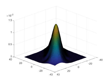
(a) Asymptotic normality: average

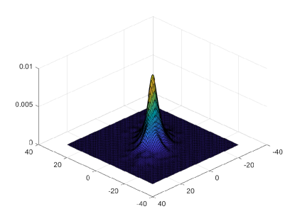
(b) Asymptotic normality: last iterate

Figure 1: Asymptotic normality of SDA

In implementing of Algorithm 1, the step-size $\alpha_{k}=0.5*k^{-0.81}$ and the initial point $x_{0}=(0,0)^{T}$. We first test the asymptotic normality of iterates of SDA in Theorems 2.1 and 2.3. We do 1000 Monte-Carlo simulations of running SDA 1000 iterates and record the estimated density in Figure 1. Figure 1 (a) and Figure 1 (b) depict the estimated densities of the average of iterates SDA and the last iterate of SDA respectively. Figure 1 seems to confirm Theorems 2.1 and 2.3 since we can see that the estimated density is close to the density of a normal distribution and is also confirmed by a Kolmogorov-Smirnov test.

Next, we record the $90\%$ confidence regions with number of iterates $k=1000$, $2000$ and $5000$ respectively. For the stability, we do 50 Monte-Carlo simulations and report the results with the average covariance matrix and the average of iterates. In batch-means method, the sequence $\{a_{m}\}$ is chosen in the form $a_{m}=\left[Cm^{\frac{2}{1-\beta}}\right]_{+}$ with $C=1$. Figure 2 depicts the asymptotic confidence regions of the solution to complementarity problem (4.48), where the red circle ellipse, blue dashed ellipse, green dot ellipse and black solid ellipse denote the confidence regions for number of iterates $1000$, $2000$, $5000$ and the true one respectively. As we can observe from Figure 2 (a), the asymptotic confidence region based on plug-in method at $k=5000$ almost coincides with true confidence region, which indicates the consistency of plug-in method in Theorem 3.1. Compared with Figure 2 (a), the asymptotic confidence region based on batch-means methods is reported in Figure 2 (b), where the asymptotic confidence region at $k=5000$ is small than the true one. The underlying reason may be that the plug-in method employs more information such as gradient of functions and batch-means method uses iterates of SDA only. On the other hand, the batch-means estimator tends to underestimate the variance due to the correlation between batches. Figure 2 (c) verifies the consistency of plug-in method in building the asymptotic confidence regions based on the last iterate of SDA.

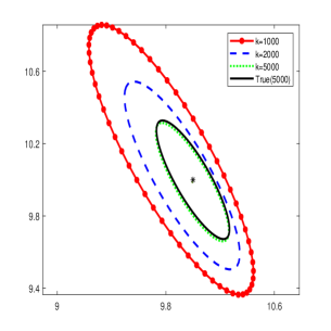
(a) Plug-in

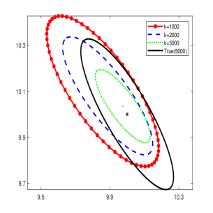
(b) Batch-means

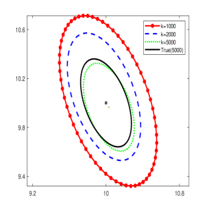
(c) Plug-in (Non-ergodic)

Figure 2: Asymptotic confidence regions for (4.48)

We record the diagonal elements of covariance matrices for number of iterates $1000$, $2000$, $5000$ and the true one respectively in Table 1-2, which characterize the individual confidence intervals of the solution to complementarity problem (4.48). Similar to Figure 2, we can conclude that the plug-in estimators are consistent.

Table 1: Diagonal elements of $\Gamma$

	Plug-in			Batch-means			TRUE
Iterations	1000	2000	5000	1000	2000	5000
$\Gamma(1,1)$	114.07	111.65	112.05	23.25	29.68	27.61	111.78
$\Gamma(2,2)$	86.52	83.99	83.15	22.87	28.61	27.57	83.56

Table 2: Diagonal elements of $\tilde{\Sigma}$

Iterations	1000	2000	5000	TRUE
$\tilde{\Sigma}(1,1)$	30.63	30.36	30.42	30.31
$\tilde{\Sigma}(2,2)$	52.84	51.53	50.94	51.06

We report the coverage probability of $90\%$ confidence regions in Table 3. We estimate the coverage probability by 1000 replications. From Table 3, we can observe that the coverage probabilities of the plug-in methods are getting closer to the nominal level $90\%$ when the number of iterates $k$ grows larger. However, the coverage probabilities of the batch-means method is only $14\%$. The underestimation problem of the batch-means method is because it neglects the correlation between batches. One possible way to handle this problem is to do Monte-Carlo simulation as in Figure 2.

Table 3: The coverage probability of $90\%$ confidence regions

iterations	1000	2000	5000
Plug-in	82	84	88
Batch-means	14	14	20
Plug-in (Non-ergodic)	83	83	86

4.2 Lasso

Least absolute shrinkage and selection operator (Lasso) is a regression analysis method that performs both variable selection and regularization in order to enhance the prediction accuracy and interpretability of the resulting statistical model. We consider lasso on the prostate cancer example [7],

$$\min_{\left(\beta_{0},\beta,t\right)\in{\cal C}}\left(\mathbb{E}\left[Y-\beta_{0}-\sum_{j=1}^{8}\beta_{j}X_{j}\right]^{2}+\lambda\sum_{j=1}^{8}t_{j}\right),$$ (4.49)

where $X\in{\rm I\!R}^{8}$ is the random input vector and $Y\in{\rm I\!R}$ is the response variable. The feasible set ${\cal C}$ of problem (4.49) is given by

$${\cal C}=\left\{\left(\beta_{0},\beta,t\right)\in{\rm I\!R}\times{\rm I\!R}^{8}\times{\rm I\!R}^{8}\mid t_{j}-\beta_{j}\geqslant 0,t_{j}+\beta_{j}\geqslant 0,j=1,\ldots,8\right\}.$$

Similar to [7], we first standardize the predictors to have unit variance and split observations into two parts. One part consists of 67 observations, which are the training set in [37]. We use only these 67 observations in our computation. In implementing of Algorithm 1, we use the same setting of the step-size and initial point in the former example, that is, $\alpha_{k}=0.5k^{-0.81}$ and $x_{0}=0_{17}$. Moreover, the maximum number of iterates is $k=3000$.

Table 4: 95% confidence intervals for $\lambda=0.45$

	Ave-Est	PI CI	BM CI	Last-Est	Non-PI CI
$\beta_{1}$	0.57	[0.55,0.60]	[0.56,0.59]	0.54	[0.44,0.65]
$\beta_{2}$	0.17	[0.13,0.20]	[0.14,0.20]	0.18	[0.09,0.27]
$\beta_{3}$	0	[0,0.04]	[0,0.01]	0	[0,0.10]
$\beta_{4}$	0.01	[0.01,0.01]	[0,0.03]	0	[0,0]
$\beta_{5}$	0.09	[0.09,0.09]	[0.07,0.10]	0.08	[0.08,0.08]
$\beta_{6}$	0	[0,0]	[0,0]	0	[0,0]
$\beta_{7}$	0	[0,0]	[0,0]	0	[0,0]
$\beta_{8}$	0	[0,0]	[0,0]	0	[0,0]

Table 5: 95% confidence intervals for $\lambda=1.49$

	Ave-Est	PI CI	BM CI	Last-Est	Non-PI CI
$\beta_{1}$	0.21	[0.14,0.28]	[0.18,0.24]	0.17	[0.03,0.31]
$\beta_{2}$	0	[0,0]	[0,0]	0	[0,0]
$\beta_{3}$	0	[0,0]	[0,0]	0	[0,0]
$\beta_{4}$	0	[0,0]	[0,0.01]	0	[0,0]
$\beta_{5}$	0	[0,0]	[0,0.02]	0	[0,0]
$\beta_{6}$	0	[0,0]	[0,0.01]	0	[0,0]
$\beta_{7}$	0	[0,0]	[0,0.01]	0	[0,0]
$\beta_{8}$	0	[0,0]	[0,0.01]	0	[0,0]

Tables 4-5 record the $95\%$ individual confidence intervals for lasso parameters with penalty terms $\lambda=0.45$ and $1.49$ respectively. We only report the confidence regions of $\beta_{1},\cdots,\beta_{8}$ as $\beta_{0}$ is the intercept. Similar to [7], we can conclude the importance of predictors in predicting the response and the impact of penalty term $\lambda$ in sparseness of predictors to problem (4.49). Specifically, for $\lambda=0.45$, the individual confidence intervals of $\beta_{1}$ and $\beta_{2}$ do not contain zero and the variances related to $\beta_{4}$ and $\beta_{5}$ are zero. Moreover, the individual confidence intervals of all other variables include zero in them. As $\beta_{4}=0.01$ and $\beta_{5}=0.09$ are close to zero, we may claim that the first two predictors are the most useful ones in predicting the response. On the other hand, for $\lambda=1.49$, only the individual confidence interval of $\beta_{1}$ does not contain zero, which indicates that the first predictor is more important than the second one. We can also observe from Tables 4-5 that lasso shrinks the regression coefficients by imposing a penalty parameter $\lambda$ on their size.

5 Appendix

Lemma 5.1.

[34, Lemma 3.1.1] Suppose $n\times n$-dimension matrix $F_{k}\rightarrow F$, $F$ is a stable matrix, that is, every eigenvalue of $F$ has strictly negative real part. If step-size $\alpha_{k}$ satisfies $\alpha_{k}>0,\alpha_{k}\rightarrow 0$ as $k\rightarrow\infty$, $\sum_{k=1}^{\infty}\alpha_{k}=\infty$ and $n$-dimension vectors $\{e_{k}\},\{\upsilon_{k}\}$ satisfy the following conditions

$$\sum_{k=1}^{\infty}\alpha_{k}e_{k}<\infty,~{}\upsilon_{k}\rightarrow 0,$$

then $\{y_{k}\}$ defined by the following recursion with arbitrary initial value $y_{0}$ tends to zero:

$$y_{k+1}=y_{k}+\alpha_{k}F_{k}y_{k}+\alpha_{k}\left(e_{k}+\upsilon_{k}\right).$$ (5.50)

Lemma 5.2.

[34, Theorem 3.3.1] Let $\{y_{k}\}$ be given by the following recursion with an arbitrarily given initial value:

$$y_{k+1}=y_{k}+\alpha_{k}F_{k}y_{k}+\alpha_{k}\left(e_{k}+\upsilon_{k}\right).$$ (5.51)

Assume the following conditions hold:

• $\alpha_{k}>0,\alpha_{k}\rightarrow 0$ as $k\rightarrow\infty$, $\sum_{k=1}^{\infty}\alpha_{k}=\infty$ and

  $$\alpha_{k+1}^{-1}-\alpha_{k}^{-1}\rightarrow a\geq 0~{}\text{as}~{}k\rightarrow\infty;$$

• $F_{k}\rightarrow F$ and $F+\dfrac{a}{2}\mathbf{I}_{n}$ is stable;

• $${\upsilon_{k}}=o(\sqrt{\alpha_{k}}),\quad e_{k}=\sum_{t=0}^{\infty}C_{t}s_{k-t},s_{t}=0~{}\text{for}~{}t<0,$$

  where $C_{t}$ are $n\times n$ constant matrices with $\sum_{t=0}^{\infty}\|C_{t}\|<\infty$ and $\{s_{k},\mathcal{F}_{k}\}$ is a martingale difference sequence of $n$-dimension satisfying the following conditions

  $$\mathbb{E}\left[s_{k}|\mathcal{F}_{k-1}\right]=0,~{}\sup_{k}\mathbb{E}\left[\|s_{k}\|^{2}\big{|}\mathcal{F}_{k-1}\right]\leq\sigma~{}\text{with}~{}\sigma~{}\text{being a constant,}$$ (5.52)

  $$\lim_{k\rightarrow\infty}\mathbb{E}\left[s_{k}s_{k}^{T}\big{|}\mathcal{F}_{k-1}\right]=\lim_{k\rightarrow\infty}\mathbb{E}\left[s_{k}s_{k}^{T}\right]:=S_{0}$$ (5.53)

  and

  $$\lim_{N\rightarrow\infty}\sup_{k}\mathbb{E}\left[\|s_{k}\|^{2}1_{\{\|s_{k}\|>N\}}\right]=0.$$ (5.54)

  Then $\dfrac{y_{k}}{\sqrt{\alpha_{k}}}$ is asymptotically normal:

  $$\dfrac{y_{k}}{\sqrt{\alpha_{k}}}\xrightarrow{d}\mathcal{N}(0,S),$$

  where

  $$S=\int_{0}^{\infty}e^{(F+(a/2)\mathbf{I}_{n})t}\sum_{k=0}^{\infty}C_{k}S_{0}\sum_{k=0}^{\infty}C_{k}^{T}e^{(F^{T}+(a/2)\mathbf{I}_{n})t}dt.$$

References

• [1] F.Β Facchinei and J.Β Pang, Finite-Dimensional Variational Inequalities and Complementarity Problems. Springer New York, 2003.
• [2] X.Β Chen and M.Β Fukushima, β€œExpected residual minimization method for stochastic linear complementarity problems,” Mathematics of Operations Research, vol.Β 30, pp.Β 1022–1038, 2005.
• [3] G.Β GΓΌrkan, A.Β Y. Demir, and S.Β Robinson, β€œSample-path solution of stochastic variational inequalities,” Mathematical Programming, vol.Β 84, pp.Β 313–333, 1999.
• [4] J.Β Gwinner, β€œA class of random variational inequalities and simple random unilateral boundary value problems - existence, discretization, finite element approximation,” Stochastic Analysis and Applications, vol.Β 18, pp.Β 967–993, 2000.
• [5] X.Β Chen, T.Β K. Pong, and R.Β J. Wets, β€œTwo-stage stochastic variational inequalities: an erm-solutioin procedure,” Mathematical Programming, vol.Β 165, pp.Β 71–112, 2017.
• [6] R.Β T. Rockafellar and R.Β J. Wets, β€œStochastic variational inequalities: Single-stage to multistage,” Mathematical Programming, vol.Β 165, pp.Β 331–360, 2017.
• [7] S.Β Lu, Y.Β Liu, L.Β Yin, and K.Β Zhang, β€œConfidence intervals and regions for the lasso by using stochastic variational inequality techniques in optimization,” Journal of the Royal Statistical Society: Series B (Statistical Methodology), vol.Β 79, pp.Β 589–611, 2017.
• [8] S.Β Lu and A.Β Budhiraja, β€œConfidence regions for stochastic variational inequalities,” Mathematics of Operations Research, vol.Β 38, pp.Β 545–568, 2013.
• [9] M.Β Lamm and S.Β Lu, β€œGeneralized conditioning based approaches to computing confidence intervals for solutions to stochastic variational inequalities,” Mathematical Programming, vol.Β 174, pp.Β 99–127, 2019.
• [10] S.Β Lu, β€œA new method to build confidence regions for solutions of stochastic variational inequalities,” Optimization, vol.Β 63, pp.Β 1431–1443, 2014.
• [11] S.Β Lu, β€œSymmetric confidence regions and confidence intervals for normal map formulations of stochastic variational inequalities,” SIAM Journal on Optimization, vol.Β 24, pp.Β 1458–1484, 2014.
• [12] G.Β Yu, L.Β Yin, S.Β Lu, and Y.Β Liu, β€œConfidence intervals for sparse penalized regression with random designs,” Journal of the American Statistical Association, 2019.
• [13] Y.Β Liu and J.Β Zhang, β€œConfidence regions of stochastic variational inequalities: Error bound approach,” Optimization, 2020. to appear.
• [14] Y.Β Liu, W.Β Yan, and S.Β Zhao, β€œConfidence regions of two‐stage stochastic linear complementarity problems,” International Transactions in Operational Research, vol.Β 29, pp.Β 48–62, 2022.
• [15] H.Β Robbins and S.Β Monro, β€œA stochastic approximation method,” Annals of Mathematical Statistics, vol.Β 22, pp.Β 400–407, 1951.
• [16] K.Β Chung, β€œOn a stochastic approximation method,” Annals of Mathematical Statistics, vol.Β 25, pp.Β 463–483, 1954.
• [17] V.Β Fabian, β€œOn asymptotic normality in stochastic approximation,” Annals of Mathematical Statistics, vol.Β 39, pp.Β 1327–1332, 1968.
• [18] B.Β T. Polyak and A.Β B. Juditsky, β€œAcceleration of stochastic approximation by averaging,” SIAM journal on control and optimization, vol.Β 30, no.Β 4, pp.Β 838–855, 1992.
• [19] M.-h. Hsieh and P.Β Glynn, β€œRecent advances in simulation optimization: confidence regions for stochastic approximation algorithms.,” in Proceedings of the 34th conference on Winter simulation: exploring new frontiers, pp.Β 370–376, 01 2002.
• [20] J.Β Lei and U.Β V. Shanbhag, β€œVariance-reduced accelerated first-order methods: Central limit theorems and confidence statements,” arXiv preprint arXiv:2006.07769, 2020.
• [21] H.Β Jiang and H.Β Xu, β€œStochastic approximation approaches to the stochastic variational inequality problem,” IEEE Transactions on Automatic Control, vol.Β 53, pp.Β 1462 – 1475, 2008.
• [22] A.Β Iusem, A.Β Jofre, R.Β Oliveira, and P.Β Thompson, β€œVariance-based stochastic extragradient methods with linear search for stochastic variational inequalities,” SIAM Journal on Optimization, vol.Β 29, pp.Β 175–206, 2019.
• [23] M.Β Wang and D.Β Bertsekas, β€œIncremental constraint projection methods for variational inequalities,” Mathematical Programming, vol.Β 150, pp.Β 321–363, 2015.
• [24] S.Β Cui and U.Β Shanbhag, β€œOn the analysis of reflected gradient and splitting methods for monotone stochastic variational inequality problems,” in 2016 IEEE 55th Conference on Decision and Control, pp.Β 4510–4515, 2016.
• [25] F.Β Yousefian, A.Β Nedic, and U.Β Shanbhag, β€œOn stochastic mirror-prox algorithms for stochastic cartesian variational inequalities: Randomized block coordinate and optimal averaging schemes,” Set-Valued and Variational Analysis, vol.Β 26, pp.Β 789–819, 2018.
• [26] J.Β Duchi and F.Β Ruan, β€œAsymptotic optimality in stochastic optimization,” The Annals of Statistics, vol.Β 49, pp.Β 21–49, 2021.
• [27] X.Β Chen, J.Β Lee, X.Β Tong, and Y.Β Zhang, β€œStatistical inference for model parameters in stochastic gradient descent,” The Annals of Statistics, vol.Β 48, pp.Β 251–273, 2020.
• [28] M.Β Lamm, S.Β Lu, and A.Β Budhiraja, β€œIndividual confidence intervals for solutions to expected value formulations of stochastic variational inequalities,” Mathematical Programming, vol.Β 165, pp.Β 151–196, 2017.
• [29] Y.Β Nesterov, β€œPrimal-dual subgradient methods for convex problems,” Mathematical Programming, vol.Β 120, pp.Β 221–259, 2009.
• [30] S.Β Lee and S.Β J. Wright, β€œManifold identification in dual averaging for regularized stochastic online learning,” Journal of Machine Learning Research, vol.Β 13, pp.Β 1705–1744, 2012.
• [31] L.Β Xiao, β€œDual averaging methods for regularized stochastic learning and online optimization,” Journal of Machine Learning Research, vol.Β 11, pp.Β 2543–2596, 2010.
• [32] S.Β Zhao, X.Β Chen, and Y.Β Liu, β€œAsymptotic properties of dual averaging algorithm for constrained distributed stochastic optimization,” 2020. manuscript.
• [33] R.Β T. Rockafellar and R.Β Wets, Variational Analysis. Springer, 1998.
• [34] H.Β Chen, Stochastic Approximation and Its Applications. Springer US, 2003.
• [35] G.Β Hewer and C.Β Kenney, β€œThe sensitivity of the stable lyapunov equation,” SIAM Journal on Control and Optimization, vol.Β 26, pp.Β 321–344, 1988.
• [36] W.Β Zhu, X.Β Chen, and W.Β B. Wu, β€œOnline covariance matrix estimation in stochastic gradient descent,” Journal of the American Statistical Association, pp.Β 1–12, 2021.
• [37] T.Β Hastie, R.Β Tibshirani, and J.Β Friedman, The Elements of Statistical Learning: Data Mining, Inference, and Prediction. Springer New York, 2009.