Attribute Surrogates Learning and Spectral Tokens Pooling
in Transformers for Few-shot Learning

Abstract

This paper presents new hierarchically cascaded transformers that can improve data efficiency through attribute surrogates learning and spectral tokens pooling. Vision transformers have recently been thought of as a promising alternative to convolutional neural networks for visual recognition. But when there is no sufficient data, it gets stuck in overfitting and shows inferior performance. To improve data efficiency, we propose hierarchically cascaded transformers that exploit intrinsic image structures through spectral tokens pooling and optimize the learnable parameters through latent attribute surrogates. The intrinsic image structure is utilized to reduce the ambiguity between foreground content and background noise by spectral tokens pooling. And the attribute surrogate learning scheme is designed to benefit from the rich visual information in image-label pairs instead of simple visual concepts assigned by their labels. Our Hierarchically Cascaded Transformers, called HCTransformers, is built upon a self-supervised learning framework DINO and is tested on several popular few-shot learning benchmarks.

In the inductive setting, HCTransformers surpass the DINO baseline by a large margin of 9.7% 5-way 1-shot accuracy and 9.17% 5-way 5-shot accuracy on miniImageNet, which demonstrates HCTransformers are efficient to extract discriminative features. Also, HCTransformers show clear advantages over SOTA few-shot classification methods in both 5-way 1-shot and 5-way 5-shot settings on four popular benchmark datasets, including miniImageNet, tieredImageNet, FC100, and CIFAR-FS. The trained weights and codes are available at https://github.com/StomachCold/HCTransformers.

1 Introduction

Vision transformers have recently become a prominent alternative to convolutional neural networks (CNNs) in many computer vision tasks, including image classification [16, 37, 57], object detection [5, 13, 85, 14, 59], semantic segmentation [69, 58, 83, 15, 23] and etc. However, according to [16, 37], transformers will work in low efficiency on a learning task with only few annotated samples. In this paper, we investigate whether vision transformers can still work well when the amount of labeled training data is extremely limited.

Few-shot learning [62, 19, 39] refers to the problem of learning from a very small amount of labeled data, which is expected to reduce the labeling cost, achieve a low-cost and quick model deployment, and shrink the gap between human intelligence and machine models. The key problem of few-shot learning is how to efficiently learn from the rich information hidden in annotated data. Inspired by the part-whole hierarchical concepts used in GraphFPN [81] and GLOM [25], part layout information of objects/scenes contains various visual information. If it can be embedded in vision transformers to guide the feature learning, we will get discriminative feature representations. Meanwhile, to avoid the concentration of visual information on single concepts, we need to expand the hidden information of image labels into a much more general semantic representation. Then how to mine such latent information and generate a complete description of visual concepts becomes important.

In this paper, we aim to improve the data efficiency in ViT [16] for few-shot image classification. To be specific, we design a meta feature extractor composed of three consecutively cascaded transformers, each of which models the dependency of image regions at different semantic levels. The output tokens of a previous transformer are passed to a spectral tokens pooling layer to produce the input tokens for the subsequent. The spectral tokens pooling is partly based on spectral clustering [44, 74], where features of tokens within same clusters are averaged to generate new token descriptors for the subsequent transformer. The motivation behind the spectral tokens pooling is to bring the image segmentation hierarchy into transformers. That means when the transformer performs self-attention, it needs to consider the image layout not simply through the positional embedding, but from the semantic relationship of different image regions. In our implementation, each token can be thought to represent some specific region within an image. We treat every token as a vertex in a graph and the token similarity matrix describes the edge connectivity. Thus, the spectral tokens pooling becomes an image segmentation problem and can be solved efficiently as that in normalized cut [55].

In practice, we insert two spectral tokens pooling layers between three transformers. Since they capture the semantic dependencies of tokens in different hierarchies, we call them Hierarchically Cascaded Transformers (written as HCTransformers). Besides, we don’t utilize the supervision information directly as that in other state-of-the-art few-shot learning methods [42, 53, 84, 67]. Instead, we introduce a latent attribute surrogates learning scheme to learn robust representations of visual concepts. We hallucinate some latent semantic surrogates for each class to guide the learning of deep models. The latent semantic surrogates also have learnable parameters that can be jointly learnt with the parameters of transformers end-to-end. In fact, it’s a kind of weakly supervised learning by generalizing image-level annotation into attribute-level supervision. Based on such a latent attribute surrogate learning scheme, we avoid directly mapping an image into a single visual concept from a predefined set of object categories.

The contributions of this paper are as follows:

• We employ ViT as the meta feature extractor for few-shot learning and propose Hierarchically Cascaded Transformers (HCTransformers), which greatly improve the data efficiency through attribute surrogates learning and spectral tokens pooling.

• We propose a latent supervision propagation scheme for transformers in a weakly supervised manner. It converts the image label prediction task into a latent attribute surrogates learning problem. In this way, both the class and patch tokens can be supervised efficiently.

• We introduce a novel spectral tokens pooling scheme to transformers. It models the dependency relationship of image regions in both the spatial layout and the semantic relationship. Due to such a mechanism, ViT can learn much more discriminative features at different semantic hierarchies.

• Experiments demonstrate that our HCTransformers surpass its DINO baseline on miniImageNet [62], and outperform other state-of-the-art algorithms significantly on multiple few-shot learning benchmarks, including miniImageNet [62], tieredImageNet [52], and CIFAR-FS [4] and FC-100 [45].

2 Related Work

Meta-/Few-shot Learning. Meta-learning or “learning to learn” [47, 2] refers to improving a learning task by learning over multiple learning episodes. Meta-learning has become the dominant paradigm for few-shot learning [18, 60]. Various meta-learning based methods have been proposed for few-shot image classification, such as MAML [18], REGRAB [49], TAML [27], MetaOptNet [33], and etc. However, according to [10, 20, 48], training CNNs from scratch with meta-learning shows inferior performance in comparison to fine-tuning a CNN feature extractor pre-trained in a standard manner. There are also other methods focusing on better feature extraction [68], additional knowledge [65], knowledge transfer [34], and graph neural networks [31]. Different from previous meta-learning methods, we introduce the inherent semantic hierarchies of images into transformers, and supervise the parameter learning with latent attribute surrogates. By this way, we alleviate the overfitting problem and get impressive results.

Tokens Pooling in Transformers. ViT [16] directly applies transformer architecture into vision tasks by splitting input image into $16\times 16$ tokens via patch embedding. Despite impressive results on several vision benchmarks, vanilla transformer architectures focus on attending global information while neglecting local connections, which hinders the use of fine-grained image features thus leading to their data-hungry nature. Many subsequent works address this issue by establishing a progressive shrinking pyramid that allows models to explicitly process low-level patterns. There is a group of approaches that merge tokens within each fixed window into one to reduce the number of tokens [37, 63, 66, 24, 76, 46, 8]. In contrast, the second group of methods drops this constraint and introduces more flexible selection scheme [50, 9, 77, 43]. While our HCTransformers allow tokens to be adaptively merged with their neighboring tokens according to their spatial layout and semantic similarities.

Supervise Patch Tokens in Transformers. ViT[16] adds a $[cls]$ token to globally summarize the integral information of patch tokens and only this token directly receives supervision signals. However, other tokens maintain the ability to express distinctive patterns and may delicately assist final prediction. Some works proposed to remove the $[cls]$ token and construct a global token by integrating patch tokens via certain average pooling operation [37, 46, 51, 8]. LV-ViT [29] explored the possibility to jointly utilize $[cls]$ token and patch tokens. It reformulates the classification task with the token labeling problem. Likewise, So-ViT [70] applied a second-order and cross-covariance pooling to visual tokens, which is combined with the $[cls]$ token for final classification. Our method shares similar intuition with these two methods, but the difference is apparent. We integrate patch tokens as a weighted sum where scores are calculated based on their connections with the global $[cls]$ token, which aims to mostly utilize significant patch tokens. Besides, we suppose the integrated patch tokens do not share the feature space with the $[cls]$ token and supervise them within their own feature space.

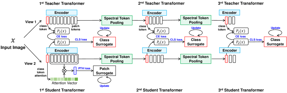
Figure 1: Illustration of the overall structure. HCTransformers contain three sets of cascaded transformer networks, each corresponding to a teacher-student knowledge distillation framework. During training, every student transformer builds and updates a surrogate descriptor for each category. The patch tokens integrated through the attention map are also used to generate patch surrogate descriptors in the first stage. In between every two transformer sets, a spectral tokens pooling layer is used to down-sample the patch token number by $\frac{1}{2}$ for information aggregation.

3 Hierarchically Cascaded Transformers

3.1 Overview

The core of HCTransformers is to make the full usage of the annotated data to train transformers as a strong meta feature extractor for few-shot learning. To benefit from existing self-supervised learning techniques [22, 7], we use DINO [7] as our base learning framework and multi-crop strategy [6] to conduct knowledge distillation [26]. In the pretraining stage of few-shot learning, we can access image labels. We design a latent attribute surrogates learning scheme for both patch tokens and the $[cls]$ tokens to avoid directly learning from labels. To incorporate the semantic hierarchy into transformers, we insert a spectral tokens pooling layer between two ViTs [16]. The output similarity matrix of patches can be used to conduct spectral clustering to segment patches into disjoint regions. Then the feature average of patches in the same region is treated as a new token feature, which captures higher-level semantic information. In Fig. 1, we illustrate the complete pipeline of our proposed method.

3.2 Preliminary

Similar to BYOL [22], DINO [7] employs a knowledge distillation framework for self-supervised learning with two homogeneous networks: teacher and student, where the teacher’s parameter ($\theta_{t}$) is an exponential moving average results of the updated student’s parameter ($\theta_{s}$) on the foundation of ViT [16] architecture. Each network consists of a transformer encoder and a classification head (i.e., a multi-layer perceptron and one fully connected layer).

Given an input image $x\in\mathbb{R}^{H\times W\times C}$, DINO first reshapes $x$ into a sequence of flattened 2D patch tokens $t_{p}\in\mathbb{R}^{N\times D}$. $t_{p}$ is then concatenated with a learnable class token $t_{c}\in\mathbb{R}^{1\times D}$ for an augmented sequence $T\in\mathbb{R}^{(N+1)\times D}$. Here, $\{H,W\}$ denote the spatial resolution of the input image, $C$ stands for the image channel number. $N=HW/P^{2}$ is the resulting number of patches, where $P$ denotes the patch size. $D$ represents the encoded feature dimension. After passing through the transformer encoder, the sequence enhances its representation through self-attention. We denote the enhanced patch tokens as $f_{p}(x)\in\mathbb{R}^{N\times D}$. Likewise, the enhanced $[cls]$ token is denoted as $f_{c}(x)\in\mathbb{R}^{1\times D}$. Moreover, the token similarity matrix ${\bf A}\in\mathbb{R}^{(N+1)\times(N+1)}$ can be acquired from the self-attention process. Afterwards, only the encoded $[cls]$ token is used for final prediction. We pass this $[cls]$ token to the projection head to map it into a higher $D^{\prime}$-dimension, which is denoted as $P(x)$.

Besides, DINO employs a multi-crop training augmentation scheme. For any given image $x$, it constructs a set $V$ of the subregions, including two global views, $x_{1}^{g}$ and $x_{2}^{g}$ and $m$ local views. DINO minimizes the following loss to encourage the “local-to-global” prediction consistency:

$$\mathcal{L}_{\rm DINO}=\frac{1}{M}\sum\limits_{x_{g}\in\left\{x_{1}^{g},x_{2}^{g}\right\}}\sum\limits_{x^{\prime}\in V,\ x^{\prime}\neq x_{g}}-P_{t}(x_{g})\ {\rm\log}{P_{s}(x^{\prime})},$$ (1)

where $M$ is the pair number $2\times(m+1)$. $P_{t}(x_{g})$, $P_{s}(x^{\prime})$ are the outputs of teacher and student networks, respectively.

3.3 Jointly Attribute Surrogates and Parameters Learning

We design a latent supervision propagation scheme for transformers to avoid supervising the parameter learning only through a quite limited amount of one-hot labels. For each visual concept $y$ in the label space, we aim to learn a semantic attribute surrogate $z(y)\in\mathbb{R}^{1\times D^{\prime}}$ for it,

$$y\rightarrow z(y),$$ (2)

where $D^{\prime}$ is the surrogate descriptor dimension. When there are $C$ classes, the surrogate descriptors ${\bf Z}\in\mathbb{R}^{C\times D^{\prime}}$ would contain $C$ entries. During the learning process, the supervision is passed through surrogates to supervise the student’s parameter learning. At the same time, these surrogates need to be learnt at the same time. Supposing the supervised learning objective of the student is $\mathcal{L}_{\rm surr}$, then the parameters $\theta_{s}$ of the student and its associated surrogates can be updated with the following equations

$$\theta_{s}^{t+1}=\theta_{s}^{t}-\gamma_{1}\frac{\partial\mathcal{L}_{\rm surr}}{\partial\theta_{s}^{t}},$$ (3)

$$z(y)^{t+1}=z(y)^{t}-\gamma_{2}\frac{\partial\mathcal{L}_{\rm surr}}{\partial z(y)^{t}},$$ (4)

where $\gamma_{1}$ and $\gamma_{2}$ are the learning rates. During the initialization, both $\theta_{s}$ and $\bf Z$ are initialized with Gaussian noises. Following the settings in DINO  [7], we use the AdamW optimizer [38] with momentum to update both $\theta_{s}$ and ${\bf Z}$ with linear scaling rule [21], which is a slightly different with that in the center loss [64].

To make the fully advantage of transformers, we learn semantic attribute surrogates for both patch and class tokens respectively.

Supervise the Class Token. In DINO [7] and other knowledge distillation methods, the student network produces probability over $D^{\prime}$ dimensions. Different from traditional supervised learning paradigms, $D^{\prime}$ is set to a quite large number without considering the dataset’s real class number. In this paper, we set $D^{\prime}=8192$. To be consistent with the teacher-student knowledge distillation in DINO, we use the surrogate loss to supervise the probability distribution learning for every class. Then the surrogate descriptor ${z_{c}}(y)\in\mathbb{R}^{8192}$ of the class $y$ is a vector on 8192 dimensions. We normalize ${z_{c}}(y)$ with the Softmax operation to get an attribute distribution $\overline{{z_{c}}}(y)$. Following the annotations in Eq. 1, the class token loss becomes:

$$\mathcal{L}^{\rm cls}_{\rm surr}=\frac{1}{2}\sum\limits_{x_{g}\in\left\{x_{1}^{g},x_{2}^{g}\right\}}D_{\rm KL}(P_{s}(x_{g})||\overline{{z_{c}}}(y)),$$ (5)

where $y$ is the label of the input image $x$, and $D_{\rm KL}$ is the Kullback–Leibler divergence. Note that only global views are involved here considering that local views may introduce negative effects when updating class centers due to the loss of information.

Supervise Patch Tokens. In transformers, patch tokens are hard to be supervised due to the lack of patch-level annotations. To supervise patch tokens, we firstly aggregate the patch token features $f_{p}(x)$ to generate a global descriptor of an image $x$ by applying the attention map ${\bf A}_{c}(x)\in\mathbb{R}^{1\times N}$:

$$F_{p}(x)={\bf A}_{c}(x)f_{p}(x)$$ (6)

where ${\bf A}_{c}(x)$ denotes the similarity matrix that can be acquired by calculating the similarity between the $[cls]$ token and each patch token. ${F}_{p}(x)\in\mathbb{R}^{1\times D}$ is the patch token feature. We treat each entry in ${F}_{p}(x)$ as a description about some semantic attributes, and normalize it with a Softmax operation to convert it into an attribute distribution ${\overline{F}}_{p}(x)={\rm Softmax}~{}{F}_{p}(x)$. Similarly with that in the class token, we have an attribute surrogate $z_{p}\left(y\right)$ for each class. The patch token loss becomes:

$$\mathcal{L}_{\rm surr}^{\rm pth}=\frac{1}{2}\sum\limits_{x_{g}\in\left\{x_{1}^{g},x_{2}^{g}\right\}}D_{\rm KL}({\overline{F}}_{p}(x)||\overline{z}_{p}\left(y\right)),$$ (7)

where $\overline{z}_{p}\left(y\right)={\rm Softmax}~{}{z}_{p}\left(y\right)$. Only the global views are applied for same consideration as aforementioned.

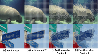
Figure 2: Visualized tokens pooling results. After spectral tokens pooling operations, adjacent tokens with similar semantics are clustered into one. (c) and (d) shows that our clustering results are well consistent with the image’s basic structure. The pixel colors in the same cluster are averaged.

3.4 Spectral Tokens Pooling

Multi-scale hierarchical structures have been proven effective in both convolutional neural networks [36, 28] and transformers [37]. We aim to improve the feature discriminative ability through embedding hierarchical structures into transformers. Different from the grid pooling scheme in Swin Transformer [37], here we exploit the irregular pooling method to match the image structures with more flexibility. Since transformers will generate self-attention matrices among tokens, it provides a strong prior for spectral clustering algorithms to segment tokens according to both their semantic similarities and the spatial layout. So we propose a spectral clustering-based pooling method, called spectral tokens pooling.

For the $N$ patch tokens in a ViT, we retrieve attention matrix between patches ${\bf A_{p}}$ $\in\mathbb{R}^{N\times N}$ from $\bf A$. To bring in spatial consistency, we maintain an adjacency matrix ${\bf H}\in\mathbb{R}^{N\times N}$ to reflect the neighborhood relationship. In our design, only 8-connected neighboring tokens are connected with the center token. We use the following formula to retrieve a symmetric $\bf S$ matrix.

$$\bf S=\bf A_{p}\odot\bf H+\bf A_{p}^{\mathsf{T}}\odot\bf H^{\mathsf{T}}.$$ (8)

Through the spatial constraint, the $\bf S$ matrix can be viewed as a sparse matrix for computation acceleration. We then perform the Softmax operation on each row of $\bf S$ to get the final adjacency weight matrix $\bf S^{\prime}$. The spectral clustering algorithms [44, 55, 72] are exploited to partition patch tokens into $N^{\prime}$ clusters $\mathcal{T^{prime}}=\left\{\mathcal{T}_{1},\mathcal{T}_{2},...,\mathcal{T}_{N^{\prime}}\right\}$ and generate new tokens with Algorithm 1. During the backward stage, gradients of token clusters are copied to each of the averaged tokens. We implement the spectral tokens pooling with PyTorch. Fig. 2 visualizes results of two consecutive spectral tokens pooling.

Input: Tokens $\bf T\in\mathbb{R}^{N\times D}$, adjacency weight matrix $\bf S^{\prime}\in\mathbb{R}^{N\times N}$, number $N^{\prime}$ clusters to construct.

Output: Tokens $\bf T^{\prime}\in\mathbb{R}^{N^{\prime}\times D}$.

1 Compute the normalized Laplacian $\bf L$ from $\bf S^{\prime}$;

2 Compute the first $N^{\prime}$ eigenvectors $\mu_{1},\mu_{2},...,\mu_{N^{\prime}}$ of L;

3 Construct a matrix $\bf U\in\mathbb{R}^{N\times N^{\prime}}$ to contain the vectors $\mu_{1},\mu_{2},...,\mu_{N^{\prime}}$ as columns;

4 For $i=1,...,n$, let $v_{i}\in\mathbb{R}^{N^{\prime}}$ be the vector corresponding to the $i$-th row of $U$;

5 Cluster the points $(v_{i})_{i=1,...,N}\in\mathbb{R}^{N^{\prime}}$ with K-means algorithm into clusters $\mathcal{T}=\left\{\mathcal{T}_{1},\mathcal{T}_{2},...,\mathcal{T}_{N^{\prime}}\right\}$;

6 Features of tokens in the same clusters are averaged to generate new tokens $\bf T^{\prime}\in\mathbb{R}^{N^{\prime}\times D}$.

Algorithm 1 Spectral Tokens Pooling Algorithm

3.5 Training Strategy of HCTransformers

In our design, two spectral tokens pooling layers are inserted into three different transformers. That means the outputs of previous transformers are sent to the subsequent transformers after performing pooling operations. In this way, tokens are organized with different semantic hierarchies. For different transformers, we set the output token numbers to 784, 392, 196, respectively.

Since computing eigenvectors in spectral tokens pooling is time consuming ( 21.3 im/sec and 75.2 im/sec in two pooling layers respectively), we don’t jointly all the three transformers end-to-end. The training is divided into two stages. In the first stage, we train the first two transformer as the same setting as DINO [7] with the loss function bellow,

$$\mathcal{L}_{\rm stage1}=\mathcal{L}_{\rm DINO}+\alpha\mathcal{L}^{\rm cls}_{\rm surr}+\beta\mathcal{L}^{\rm pth}_{\rm surr}.$$ (9)

Then we frozen parameters of the first two transformer and train the subsequent two sets of transformers jointly with the same loss function in Eq. 10. We only supervise on the $[cls]$ token for higher efficiency in the second stage. Since features produced by the first transformer already have strong discriminative ability, the training of subsequent transformers converges quickly in several epochs.

$$\mathcal{L}_{\rm stage2}=\mathcal{L}_{\rm DINO}+\alpha\mathcal{L}^{\rm cls}_{\rm surr}$$ (10)

The weights $\alpha$ and $\beta$ are set to 1 and 0.1 in this work.

Method	backbone	miniImagenet		tieredImagenet
		1-shot	5-shot	1-shot	5-shot
DeepEMD[78]	ResNet-12	65.91 $\pm$ 0.82	82.41 $\pm$ 0.56	71.16 $\pm$ 0.87	86.03 $\pm$ 0.58
IE[53]	ResNet-12	67.28 $\pm$ 0.80	84.78 $\pm$ 0.52	72.21 $\pm$ 0.90	87.08 $\pm$ 0.58
DMF[71]	ResNet-12	67.76 $\pm$ 0.46	82.71 $\pm$ 0.31	71.89 $\pm$ 0.52	85.96 $\pm$ 0.35
BML[84]	ResNet-12	67.04 $\pm$ 0.63	83.63 $\pm$ 0.29	68.99 $\pm$ 0.50	85.49 $\pm$ 0.34
PAL[41]	ResNet-12	69.37 $\pm$ 0.64	84.40 $\pm$ 0.44	72.25 $\pm$ 0.72	86.95 $\pm$ 0.47
METAQDA[80]	WRN	67.38 $\pm$ 0.55	84.27 $\pm$ 0.75	74.29 $\pm$ 0.66	89.41 $\pm$ 0.77
TPMN[67]	ResNet-12	67.64 $\pm$ 0.63	83.44 $\pm$ 0.43	72.24 $\pm$ 0.70	86.55 $\pm$ 0.63
MN + MC[79]	ResNet-12	67.14 $\pm$ 0.80	83.82 $\pm$ 0.51	74.58 $\pm$ 0.88	86.73 $\pm$ 0.61
DC[75]	WRN-28-10	68.57 $\pm$ 0.55	82.88 $\pm$ 0.42	78.19 $\pm$ 0.25	89.90 $\pm$ 0.41
MELR[17]	ResNet-12	67.40 $\pm$ 0.43	83.40 $\pm$ 0.28	72.14 $\pm$ 0.51	87.01 $\pm$ 0.35
COSOC[40]	ResNet-12	69.28 $\pm$ 0.49	85.16 $\pm$ 0.42	73.57 $\pm$ 0.43	87.57 $\pm$ 0.10
CSEI[35]	ResNet-12	68.94 $\pm$ 0.28	85.07 $\pm$ 0.50	73.76 $\pm$ 0.32	87.83 $\pm$ 0.59
CNL[82]	ResNet-12	67.96 $\pm$ 0.98	83.36 $\pm$ 0.51	73.42 $\pm$ 0.95	87.72 $\pm$ 0.75
Baseline-Cosine	ViT-S	52.92 $\pm$ 0.17	65.04 $\pm$ 0.14	66.04 $\pm$ 0.20	78.05 $\pm$ 0.16
Ours-Cosine	ViT-S	74.74 $\pm$ 0.17	85.66 $\pm$ 0.10	79.67 $\pm$ 0.20	89.27 $\pm$ 0.13
Ours-Classifier	ViT-S	74.62 $\pm$ 0.20	89.19 $\pm$ 0.13	79.57 $\pm$ 0.20	91.72 $\pm$ 0.11

Table 1: Comparison with the state-of-the-art 5-way 1-shot and 5-way 5-shot performance with 95% confidence intervals on miniImagenet and tieredImagenet. ViT-S is our baseline. Top three results are shown in red, blue and green based on their relative rankings.

4 Experiments

4.1 Datasets

We perform experiments on four popular benckmark datasets for few-shot classification, including miniImageNet [62], tieredImageNet [52], CIFAR-FS [4], and FC100 [45]. miniImageNet [62] contains 100 classes from the ImageNet [54] [4], randomly split into 64 bases, 16 validation, and 20 novel classes, and each class contains 600 images. tieredImageNet [52] contains 608 classes from 34 super-classes of the ImageNet, randomly split into 351 bases, 97 validation, and 160 novel classes. There are 779,165 images in total. CIFAR-FS [4] contains 100 classes from the CIFAR100 [32], randomly split into 64 bases, 16 validation, adn 20 novel calsses, and each class contains 600 images. FC100 [45] contains 100 classes from 36 super-classes of the CIFAR100, where 36 super-classes were split into 12 base (including 60 classes), 4 validation (including 20 classes) and 4 novel (including 20 classes) super-classes, and each class contains 600 images.

4.2 Implementation Details

All experiments are run on ViT-S/8 (8 is the size of each patch). We adopt the multi-crop strategy of DINO, we randomly crop and resize an image to 2 global images at resolution $224^{2}$ and 8 local images at resolution $96^{2}$. The teacher networks take in the 2 global views and the student networks take in all 10 image corps. In the first stage, to train a reliable meta feature extractor, we set $\alpha$ and $\beta$ to 1 and 0.1, respectively, then the gradients produced by $\mathcal{L}_{\rm DINO}$, $\mathcal{L}^{\rm cls}_{\rm surr}$ and $\mathcal{L}^{\rm pth}_{\rm surr}$ are in the same order of magnitude. Other specific parameters are inherited from DINO. In the second stage for spectral tokens pooling, we employ K-mean++ to conduct clustering. The $[cls]$ token input for the latter pooling transformer is initialized by the former’s transformed $[cls]$ token for efficient training.

Evaluation. We evaluate experiments on 5-way 1-shot and 5-way 5-shot classification. For each task, we randomly select 5 categories. In each category, we use 1 or 5 labeled images as support data and another 599 or 595 unlabeled images of the same category as novel data. The reported results are the averaged classification accuracy over 10,000 tasks. During the meta test, we don’t fuse the features of three student transformers. We actually use the validation set to select the class token features of the second student transformer to generate the final feature representation. For module ablations, we use the class token feature of individual transformer as the output. We use the simple Cosine classifier and the linear classifier in S2M2[42] to predict query labels.

4.3 Comparisons with State-of-the-art Results

Tab. 3 shows the 1-shot and 5-shot comparison results with the latest state-of-the-art (SOTA) methods on miniImagenet [62] and tieredImagenet [52]. We outperform previous SOTA results by great margins with simple classifiers. For instance, on miniImagnet, HCTransformers surpasses SOTAs by 5.37% (1-shot) and 4.03% (5-shot), respectively. When we turn to tieredImagenet, our method outperforms the most recent DC [75] by 1.48% and 1.81% on 1-shot and 5-shot, respectively. Compared with DC which borrows class statistics from the base training set, we don’t need to do this and our classifier is lightweight. Another evidence is that the margin between our method and the third-best approach is 5.09% on 1-shot, which helps validate our contribution. We give credit to our network structure for such impressive results, which can learn a lot of inherent information in data and maintain good generalization ability.

Tab. 2 and Tab. 3 display the results on small-resolution datasets, i.e., CIFAR-FS and FC100. HCTransformers show comparable or better results in these low-resolution settings: 1-shot ($1.02\%$) and 5-shot ($0.76\%$) on CIFAR-FS; 1-shot (0.51%) and 5-shot (1.12%) on FC100. We observe that on the small resolution datasets, we don’t surpass previous SOTA methods too much. We attribute this to the patching mechanism of ViT. When the image resolution is small, such as $32^{2}$, it is difficult to retrieve useful representation from cropped patches with limited numbers of real pixels. Similarly, DeepEMD [78] also mentioned that patch cropping would have negative impacts on the small resolution images. However, our method still achieves the new SOTA results on both of these two benchmarks.

Method	backbone	CIFAR-FS
		1-shot	5-shot
DSN-MR[56]	ResNet-12	75.60 $\pm$ 0.90	86.20 $\pm$ 0.60
TPMN[67]	ResNet-12	75.50 $\pm$ 0.90	87.20 $\pm$ 0.60
IE[53]	ResNet-12	77.87 $\pm$ 0.85	89.74 $\pm$ 0.57
PSST[12]	WRN-28-10	77.02 $\pm$ 0.38	88.45 $\pm$ 0.35
BML[84]	ResNet-12	73.45 $\pm$ 0.47	88.04 $\pm$ 0.33
PAL[41]	ResNet-12	77.10 $\pm$ 0.70	88.00 $\pm$ 0.50
MN + MC[79]	ResNet-12	74.63 $\pm$ 0.91	86.45 $\pm$ 0.59
RENet[30]	ResNet-12	74.51 $\pm$ 0.46	86.60 $\pm$ 0.32
METAQDA[80]	WRN	75.95 $\pm$ 0.59	88.72 $\pm$ 0.79
ConstellationNet[73]	ResNet-12	75.40 $\pm$ 0.20	86.80 $\pm$ 0.20
Baseline-Cosine	ViT-S	57.75 $\pm$ 0.16	72.15 $\pm$ 0.12
Ours-Cosine	ViT-S	78.89 $\pm$ 0.18	87.73 $\pm$ 0.11
Ours-Classifier	ViT-S	78.88 $\pm$ 0.18	90.50 $\pm$ 0.09

Table 2: Comparison with the state-of-the-art 5-way 1-shot and 5-way 5-shot performance with 95$\%$ confidence intervals on CIFAR-FS. Top three results are shown in red, blue and green

.

Method	backbone	FC100
		1-shot	5-shot
DeepEMD[78]	ResNet-12	46.47 $\pm$ 0.78	63.22 $\pm$ 0.71
IE[53]	ResNet-12	47.76 $\pm$ 0.77	65.30 $\pm$ 0.76
BML[84]	ResNet-12	45.00 $\pm$ 0.41	63.03 $\pm$ 0.41
ALFA+MeTAL[3]	ResNet-12	44.54 $\pm$ 0.50	58.44 $\pm$ 0.42
MixtFSL[1]	ResNet-12	41.50 $\pm$ 0.67	58.39 $\pm$ 0.62
PAL[41]	ResNet-12	47.20 $\pm$ 0.60	64.00 $\pm$ 0.60
TPMN[67]	ResNet-12	46.93 $\pm$ 0.71	63.26 $\pm$ 0.74
MN + MC[79]	ResNet-12	46.40 $\pm$ 0.81	61.33 $\pm$ 0.71
ConstellationNet[73]	ResNet-12	43.80 $\pm$ 0.20	59.70 $\pm$ 0.20
Baseline-Cosine	ViT-S	40.83 $\pm$ 0.15	50.93 $\pm$ 0.15
Ours-Cosine	ViT-S	48.27 $\pm$ 0.15	61.49 $\pm$ 0.15
Ours-Classifier	ViT-S	48.15 $\pm$ 0.16	66.42 $\pm$ 0.16

Table 3: Comparison with the state-of-the-art 5-way 1-shot and 5-way 5-shot performance with 95$\%$ confidence intervals on FC100. Top three results are shown in red, blue and green.

Learnable Parameters Comparision. In Table 4, we can find that more learnable parameters don’t lead to better performance directly. The backbone of METAQDA${}_{\;\rm{\,ICCV21}}$ has much more parameters than IE${}_{\;\rm{\,CVPR21}}$ and HCTransformers, but get inferior performances. Compared with the ViT-S backbone and DINO${}_{\;\rm{\,ICCV21}}$, HCTransformers get impressive improvements. It indicates that the proposed attribute surrogates learning and spectral tokens pooling are very important to utlize the strong learning abilities of transformers. Although we have more parameters than IE${}_{\;\rm{\,CVPR21}}$ with the ResNet-12 backbone, we argue that our contribution is improving the data efficiency for transformers, and thus make them suitable for few-shot learning.

Method	Backbone	Params	1-shot	5-shot
IE${}_{\;\rm{\,CVPR21}}$	ResNet-12	12.4M	69.28±0.80	85.16±0.52
METAQDA${}_{\;\rm{\,ICCV21}}$	WRN-28-10	36.5M	67.38±0.55	84.27±0.75
Cosine Distance	ResNet-50	23M	59.28±0.20	72.68±0.16
Cosine Distance	ViT-S	21M	52.92±0.17	65.04±0.14
DINO${}_{\;\rm{\,ICCV21}}$(baseline)	ViT-S	21M	61.57±0.16	75.51±0.12
HCTransformers 1	ViT-S	21M	71.27±0.17	85.66±0.10
HCTransformers 2	ViT-S	21M	74.74±0.17	89.19±0.13
HCTransformers 3	ViT-S	21M	72.66±0.17	85.66±0.10

Table 4: Comparison of state-of-the-art algorithms with different backbones on miniImagenet.

Computational Cost of Spectral Tokens Pooling. In Table 5, we list the training time cost of different modules in HCTransformers. It can be find that the spectral tokens pooling are relatively slow in our whole pipeline. But when compared with the first training stage, the time spent is still affordable because it needs only several epochs to train the second and third sets of transformers.

	Stage 1(400 epoch)	Stage 2(2 epoch)		Stage 3(2 epoch)
	ViT	Pooling	ViT	Pooling	ViT
Time	21.1h	0.33 h	0.25 h	0.12 h	0.09 h

Table 5: The amount of training time spent at each stage on 8 Nvidia RTX 3090 GPUs on miniImageNet.

4.4 Ablation Studies

To investigate the contributions of different components, we conduct thorough experiments in this section. In the following, we use the cosine classifier for query labels prediction.

Method	Loss	1-shot	5-shot
DINO	-	$61.57\pm 0.16$	75.51 $\pm$ 0.12
DINO	CE	66.81 $\pm$ 0.17	80.27 $\pm$ 0.12
DINO	PTH	63.17 $\pm$ 0.16	78.59 $\pm$ 0.12
DINO	CLS	68.95 $\pm$ 0.17	82.83 $\pm$ 0.11
Ours	CLS+PTH	71.27 $\pm$ 0.17	84.68 $\pm$ 0.10

• CE: cross-entropy loss, PTH: pth loss, CLS: cls loss.

Table 6: The results of the first student transformer trained with different supervision on miniImagenet. All models are based on the DINO baseline. ”CE” stands for the combination of a cross-entropy loss (as that in ViT [16]) and the DINO loss. ”PTH” stands for the combination of the patch surrogate loss and the DINO loss. ”CLS” stands for the combination of the class surrogate loss and the DINO loss. ”CLS+PTH” stands for the full combination of the class surrogate loss, the patch surrogate loss and the DINO loss.

$\beta$	1-shot	5-shot
1	61.45 $\pm$ 0.16	78.59 $\pm$ 0.12
0.1	71.27 $\pm$ 0.17	84.68 $\pm$ 0.10
0.01	70.40 $\pm$ 0.16	84.07 $\pm$ 0.10

Table 7: Test of the choice of different $\beta$ about the patch surrogate loss in the first student transformer on miniImagenet.

Figure 3: Visualizing features of DINO and HTransformers by t-SNE [61] on both train and validation sets on miniImagenet. Points with the same color correspond to the same category. (a) and (b) show that when equipped with semantic surrogates, more distinctive features can be learned compared with DINO baseline. Feature distribution patterns on validation set(i.e., (c) and (d)) illustrate that our method can generalize well on unseen data.

Whether the latent supervision propagation is helpful? To demonstrate the effectiveness of our proposed latent supervision propagation scheme, we conduct a series of experiments with different settings on miniImagenet in the first training stage. Results in Tab. 6 show that our proposed scheme greatly improves over DINO baseline by 9.70% for 1-shot setting and 9.17% for 5-shot setting. To explore if the patch and class surrogate losses bring in benefits, we replace them with the commonly used cross entropy loss as in ViT to supervise the parameter learning together with the DINO loss. The 5-way 1-shot and 5-way 5-shot performances drop by 4.46% and 4.41% respectively. It validates our assumption that when there is few labeled data, supervising transformers with one-hot vectors will show inferior generalization ability.

We also test the effects of the class and patch surrogate losses individually. When we remove the patch token loss for Eq. 9, the 5-way 1-shot and 5-way 5-shot accuracy drop by 2.3% and 1.85%. If we remove the class token loss from Eq. 9, the performances drop to 63.17% and 78.59% which indicates that the class surrogate loss is key to get good performance. All these experiments show that the two surrogate losses are effective in training transformers.

We try different weights $\beta$ for the patch surrogate loss by setting it to 1, 0.1, 0.01, respectively. Tab. 7 shows that setting $\beta$ to 0.1 is most suitable for the current setting.

resolution/patch	1-shot	5-shot
$56^{2}/2$	71.99 $\pm$ 0.17	85.04 $\pm$ 0.11
$112^{2}/4$	72.80 $\pm$ 0.17	85.93 $\pm$ 0.11
$224^{2}/8$	73.28 $\pm$ 0.16	86.49 $\pm$ 0.11

Table 8: The performances of the first student transformer which takes in images with different resolutions/patch sizes on CIFAR-FS.

model	$84^{2}$	$224^{2}$
IE [53]	66.82 $\pm$ 0.80	60.88 $\pm$ 0.81
DeepEMD [78]	65.91 $\pm$ 0.82	63.07 $\pm$ 0.81

Table 9: The influence of image resolutions on two state-of-the-art methods on miniImagenet for 5-way 1-shot classification.

How is the input resolution affects the results? In our implementation, images are resized into $224\times 224$, which is higher than traditional CNN-based methods, such as IE [53, 42]. Multiple experiments are conducted to prove such a resolution yields is suitable for ViT [16], while other state-of-the-art methods including IE [53] and DeepEMD [78], fail to utilize high-resolution inputs. To test the performance of our HCTransformers when taking in images with different resolutions, we conduct experiments on CIFAR-FS [4]. We resize images into $32\times 32$ to $54\times 54$, $112\times 112$, and $224\times 224$. The patch sizes are then $2\times 2$,$4\times 4$ and $8\times 8$ respectively. Results of different settings are listed in Tab. 8, showing that higher resolutions lead to better performance. We think that a higher resolution will make transformers get more information in the input patches and produce stable patch representations.

We also run other state-of-the-art methods on miniImagenet in 5-way 1-shot setting by upgrading the resolution to $224\times 224$, and list experimental results in Tab. 9. Their performances with high resolution are worse than their original ones. Results suggest that higher resolution will always lead to performance improvement in few-shot learning tasks. Similar to ours, BML [84] also made experiments on DeepEMD with high-resolution inputs but failed to obtain satisfactory results.

Is the end-to-end training necessary in the second training stage? To test whether it will be better to train the last two sets of transformers one-by-one, we train the second set of transformers and then freeze their parameters to train the third set of transformers. As shown in Tab. 10, training the last two sets of transformers one-by-one leads to comparable but slightly lower performance than the end-to-end one. The reason may be that jointly training the latter two sets of transformers end-to-end may help the second set of transformers to learn better features.

training mode	stage1	stage2	stage3
one-by-one	71.27 $\pm$ 0.17	74.40 $\pm$ 0.17	73.01 $\pm$ 0.18
end-to-end	71.27 $\pm$ 0.17	74.74 $\pm$ 0.17	72.66 $\pm$ 0.18

Table 10: Ablations of training the last two sets of transformers in a one-by-one or end-to-end manner.

5 Limitations

HCTransformers achieve good results in few-shot classification, but the current setting requires images to have a rather large resolution to pacify possible chaos within the patch to construct a stable patch-level representation. This may lead to unsatisfactory performance when the input images are in low resolutions. Besides, spectral tokens pooling is time-consuming. It will limit the usage of HCTransformers in many real applications.

6 Conclusion

We propose hierarchically cascaded transformers that can improve the data efficiency to tackle the task of few-shot image classification. Despite vision transformer’s data-hungry nature, we achieved good performance in few-shot learning tasks. Our proposed method introduces a latent supervision propagation technique that implicitly supervises the parameter learning with attribute surrogates that can be learnt. We propose a scheme to integrate patch tokens that can work in complementary with $[cls]$ token. Also, spectral tokens pooling is proposed to embed the object/scene layout and semantic relationship among tokens for transformers. Our proposed HCTransformers not only outperform the DINO baseline significantly, but also surpass previous state-of-the-art methods by clear margins on miniImagenet, tieredImagenet datasets, CIFAR-FS and FC100.

7 Acknowledgement

This work was partly supported by the National Natural Science Foundation of China under Grant Nos. 62106051 and the Shanghai Pujiang Program Nos. 21PJ1400600.

Supplementary Material for
Attribute Surrogates Learning and Spectral Tokens Pooling in Transformers for Few-shot Learning

A More Ablation Results

Extended experiments are conducted to further validate our design’s effectiveness.

Do class and patch surrogates need different semantic spaces?

In our proposed methods, we expect class surrogates and patch surrogates to reside in different semantic spaces to complete each other by solely feeding class output into a MLP layer. Experimental results show that without this re-projecting procedure, performance drops significantly by 29.5%. It suggests that when constrained within the same feature space, supervision on class surrogate and patch surrogate might lead to severe confusion that hinders efficient learning.

Are local views harmful for surrogate learning?

For every input image, our training framework produces several local and global views for self-supervision. When imposing additional surrogate-level supervision, we only attend to these global views for their better information perseverance. Experimental results show that with both global and local views supervised, performance drops by 1.9% , corresponding to the second line with views global+local in Table 1. It suggests that local views tend to introduce noise for surrogate learning, which is natural considering the non-neglected object truncation issues in local views.

Why not use patch loss in latter stages?

In our design, we choose to let latter transformers inherit $[class]$ token from previous stage for initialization and impose no surrogate supervision on patch levels. We conduct experiments where patch-level supervision is preserved in latter transformer sets. As shown in Tab. 2, with patch-level supervision, results barely improve over the basis of stage 1 and are inferior to our design with class-level supervision only. We suggest that the reason lies in that at latter stages, complementary characteristics of $[cls]$ surrogates is key to further performance improvement. With patch loss added, network will lose its focus in $[cls]$ surrogate learning and the intertwined training will lose previous $[cls]$ surrogates’ good properties.

Do higher resolutions always lead to better performance?

Our proposed method use image with resolution $224\times 224$ as input, which is different from existing SOTA methods. To prove that our performance elevation is not a resolution gain, we conduct experiments with two SOTA methods in $224\times 224$ settings in Table 7 of our paper. Results show that higher resolutions lead to performance drop because of the increased tendency to overfitting for these methods. For supplementary, results with Meta-baseline [11] are listed in 3. These results show that our method’s improvement is not introduced by higher resolution and possess stronger generalization ability.

B Qualitative Results

To further validate that our method can retrieve meaningful semantic representations with small datasets, we visualize self-attention maps associated with $[cls]$ token and show results from our retrained DINO baseline and DINO +CE(with class-level cross entropy supervision) in Fig. 1 for fair comparison. Results show that our method focuses more on foreground information than the other two methods. In addition, we listed more visual results of two consecutive spectral tokens pooling procedure in Fig. 2.

Method	$\textbf{f}_{c}\textbf{(x)}$	P(x)	views	1-shot	5-shot
DINO	$\checkmark$	-	global	41.79 $\pm$ 0.17	56.27 $\pm$ 0.15
DINO	-	✓	global+local	69.37 $\pm$ 0.16	82.99 $\pm$ 0.11
Ours	-	✓	global	71.27 $\pm$ 0.17	84.68 $\pm$ 0.10

• $f_{c}(x)$: the encoded $[cls]$ token, $P(x)$: the $[cls]$ token after projection head

Table 1: Results of the first student transformer trained with different surrogate space and image view settings on miniImagenet. All models are based on the DINO baseline. Two choices for class surrogate are tested : $f_{c}(x)$, the $[cls]$ token extracted from ViT encoder, and $P(x)$, projection of $[cls]$ token via classification head. To explore impacts of local views for surrogate-level supervision, experiment with all views supervised is conducted for fair comparison.

Loss	stage1	stage2	stage3
DINO+CLS+PTH	71.27 $\pm$ 0.17	71.25 $\pm$ 0.17	71.19 $\pm$ 0.17
DINO+CLS	-	74.74 $\pm$ 0.17	72.66 $\pm$ 0.18

• DINO+CLS: combination of the class surrogate loss and the DINO loss.

• DINO+CLS+PTH: full combination of the class surrogate loss, the patch surrogate loss and the DINO loss.

Table 2: Results of supervising learning process for the latter two transformer sets with or without patch surrogates.

Method	resolution	miniImagenet		tieredImagenet
		1-shot	5-shot	1-shot	5-shot
Meta-baseline[11]	$84^{2}$	63.17 $\pm$ 0.23	79.26 $\pm$ 0.17	68.62 $\pm$ 0.27	83.74 $\pm$ 0.18
Meta-baseline[11]	$224^{2}$	67.20 $\pm$ 0.23	81.19 $\pm$ 0.16	70.28 $\pm$ 0.27	82.24 $\pm$ 0.20
Ours-Cosine	$224^{2}$	74.74 $\pm$ 0.17	85.66 $\pm$ 0.10	79.67 $\pm$ 0.20	89.27 $\pm$ 0.13

Table 3: Comparison with the state-of-the-art 5-way 1-shot and 5-way 5-shot performance with 95% confidence intervals on different resolutions on miniImagenet and tieredImagenet.

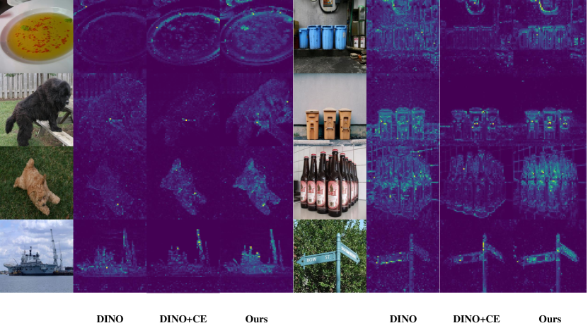
Figure 1: Visualization of Self-attention maps with the $[cls]$ token in final layers by DINO baseline, DINO + CE(with class-level supervision) and our proposed method.

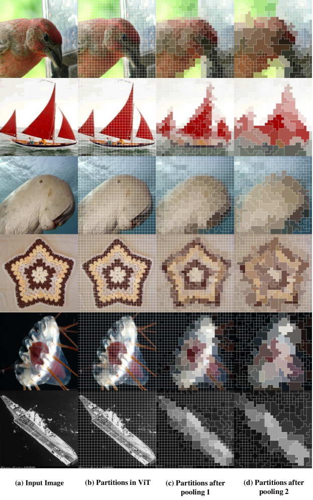
Figure 2: More visualization of tokens pooling process. After spectral tokens pooling operations, adjacent tokens with similar semantics are clustered into one. (c) and (d) shows that our clustering results are well consistent with the image’s basic structure. The pixel colors in the same cluster are averaged.

References

- [1] Arman Afrasiyabi, Jean-François Lalonde, and Christian Gagné. Mixture-based feature space learning for few-shot image classification. In Proceedings of the IEEE/CVF International Conference on Computer Vision (ICCV), pages 9041–9051, October 2021.
- [2] Marcin Andrychowicz, Misha Denil, Sergio Gomez, Matthew W Hoffman, David Pfau, Tom Schaul, Brendan Shillingford, and Nando De Freitas. Learning to learn by gradient descent by gradient descent. In Advances in neural information processing systems, pages 3981–3989, 2016.
- [3] Sungyong Baik, Janghoon Choi, Heewon Kim, Dohee Cho, Jaesik Min, and Kyoung Mu Lee. Meta-learning with task-adaptive loss function for few-shot learning. In Proceedings of the IEEE/CVF International Conference on Computer Vision, pages 9465–9474, 2021.
- [4] Luca Bertinetto, João F. Henriques, Philip H. S. Torr, and Andrea Vedaldi. Meta-learning with differentiable closed-form solvers. In 7th International Conference on Learning Representations, ICLR 2019, New Orleans, LA, USA, May 6-9, 2019. OpenReview.net, 2019.
- [5] Nicolas Carion, Francisco Massa, Gabriel Synnaeve, Nicolas Usunier, Alexander Kirillov, and Sergey Zagoruyko. End-to-end object detection with transformers. In European Conference on Computer Vision, pages 213–229. Springer, 2020.
- [6] Mathilde Caron, Ishan Misra, Julien Mairal, Priya Goyal, Piotr Bojanowski, and Armand Joulin. Unsupervised learning of visual features by contrasting cluster assignments. arXiv preprint arXiv:2006.09882, 2020.
- [7] Mathilde Caron, Hugo Touvron, Ishan Misra, Hervé Jégou, Julien Mairal, Piotr Bojanowski, and Armand Joulin. Emerging properties in self-supervised vision transformers. arXiv preprint arXiv:2104.14294, 2021.
- [8] Boyu Chen, Peixia Li, Baopu Li, Chuming Li, Lei Bai, Chen Lin, Ming Sun, Junjie Yan, and Wanli Ouyang. Psvit: Better vision transformer via token pooling and attention sharing. arXiv preprint arXiv:2108.03428, 2021.
- [9] Tianlong Chen, Yu Cheng, Zhe Gan, Lu Yuan, Lei Zhang, and Zhangyang Wang. Chasing sparsity in vision transformers:an end-to-end exploration. In Advances in Neural Information Processing Systems (NeurIPS), 2021.
- [10] Wei-Yu Chen, Yen-Cheng Liu, Zsolt Kira, Yu-Chiang Wang, and Jia-Bin Huang. A closer look at few-shot classification. In International Conference on Learning Representations, 2019.
- [11] Yinbo Chen, Zhuang Liu, Huijuan Xu, Trevor Darrell, and Xiaolong Wang. Meta-baseline: Exploring simple meta-learning for few-shot learning. In Proceedings of the IEEE/CVF International Conference on Computer Vision, pages 9062–9071, 2021.
- [12] Zhengyu Chen, Jixie Ge, Heshen Zhan, Siteng Huang, and Donglin Wang. Pareto self-supervised training for few-shot learning. In Proceedings of the IEEE/CVF Conference on Computer Vision and Pattern Recognition, pages 13663–13672, 2021.
- [13] Xiyang Dai, Yinpeng Chen, Jianwei Yang, Pengchuan Zhang, Lu Yuan, and Lei Zhang. Dynamic detr: End-to-end object detection with dynamic attention. In Proceedings of the IEEE/CVF International Conference on Computer Vision, pages 2988–2997, 2021.
- [14] Zhigang Dai, Bolun Cai, Yugeng Lin, and Junying Chen. UP-DETR: unsupervised pre-training for object detection with transformers. In IEEE Conference on Computer Vision and Pattern Recognition, CVPR 2021, virtual, June 19-25, 2021, pages 1601–1610. Computer Vision Foundation / IEEE, 2021.
- [15] Bin Dong, Fangao Zeng, Tiancai Wang, Xiangyu Zhang, and Yichen Wei. Solq: Segmenting objects by learning queries. arXiv preprint arXiv:2106.02351, 2021.
- [16] Alexey Dosovitskiy, Lucas Beyer, Alexander Kolesnikov, Dirk Weissenborn, Xiaohua Zhai, Thomas Unterthiner, Mostafa Dehghani, Matthias Minderer, Georg Heigold, Sylvain Gelly, Jakob Uszkoreit, and Neil Houlsby. An image is worth 16x16 words: Transformers for image recognition at scale. In 9th International Conference on Learning Representations, ICLR 2021, Virtual Event, Austria, May 3-7, 2021. OpenReview.net, 2021.
- [17] Nanyi Fei, Zhiwu Lu, Tao Xiang, and Songfang Huang. MELR: meta-learning via modeling episode-level relationships for few-shot learning. In 9th International Conference on Learning Representations, ICLR 2021, Virtual Event, Austria, May 3-7, 2021. OpenReview.net, 2021.
- [18] Chelsea Finn, Pieter Abbeel, and Sergey Levine. Model-agnostic meta-learning for fast adaptation of deep networks. In Proceedings of the 34th International Conference on Machine Learning-Volume 70, pages 1126–1135. JMLR. org, 2017.
- [19] Spyros Gidaris, Andrei Bursuc, Nikos Komodakis, Patrick Perez, and Matthieu Cord. Boosting few-shot visual learning with self-supervision. In The IEEE International Conference on Computer Vision (ICCV), October 2019.
- [20] Spyros Gidaris and Nikos Komodakis. Dynamic few-shot visual learning without forgetting. In Proceedings of the IEEE Conference on Computer Vision and Pattern Recognition, pages 4367–4375, 2018.
- [21] Priya Goyal, Piotr Dollar, Ross Girshick, Pieter Noordhuis, Lukasz Wesolowski, Aapo Kyrola, Andrew Tulloch, Yangqing Jia, and Kaiming He. Accurate, large minibatch sgd: Training imagenet in 1 hour. arXiv preprint arXiv:1706.02677, 2017.
- [22] Jean-Bastien Grill, Florian Strub, Florent Altché, Corentin Tallec, Pierre H. Richemond, Elena Buchatskaya, Carl Doersch, Bernardo Ávila Pires, Zhaohan Guo, Mohammad Gheshlaghi Azar, Bilal Piot, Koray Kavukcuoglu, Rémi Munos, and Michal Valko. Bootstrap your own latent - A new approach to self-supervised learning. In Hugo Larochelle, Marc’Aurelio Ranzato, Raia Hadsell, Maria-Florina Balcan, and Hsuan-Tien Lin, editors, Advances in Neural Information Processing Systems 33: Annual Conference on Neural Information Processing Systems 2020, NeurIPS 2020, December 6-12, 2020, virtual, 2020.
- [23] Ruohao Guo, Dantong Niu, Liao Qu, and Zhenbo Li. Sotr: Segmenting objects with transformers. In Proceedings of the IEEE/CVF International Conference on Computer Vision, pages 7157–7166, 2021.
- [24] Byeongho Heo, Sangdoo Yun, Dongyoon Han, Sanghyuk Chun, Junsuk Choe, and Seong Joon Oh. Rethinking spatial dimensions of vision transformers. In Proceedings of the IEEE/CVF International Conference on Computer Vision (ICCV), pages 11936–11945, October 2021.
- [25] Geoffrey Hinton. How to represent part-whole hierarchies in a neural network. arXiv preprint arXiv:2102.12627, 2021.
- [26] Geoffrey Hinton, Oriol Vinyals, and Jeff Dean. Distilling the knowledge in a neural network. arXiv preprint arXiv:1503.02531, 2015.
- [27] Muhammad Abdullah Jamal and Guo-Jun Qi. Task agnostic meta-learning for few-shot learning. In Proceedings of the IEEE Conference on Computer Vision and Pattern Recognition, pages 11719–11727, 2019.
- [28] Debesh Jha, Michael A Riegler, Dag Johansen, Pål Halvorsen, and Håvard D Johansen. Doubleu-net: A deep convolutional neural network for medical image segmentation. In 2020 IEEE 33rd International Symposium on Computer-Based Medical Systems (CBMS), pages 558–564. IEEE, 2020.
- [29] Zihang Jiang, Qibin Hou, Li Yuan, Zhou Daquan, Yujun Shi, Xiaojie Jin, Anran Wang, and Jiashi Feng. All tokens matter: Token labeling for training better vision transformers. In Thirty-Fifth Conference on Neural Information Processing Systems, 2021.
- [30] Dahyun Kang, Heeseung Kwon, Juhong Min, and Minsu Cho. Relational embedding for few-shot classification. In Proceedings of the IEEE/CVF International Conference on Computer Vision, pages 8822–8833, 2021.
- [31] Jongmin Kim, Taesup Kim, Sungwoong Kim, and Chang D Yoo. Edge-labeling graph neural network for few-shot learning. In Proceedings of the IEEE Conference on Computer Vision and Pattern Recognition, pages 11–20, 2019.
- [32] Alex Krizhevsky. Learning multiple layers of features from tiny images. University of Toronto, 2009.
- [33] Kwonjoon Lee, Subhransu Maji, Avinash Ravichandran, and Stefano Soatto. Meta-learning with differentiable convex optimization. In Proceedings of the IEEE/CVF Conference on Computer Vision and Pattern Recognition, pages 10657–10665, 2019.
- [34] Aoxue Li, Tiange Luo, Zhiwu Lu, Tao Xiang, and Liwei Wang. Large-scale few-shot learning: Knowledge transfer with class hierarchy. In Proceedings of the IEEE Conference on Computer Vision and Pattern Recognition, pages 7212–7220, 2019.
- [35] Junjie Li, Zilei Wang, and Xiaoming Hu. Learning intact features by erasing-inpainting for few-shot classification. In Thirty-Fifth AAAI Conference on Artificial Intelligence, AAAI 2021, Thirty-Third Conference on Innovative Applications of Artificial Intelligence, IAAI 2021, The Eleventh Symposium on Educational Advances in Artificial Intelligence, EAAI 2021, Virtual Event, February 2-9, 2021, pages 8401–8409. AAAI Press, 2021.
- [36] Tsung-Yi Lin, Piotr Dollár, Ross Girshick, Kaiming He, Bharath Hariharan, and Serge Belongie. Feature pyramid networks for object detection. In Proceedings of the IEEE conference on computer vision and pattern recognition, pages 2117–2125, 2017.
- [37] Ze Liu, Yutong Lin, Yue Cao, Han Hu, Yixuan Wei, Zheng Zhang, Stephen Lin, and Baining Guo. Swin transformer: Hierarchical vision transformer using shifted windows. International Conference on Computer Vision (ICCV), 2021.
- [38] Ilya Loshchilov and Frank Hutter. Fixing weight decay regularization in adam. 2018.
- [39] Jiang Lu, Pinghua Gong, Jieping Ye, and Changshui Zhang. Learning from very few samples: A survey. arXiv preprint arXiv:2009.02653, 2020.
- [40] Xu Luo, Longhui Wei, Liangjian Wen, Jinrong Yang, Lingxi Xie, Zenglin Xu, and Qi Tian. Rectifying the shortcut learning of background: Shared object concentration for few-shot image recognition. CoRR, abs/2107.07746, 2021.
- [41] Jiawei Ma, Hanchen Xie, Guangxing Han, Shih-Fu Chang, Aram Galstyan, and Wael Abd-Almageed. Partner-assisted learning for few-shot image classification. In Proceedings of the IEEE/CVF International Conference on Computer Vision, pages 10573–10582, 2021.
- [42] Puneet Mangla, Nupur Kumari, Abhishek Sinha, Mayank Singh, Balaji Krishnamurthy, and Vineeth N Balasubramanian. Charting the right manifold: Manifold mixup for few-shot learning. In The IEEE Winter Conference on Applications of Computer Vision, pages 2218–2227, 2020.
- [43] Dmitrii Marin, Jen-Hao Rick Chang, Anurag Ranjan, Anish Prabhu, Mohammad Rastegari, and Oncel Tuzel. Token pooling in vision transformers. arXiv preprint arXiv:2110.03860, 2021.
- [44] Andrew Y Ng, Michael I Jordan, and Yair Weiss. On spectral clustering: Analysis and an algorithm. In Advances in neural information processing systems, pages 849–856, 2002.
- [45] Boris N. Oreshkin, Pau Rodríguez López, and Alexandre Lacoste. TADAM: task dependent adaptive metric for improved few-shot learning. In Samy Bengio, Hanna M. Wallach, Hugo Larochelle, Kristen Grauman, Nicolò Cesa-Bianchi, and Roman Garnett, editors, Advances in Neural Information Processing Systems 31: Annual Conference on Neural Information Processing Systems 2018, NeurIPS 2018, December 3-8, 2018, Montréal, Canada, pages 719–729, 2018.
- [46] Zizheng Pan, Bohan Zhuang, Jing Liu, Haoyu He, and Jianfei Cai. Scalable vision transformers with hierarchical pooling. In Proceedings of the IEEE/CVF International Conference on Computer Vision (ICCV), pages 377–386, October 2021.
- [47] Bernhard Pfahringer, Hilan Bensusan, and Christophe G. Giraud-Carrier. Meta-learning by landmarking various learning algorithms. In Pat Langley, editor, Proceedings of the Seventeenth International Conference on Machine Learning (ICML 2000), Stanford University, Stanford, CA, USA, June 29 - July 2, 2000, pages 743–750. Morgan Kaufmann, 2000.
- [48] Siyuan Qiao, Chenxi Liu, Wei Shen, and Alan L Yuille. Few-shot image recognition by predicting parameters from activations. In Proceedings of the IEEE Conference on Computer Vision and Pattern Recognition, pages 7229–7238, 2018.
- [49] Meng Qu, Tianyu Gao, Louis-Pascal Xhonneux, and Jian Tang. Few-shot relation extraction via bayesian meta-learning on relation graphs. In International Conference on Machine Learning, pages 7867–7876. PMLR, 2020.
- [50] Yongming Rao, Wenliang Zhao, Benlin Liu, Jiwen Lu, Jie Zhou, and Cho-Jui Hsieh. Dynamicvit: Efficient vision transformers with dynamic token sparsification. In Advances in Neural Information Processing Systems (NeurIPS), 2021.
- [51] Yongming Rao, Wenliang Zhao, Zheng Zhu, Jiwen Lu, and Jie Zhou. Global filter networks for image classification. In Advances in Neural Information Processing Systems (NeurIPS), 2021.
- [52] Mengye Ren, Eleni Triantafillou, Sachin Ravi, Jake Snell, Kevin Swersky, Joshua B. Tenenbaum, Hugo Larochelle, and Richard S. Zemel. Meta-learning for semi-supervised few-shot classification. In Proceedings of 6th International Conference on Learning Representations ICLR, 2018.
- [53] Mamshad Nayeem Rizve, Salman Khan, Fahad Shahbaz Khan, and Mubarak Shah. Exploring complementary strengths of invariant and equivariant representations for few-shot learning. In Proceedings of the IEEE/CVF Conference on Computer Vision and Pattern Recognition (CVPR), pages 10836–10846, June 2021.
- [54] Olga Russakovsky, Jia Deng, Hao Su, Jonathan Krause, Sanjeev Satheesh, Sean Ma, Zhiheng Huang, Andrej Karpathy, Aditya Khosla, Michael S. Bernstein, Alexander C. Berg, and Li Fei-Fei. Imagenet large scale visual recognition challenge. Int. J. Comput. Vis., 115(3):211–252, 2015.
- [55] Jianbo Shi and Jitendra Malik. Normalized cuts and image segmentation. IEEE Transactions on pattern analysis and machine intelligence, 22(8):888–905, 2000.
- [56] Christian Simon, Piotr Koniusz, Richard Nock, and Mehrtash Harandi. Adaptive subspaces for few-shot learning. In 2020 IEEE/CVF Conference on Computer Vision and Pattern Recognition (CVPR), pages 4135–4144, 2020.
- [57] Aravind Srinivas, Tsung-Yi Lin, Niki Parmar, Jonathon Shlens, Pieter Abbeel, and Ashish Vaswani. Bottleneck transformers for visual recognition. In Proceedings of the IEEE/CVF Conference on Computer Vision and Pattern Recognition, pages 16519–16529, 2021.
- [58] Robin Strudel, Ricardo Garcia, Ivan Laptev, and Cordelia Schmid. Segmenter: Transformer for semantic segmentation. In Proceedings of the IEEE/CVF International Conference on Computer Vision (ICCV), pages 7262–7272, October 2021.
- [59] Zhiqing Sun, Shengcao Cao, Yiming Yang, and Kris M Kitani. Rethinking transformer-based set prediction for object detection. In Proceedings of the IEEE/CVF International Conference on Computer Vision, pages 3611–3620, 2021.
- [60] Flood Sung, Yongxin Yang, Li Zhang, Tao Xiang, Philip HS Torr, and Timothy M Hospedales. Learning to compare: Relation network for few-shot learning. In Proceedings of the IEEE Conference on Computer Vision and Pattern Recognition, pages 1199–1208, 2018.
- [61] Laurens Van der Maaten and Geoffrey Hinton. Visualizing data using t-sne. Journal of machine learning research, 9(11), 2008.
- [62] Oriol Vinyals, Charles Blundell, Timothy Lillicrap, koray kavukcuoglu, and Daan Wierstra. Matching networks for one shot learning. In D. D. Lee, M. Sugiyama, U. V. Luxburg, I. Guyon, and R. Garnett, editors, Advances in Neural Information Processing Systems 29, pages 3630–3638. Curran Associates, Inc., 2016.
- [63] Wenhai Wang, Enze Xie, Xiang Li, Deng-Ping Fan, Kaitao Song, Ding Liang, Tong Lu, Ping Luo, and Ling Shao. Pyramid vision transformer: A versatile backbone for dense prediction without convolutions. In IEEE ICCV, 2021.
- [64] Yandong Wen, Kaipeng Zhang, Zhifeng Li, and Yu Qiao. A discriminative feature learning approach for deep face recognition. In European conference on computer vision, pages 499–515. Springer, 2016.
- [65] Davis Wertheimer and Bharath Hariharan. Few-shot learning with localization in realistic settings. In Proceedings of the IEEE Conference on Computer Vision and Pattern Recognition, pages 6558–6567, 2019.
- [66] Haiping Wu, Bin Xiao, Noel Codella, Mengchen Liu, Xiyang Dai, Lu Yuan, and Lei Zhang. Cvt: Introducing convolutions to vision transformers. In Proceedings of the IEEE/CVF International Conference on Computer Vision (ICCV), pages 22–31, October 2021.
- [67] Jiamin Wu, Tianzhu Zhang, Yongdong Zhang, and Feng Wu. Task-aware part mining network for few-shot learning. In Proceedings of the IEEE/CVF International Conference on Computer Vision (ICCV), pages 8433–8442, October 2021.
- [68] Ziyang Wu, Yuwei Li, Lihua Guo, and Kui Jia. Parn: Position-aware relation networks for few-shot learning. In Proceedings of the IEEE International Conference on Computer Vision, pages 6659–6667, 2019.
- [69] Enze Xie, Wenhai Wang, Zhiding Yu, Anima Anandkumar, Jose M Alvarez, and Ping Luo. Segformer: Simple and efficient design for semantic segmentation with transformers. arXiv preprint arXiv:2105.15203, 2021.
- [70] Jiangtao Xie, Ruiren Zeng, Qilong Wang, Ziqi Zhou, and Peihua Li. So-vit: Mind visual tokens for vision transformer. arXiv preprint arXiv:2104.10935, 2021.
- [71] Chengming Xu, Chen Liu, Li Zhang, Chengjie Wang, Jilin Li, Feiyue Huang, Xiangyang Xue, and Yanwei Fu. Learning dynamic alignment via meta-filter for few-shot learning. In Proceedings of the IEEE Conference on Computer Vision and Pattern Recognition, 2021.
- [72] Linli Xu, Wenye Li, and Dale Schuurmans. Fast normalized cut with linear constraints. In 2009 IEEE Conference on Computer Vision and Pattern Recognition, pages 2866–2873. IEEE, 2009.
- [73] Weijian Xu, Yifan Xu, Huaijin Wang, and Zhuowen Tu. Attentional constellation nets for few-shot learning. In 9th International Conference on Learning Representations, ICLR 2021, Virtual Event, Austria, May 3-7, 2021. OpenReview.net, 2021.
- [74] Donghui Yan, Ling Huang, and Michael I Jordan. Fast approximate spectral clustering. In Proceedings of the 15th ACM SIGKDD international conference on Knowledge discovery and data mining, pages 907–916, 2009.
- [75] Shuo Yang, Lu Liu, and Min Xu. Free lunch for few-shot learning: Distribution calibration. In International Conference on Learning Representations (ICLR), 2021.
- [76] Li Yuan, Yunpeng Chen, Tao Wang, Weihao Yu, Yujun Shi, Zi-Hang Jiang, Francis E.H. Tay, Jiashi Feng, and Shuicheng Yan. Tokens-to-token vit: Training vision transformers from scratch on imagenet. In Proceedings of the IEEE/CVF International Conference on Computer Vision (ICCV), pages 558–567, October 2021.
- [77] Xiaoyu Yue, Shuyang Sun, Zhanghui Kuang, Meng Wei, Philip H.S. Torr, Wayne Zhang, and Dahua Lin. Vision transformer with progressive sampling. In Proceedings of the IEEE/CVF International Conference on Computer Vision (ICCV), pages 387–396, October 2021.
- [78] Chi Zhang, Yujun Cai, Guosheng Lin, and Chunhua Shen. Deepemd: Few-shot image classification with differentiable earth mover’s distance and structured classifiers. In IEEE/CVF Conference on Computer Vision and Pattern Recognition (CVPR), June 2020.
- [79] Chi Zhang, Henghui Ding, Guosheng Lin, Ruibo Li, Changhu Wang, and Chunhua Shen. Meta navigator: Search for a good adaptation policy for few-shot learning. In Proceedings of the IEEE/CVF International Conference on Computer Vision, pages 9435–9444, 2021.
- [80] Xueting Zhang, Debin Meng, Henry Gouk, and Timothy Hospedales. Shallow bayesian meta learning for real-world few-shot recognition. arXiv preprint arXiv:2101.02833, 2021.
- [81] Gangming Zhao, Weifeng Ge, and Yizhou Yu. Graphfpn: Graph feature pyramid network for object detection. In Proceedings of the IEEE/CVF International Conference on Computer Vision, pages 2763–2772, 2021.
- [82] Jiabao Zhao, Yifan Yang, Xin Lin, Jing Yang, and Liang He. Looking wider for better adaptive representation in few-shot learning. In Thirty-Fifth AAAI Conference on Artificial Intelligence, AAAI 2021, Thirty-Third Conference on Innovative Applications of Artificial Intelligence, IAAI 2021, The Eleventh Symposium on Educational Advances in Artificial Intelligence, EAAI 2021, Virtual Event, February 2-9, 2021, pages 10981–10989. AAAI Press, 2021.
- [83] Sixiao Zheng, Jiachen Lu, Hengshuang Zhao, Xiatian Zhu, Zekun Luo, Yabiao Wang, Yanwei Fu, Jianfeng Feng, Tao Xiang, Philip H. S. Torr, and Li Zhang. Rethinking semantic segmentation from a sequence-to-sequence perspective with transformers. In IEEE Conference on Computer Vision and Pattern Recognition, CVPR 2021, virtual, June 19-25, 2021, pages 6881–6890. Computer Vision Foundation / IEEE, 2021.
- [84] Ziqi Zhou, Xi Qiu, Jiangtao Xie, Jianan Wu, and Chi Zhang. Binocular mutual learning for improving few-shot classification. In Proceedings of the IEEE/CVF International Conference on Computer Vision, pages 8402–8411, 2021.
- [85] Xizhou Zhu, Weijie Su, Lewei Lu, Bin Li, Xiaogang Wang, and Jifeng Dai. Deformable {detr}: Deformable transformers for end-to-end object detection. In International Conference on Learning Representations, 2021.