Collision Avoidance of 3-Dimensional Objects in Dynamic Environments

Abstract

Achieving collision avoidance between moving objects is an important objective while determining robot trajectories. In performing collision avoidance maneuvers, the relative shapes of the objects play an important role. The literature largely models the shapes of the objects as spheres, and this can make the avoidance maneuvers very conservative, especially when the objects are of elongated shape and/or non-convex. In this paper, we model the shapes of the objects using suitable combinations of ellipsoids and one-sheeted/two-sheeted hyperboloids, and employ a collision cone approach to achieve collision avoidance. We present a method to construct the 3-D collision cone, and present simulation results demonstrating the working of the collision avoidance laws.

I INTRODUCTION

An important component of robot path planning is the collision avoidance problem, that is, determining a safe trajectory of a robotic vehicle so that it circumvents various obstacles in its path. When the robot and obstacles are operating in close proximity, their relative shapes can play an important role in the determination of collision avoidance trajectories. One common practice is to use polygonal approximations as bounding boxes for the shapes of the robots and obstacles. However, the polygonal approximation can lead to increased computational complexity (measured in terms of obstacle complexity, or the amount of information used to store a computer model of the obstacle, where obstacle complexity is measured in terms of the number of obstacle edges [1]). To overcome this, a common practice then is to use spherical approximations for the robots and obstacles, because of the analytical convenience of such approximations, along with the reduced information required to store a computational model of the obstacle. The obstacle avoidance conditions are then computed for the sphere as a whole.

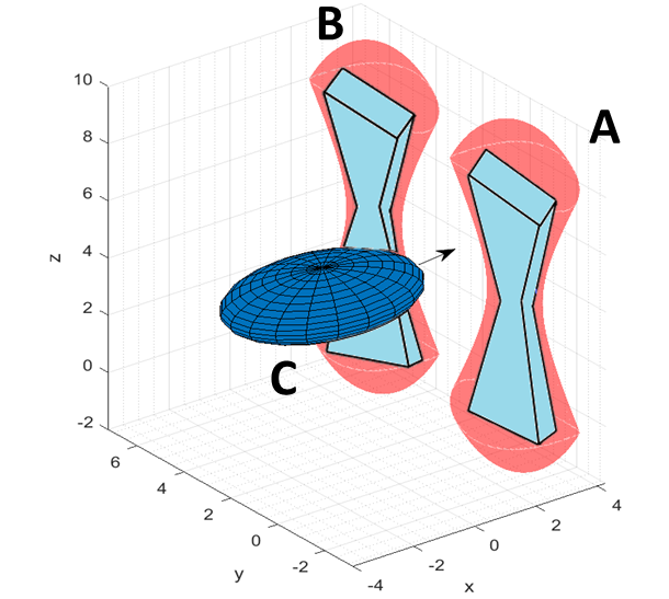
Figure 1: Elongated and/or non-convex agents in a confined space

These approximations become overly conservative in cases when an object is more elongated along one dimension compared to others. For instance, refer Fig 1 comprising three moving elongated agents. If we approximate each of $A$ and $B$ with a sphere, then these two spheres will intersect and as a consequence, $C$ will deem there is no path for it to go between $A$ and $B$, even though such a path exists. To overcome this, one can model the shapes of $A$ and $B$ using multiple smaller spheres, but this can increase the computational load. In such cases, ellipsoids have been used to serve as better approximations for the object shapes [2], [3]. For non-convex objects such as star-shaped objects  [4] however, even ellipsoidal approximations can become over conservative, because such approximations reduce the amount of available free space within which the robot trajectories can lie. In such cases, one can take recourse to non-convex bounding approximations involving a combination of ellipsoids and hyperboloids.

This paper employs a collision cone based approach to determine collision avoidance laws for moving objects having elongated, non-convex shapes. The collision cone approach, originally introduced in [5], has some similarities with the velocity obstacle approach [6] in that both approaches determine the set of velocities of the robots that will place them on a collision course with one or more obstacles. However while the velocity obstacle approach, and its many extensions [7], has been largely restricted to circles/spheres, the fact that the collision cone approach has its roots in missile guidance, enables it to determine closed form collision conditions for a larger class of object shapes [5],[8],[9]. The great benefit of obtaining analytical expressions of collision conditions is that these then serve as a basis for designing collision avoidance laws. The collision cone approach of [5] has been extensively employed in the literature (See for example, [10],[11],[12],[13],[14],[15]).

When a pair of agents have different shapes, a way to superpose the shape of one agent onto the other is to perform a Minkowski sum operation. However, this may be computationally expensive. In [16], the authors computed the collision cone between moving quadric surfaces on a plane without taking recourse to computing the Minkowski sum. In this paper, we consider a larger class of objects moving in 3-D environments and compute the 3-D collision cone between pairs of (differently shaped) 3-D objects, without computing the Minkowski sum.

II Equations of 3-D Quadric Surfaces

In this section, we present a discussion of the 3-D shapes that occur as a consequence of combining different types of quadrics. The equation of a general 3-D quadric is:

$$\begin{split}&a_{xx}x^{2}+a_{yy}^{2}+a_{zz}z^{2}+2a_{xy}xy+2a_{yz}yz+2a_{xz}xz\\ &+2b_{x}x+2b_{y}y+2b_{z}z+c_{1}=0\end{split}$$ (1)

Eqn (1) can equivalently be written in matrix form as follows:

$$\underbrace{\begin{bmatrix}x&y&z&1\end{bmatrix}}_{\bf{x}^{T}}\underbrace{\begin{bmatrix}a_{xx}&a_{xy}&a_{x}&b_{x}\\ a_{xy}&a_{yy}&a_{yz}&b_{y}\\ a_{xz}&a_{yz}&a_{zz}&b{z}\\ b_{x}&b_{y}&b_{z}&c_{1}\end{bmatrix}}_{\bf{Q}}\underbrace{\begin{bmatrix}x\\ y\\ z\\ 1\end{bmatrix}}_{\bf{x}} = 0$$ (2)

When $det(\mathbf{Q})<0$, (1) represents an ellipsoid or a one-sheeted hyperboloid, and when $det(\mathbf{Q})>0$, it represents a two-sheeted hyperboloid. We refer to the matrices corresponding to an ellipsoid, one-sheeted hyperboloid and two-sheeted hyperboloid as $\mathbf{Q_{e}}$, $\mathbf{Q_{h1}}$ and $\mathbf{Q_{h2}}$, respectively. Please also note that in this paper, vectors are represented in lowercase boldface, and matrices in uppercase boldface.

We now proceed towards determination of equations of surfaces comprised of different combinations of the above quadric surfaces.

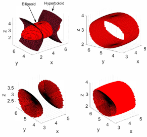
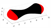
Figure 2: a) Ellipsoid and Hyperboloid b) Ellipsoid delimited by Hyperboloid c) Hyperboloid delimited by Ellipsoid d) Biconcave Ellipsoid e) Biconvex Hyperboloid

We define the interior of a quadric as the region which includes the center of the quadric and the exterior as the complement of the interior. Accordingly, the regions $\{x:\mathbf{x}^{T}\mathbf{Q}_{e}\mathbf{x}<0$} and $\{x:\mathbf{x}^{T}\mathbf{Q}_{h1}\mathbf{x}<0\}$ represent, respectively, the interiors of the ellipsoid corresponding to $Q_{e}$, and the one-sheeted hyperboloid corresponding to $Q_{h1}$. On the other hand, the region $\{x:\mathbf{x}^{T}\mathbf{Q}_{h2}\mathbf{x}<0$} represents the exterior of the two-sheeted hyperboloid corresponding to $Q_{h2}$. We now use these properties to construct surfaces that comprise combinations of two intersecting quadrics. In constructing these combinations, we employ the phrase “delimited”, which means “having fixed boundaries or limits”.

Consider an intersecting ellipsoid and two-sheeted hyperboloid, as shown in Fig 2a. Then, we define the surface of an Ellipsoid Delimited by a Hyperboloid (EDH) as follows:

$$\mathbf{x}^{T}\mathbf{Q_{e}}\mathbf{x}=0,\ \text{subject to:}\bf{x}^{T}\bf{Q}_{h2}\bf{x}>0$$ (3)

The above equation states that the surface of the EDH comprises those points on the surface of the ellipsoid that are not present inside the two-sheeted hyperboloid. The surface of an EDH is shown in Fig 2b.

We next define the surface of a two-sheeted Hyperboloid Delimited by an Ellipsoid (HDE) as follows:

$$\mathbf{x}^{T}\mathbf{Q_{h2}}\mathbf{x}=0,\ \text{subject to:}\bf{x}^{T}\bf{Q}_{e}\bf{x}<0$$ (4)

The above equation states that the surface of a HDE comprises those points on the surface of a two-sheeted hyperboloid that are present inside the ellipsoid. Such a HDE is shown in Fig 2c.

We can combine (3) and (4) to determine a surface composed of an EDH and a HDE. This is shown in Fig 2d, and is mathematically represented as:

$$K_{1}\mathbf{x}^{T}\mathbf{Q_{e}}\mathbf{x}+K_{2}\mathbf{x}^{T}\mathbf{Q_{h2}}\mathbf{x}=0\textrm{, where}$$ (5)

$$K_{1}=\begin{cases}1\ if\ \{x:\mathbf{x}^{T}\mathbf{Q_{h2}}\mathbf{x}>0\}\\ 0\ \textrm{otherwise}\end{cases},K_{2}=\begin{cases}1\ if\ \{x:\mathbf{x}^{T}\mathbf{Q_{e}}\mathbf{x}<0\}\\ 0\ \textrm{otherwise}\end{cases}$$

With some abuse of terminology, we refer to the above as a biconcave ellipsoid. Finally, we combine a one-sheeted hyperboloid and an ellipsoid. Its mathematical representation is as follows:

$$K_{1}\mathbf{x}^{T}\mathbf{Q_{e}}\mathbf{x}+K_{2}\mathbf{x}^{T}\mathbf{Q_{h1}}\mathbf{x}=0\textrm{, where}$$ (6)

$$K_{1}=\begin{cases}1\ if\ \{x:\mathbf{x}^{T}\mathbf{Q_{h1}}\mathbf{x}<0\}\\ 0\ \textrm{otherwise}\end{cases},K_{2}=\begin{cases}1\ if\ \{x:\mathbf{x}^{T}\mathbf{Q_{e}}\mathbf{x}<0\}\\ 0\ \textrm{otherwise}\end{cases}$$

This is shown in Fig 2e. With some abuse of terminology, we refer to this as a biconvex hyperboloid. We note that by combining an ellipsoid with multiple hyperboloids at different orientations, one can also approximate star-shaped objects.

III 3D engagement geometry

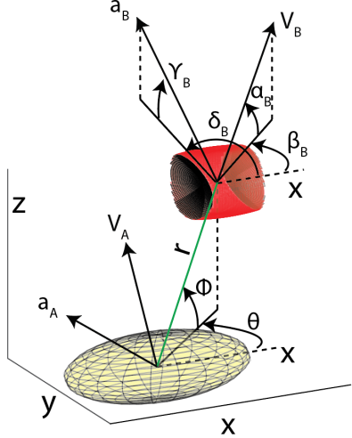
Figure 3: Engagement Geometry between two objects

Fig 3 shows the engagement geometry between two objects $A$ and $B$. While the figure shows $A$ and $B$ to be an ellipsoid and a biconcave ellipsoid, they could in principle be any pair of objects discussed in Section II. $A$ and $B$ are moving with speeds $V_{A}$ and $V_{B}$, respectively, at heading angle pairs of $(\beta_{A},\alpha_{A})$, and $(\beta_{B},\alpha_{B})$ respectively. Here, $\beta_{A}$ and $\alpha_{A}$ represent, respectively, the azimuth and elevation angles of the velocity vector of $A$, and a corresponding definition holds for $\beta_{B}$ and $\alpha_{B}$. $r$ represents the distance between the centers of $A$ and $B$, and $(\theta,\phi)$ represents the azimuth-elevation angle pair of line joining the center of $A$ and $B$. The control input of $A$ is its lateral accelerations $a_{A}$, which acts normal to the velocity vector of $A$ at an azimuth-elevation angle pair of ($\delta_{A},\gamma_{A}$). A corresponding definition holds for the lateral acceleration $a_{B}$ of $B$. $V_{r},V_{\theta},V_{\phi}$ represent the mutually orthogonal components of the relative velocity of $B$ with respect to $A$, where $V_{r}$ acts along the line joining the centers of $A$ and $B$. The kinematics governing the engagement geometry are characterized by the following:

$$\begin{split}&\dot{r}=V_{r},\,\,\dot{\theta}=V_{\theta}/(r\cos\phi),\,\,\dot{\phi}=V_{\phi}/r\\ &\dot{V}_{\theta}=(-V_{\theta}V_{r}+V_{\theta}V_{\phi}\tan\phi)/r-(\cos\gamma_{A}\sin(\delta_{A}-\theta))a_{A}\\ &\quad\quad+(\cos\gamma_{B}\sin(\delta_{B}-\theta))a_{B}\\ &\dot{V}_{\phi}=(-{V_{\theta}}{V_{r}}-V_{\theta}^{2}\tan{\phi})/{r}+(\cos{\gamma_{A}}\sin{\phi}\cos{(\delta_{A}-\theta)}\\ &-\sin{\gamma_{A}}\cos{\phi})a_{A}-(\cos{\gamma_{B}}\sin{\phi}\cos{(\delta_{B}-\theta)}-\sin{\gamma_{B}}\cos{\phi})a_{B}\\ &\dot{V}_{r}=(V_{\theta}^{2}+V_{\phi}^{2})/{r}-(\cos{\gamma_{A}}\cos{\phi}\cos{(\delta_{A}-\theta)}+\sin{\gamma_{A}}\sin{\phi})a_{A}\\ &+(\cos{\gamma_{B}}\cos{\phi}\cos{(\delta_{B}-\theta)}+\sin{\gamma_{B}}\sin{\phi})a_{B}\end{split}$$ (7)

IV Collision Cone Computation

IV-A 2D Collision Cone for arbitrarily shaped objects

Refer Fig 4, which shows two arbitrarily shaped objects $A$ and $B$ moving with velocities $V_{A}$ and $V_{B}$, respectively. The lines $Q_{1}Q_{2}$ and $R_{1}R_{2}$ form a sector with the property that this represents the smallest sector that completely contains $A$ and $B$ such that $A$ and $B$ lie on opposite sides of the point of intersection $O$. Let $\hat{V}_{r}$ and $\hat{V}_{\theta}$ represent the relative velocity components of the angular bisector of this sector and $V_{r}$ and $V_{\theta}$ represents the relative velocity components of line-of-sight, they are related as follows:

$$\begin{bmatrix}\hat{V}_{r}\\ \hat{V}_{\theta}\end{bmatrix}=\begin{bmatrix}\cos\left({\theta}-\theta_{b}\right)&\sin\left({\theta}-\theta_{b}\right)\\ -\sin\left({\theta}-\theta_{b}\right)&\cos\left({\theta}-\theta_{b}\right)\end{bmatrix}\begin{bmatrix}V_{r}\\ V_{\theta}\end{bmatrix}$$ (8)

As demonstrated in [5], $A$ and $B$ are on a collision course if their relative velocities belong to a specific set. This set is encapsulated in a quantity $y$ defined as follows:

$$y=\dfrac{\hat{V}_{\theta}^{2}}{\left(\hat{V}_{\theta}^{2}+\hat{V}_{r}^{2}\right)}-\sin^{2}\left({\dfrac{\psi}{2}}\right)$$ (9)

The collision cone is defined as the region in the $(\hat{V}_{\theta},\hat{V}_{r})$ space for which $y<0$, $\hat{V}_{r}<0$ is satisfied. Thus, any relative velocity vector satisfying this condition lies inside the collision cone. The condition corresponding to $y=0$ and $\hat{V}_{r}<0$ defines the boundaries of the collision cone and any relative velocity vector satisfying this condition is aligned along the boundary of the cone.

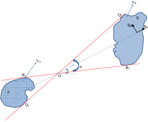
Figure 4: Engagement geometry between arbitrarily shaped objects

A challenge in computing the collision cone for arbitrarily shaped objects is in the computation of the sector enclosing the objects $A$ and $B$ (shown in Fig 4), and determination of the angle $\psi$. Note that as $A$ and $B$ move, the angle $\psi$ changes with time. An iterative method to determine $\psi$ for arbitrarily shaped objects using the concept of conical hulls was presented in [17]. In [16], an alternative, computationally light method to compute $\psi$ for objects modeled by 2-D quadric surfaces was presented. A method to compute 3-D collision cones for generic objects was presented in [9]. In this paper, we extend the results from [5], [9] and [16], to present a computationally inexpensive method to determine the 3-D collision cones corresponding to the objects discussed in Section II.

IV-B 3D Collision Cone between two Ellipsoids

We consider the scenario where $A$ and $B$ are ellipsoids. Let $\mathbf{Q_{eA}}$ and $\mathbf{Q_{eB}}$ represent the respective matrices corresponding to these ellipsoids. A $3D$ collision cone between $A$ and $B$ can be generated by first computing the $2D$ collision cones on several planes, and subsequently merging these $2D$ cones to get a combined cone in $3D$. Without loss of generality, we stipulate that all planes contain the line joining the centers of $A$ and $B$, and each successive plane is generated by rotating the preceding plane about this line.

Let the centers of $A$ and $B$ be $(A_{x},\ A_{y},\ A_{z})$ and $(B_{x},\ B_{y},\ B_{z})$, respectively. Let $\mathbf{r}$ represent the vector joining these centers. Let $\mathbf{P_{j}}$ represent the $j^{th}$ plane, where $j\in\big{\{}1,2,\ldots,n\big{\}}$, and $n$ is the number of planes.

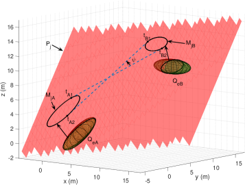
Figure 5: Procedure to construct 3D collision cone between two ellipsoids

Refer Fig 5, which shows one such plane. Let $\mathbf{R_{xj}}$ and $\mathbf{R_{yj}}$ be two mutually orthogonal unit vectors on this plane. Here, we choose $\mathbf{R_{yj}}=\mathbf{r}$ and $\mathbf{R_{xj}}$ orthogonal to it, on that plane. Define a matrix corresponding to the plane as follows:

$$\mathbf{P_{j}}=\begin{bmatrix}\mathbf{R_{xj}}&\mathbf{R_{yj}}&[A_{x},\ A_{y},\ A_{z}]^{T}\\ 0&0&1\end{bmatrix}$$

The intersection of the plane $P_{j}$ with the two ellipsoids $A$ and $B$, will produce two ellipses. The matrices $\mathbf{M_{jA}}$ and $\mathbf{M_{jB}}$ corresponding to these ellipses are found as follows:

$$\mathbf{M_{jA}}=\mathbf{P_{j}}^{T}\mathbf{Q_{eA}}\mathbf{P_{j}},~{}~{}~{}\mathbf{M_{jB}}=\mathbf{P_{j}}^{T}\mathbf{Q_{eB}}\mathbf{P_{j}}$$ (10)

We then obtain the duals of these two ellipses as:

$$\mathbf{C_{1}}=\mathbf{M_{jA}}^{-1},~{}~{}~{}\mathbf{C_{2}}=\mathbf{M_{jB}}^{-1}$$ (11)

Next, we compute the collision cone between $\mathbf{M_{jA}}$ and $\mathbf{M_{jB}}$. For that, we compute the common tangents to these two ellipses, using algorithm IV-B. This algorithm provides the points of tangency $t_{A1},t_{A2}$ that lie on $\mathbf{M_{jA}}$ and $t_{B1},t_{B2}$ that lie on $\mathbf{M_{jB}}$ (Please see Fig 5 for an illustration).

   1 Common tangents to two ellipses

 

1:// Given two matrices $\mathbf{C_{1}}$ and $\mathbf{C_{2}}$

2:// Determine the degenerate conics

3:$[U,\textbf{t}]=eig(\mathbf{C_{2}}^{-1}\mathbf{C_{1}}$) $\triangleright$ $\mathbf{U}=[\mathbf{u_{1}}\ \mathbf{u_{2}}\ \mathbf{u_{3}}],\ \mathbf{t}=[t_{1},\ t_{2},\ t_{3}]^{T}$

4:// Perform Projective transformation of degenerate conic by $\mathbf{U}$

5:$\mathbf{L}_{i}=\mathbf{U}^{T}(\mathbf{C_{1}}-\mathbf{t}_{i}\mathbf{C_{2}})U$ for $i=1,2$

6:// Find one of the intersection point of these projected degenerate conics

7:$x=\sqrt{-\dfrac{\mathbf{L}_{2}(3,3)}{\mathbf{L}_{2}(1,1)}},\ y=\sqrt{-\dfrac{\mathbf{L}_{1}(3,3)}{\mathbf{L}_{1}(2,2)}}$

8:// Find all the tangent lines in projected coordinate system

9:$\mathbf{S}=\begin{bmatrix}x&y&1\\ -x&-y&1\\ -x&y&1\\ x&-y&1\end{bmatrix}$

10:// Deproject the solution to homogeneous system

11:$\mathbf{S}=\mathbf{S}\mathbf{U}^{T}$

12:// Define the centers of $\mathbf{M_{jA}}$ and $\mathbf{M_{jB}}$

13:$\mathbf{d_{1}}=\mathbf{C_{1}}[0\ 0\ 1]^{T},\ \mathbf{d_{1}}=\mathbf{d_{1}}/\mathbf{d_{1}}(3)$

14:$\mathbf{d_{2}}=\mathbf{C_{2}}[0\ 0\ 1]^{T},\ \mathbf{d_{2}}=\mathbf{d_{2}}/\mathbf{d_{2}}(3)$

15:// Determine which of the solutions are the inner tangents by using the property that two centers of the ellipses lie on opposite sides of the inner tangents. Defining a boolean vector

16:$bool=(\mathbf{Sd}_{1})\odot(\mathbf{Sd}_{2})<0$ $\triangleright$ $\odot$ is Hadamard product

17:// Eliminating the indices of $s$ marked as false in $bool$

18:$\mathbf{S}=\mathbf{S}(bool)$

19:// Determine the homogeneous coordinates of tangent points on ellipses $\mathbf{M_{jA}}$ and $\mathbf{M_{jB}}$

20:$t_{A}=\mathbf{C_{1}S}$, $t_{B}=\mathbf{C_{2}S}$

 

Note that $t_{A}$, $t_{B}$ $\in$ $\mathbf{R}^{3\times 2}$ where each column denotes the homogeneous coordinates of each point of tangency. After obtaining these points of tangency, we obtain the tangent lines passing through these points and then find collision cone parameters $\psi$ and $\theta_{b}$ on that particular plane. Henceforth, all the projected $2D$ states on a plane are marked by a subscript $P$. Thus, $\psi_{Pj}$ and $\theta_{bPj}$ represent the values of $\psi$ and $\theta_{b}$ on plane $\mathbf{P_{j}}$.

Projection of $3D$ relative states into the $2D$ plane

The final step of computing the $3D$ collision cone involves computing the projection of the $3D$ states of the objects $A$ and $B$ on each plane $P_{j},j=\{1,\ldots,n\}$. Since by construction, all the planes contain the vector $\mathbf{r}$, so the length of the $3D$ vector $r$ is equal to its corresponding 2D projection, that is $r=r_{p}$. $\theta_{p}$ is LOS angle from $\mathbf{d_{1}}$ to $\mathbf{d_{2}}$. Also, the relative velocity component along $\mathbf{r}$ in 3D (that is, $V_{r}$) will be equal to the relative velocity along LOS in 2D (that is, $V_{rp}$) and the $2D$ relative velocity perpendicular to $\mathbf{r}$, $V_{\theta p}$ acts along the direction of $\mathbf{R_{xj}}$. Defining $V$ as the relative velocity vector between $A$ and $B$ as $\mathbf{V}=\mathbf{V}_{B}-\mathbf{V}_{A}$, $\hat{\mathbf{V}}_{\theta}=\mathbf{R_{xj}}$ as the unit vector along $V_{\theta 2D}$, we get the following expressions for the projected $2D$ relative velocity components: 1) $V_{rp}=V_{r},\,2)V_{\theta p}=(\mathbf{V}-{\mathbf{V}}_{r})\cdot\hat{\mathbf{V}}_{\theta}$ Then using (9), we can compute collision cone in $2D$. We repeat this process over all the $n$ planes to ultimately obtain $3D$ collision cone.

Influence of $n$ on accuracy of 3D cone:

We note that by increasing the number of planes $n$, we can increase the accuracy of the collision cone, but this increases the computation time. The proper choice of $n$ depends on the computational resources available and accuracy desired. To evaluate the effect of $n$ on accuracy, a Monte Carlo simulation of $10,000$ different engagement geometries of two ellipsoids was performed, and for each engagement, the 3-D collision cone was computed for varying values of $n$. The cross-sectional area of the 3-D collision cone was computed in each case and this was used to determine the numerical accuracy as follows. The 3-D cone obtained with $n=360$ was treated as the truth model and the difference between the cross-sectional area of this cone, with the cone obtained using other values of $n$ is shown in Fig 6 (the error is expressed as a fraction). As seen in Fig 6, the error decreases rapidly with increasing $n$, and has an upper bound of $2/n$. This shows that a small number of planes can be used to compute the 3D collision cone with a relatively small error.

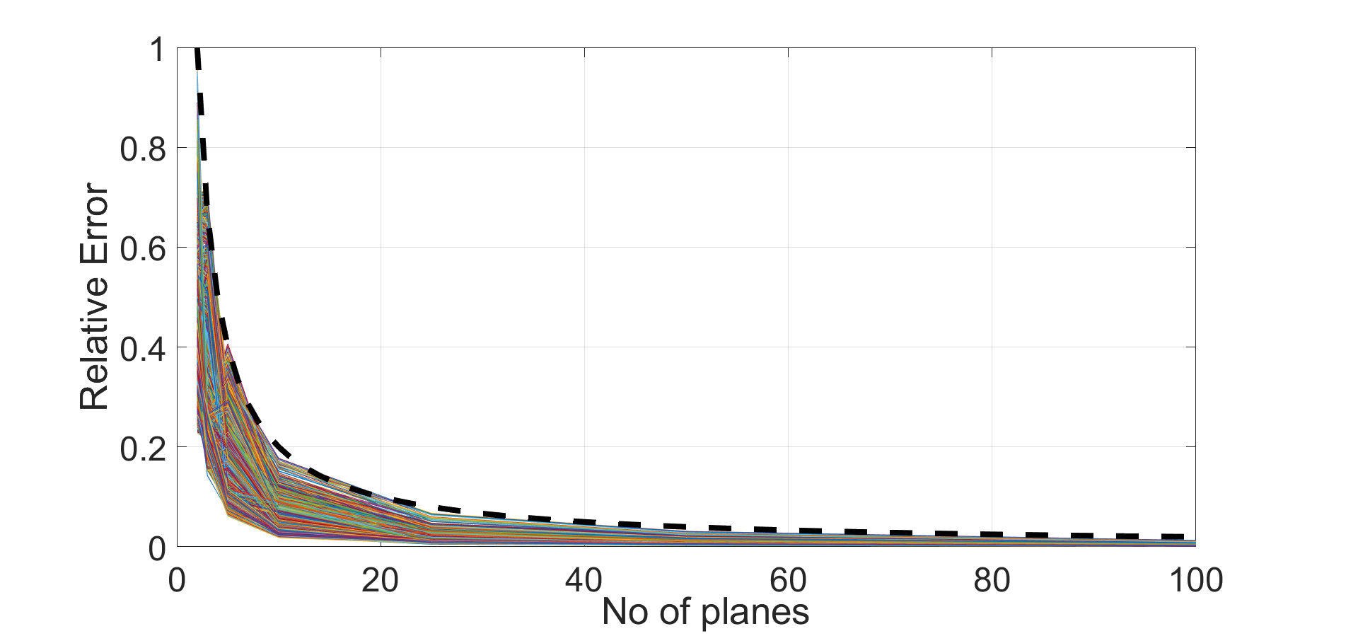
Figure 6: Plot of relative error vs. no. of planes

IV-C 3D Collision cone between an ellipsoid and a biconcave ellipsoid

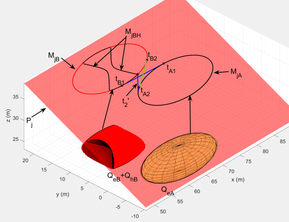
Figure 7: 3D collision cone between an ellipsoid and a biconcave ellipsoid

We next consider the scenario where $A$ is an ellipsoid $A$ and $B$ is a biconcave ellipsoid. Let the matrix corresponding to $A$ be $(\mathbf{Q_{eA}})$, and those corresponding to $B$ be $(\mathbf{Q_{eB}})$ and Hyperboloid $(\mathbf{Q_{hB}})$. To compute collision cone in this case, we take the planar cross-sections of the two objects similar to the case of two ellipsoids. First, we consider the engagement between $\mathbf{Q_{eA}}$ and $\mathbf{Q_{eB}}$ and define $C_{1}$ and $C_{2}$ on several planar cross-sections. Refer Fig 7, which shows the cross-sections on one such plane $\mathbf{P_{j}}$.

We use (11) and find the points of tangency on $\mathbf{M_{jA}}$ and $\mathbf{M_{jB}}$ using algorithm IV-B. This will give us two points of tangency on each of $\mathbf{M_{jA}}$ (say $t_{A1}$ and $t_{A2}$) and $\mathbf{M_{jB}}$ (say $t_{B1}$ and $t_{B2}$). We use these to define two candidate tangent lines (say $t_{1}$ and $t_{2}$) passing through the pairs of points $(t_{A1},t_{B1})$ and $(t_{A2},t_{B2})$ respectively, and then check if $t_{1}$ and $t_{2}$ are valid tangent lines.

Note that the planar cross-section of a biconcave ellipsoid can be either an ellipse or a combination of ellipse and hyperbola (say, a biconcave ellipse). If the planar cross section is an ellipse, then the candidate solutions $t_{1}$ and $t_{2}$ can be accepted as the valid solution on that plane. However if that is not the case, then we check if the points $t_{B1}$ and $t_{B2}$ lie on the biconcave ellipse. For this, we first determine the equation of the hyperbola on the plane $\mathbf{P_{j}}$ as:

$$\mathbf{M_{jBH}}=\mathbf{P_{j}}^{T}\mathbf{Q_{eH}}\mathbf{P_{j}}$$ (12)

and then check if $\mathbf{t_{Bi}}^{T}\mathbf{M_{jBH}}\mathbf{t_{Bi}}<0,\,i=1,2$

If either $t_{B1}$ and $t_{B2}$ satisfy the above equation then the corresponding tangent lines can be accepted as valid common tangents. The ones that do not satisfy the above equation need to be replaced by a new line tangent to $\mathbf{M_{jA}}$ passing through one of the corner points $(L,M,N,P)$ of the biconcave ellipse. Note that the corner points can be obtained using algorithm IV-B by taking $\mathbf{C_{1}}=\mathbf{P_{j}^{T}Q_{eB}P_{j}}$ and $\mathbf{C_{2}}=\mathbf{P_{j}^{T}Q_{eH}P_{j}}$. After performing steps 1-5, we can obtain the desired corner points in the homogeneous system as $s$. To draw tangents from a corner point to $A$ we use a computationally efficient approach presented in [16]. To proceed, we draw two tangents from each of the corner points to $\mathbf{M_{jA}}$. These tangent lines would be considered valid if: i) the centers of $\mathbf{M_{jA}}$ and $\mathbf{M_{jB}}$ lie on opposite sides of each line, and ii) All the four corner lie on the same side of each line. We eliminate the candidates that do not satisfy these properties, and this will leave us with two inner common tangents from the four corner points to $\mathbf{M_{jA}}$. Call these $t_{1}^{\prime}$ and $t_{2}^{\prime}$. If both $t_{1}$ and $t_{2}$ computed above are invalid then $t_{1}^{\prime}$ and $t_{2}^{\prime}$ can be accepted as the inner common tangents. However, if only one of them is invalid then that invalid tangent line should be replaced by $t_{1}^{\prime}$ or $t_{2}^{\prime}$, as the case may be. We finally use these computed tangents to calculate $\psi_{p}$ and $\theta_{bp}$ in (9) to compute the collision cone. A similar set of steps can be used to compute the collision cone between an ellipsoid and a biconvex hyperboloid.

IV-D 3D Collision Cone between an ellipsoid and an arbitrarily shaped object

Let $A$ be an ellipsoid $(\mathbf{Q_{eA}})$ and $B$ represent an obstacle of arbitrary shape that cannot be represented analytically. Assume that $A$ is equipped with multiple lidars and the point clouds from these lidars are fused using the Iterative Closest Point (ICP) algorithm [18]. This 3D point cloud can then be used to determine the intersection of $B$ with a plane passing through the center of $A$ and $B$. Similar to the case of two ellipsoids, we obtain multiple planar cross-sections of $A$ and $B$. Planar cross-sections of $A$ corresponding to ellipse $\mathbf{M_{jA}}$ can be determined using (10). However planar cross-sections of $B$ cannot be determined because it’s shape is unknown and in fact, the only available knowledge of $B$ is of that portion of $B$ which can be viewed by the lidars on $A$. Let $\mathbf{M_{jB}}$ represent the portion of the planar cross section of $B$, which is visible from the lidars on $A$. A schematic is shown in Fig 8.

To obtain collision cone on that plane, we need to find the common tangents to $\mathbf{M_{jA}}$ and $\mathbf{M_{jB}}$. For this, we first draw four tangents, two from each of the extreme ends of $\mathbf{M_{jB}}$ to $\mathbf{M_{jA}}$. For each such line, we check if the centers of $\mathbf{M_{jA}}$ and $\mathbf{M_{jB}}$ lie on opposite sides of the line, and additionally, all points of $\mathbf{M_{jB}}$ lie on the same side. If these criteria are satisfied by any two lines, then these correspond to the desired common tangents and we can proceed towards computation of collision cone. Otherwise, we perform a search across the points of $\mathbf{M_{jB}}$ (starting from its extreme ends and moving towards the middle), and repeat this process until we find two common tangent lines. We note that the points on the boundary of $\mathbf{M_{jB}}$ can be down-sampled to decrease the computation time. In most of the cases, the common tangents would pass through the points that are closer to the extreme ends of $\mathbf{M_{jB}}$, and so this algorithm would be able to find the solution in a few iterations. We point out that since this algorithm involves a search process, it will be computationally more expensive then the one used for quadrics in the preceding sections, but will still be computationally efficient.

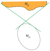
Figure 8: Planar section of an ellipsoid and an arbitrary object

V Collision Avoidance Acceleration

From (8) and (9), we obtain the collision cone function $y_{p}$ for each plane so that it is now written in terms of the $2D$ states of the selected plane using the subscript $p$ as follows:

$$y_{p}=\dfrac{\Big{[}\begin{multlined}{V}_{\theta_{p}}^{2}\cos^{2}({\theta_{p}}-\theta_{bp})+V_{r}^{2}\sin^{2}(\theta_{p}-\theta_{bp})\\ +2V_{r}V_{\theta_{p}}\cos(\theta_{p}-\theta_{bp})\sin(\theta_{p}-\theta_{pb})\end{multlined}{V}_{\theta_{p}}^{2}\cos^{2}({\theta_{p}}-\theta_{bp})+V_{r}^{2}\sin^{2}(\theta_{p}-\theta_{bp})\\ +2V_{r}V_{\theta_{p}}\cos(\theta_{p}-\theta_{bp})\sin(\theta_{p}-\theta_{pb})\Big{]}}{V_{rp}^{2}+V_{\theta p}^{2}}-\sin^{2}\left({\dfrac{\psi_{p}}{2}}\right)$$ (13)

The set of heading angles of $A$ satisfying $y_{p}<0,\hat{V}_{rp}<0$ on each plane are obtained, and then combined to get the $3D$ collision cone for that engagement. If the velocity vector of $A$ lies inside the collision cone, then $A$ is on a collision course with $B$, and needs to apply a suitable lateral acceleration $a_{A}$ to drive steer its velocity vector out of the collision cone. We present a discussion on the choice of the avoidance plane (on which $a_{A}$ is to be applied), followed by analytical expressions for the lateral acceleration law required for collision avoidance.

V-A Selection of Collision Avoidance Plane

From the computed $3D$ collision cone, we take a $2D$ slice on a chosen plane, and then compute the lateral acceleration for avoidance on that plane. We note that the choice of this plane can vary from one time instant to the next, and this is particularly true in dynamic environments and scenarios where the cross section of the 3D cone is not circular, or is non-convex (such as those discussed in this paper). There can be several ways to choose this plane. For instance, we can choose a plane on which the heading angle of the agent is closest to the boundary of the cone. Such a choice ensures that the angular deviation in the velocity vector of the vehicle (to get out of the cone) is small. In windy environments, the avoidance plane can be chosen such that the directions of the applied lateral acceleration and the wind vector are not directly opposed to each other. Other alternatives also exist.

V-B Collision Avoidance Law

On the chosen avoidance plane, $A$ needs to apply a suitable lateral acceleration $a_{A}$ to drive $y_{p}$ to a reference value $w\geq 0$, as this will be equivalent to steering its velocity vector out of the collision cone. We employ dynamic inversion to determine this lateral acceleration. Differentiating (13), we obtain the dynamic evolution of $y_{p}$ as follows:

$$\begin{split}\dot{y}_{p}&=\frac{\partial y_{p}}{\partial\theta_{bp}}\dot{\theta_{bp}}+\frac{\partial y_{p}}{\partial\theta_{p}}\dot{\theta_{p}}+\frac{\partial y_{p}}{\partial V_{\theta p}}\dot{V}_{\theta p}+\frac{\partial y_{p}}{\partial V_{rp}}\dot{V}_{rp}+\frac{\partial y_{p}}{\partial\psi_{p}}{\dot{\psi_{p}}}\end{split}$$ (14)

Define an error quantity $z_{p}(t)=y_{p}(t)-w$. Taking $w$ as a constant $\forall t$, we seek to determine $a_{lat,A}$ which will ensure the error $z_{p}(t)$ follows the dynamics $\dot{z}_{p}=-Kz_{p}$ where $K>0$ is a constant. This in turn causes the quantity $y$ to follow the dynamics $\dot{y}_{p}=-K(y_{p}-w)$. Note that all the partial derivatives of $y_{p}$ can be computed analytically from (13). While the state kinematic equations are given in (7), we however do not have analytical expressions of $\dot{\theta}_{bp}$ and $\dot{\psi}_{p}$ and these will have to be synthesized numerically.

Non-cooperative Collision Avoidance: Here, the onus is on $A$ to apply a lateral acceleration to steer its velocity vector out of the collision cone, and $B$ does not cooperate. Substituting partial derivatives and state derivatives in (14) and assuming $a_{B}=0$, we get an expression for $a_{A}$ as:

$$a_{A}=-(V_{rp}^{2}+V_{\theta p}^{2})\frac{N_{1}+N_{2}}{D_{1}D_{2}}$$ (15)

where, the quantities $N_{1}$, $N_{2}$, $D_{1}$, $D_{2}$ are as follows:

$$\begin{split}N_{1}&=(V_{rp}^{2}+V_{\theta p}^{2})(2K(w-y_{p})+\dot{\psi_{p}}\sin(\psi_{p})),\,N_{2}=2\dot{\theta_{b}}_{p}D_{1}\\ D_{1}&=2V_{rp}V_{\theta p}\cos(2(\theta_{p}-\theta_{bp}))+(V_{rp}^{2}-V_{\theta p}^{2})\sin(2(\theta_{p}-\theta_{bp}))\\ D_{2}&=2\left(V_{rp}\cos(\alpha_{pA}-\theta_{p})+V_{\theta p}\sin(\alpha_{pA}-\theta_{p})\right)\end{split}$$

Cooperative Collision Avoidance: Here, $A$ and $B$ cooperate with one other in applying suitable lateral accelerations so that they jointly steer their velocity vectors out of the collision cone. Assume that $\mu$ represents the acceleration ratio, that is, $\mu=a_{B}/a_{A}$. Substituting partial derivatives and state derivatives in (14), we get equations for $a_{A}$, $a_{B}$ as:

$$\begin{split}&0.5a_{A}\ D_{1}+a_{B}\ N_{3}=-\frac{N_{1}+\dot{\theta}_{bp}D_{1}(V_{rp}^{2}+V_{\theta p}^{2})}{D_{1}},\text{where}\\ &N_{3}=-(V_{rp}\cos(\alpha_{pB}-\theta_{p})-V_{\theta p}\sin(\alpha_{pB}-{\theta p}))\end{split}$$ (16)

Using the acceleration ratio $\mu$, the above leads to the following accelerations:

$$\begin{split}a_{A}=-\frac{N_{1}+\dot{\theta}_{bp}D_{1}(V_{rp}^{2}+V_{\theta p}^{2})}{D_{1}(0.5D_{1}+\mu N_{3})},\ a_{B}=\mu a_{A}\end{split}$$ (17)

Computation of Direction of Acceleration Vectors : These computed $a_{A}$ and $a_{B}$ are applied at angles of $(\alpha_{pA}+\pi/2)$ and $(\alpha_{pB}+\pi/2)$, respectively, on the selected plane. Here, $\alpha_{pA}$ and $\alpha_{pB}$ represent the heading angles of $A$ and $B$ on that plane. In $3D$, the direction of the applied acceleration is as follows:

$$\hat{a}_{i} = \mathbf{P_{j}}\ [\cos(\pi/2+\alpha_{pi})\ \sin(\pi/2+\alpha_{pi})\ 0]^{T}$$

$$\delta_{i} = \tan^{-1}\left(\frac{\hat{a}_{i}(2)}{\hat{a}_{i}(1)}\right),\,\gamma_{i}=\sin^{-1}\left(\frac{\hat{a}_{i}(3)}{\|\hat{a}_{i}\|}\right),\,i=A,B$$

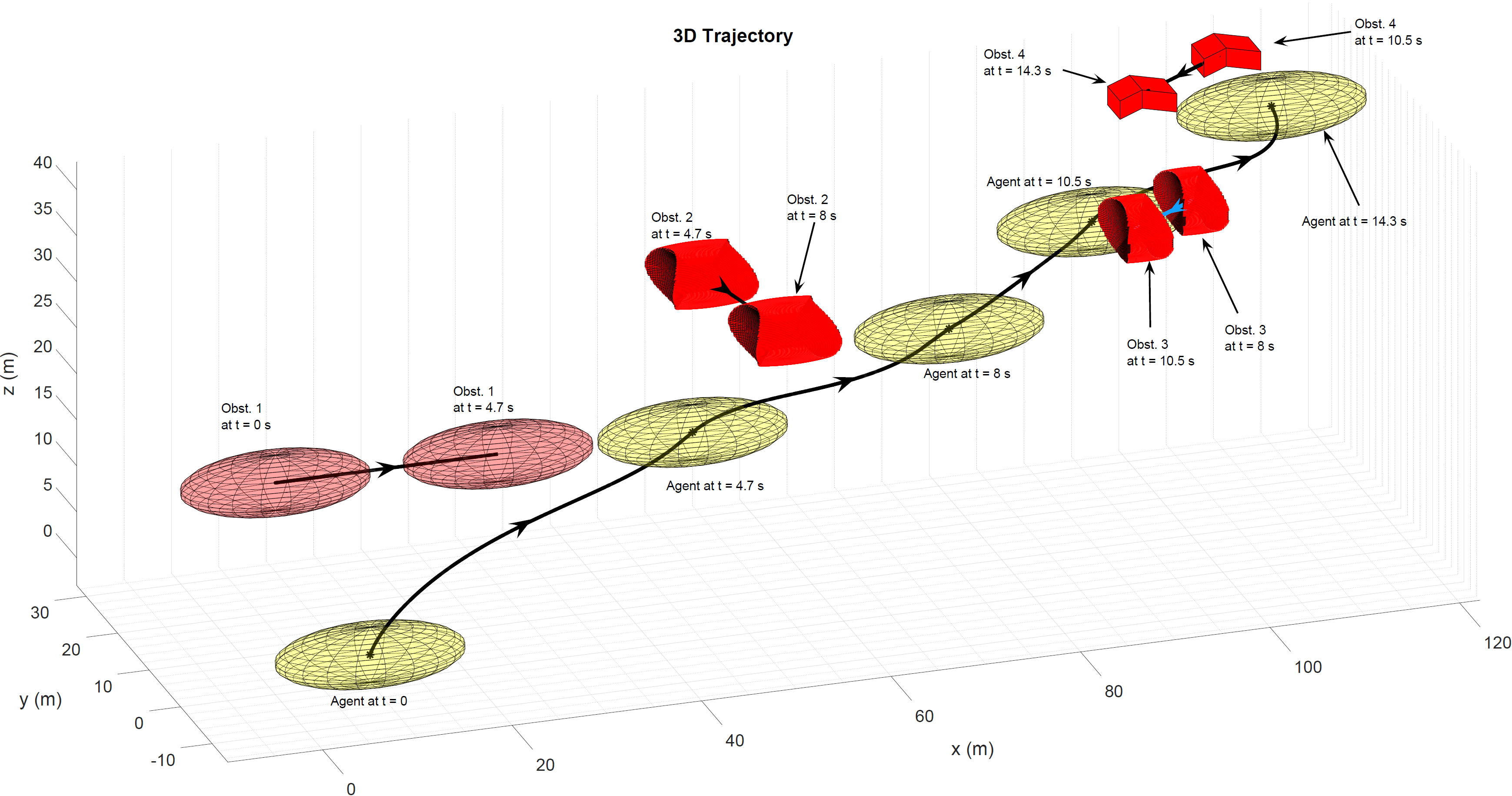
Figure 9: Simulation 1: 3D Trajectory

VI Simulation Results

Two simulation cases for a non-cooperative and cooperative collision avoidance scenario, respectively, are presented. In the non-cooperative case, an engagement geometry is chosen where the agent $A$ is an ellipsoid with center at $(10,0,0)$ at initial time $t=0$ and semi-principal axes of $10\,m,\,5\,m,\,3\,m$. Its speed is $8.5\,\,\mathrm{m/s}$ with the initial heading direction at an azimuth of $0^{\circ}$ and elevation of $69^{\circ}$, as seen in Fig 13. $A$ faces a series of four obstacles $B,C,D$ and $E$ in quick succession. $B$ is an ellipsoid with it’s center initially located at $(0,0,20)$ and having the same principal axes as $A$. Its speed is $5\,\,\mathrm{m/s}$ with an initial heading angle at an azimuth and elevation of $0^{\circ}$. For this engagement, the collision cone $y_{p}$ is computed on multiple planes using the algorithms of Section IV as shown in Fig. 10. It can be clearly seen that the value of $y_{p}$ obtained from those planes is negative at $t=0$. Since $V_{r}$ is also negative at $t=0$ (See Fig 11), both ellipsoids are on a collision course. In order to avoid $B$, the plane with the maximum value of $\psi_{p}$ (at each instant) is selected as the avoidance plane. The collision cone $y_{p}$ along with the projected value of the states is used to generate the acceleration command using (15) and the time history of the magnitude and direction of this acceleration is given Fig 12. Fig. 14 shows the time history of $y_{p}$ computed on the plane of maximum $\psi_{p}$. From this, and the plot of $V_{r}$ in Fig 11, it can be seen that both parameters become greater than zero after a certain time, signifying a successful collision avoidance maneuver. $A$ is able to fully steer away from $B$ after $4.7\,\mathrm{s}$. The next obstacle $C$ is a biconcave ellipsoid with center at $(50,15,30)$ at time $t=4.7\,\mathrm{s}$. It’s speed is $5.1\,\mathrm{m/s}$ with heading angle at an azimuth of $0^{\circ}$ and elevation of $34.5^{\circ}$. Again from the $y_{p}$ plot in Fig 10, it can be seen that at $t=4.7\,\mathrm{s}$, $A$ is on a collision course with $C$. The collision cone $y_{p}$ and value of $\psi_{p}$ on various planes is obtained using the steps described in Section IV-C. The avoidance acceleration is again computed on the plane of maximum $\psi_{p}$ and it can be seen that the heading direction vector is steered out of the cone. At $t=8\,\mathrm{s}$, $A$ encounters the next obstacle $D$ which is a shape-changing biconcave ellipsoid, whose shape transitions from an ellipsoid to a biconcave ellipsoid with varying levels of concavity. It’s center is at $(95,-5,40)$ and speed is $3.61\,\mathrm{m/s}$ with heading direction at an azimuth of $5^{\circ}$ and an elevation of $28^{\circ}$. Similar to the first two cases, avoidance acceleration is computed on the plane of maximum $\psi_{p}$ to steer the velocity vector of $A$ out of the collision cone. After $10.5\,\mathrm{s}$, the agent encounters the fourth obstacle $E$ which is a $10$ faced polyhedron with center at $(110,30,40)$ and having the speed and direction as $C$. Collision cone $y_{p}$ and $\psi_{p}$ on the various planes is obtained using the steps outlined in Section  IV-D. Acceleration is applied to avoid the obstacle and the obstacle is successfully cleared. The trajectories of the agent $A$ and all the obstacles can be viewed in Fig 9.

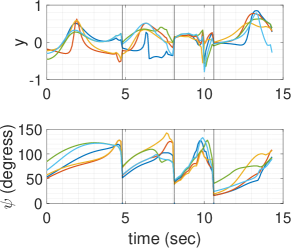
Figure 10: Simulation 1: Collision cone $y$ and $\psi$ on multiple planes

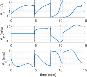
Figure 11: Simulation 1: Time histories of $V_{r}$, $V_{\theta}$ and $V_{\phi}$

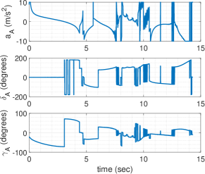
Figure 12: Time histories of acceleration and it’s direction

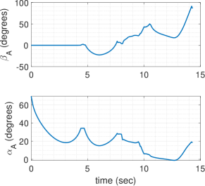
Figure 13: Simulation 1: Time histories of azimuth and elevation of heading

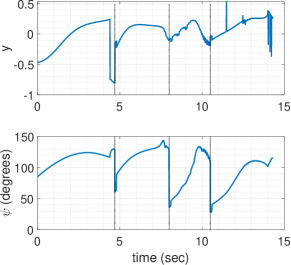
Figure 14: Simulation 1: Time histories of $y$ and $\psi$ on maximum $\psi$ plane

In the Cooperative Collision Avoidance case, $A$ is an ellipsoid, and encounters two other agents $B_{1}$ (an ellipsoid) and $B_{2}$ (a biconcave ellipsoid) in quick succession. Both pairs of agents apply avoidance accelerations cooperatively using (17). Due to page constraints, the plots for this case are not given in the paper, but are shown in the accompanying video.

VII CONCLUSIONS

In this paper, we model 3-dimensional objects having elongated and/or non-convex shapes, by using an appropriate combination of ellipsoids and one-sheeted or two-sheeted hyperboloids. The use of ellipsoids and hyperboloids provides a much tighter and less-conservative approximation to the shapes of such objects. This increases the amount of free space available for the robot trajectories. We demonstrate the construction of 3-D collision cones for such objects and present collision avoidance laws, for both cooperative as well as non-cooperative collision avoidance. Simulation results are presented.

References

- [1] C. Goerzen, Z. Kong, and B. Mettler, “A survey of motion planning algorithms from the perspective of autonomous uav guidance,” Journal of Intelligent and Robotic Systems, vol. 57, no. 1, pp. 65–100, 2010.
- [2] H. Kumar, S. Paternain, and A. Ribeiro, “Navigation of a quadratic potential with ellipsoidal obstacles,” in 2019 IEEE 58th Conference on Decision and Control (CDC), pp. 4777–4784.
- [3] Y.-K. Choi, J.-W. Chang, W. Wang, M.-S. Kim, and G. Elber, “Continuous collision detection for ellipsoids,” IEEE Transactions on visualization and Computer Graphics, vol. 15, no. 2, pp. 311–325, 2008.
- [4] H. Kumar, S. Paternain, and A. Ribeiro, “Navigation of a quadratic potential with star obstacles,” in 2020 American Control Conference (ACC), pp. 2043–2048.
- [5] A. Chakravarthy and D. Ghose, “Obstacle avoidance in a dynamic environment: A collision cone approach,” IEEE Transactions on Systems, Man, and Cybernetics-Part A: Systems and Humans, vol. 28, no. 5, pp. 562–574, 1998.
- [6] P. Fiorini and Z. Shiller, “Motion planning in dynamic environments using velocity obstacles,” The International Journal of Robotics Research, vol. 17, no. 7, pp. 760–772, 1998.
- [7] J. Van Den Berg, D. Wilkie, S. J. Guy, M. Niethammer, and D. Manocha, “Lqg-obstacles: Feedback control with collision avoidance for mobile robots with motion and sensing uncertainty,” in 2012 IEEE International Conference on Robotics and Automation.
- [8] A. Chakravarthy and D. Ghose, “Collision cones for quadric surfaces,” IEEE Transactions on Robotics, vol. 27, no. 6, pp. 1159–1166, 2011.
- [9] ——, “Generalization of the collision cone approach for motion safety in 3-d environments,” Autonomous Robots, vol. 32, no. 3, 2012.
- [10] A. Ferrara and C. Vecchio, “Second order sliding mode control of vehicles with distributed collision avoidance capabilities,” Mechatronics, vol. 19, no. 4, pp. 471–477, 2009.
- [11] Y. Watanabe, A. Calise, E. Johnson, and J. Evers, “Minimum-effort guidance for vision-based collision avoidance,” in AIAA atmospheric flight mechanics conference and exhibit, 2006, p. 6641.
- [12] P. Karmokar, K. Dhal, W. J. Beksi, and A. Chakravarthy, “Vision-based guidance for tracking dynamic objects,” in 2021 International Conference on Unmanned Aircraft Systems (ICUAS), pp. 1106–1115.
- [13] E. Lalish and K. A. Morgansen, “Distributed reactive collision avoidance,” Autonomous Robots, vol. 32, no. 3, pp. 207–226, 2012.
- [14] B. L. Boardman, T. L. Hedrick, D. H. Theriault, N. W. Fuller, M. Betke, and K. A. Morgansen, “Collision avoidance in biological systems using collision cones,” in 2013 American Control Conference. IEEE, 2013, pp. 2964–2971.
- [15] W. Zuo, K. Dhal, A. Keow, A. Chakravarthy, and Z. Chen, “Model-based control of a robotic fish to enable 3d maneuvering through a moving orifice,” IEEE Robotics and Automation Letters, vol. 5, no. 3, pp. 4719–4726, 2020.
- [16] K. Dhal, A. Kashyap, and A. Chakravarthy, “Collision avoidance and rendezvous of quadric surfaces moving in planar environments,” in To be presented in the proceedings of 2021 IEEE Control and Decision Conference. IEEE, 2021.
- [17] K. Tholen, V. Sunkara, A. Chakravarthy, and D. Ghose, “Achieving overlap of multiple, arbitrarily shaped footprints using rendezvous cones,” Journal of Guidance, Control, and Dynamics, vol. 41, no. 6, pp. 1290–1307, 2018.
- [18] K. S. Arun, T. S. Huang, and S. D. Blostein, “Least-squares fitting of two 3-d point sets,” IEEE Transactions on Pattern Analysis and Machine Intelligence, vol. PAMI-9, no. 5, pp. 698–700, 1987.