An Active Contour Model with Local Variance Force Term and Its Efficient Minimization Solver for Multi-phase Image Segmentation

Abstract

In this paper, we propose an active contour model with a local variance force (LVF) term that can be applied to multi-phase image segmentation problems. With the LVF, the proposed model is very effective in the segmentation of images with noise. To solve this model efficiently, we represent the regularization term by characteristic functions and then design a minimization algorithm based on a modification of the iterative convolution-thresholding method (ICTM), namely ICTM-LVF. This minimization algorithm enjoys the energy-decaying property under some conditions and has highly efficient performance in the segmentation. To overcome the initialization issue of active contour models, we generalize the inhomogeneous graph Laplacian initialization method (IGLIM) to the multi-phase case and then apply it to give the initial contour of the ICTM-LVF solver. Numerical experiments are conducted on synthetic images and real images to demonstrate the capability of our initialization method, and the effectiveness of the local variance force for noise robustness in the multi-phase image segmentation.

68U10, 65K10, 65M12, 62H35, 94A08

1 Introduction

Image segmentation is a process of partitioning an image into disjoint segments according to the certain characterization of the contents in the image. It plays a fundamental role in the visual information analysis processes, including object detection, image recognition, and visual field monitoring [1, 24, 28].

Various approaches have been proposed for image segmentation problems over the last few decades, among which active contour models are widely used in many fields and enjoy great success [9, 12, 13, 15, 22, 25]. The basic procedure for active contour models achieving image segmentation is first creating an initial contour or region and then driving it to evolve to the object edges or covering the object according to edge-based or region-based information from the image. In the edge-based active contour models, the evolution of the contour is mainly dependent on the gradient information, which makes it sensitive to the initialization, noise, and intensity strength of the boundary [16, 23]. Region-based active contour models [2, 12, 17, 18, 25, 31, 35, 40, 41] typically define an energy functional over the image domain and all segments. Minimizing these well-designed energy functionals, one can obtain desired segmentation results. Compared to the edge-based active contour models, region-based ones have better performance on images with noise and weak boundaries.

Besides the models, the minimization methods of the energy functionals are also of great importance for image segmentation. In the region-based active contour models, the alternative direction method can effectively simplify the process of the minimization for multi-variable energy functionals [14, 37, 38]. Then the gradient descent method is commonly used to locate the contours’ positions where the energy functional reach its minimum, see for instance, the celebrated level set method introduced by Osher and Sethian in [26], where the choice of the numerical method plays an important role for solving the derived partial differential equation. An improper numerical method will result in inefficiency, even instability. Recently, Wang et al. [33, 34] proposed a new framework for the minimization of the energy functional in the region-based active contour models in which segments are represented by their characteristic functions, and a concave functional is used to approximate the contour length. Then an ICTM is proposed in this framework to minimize the modified energy functionals in an efficient and energy stable way. This framework is applicable to a wide range of active contour models and can be implemented in a simple and efficient way for both binary and multi-phase segmentation. But for images with noise, the segmentation results of ICTM will not be so satisfying when it is applied to some noise-sensitive active contour models.

In addition to the challenge by the noise, region-based active contour models are also facing an initialization issue. The initial contour significantly affects segmentation results since most of the energy functionals in the region-based active contour models are non-convex. A feasible solution for this initialization issue is to relax the energy functional into a convex functional [3, 4, 5, 6, 8, 11, 29, 36]. However, convex relaxation deprives all the non-convex parts of the original energy functional, and hence may entail the loss of non-convex information of the segments and reduce models’ capability of preserving the sharpness and neatness of edges [10, 39]. Very recently, Qiao and Zhang proposed an initialization method [30] where the non-local Laplacian operator is employed to select the initial contour. Compared to the typical choice, for instance, select artificially, or through some simple threshold, [14, 19, 34, 40], the detected initial contour can reduce the sensitivity of initialization. But for images with intensity inhomogeneity, it may not work. To handle this problem, Liu et al. [20] developed an IGLIM for binary segmentation, which can give reliable initial contours on grayscale images even with intensity inhomogeneity. For the multi-phase segmentation problem, the selection for the initial contour will become more tricky and sensitive, and an improper initialization will cause an unacceptable segmentation result.

In this paper, we propose a new region-based active contour model with a local variance force term. Similar to the model in [34], segments are represented by their characteristic functions, and a concave functional is used to approximate the contour length. The local variance force term can help to segment images with noise in a highly effective way. Then we develop an ICTM-LVF solver to minimize the proposed energy to achieve highly efficient segmentation. To get reliable initial contours for the minimization solver, we generalize the IGLIM to the multi-phase case and propose the Multi-IGLIM. The rest of this paper is organized as follows. In Section 2, we introduce the LVF and propose the new active contour model. In Section 3, we design the ICTM-LVF algorithm for solving the developed model with the initialization by the Multi-IGLIM. The energy dissipation of the ICTM-LVF is also proved in this section. Numerical experiments are given in Section 4 to show the effectiveness of the Multi-IGLIM and the performance of the ICTM-LVF solver. Comparisons are also made between the ICTM-LVF solver and some state-of-art image segmentation methods. Finally, the paper ends with some conclusions in Section 5.

2 Proposed model

In this section, we will propose a new active contour model with a local variance force term. First, we will briefly review some region-based active contour models and present the general form of their energy functionals. Then a local variance force is introduced to improve the robustness to noise of active contour models.

2.1 General energy functionals for region-based active contour models

Region-based active contour models achieve image segmentation by minimizing energy functionals that are defined on segments. To make it more clear, we will provide two representative models. The first one is the Chan-Vese (CV) model [12, 32] in which the energy functional for an $n$-phase image can be defined as follows:

(1) $$E_{CV}(\Omega_{1},\cdots,\Omega_{n},c_{1},\cdots,c_{n})=\sum_{i=1}^{n}\int_{\Omega_{i}}\lambda_{i}|I(x)-c_{i}|^{2}dx+\mu\sum_{i=1}^{n}|\partial\Omega_{i}|,$$

where $\Omega_{i}$ represents the $i$-th segment whose boundary is $\partial\Omega_{i}$, $|\partial\Omega_{i}|$ denotes the length of $\partial\Omega_{i}$, $\lambda_{i}$, $\mu$ are fixed positive parameters, and $c_{i}$ is a constant used to approximate the average of the image intensity $I$ within $\Omega_{i}$. Once the image $I$ is given, our goal is to find suitable partitions with $\Omega_{i}$ and $c_{i}$ such that $E_{CV}$ reaches its minimum. The CV model is a classic and effective region-based active contour model. However, the CV model assumes that the intensity is constant on all segments, which makes it inappropriate for images with intensity inhomogeneity. To tackle the segmentation difficulty caused by intensity inhomogeneity, another widely used model, the local binary fitting (LBF) model, was given in [17, 18]. This model was originally proposed for two-phase image segmentations. But generally, the local image fitting (LIF) model can achieve an $n$-phase segmentation, whose energy functional is defined as

(2) $$E_{LIF}(\Omega_{1},\cdots,\Omega_{n},f_{1},\cdots,f_{n})=\sum_{i=1}^{n}\lambda_{i}\int_{\Omega}\int_{\Omega_{i}}G_{\sigma}(x-y)|I(y)-f_{i}(x)|^{2}dydx+\mu\sum_{i=1}^{n}|\partial\Omega_{i}|,$$

where

(3) $$G_{\sigma}(x)=\frac{1}{2\pi\sigma}e^{-\frac{|x|^{2}}{2\sigma}}$$

is a two-dimensional Gaussian kernel with standard deviation $\sigma$, and $f_{i}(x)$ are local intensity fitting functions.

The CV model and the LIF model are two representative region-based active contour models whose energy functionals consist of a fidelity term and a regularized term $\mu\sum_{i=1}^{n}|\partial\Omega_{i}|$. In fact, as shown in [34], numerous active contour models are similar in terms of the form of the energy functional (a fidelity term and a regularized term). From these models, one can abstract a rather general energy functional:

(4) $$\begin{split}E_{g}(u_{1},\cdots,u_{n},\Theta_{1},\cdots,\Theta_{n})&=\sum_{i=1}^{n}\lambda_{i}\int_{\Omega}u_{i}F_{i}(I,\Theta_{1},\cdots,\Theta_{n})dx\\ &\quad+\mu\sum_{i=1}^{n}\sum\limits_{j=1,j\neq i}^{n}\sqrt{\frac{\pi}{\tau}}\int_{\Omega}u_{i}G_{\tau}*u_{j}dx,\end{split}$$

where $\Theta_{i}=(\Theta_{i,1},\cdots,\Theta_{i,n})$ denotes all possible variables or functions in the fidelity term. In the model of (4), all the segments are represented by their characteristic functions $u=(u_{1},u_{2},\cdots,u_{n})$ and $|\partial\Omega_{i}|$ is approximated by

$$\sum\limits_{j=1,j\neq i}^{n}\sqrt{\frac{\pi}{\tau}}\int_{\Omega}u_{i}G_{\tau}*u_{j}dx,$$

where $\tau$ is the standard derivation of the Gaussian kernel $G_{\tau}$ and $*$ denotes the convolution.

To minimize the energy functional Eq. 4 for image segmentation, Wang et al. [34] proposed an efficient numerical solver, called the ICTM, which has energy-decaying property and can converge rapidly in numerical experiments. Despite efforts of the ICTM to increase the convergence speed and stability in the segmentation, initialization and noise robustness are still two significant issues for active contour models. In this paper, we will develop a new region-based active contour model with a local variance force term, which has better performance in the segmentation of images with noise and can be solved by a majority minimization method that is similar to the ICTM. Our minimization algorithm also enjoys the energy-decaying property under some conditions and can converge rapidly in experiments on various images.

2.2 Local variance force

In this part, we introduce a local variance force which can be combined with the original energy (4) to ameliorate segments’ robustness to noise and lead to a smooth segmentation result for images with noise.

The local variance force for $x\in\Omega$ in the $i$-th phase is defined as follows:

(5) $$F_{i}^{LV}(I,m_{i})=\sum\limits_{y\in K_{r}(x)}|I(y)-m_{i}|^{2},$$

where $I$ is a given image, $r$ is a given positive integer, $K_{r}(x)$ is a square of $(2r+1)\times(2r+1)$ pixels centered at $x$, and $m_{i}$ is an approximated mean intensity of the non-degenerated images in the $i$-th phase.

For degenerated images, such as images with noise or intensity inhomogeneity, it is not easy to find the exact mean value of pixel intensities of the non-degenerated images in a small local region. However, the intensity value can be approximated by some constants or functions, which is a commonly approach in active contour models. For instance, the CV model uses the mean values of the segments to approximate the non-degenerated intensity value of each pixel in different phases:

$$m_{i}\approx c_{i}=\frac{\int_{\Omega}u_{i}Idx}{\int_{\Omega}u_{i}dx}.$$

In the LBF/LIF model, the following functions are used to approximate the local mean image intensities for each pixel in different phases:

$$m_{i}\approx f_{i}=\frac{\int_{\Omega}u_{i}(y)G_{\sigma}(y-x)I(y)dy}{\int_{\Omega}u_{i}(y)G_{\sigma}(y-x)dy}.$$

Typically, $m_{i}$ is related to $I$, and $u_{i}$, therefore we can approximate $m_{i}$ by some prior estimating functionals which we denote by $M(I,u_{i})$.

For the CV model, the prior mean intensity estimating functional can be chosen as:

$$M(I,u_{i})=\frac{\int_{\Omega}u_{i}Idx}{\int_{\Omega}u_{i}dx}.$$

For the LBF/LIF model, we have two choices:

$$M(I,u_{i})=\frac{\int_{\Omega}u_{i}Idx}{\int_{\Omega}u_{i}dx}\quad\text{ or }\quad M(I,u_{i})=\frac{\int_{\Omega}u_{i}(y)G_{\sigma}(y-x)I(y)dy}{\int_{\Omega}u_{i}(y)G_{\sigma}(y-x)dy}.$$

2.3 New active contour model with a local variance force term

Since the variance of local regions should be relatively small in a proper segmentation, we can use Eq. 5 to evaluate the fitness of $x\in\Omega$ in the $i$-th phase. In fact, for most of noise-sensitive models, the local variance is not considered. As a result, pixels with noise are prone to be divided into an improper segment. In view of this, we add the local variance force to the original energy Eq. 4 to prevent the misclassification caused by the noise and ensure the smoothness of the segmentation result. The modified energy is given below.

(6) $$E(u,\Theta,m) =\sum_{i=1}^{n}\lambda_{i}\int_{\Omega}u_{i}F_{i}(I,\Theta_{1},\cdots,\Theta_{n})dx+\mu\sum_{i=1}^{n}\sum\limits_{j=1,j\neq i}^{n}\sqrt{\frac{\pi}{\tau}}\int_{\Omega}u_{i}G_{\tau}*u_{j}dx,$$

$$+p\sum_{i=1}^{n}\lambda_{i}\int_{\Omega}\int_{\Omega}u_{i}(x)K_{r}(y-x)(I(y)-m_{i}(x))^{2}dydx,$$

where $p$ is a positive constant.

3 Numerical method

In this part, we develop an efficient numerical solver, the ICTM-LVF minimization algorithm, to solve the proposed energy model (6) for the multi-phase segmentation. To get a proper initial contour for the minimization process, we employ the Multi-IGLIM, which is generalized from the IGLIM proposed in [20].

3.1 Multi-IGLIM

The IGLIM is merely designed for binary segmentation. We can generalize it to the multi-phase case through K-means to give initial contours of active contour models for multi-phase segmentation.

The IGLIM generates initial contours according to the information derived from an anisotropic Laplacian operator, namely the inhomogeneous graph Laplacian operator. Moreover, a denoising step is performed in the IGLIM to remove the possible noise effect and obtain more reliable initial contours.

3.1.1 Inhomogeneous graph Laplacian operator

Let $\Omega$ be a 2D discrete image domain, and $I$ be an image defined on it with $M_{1}\times M_{2}$ pixels. Denote a pixel $x_{0}=(i,j)\in\Omega$, its corresponding intensity vector $I(x_{0})$ by $I_{i,j}$. The inhomogeneous graph Laplacian operator $L$ is defined as

(7) $$L(x_{0})=\sum_{k=1}^{8}\sum_{p=1}^{r}c_{k}I_{i,j}^{k}(p)-I_{i,j}(p),$$

where $r$ is the number of channels, and $I_{i,j}^{k}$ is the intensity vector of the $k$-th neighbour point of $I_{i,j}$, more precisely,

$$I_{i,j}^{1}=I_{i-1,j-1},I_{i,j}^{2}=I_{i-1,j},I_{i,j}^{3}=I_{i-1,j+1},I_{i,j}^{4}=I_{i,j+1},$$

$$I_{i,j}^{5}=I_{i+1,j+1},I_{i,j}^{6}=I_{i+1,j},I_{i,j}^{7}=I_{i+1,j-1},I_{i,j}^{8}=I_{i,j-1},$$

and

$$c_{k}=\frac{\sum_{p=1}^{r}e^{\lambda(I_{i,j}(p)-I_{i,j}^{k}(p))^{2}}}{\sum_{k=1}^{8}\sum_{p=1}^{r}e^{\lambda(I_{i,j}(p)-I_{i,j}^{k}(p))^{2}}},\text{ $\lambda$ is a given non-negative parameter}.$$

The parameter $r$ equals 1 when the target image is grayscale, while $r$ of a color image is usually set to 3 corresponding to the R, G, B channel, respectively. We then approximate the zero-cross points of the inhomogeneous Laplacian operator to obtain rough initial edges. The edge points are divided into two groups $S_{p}$ and $S_{n}$ according to the sign of the inhomogeneous Laplacian value. The readers may refer to [20] for a more detailed description of the inhomogeneous graph Laplacian operator.

3.1.2 A denoising method based on the connectivity of edge points

The research in [20] gives a denoising method based on the diagonal connectivity of edge points to remove some possible noise pixels from the rough initial contour obtained from the inhomogeneous graph Laplacian operator. The diagonally connected points are defined as follows:

Definition 3.1.

[20] When $x=(i,j)\in S_{p}$ ($S_{n}$), the neighbor areas are divided into four parts:

$$S_{1}=\{(i-1,j-1),(i,j-1),(i-1,j)\},\ S_{2}=\{(i-1,j+1),(i,j+1),(i-1,j)\},$$

$$S_{3}=\{(i+1,j-1),(i,j-1),(i+1,j)\},\ S_{4}=\{(i+1,j+1),(i,j+1),(i+1,j)\}.$$

We call $x\in S_{p}$ ($S_{n}$) a diagonally connected point if both $S_{1}$ and $S_{4}$ or both $S_{2}$ and $S_{3}$ have at least one pixel that also belongs to $S_{p}$ ($S_{n}$).

To eliminate the noise in the rough initial contour, the IGLIM keeps all the diagonally connected points in $S_{p}$ ($S_{n}$) and removes the other points from $S_{p}$ ($S_{n}$). The denoising process needs to be repeated $M$ times where $M$ is a pre-setting small integer.

For a better understanding of the Multi-IGLIM, we display the algorithm for the IGLIM in Algorithm 1.

Algorithm 1 IGLIM [20]

0:  $I,\lambda,\alpha,M$

0:  Initial contours for binary phases $u^{0}$

1:  Compute the inhomogeneous Laplacian value of each pixel by (7).

2:  Set a small positive number $\alpha$. Determine $S_{p}$ and $S_{n}$ according to the sign of the inhomogeneous Laplacian value at each pixel.

3:  Take $S_{p}$ $(S_{n})$ as a rough initial contour.

4:  Go through every pixel in $S_{p}$ $(S_{n})$ and judge whether it is diagonally connected. If not, remove it from $S_{p}$ $(S_{n})$.

5:  Set an appropriate integer $M$, and repeat Step 4 for $M$ times.

6:  Output $S_{p}$ $(S_{n})$ as the initial contour $u^{0}$.

3.1.3 Algorithm for the Multi-IGLIM

Since there are only two cases for the sign of inhomogeneous graph Laplacian operator, i.e., positive and negative, the IGLIM can only be applied to binary image segmentation. For the multi-phase image segmentation, we generalize the IGLIM to the Multi-IGLIM for the initialization. First, we determine all the possible edge points through their absolute values of inhomogeneous graph Laplacian rather than from their signs. If the absolute value is larger than a certain threshold, its corresponding point will be regarded as a possible edge point. Then when all the possible edge points are located, we employ K-means to divide all the edge points into different phases according to their pixel values. The algorithm of the Multi-IGLIM is summarized in Algorithm 2.

Algorithm 2 Multi-IGLIM

0:  $I,\lambda,\alpha,M,n$

0:  Initial contours for $n$ phases $u^{0}=(u_{1}^{0},u_{2}^{0},\cdots,u_{n}^{0})$

1:  Compute the inhomogeneous graph Laplacian value of each pixel by (7).

2:  Set a small positive number $\alpha$. Put all together pixels $x$ whose $|L(x)|\geq\alpha$ into a set denoted as $S$.

3:  Divide into $n$ separate sets all pixels of $S$ by K-means according to their pixel values. Denote these sets as $S_{1},\cdots,S_{n}$.

4:  Go through every pixel in $S_{1},\cdots,S_{n}$ and judge whether it is diagonally connected in their set. If not, remove it from their set.

5:  Set an appropriate integer $M$, and repeat Step 4 for $M$ times.

6:  Output the characteristic function of $S_{i},i=1,\cdots,n$, which is defined as $u_{i}^{0}$, as the initial contours.

3.2 ICTM-LVF solver

To solve the proposed model Eq. 6 efficiently, we develop a minimization algorithm, viz. the ICTM-LVF solver.

Similar to the ICTM [34], we split the original problem into two optimization problems instead of solving it directly. Given an initial segments $u^{0}=(u_{1}^{0},u_{2}^{0},\cdots,u_{n}^{0})$ obtained from the Multi-IGLIM in Algorithm 2, we can update $\Theta,m$ and $u$ as follows:

(8) $$\left\{\begin{array}[]{ll}\displaystyle\Theta^{k}=\arg\min_{\Theta}E(u^{k},\Theta),\\ \displaystyle m^{k}=M(I,u^{k}),\\ \displaystyle u^{k+1}=\arg\min_{u\in\mathcal{S}}E(u,\Theta^{k},m^{k}),\end{array}\right.$$

for $k=0,1,2,\cdots$, where $\mathcal{S}:=\{(u_{1},u_{2},\cdots,u_{n})|u_{i}\in[0,1],\sum_{i=1}^{n}u_{i}=1\}.$

Note that

$$E(u,\Theta^{k},m^{k})=E(u^{k},\Theta^{k},m^{k})+L(u,u^{k},\Theta^{k},m^{k})+h.o.t.$$

Here

(9) $$L(u,u^{k},\Theta^{k},m^{k})=\sum_{i=1}^{n}\int_{\Omega}u_{i}\phi_{i}^{k}dx=\int_{\Omega}\sum_{i=1}^{n}\phi_{i}^{k}u_{i}dx,$$

where

$$\phi_{i}^{k}=\lambda_{i}F_{i}(I,\Theta^{k})+2\mu\sqrt{\frac{\pi}{\tau}}\sum\limits_{j=1,j\neq i}^{n}G_{\tau}*u_{j}^{k}+p\lambda_{i}K_{r}*(I-m_{i}^{k})^{2}.$$

Instead of solving $u^{k+1}=\arg\min_{u}E(u,\Theta^{k},m^{k})$ in (8), we approximate $u^{k+1}$ by minimizing the linearized functional Eq. 9 of $E(u,\Theta^{k},m^{k})$ as

(10) $$u^{k+1}=\arg\min_{u}L(u,u^{k},\Theta^{k},m^{k}).$$

From Eq. 9, one can compare the coefficients $\phi_{i}^{k}(x)$ of $u_{i}$ for a fixed point $x$ and find that the minimum for $L$ with respect to $u$ is attained at

$$u_{i}(x)=\begin{cases}1\quad\text{if }i=\arg\min_{l\in[n]}\phi_{l}^{k},\\ 0\quad\text{otherwise}.\end{cases}$$

Therefore, solving Eq. 10 for $u^{k+1}$ can be carried out at each $x\in\Omega$ independently. The algorithm of ICTM-LVF is displayed in Algorithm 3. Compared with the original ICTM, a local variance force based on a prior mean estimating function is introduced when updating $u$. In fact, in the original ICTM, the update procedure of $u$ is also independently carried out at each $x\in\Omega$, which makes it outperform the classical level set method in terms of efficiency. However, the ICTM suffers from the noise heavily since the value of $u_{i}^{k+1}$ merely depends on the intensity of a single pixel. While in the ICTM-LVF algorithm, an index of the fitness of segments, i.e., the local variance force, is considered at each $x\in\Omega$ when $u$ is updated. As we can see from the numerical experiments in Section 4, the local variance force term can effectively reduce the noise effect. In addition, the energy-decaying property for the ICTM-LVF solver can also be guaranteed under some conditions.

Algorithm 3 ICTM-LVF

0:  $I,u^{0}$

0:  Segmentation Results $u^{s}$

1:  Set $k=0$

2:  while not converged do

3:     For the fixed $u^{k}$, find

$$\Theta^{k}=\arg\min\limits_{\Theta}\sum_{i=1}^{n}\lambda_{i}\int_{\Omega_{i}}u_{i}F_{i}(I,\Theta)dx.$$

4:     For the fixed $u^{k}$, update

$$m^{k}=M(I,u^{k}).$$

5:     For $i\in[n]$, evaluate

$$\phi_{i}^{k}=F_{i}(I,\Theta^{k})+pF_{i}^{LV}(I,m^{k})+2\mu\sum\limits_{j=1,j\neq i}^{n}\sqrt{\frac{\pi}{\tau}}G_{\tau}*u_{j}^{k}.$$

6:     For $i\in[n]$, set

$$u_{i}^{k+1}=\begin{cases}1\quad\text{if }i=\min\{\arg\min_{l\in[n]}\phi_{l}^{k}\},\\ 0\quad\text{otherwise}.\end{cases}$$

7:  end while

8:   Set $k=k+1$

3.3 Energy-decaying property for the ICTM-LVF

In this part, we will prove the energy-decaying property for the ICTM-LVF under some conditions. Firstly, we will introduce two lemmas related to the discrete convolution.

Lemma 3.2.

Given $u(x):\mathbb{R}\to\mathbb{R}$, let $g(x)=\frac{1}{\sqrt{2\pi\sigma}}e^{-\frac{x^{2}}{2\sigma}},g_{k}=g(k),u_{k}=u(k)$, and

$$U=\left[u_{0},u_{1},\cdots,u_{n-1}\right]^{T}.$$

Define the discrete form of the convolution $g*u$ on the meshgrid $[0,1,2,\cdots,n-1]$ by an $n\times 1$ vector $D_{g*u}$ as follows:

$$D_{g*u}(k)=\sum_{i=-\lceil\frac{n}{2}-1\rceil}^{\lfloor\frac{n}{2}\rfloor}g(-i)u(k-1+i),\quad k=1,\cdots,n.$$

Then $D_{g*u}$ can be expressed as the product of a matrix $G$ and $U$ if $u$ is under the periodic boundary condition. Moreover, if $\sigma<\frac{1}{2}$, $G$ is positive definite and all its eigenvalues are larger than a positive constant independent on $n$.

Proof 3.3.

Let

$$G=\left[\begin{array}[]{cccccccc}g_{0}&g_{1}&\ldots&g_{\lfloor\frac{n}{2}\rfloor}&g_{\lceil\frac{n}{2}-1\rceil}&\ldots&g_{2}&g_{1}\\ g_{1}&g_{0}&g_{1}&\ldots&g_{\lfloor\frac{n}{2}\rfloor}&\ddots&g_{3}&g_{2}\\ \vdots&\ddots&\ddots&\ddots&\ldots&\ddots&\ddots&\vdots\\ g_{\lfloor\frac{n}{2}\rfloor}&\ddots&\ddots&\ddots&\ddots&\ldots&\ddots&\ddots\\ g_{\lceil\frac{n}{2}-1\rceil}&\ddots&\ddots&\ddots&\ddots&\ddots&\ldots&\ddots\\ \vdots&\ddots&\ddots&\ddots&\ddots&\ddots&\ddots&\ldots\\ g_{2}&\ldots&g_{\lceil\frac{n}{2}-1\rceil}&g_{\lfloor\frac{n}{2}\rfloor}&\ldots&g_{1}&g_{0}&g_{1}\\ g_{1}&g_{2}&\ldots&g_{\lceil\frac{n}{2}-1\rceil}&g_{\lfloor\frac{n}{2}\rfloor}&\ldots&g_{1}&g_{0}\end{array}\right].$$

Then we have

$$\left[GU\right]_{k} =\sum_{i=-\lceil\frac{n}{2}-1\rceil}^{\lfloor\frac{n}{2}\rfloor}g(i)u(k-1+i)$$

$$=\sum_{i=-\lceil\frac{n}{2}-1\rceil}^{\lfloor\frac{n}{2}\rfloor}g(-i)u(k-1+i),$$

$$=D_{g*u}(k),$$

where $k=1,\cdots,n,$ and $\left[GU\right]_{k}$ represents the $k$th entry of $GU$. Therefore,

$$D_{g*u}=GU.$$

Note that $G$ is a circulant matrix, we can obtain its eigenvalues by calculating the product of discrete Fourier transform matrix $F$ and the first column of $G$, and then we can find they are all not less than a certain positive constant. Indeed, denoting by $v$ the first column of $G$, we have

$$\left[Fv\right]_{j} =\frac{1}{\sqrt{2\pi\sigma}}\sum_{k=1}^{n}e^{\frac{2(k-1)j\pi i}{n}}G_{k,1}$$

$$\geq\frac{1}{\sqrt{\pi}}(1-\sum_{k=1}^{\lfloor\frac{n}{2}\rfloor}2e^{-k^{2}})$$

$$\geq\frac{1}{\sqrt{\pi}}(1-\sum_{k=1}^{\infty}2e^{2-3k})$$

$$=\frac{1}{\sqrt{\pi}}(1-\frac{2e^{2}}{e^{3}-1})$$

$$>0,$$

where $\left[Fv\right]_{j}$ represents the $j$th entry of $Fv$.

Lemma 3.2 can be generalized to the 2D case.

Lemma 3.4.

Given $u(x,y):\mathbb{R}^{2}\to\mathbb{R}$, let $g(x)=\frac{1}{2\pi\sigma}e^{-\frac{x^{2}+y^{2}}{2\sigma}},g_{k}=\frac{1}{\sqrt{2\pi\sigma}}e^{-\frac{k^{2}}{2\sigma}},u_{k_{1},k_{2}}=u(k_{1},k_{2})$, and $U=(u_{i,j})_{m\times n}.$ Define the discrete form of the convolution $g*u$ on the meshgrid $[0,1,2,\cdots,n-1]\times[0,1,2,\cdots,n-1]$ by an $m\times n$ matrix $D_{g*u}$, where for $p=1,\cdots,m,\quad q=1,\cdots,n$,

$$D_{g*u}(p,q)=\sum_{i=-\lceil\frac{m}{2}-1\rceil}^{\lfloor\frac{m}{2}\rfloor}\sum_{j=-\lceil\frac{n}{2}-1\rceil}^{\lfloor\frac{n}{2}\rfloor}g(-i)g(-j)u(p-1+i,q-1+j).$$

Then $V(D_{g*u})$ can be expressed as the product of a matrix $G$ and $V(U)$ if $u$ is under the periodic boundary condition. Here $V$ denotes the vectorization operator and

$$V(A)=[a_{1}^{T},\cdots,a_{n}^{T}]^{T}$$

for any $m\times n$ matrix $A=\left[a_{1},\cdots,a_{n}\right]$. Moreover, if $\sigma<\frac{1}{2}$, $G$ is positive definite and all its eigenvalues are larger than a positive constant independent on $m$ or $n$.

Proof 3.5.

Let

$$G_{n}=\left[\begin{array}[]{cccccccc}g_{0}&g_{1}&\ldots&g_{\lfloor\frac{n}{2}\rfloor}&g_{\lceil\frac{n}{2}-1\rceil}&\ldots&g_{2}&g_{1}\\ g_{1}&g_{0}&g_{1}&\ldots&g_{\lfloor\frac{n}{2}\rfloor}&\ddots&g_{3}&g_{2}\\ \vdots&\ddots&\ddots&\ddots&\ldots&\ddots&\ddots&\vdots\\ g_{\lfloor\frac{n}{2}\rfloor}&\ddots&\ddots&\ddots&\ddots&\ldots&\ddots&\ddots\\ g_{\lceil\frac{n}{2}-1\rceil}&\ddots&\ddots&\ddots&\ddots&\ddots&\ldots&\ddots\\ \vdots&\ddots&\ddots&\ddots&\ddots&\ddots&\ddots&\ldots\\ g_{2}&\ldots&g_{\lceil\frac{n}{2}-1\rceil}&g_{\lfloor\frac{n}{2}\rfloor}&\ldots&g_{1}&g_{0}&g_{1}\\ g_{1}&g_{2}&\ldots&g_{\lceil\frac{n}{2}-1\rceil}&g_{\lfloor\frac{n}{2}\rfloor}&\ldots&g_{1}&g_{0}\end{array}\right].$$

Then we have

$$D_{g*u}=G_{m}UG_{n},$$

and

$$V(D_{g*u})=V(G_{m}UG_{n})=(G_{n}\otimes G_{m})V(U),$$

where $\otimes$ is the Kronecker product. Note that

$$G_{n}\otimes G_{m} =(F_{n}^{-1}\Lambda_{n}F_{n})\otimes(F_{m}^{-1}\Lambda_{m}F_{m})$$

$$=(F_{n}^{-1}\otimes F_{m}^{-1})(\Lambda_{n}\otimes\Lambda_{m})(F_{n}\otimes F_{m}).$$

According to Lemma 3.2, when $\sigma<\frac{1}{2}$, all diagonal entries of $\Lambda_{n}$ and $\Lambda_{m}$ are larger than a positive constant that is not dependent on $m$ or $n$, which implies $G_{n}\otimes G_{m}$ is also positive definite and all its eigenvalues are larger than a positive constant independent on $m$ or $n$. Hence, we can obtain the desired $G$ by letting $G=G_{n}\otimes G_{m}$.

The following theorem gives the energy-decaying property of the ICTM-LVF solver displayed in Algorithm 3.

Theorem 3.6.

Given $(u^{k},\Theta^{k})$ at the $k$-th iteration in Algorithm 3. Suppose that the mean intensity estimating functional $M(I,u)$ is Lipschitz continuous w.r.t. $u$. If $\mu$ is sufficiently large and $\tau<\frac{1}{2}$, then

(11) $$E(u^{k+1},\Theta^{k+1},m^{k+1})\leq E(u^{k},\Theta^{k},m^{k}),$$

where $E$ is defined in Eq. 6.

Proof 3.7.

Let

$$E_{1}(u,\Theta)=\sum_{i=1}^{n}\lambda_{i}\int_{\Omega}u_{i}F_{i}(I,\Theta)dx+\mu\sum_{i=1}^{n}\sum\limits_{j=1,j\neq i}^{n}\sqrt{\frac{\pi}{\tau}}\int_{\Omega}u_{i}G_{\tau}*u_{j}dx,$$

$$E_{2}(u,m)=p\sum_{i=1}^{n}\lambda_{i}\int_{\Omega}u_{i}K_{r}*(I-m_{i})^{2}dx,$$

$$L(u,m,u^{k},\Theta^{k})=\sum_{i=1}^{n}\int_{\Omega}u_{i}\left[\lambda_{i}F_{i}(I,\Theta^{k})+2\mu\sqrt{\frac{\pi}{\tau}}\sum\limits_{j=1,j\neq i}^{n}G_{\tau}*u_{j}^{k}+p\lambda_{i}K_{r}*(I-m_{i})^{2}\right]dx.$$

Then we have

(12) $$E(u^{k},\Theta^{k},m^{k}) =L(u^{k},m^{k},u^{k},\Theta^{k})-\mu\sqrt{\frac{\pi}{\tau}}\sum_{i=1}^{n}\sum\limits_{j=1,j\neq i}^{n}u_{i}^{k}G_{\tau}*u_{j}^{k},$$

(13) $$E(u^{k+1},\Theta^{k},m^{k}) =L(u^{k+1},m^{k},u^{k},\Theta^{k})+\mu\sqrt{\frac{\pi}{\tau}}\sum_{i=1}^{n}\sum\limits_{j=1,j\neq i}^{n}u_{i}^{k+1}G_{\tau}*u_{j}^{k+1}$$

$$-2\mu\sqrt{\frac{\pi}{\tau}}\sum_{i=1}^{n}\sum\limits_{j=1,j\neq i}^{n}u_{i}^{k+1}G_{\tau}*u_{j}^{k},$$

(14) $$E(u^{k+1},\Theta^{k+1},m^{k}) \leq E(u^{k+1},\Theta^{k},m^{k}),$$

(15) $$E(u^{k+1},\Theta^{k+1},m^{k+1}) =E(u^{k+1},\Theta^{k+1},m^{k})+E_{2}(u^{k+1},m^{k+1})-E_{2}(u^{k+1},m^{k}).$$

Note that

(16) $$L(u^{k+1},m^{k},u^{k},\Theta^{k})\leq L(u^{k},m^{k},u^{k},\Theta^{k}).$$

Combining Eq. 12-Eq. 15, we can get

(17) $$E(u^{k+1},\Theta^{k+1},m^{k+1})-E(u^{k},\Theta^{k},m^{k})$$

$$\leq E_{2}(u^{k+1},m^{k+1})-E_{2}(u^{k+1},m^{k})-\mu\sqrt{\frac{\pi}{\tau}}\sum_{i=1}^{n}\int_{\Omega}(u_{i}^{k+1}-u_{i}^{k})G_{\tau}*(u_{i}^{k+1}-u_{i}^{k})dx.$$

For convenience, we denote

$$P_{\tau}(u)=\sqrt{\frac{\pi}{\tau}}\int_{\Omega}uG_{\tau}*udx.$$

Then for the right-hand side of Eq. 17, we have

(18) $$E_{2}(u^{k+1},m^{k+1})-E_{2}(u^{k+1},m^{k})-\mu\sum_{i=1}^{n}P_{\tau}(u_{i}^{k+1}-u_{i}^{k})$$

$$\leq \sum_{i=1}^{n}\lambda_{i}\int_{\Omega}u_{i}^{k+1}q_{1}(x)|M^{2}(I,u_{i}^{k+1})-M^{2}(I,u_{i}^{k})|dx$$

$$+\sum_{i=1}^{n}\lambda_{i}\int_{\Omega}u_{i}^{k+1}q_{2}(x)|M(I,u_{i}^{k+1})-M(I,u_{i}^{k})|dx-\mu\sum_{i=1}^{n}P_{\tau}(u_{i}^{k+1}-u_{i}^{k})$$

$$\leq \lambda_{i}(L_{1}+L_{2})\sum_{i=1}^{n}\int_{\Omega}|u_{i}^{k+1}-u_{i}^{k}|dx-\mu\sum_{i=1}^{n}P_{\tau}(u_{i}^{k+1}-u_{i}^{k})$$

$$= \lambda_{i}(L_{1}+L_{2})\sum_{i=1}^{n}\int_{\Omega}(u_{i}^{k+1}-u_{i}^{k})^{2}dx-\mu\sum_{i=1}^{n}P_{\tau}(u_{i}^{k+1}-u_{i}^{k}),$$

where $q_{1}(x)=pK*1$, $q_{2}(x)=pK*I$ and $L_{1}$, $L_{2}$ are constants that are not dependent on $u$. Combining Eqs. 17 and 18 and using Lemma 3.4, we complete the proof.

4 Numerical Experiments

This section displays experiments to demonstrate the necessity of the Multi-IGLIM, the high robustness of our model to noise, and the efficiency of the ICTM-LVF solver for segmenting various images. All the experiments are implemented on a laptop with a Windows system, 2.60-GHz CPU, 16GB RAM, and MATLAB R2020a.

4.1 Evaluation for the Multi-IGLIM

In this part, we test the performance of the Multi-IGLIM. The initial contours obtained by the Multi-IGLIM for an image of flowers are shown in Fig. 1, and the segmentation result based on this initialization is displayed in Fig. 2. Gaussian noise is added to another synthetic RGB image for a further test. Fig. 3 and Fig. 4 display the corresponding initial contours and the segmentation results, respectively. It can be observed that the initial contours obtained by the Multi-IGLIM are reasonable and we can get desired segmentation results effectively based on these initializations.

In addition, we compare the results from the ICTM solver with the CV model (ICTM-CV) and different initializations in Fig. 5. Among them, the first three columns are the results of three different initial contours given artificially, and the last column gives the result obtained from the Multi-IGLIM. The iteration numbers of different initializations are recorded in Table 1. One can see that a slight change in artificially selected initial contours can cause a longer CPU time and a relatively low-quality result for the segmentation, while the initial contour obtained by the Multi-IGLIM can lead to a high-quality segmentation result and, to some degree, reduce the iteration number and CPU time to reach the steady state.

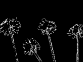
(a) $u_{1}$ (stalks)

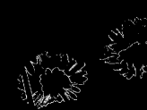
(b) $u_{2}$ (red flowers)

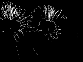
(c) $u_{3}$ (yellow flowers)

(d) $u_{4}$ (background)

Figure 1: From left to right: the initialization (white lines) of $u_{1},u_{2},u_{3}\text{ and }u_{4}$ obtained by the Multi-IGLIM.

(a) original image

(b) final contour

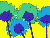
(c) final segments

Figure 2: From left to right: original image and the segmentation results.

(a) $u_{1}$ (heart)

(b) $u_{2}$ (circle)

(c) $u_{3}$ (arch)

(d) $u_{4}$ (background)

Figure 3: From left to right: the initialization of $u_{1},u_{2},u_{3}\text{ and }u_{4}$ obtained by the Multi-IGLIM.

(a) original image

(b) final contour

(c) final segments

Figure 4: From left to right: original image and the segmentation results.

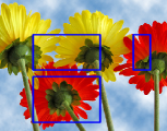
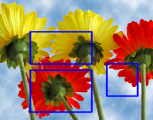
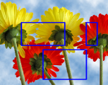
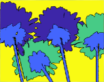
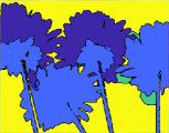
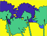
Figure 5: From top to bottom: Original images with initial contour, final contour, and final segments. All the final contours are highlighted by black lines.

Initialization	Iteration number	CPU time (s)
Column 1	19	1.001778
Column 2	38	1.994020
Column 3	182	9.263411
Multi-IGLIM	12	0.717589

Table 1: Comparison of the iteration number and CPU time for the segmentation in Fig. 5.

4.2 ICTM-LVF for images with noise

In this part, we evaluate the performance of the ICTM-LVF solver for both the CV model and the LIF model on synthetic and medical images. Comparison is made between the original ICTM and the ICTM-LVF to demonstrate the effectiveness of the ICTM-LVF in the segmentation of the images with noise. All the initial contours are given by the Multi-IGLIM.

First, we solve the CV model for the segmentation of a clean synthetic color image and its noise version. We display the segmentation results from the ICTM and the ICTM-LVF in Fig. 6. One can observe that the ICTM produces good segmentation for the clean image, but its performance on the noise image is not so appealing, while the ICTM-LVF performs quite well for both clean and noise images.

Figure 6: Comparison between the ICTM and the ICTM-LVF for solving the CV model. The first row displays the clean and noise images, the second row and the third row are the results of final contours and final segments, respectively. The first and the third columns are the results of the ICTM, while the results of the ICTM-LVF appear in the second and the fourth columns. All the final contours are highlighted by black lines.

Then, we solve the LIF model for the segmentation of images with noise at different levels with both the ICTM and the ICTM-LVF. The results are shown in Fig. 7. It can be seen that as the noise level increases, the results of the ICTM become worse, while the ICTM-LVF can still achieve relatively good segmentation.

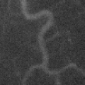
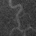
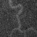
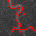
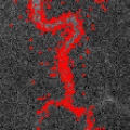
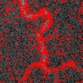
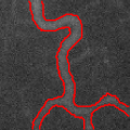
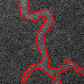
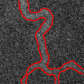
Figure 7: Comparison between the ICTM and the ICTM-LVF for solving the LIF model on the segmentation of images with the noise of different levels (The variance from the first column to the last column: 0, 50, 300, 500). From top to bottom are original images with the noise of different levels, results of the ICTM, and results of the ICTM-LVF, respectively. All the final contours are highlighted by red lines.

4.3 ICTM-LVF for real images

To further test the performance of the ICTM-LVF solver, we use it to solve the CV model for the segmentation of various real images, where the Multi-IGLIM is adopted for the initialization. The results are displayed in Fig. 8. It can be seen that our ICTM-LVF solver also performs very well on real images.

For these real images, we employ the dimension lifting technique to extract more information, which is first proposed in the SLaT model [7] and drawn on by many other models [7, 36]. The dimension lifting in this paper is to add the color information of the CIELAB color space [21, 27] to the RGB images to reflect the color information in a more comprehensive way. Consequently, the 3D vector used to present RGB information will be extended to a 6D vector.

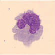
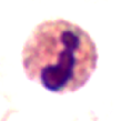
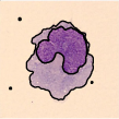
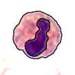
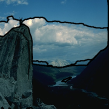
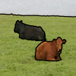
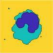
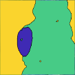
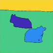
Figure 8: Experiments with the ICTM-LVF solver and the CV model on real images. From top to bottom: Original image, final contours, and final segments. All the final contours are highlighted by black lines.

4.4 Comparison between the ICTM-LVF and some state-of-art algorithms

In this part, we compare our ICTM-LVF solver with some state-of-art image segmentation algorithms on noise corrupted images and medical images in terms of segmentation performance and efficiency. The segmentation results are shown in Fig. 9 and Fig. 10. In all the experiments, the ICTM-LVF can give good results for given images while the other algorithms fail to segment all the images correctly, especially for the medical images in Fig. 10. Particularly, in the fourth row of Fig. 9, the ICTM-LVF solver with the CV model (ICTM-LVF-CV) can separate all the clouds from other objects while others can only separate the clouds with high brightness. Moreover, it can also be seen that the ICTM-LVF-CV achieves a more delicate segmentation result for the last image in Fig. 9. The results displayed in Fig. 10 indicate that compared to other algorithms, the ICTM-LVF with the LIF model (ICTM-LVF-LIF) is more suitable for images with intensity inhomogeneity. The CPU times for all algorithms are recorded in Table 2, which exhibits the high efficiency of the ICTM-LVF solver.

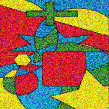
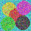
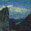
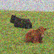
(a)Original images

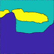
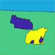
(b) SLaT

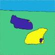
(c) Model in [36]

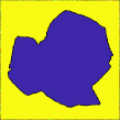
(d) Model in [8]

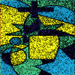
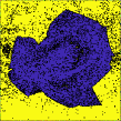
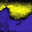
(e) ICTM-CV

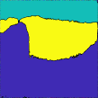
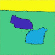
(f) ICTM-LVF-CV

Figure 9: Comparison between the ICTM-LVF-CV model and other state-of-art algorithms.

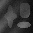
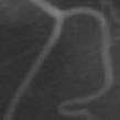
(a)Original images

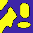
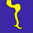
(b) SLaT

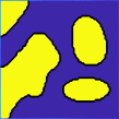
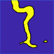
(c) Model in [36]

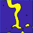
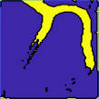
(d) Model in [8]

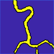
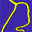
(e) ICTM-LIF

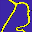
(f) ICTM-LVF-LIF

Figure 10: Comparison between the ICTM-LVF-LIF model and other state-of-art algorithms.

Images		SLaT	Model in [36]	Model in [8]	ICTM	ICTM-LVF
Fig. 9	Row1	2.035450	4.180187	2.815690	0.937057	0.969474
	Row2	0.485363	0.500887	0.462177	0.298151	0.316960
	Row3	1.781461	1.205533	2.006805	0.517074	0.529115
	Row4	9.804071	18.852447	6.061458	2.195570	4.333940
	Row5	8.487740	14.231849	7.372541	5.178055	6.885624
Fig. 10	Row1	0.566980	1.065398	0.743467	0.172654	0.233498
	Row2	0.372138	1.007371	0.384031	0.096292	0.166943
	Row3	0.711676	1.048547	0.723667	0.192009	0.282930
	Row4	1.066218	1.171380	0.964410	0.261146	0.465101

Table 2: CPU time(s) for experiments in Fig. 9 and Fig. 10.

5 Conclusion

We propose a new framework on active contour models for the multi-phase image segmentation. This framework consists of a novel energy with a local variance force term, an effective initialization method (Multi-IGLIM), and an efficient energy-decaying algorithm (ICTM-LVF) based on the modification of the ICTM. The proposed Multi-IGLIM and the ICTM-LVF solver can greatly improve the robustness of active contour models to the initialization and noise. Experiments show that compared to some state-of-the-art methods, the proposed framework has better performance in terms of the segmentation quality and the running time, even applied to images with severe intensity inhomogeneity and strong noise.

References

- [1] S. Abburu and S. Babu Golla, Satellite image classification methods and techniques: A review, International Journal of Computer Applications, 119 (2015), pp. 20–25.
- [2] F. Akram, M. A. Garcia, and D. Puig, Active contours driven by local and global fitted image models for image segmentation robust to intensity inhomogeneity, PloS one, 12 (2017), p. e0174813.
- [3] E. Bae and X.-C. Tai, Efficient global minimization methods for image segmentation models with four regions, Journal of Mathematical Imaging and Vision, 51 (2015), pp. 71–97.
- [4] E. Bae, J. Yuan, and X.-C. Tai, Global minimization for continuous multiphase partitioning problems using a dual approach, International Journal of Computer Vision, 92 (2011), pp. 112–129.
- [5] X. Bresson, S. Esedoḡlu, P. Vandergheynst, J.-P. Thiran, and S. Osher, Fast global minimization of the active contour/snake model, Journal of Mathematical Imaging and vision, 28 (2007), pp. 151–167.
- [6] E. S. Brown, T. F. Chan, and X. Bresson, A convex relaxation method for a class of vector-valued minimization problems with applications to Mumford-Shah segmentation, UCLA CAM report, 10 (2010).
- [7] X. Cai, R. Chan, M. Nikolova, and T. Zeng, A three-stage approach for segmenting degraded color images: Smoothing, lifting and thresholding (SLaT), Journal of Scientific Computing, 72 (2017), pp. 1313–1332.
- [8] X. Cai, R. Chan, and T. Zeng, A two-stage image segmentation method using a convex variant of the Mumford–Shah model and thresholding, SIAM Journal on Imaging Sciences, 6 (2013), pp. 368–390.
- [9] V. Caselles, R. Kimmel, and G. Sapiro, Geodesic active contours, International Journal of Computer Vision, 22 (1997), pp. 61–79.
- [10] R. Chan, A. Lanza, S. Morigi, and F. Sgallari, Convex non-convex image segmentation, Numerische Mathematik, 138 (2018), pp. 635–680.
- [11] T. F. Chan, S. Esedoglu, and M. Nikolova, Algorithms for finding global minimizers of image segmentation and denoising models, SIAM Journal on Applied Mathematics, 66 (2006), pp. 1632–1648.
- [12] T. F. Chan and L. A. Vese, Active contours without edges, IEEE Transactions on Image Processing, 10 (2001), pp. 266–277.
- [13] L. Guo, Y. Liu, Y. Wang, Y. Duan, and X.-C. Tai, Learned snakes for 3D image segmentation, Signal Processing, 183 (2021), p. 108013.
- [14] Y. M. Jung, S. H. Kang, and J. Shen, Multiphase image segmentation via Modica–Mortola phase transition, SIAM Journal on Applied Mathematics, 67 (2007), pp. 1213–1232.
- [15] M. Kass, A. Witkin, and D. Terzopoulos, Snakes: Active contour models, International Journal of Computer Vision, 1 (1988), pp. 321–331.
- [16] C. Li, R. Huang, Z. Ding, J. C. Gatenby, D. N. Metaxas, and J. C. Gore, A level set method for image segmentation in the presence of intensity inhomogeneities with application to MRI, IEEE Transactions on Image Processing, 20 (2011), pp. 2007–2016.
- [17] C. Li, C.-Y. Kao, J. C. Gore, and Z. Ding, Implicit active contours driven by local binary fitting energy, in 2007 IEEE Conference on Computer Vision and Pattern Recognition, 2007, pp. 1–7.
- [18] C. Li, C.-Y. Kao, J. C. Gore, and Z. Ding, Minimization of region-scalable fitting energy for image segmentation, IEEE Transactions on Image Processing, 17 (2008), pp. 1940–1949.
- [19] Y. Li and J. Kim, Multiphase image segmentation using a phase-field model, Computers and Mathematics with Applications, 62 (2011), pp. 737–745.
- [20] C. Liu, Z. Qiao, and Q. Zhang, Two-phase segmentation for intensity inhomogeneous images by the Allen–Cahn local binary fitting model, SIAM Journal on Scientific Computing, 44 (2022), pp. B177–B196.
- [21] Q.-T. Luong, Color in computer vision, in Handbook of pattern recognition and computer vision, World Scientific, 1993, pp. 311–368.
- [22] J. Ma, D. Wang, X.-P. Wang, and X. Yang, A characteristic function-based algorithm for geodesic active contours, SIAM Journal on Imaging Sciences, 14 (2021), pp. 1184–1205.
- [23] L. Min, Q. Cui, Z. Jin, and T. Zeng, Inhomogeneous image segmentation based on local constant and global smoothness priors, Digital Signal Processing, 111 (2021), p. 102989.
- [24] A. Mitiche and I. B. Ayed, Variational and level set methods in image segmentation, vol. 5, Springer Science & Business Media, 2010.
- [25] S. Niu, Q. Chen, L. De Sisternes, Z. Ji, Z. Zhou, and D. L. Rubin, Robust noise region-based active contour model via local similarity factor for image segmentation, Pattern Recognition, 61 (2017), pp. 104–119.
- [26] S. Osher and J. A. Sethian, Fronts propagating with curvature-dependent speed: Algorithms based on Hamilton-Jacobi formulations, Journal of Computational Physics, 79 (1988), pp. 12–49.
- [27] G. Paschos, Perceptually uniform color spaces for color texture analysis: an empirical evaluation, IEEE Transactions on Image Processing, 10 (2001), pp. 932–937.
- [28] D. L. Pham, C. Xu, and J. L. Prince, Current methods in medical image segmentation, Annual Review of Biomedical Engineering, 2 (2000), pp. 315–337.
- [29] T. Pock, D. Cremers, H. Bischof, and A. Chambolle, An algorithm for minimizing the mumford-shah functional, in 2009 IEEE 12th International Conference on Computer Vision, IEEE, 2009, pp. 1133–1140.
- [30] Z. Qiao and Q. Zhang, Two-phase image segmentation by the Allen-Cahn equation and a nonlocal edge detection operator, Numerical Mathematics: Theory, Methods and Applications, Accepted, 2022, https://arxiv.org/abs/2104.08992.
- [31] Y. Song, G. Peng, D. Sun, and X. Xie, Active contours driven by gaussian function and adaptive-scale local correntropy-based k-means clustering for fast image segmentation, Signal Processing, 174 (2020), p. 107625.
- [32] L. A. Vese and T. F. Chan, A multiphase level set framework for image segmentation using the Mumford and Shah model, International Journal of Computer Vision, 50 (2002), pp. 271–293.
- [33] D. Wang, H. Li, X. Wei, and X. P. Wang, An efficient iterative thresholding method for image segmentation, Journal of Computational Physics, 350 (2017), pp. 657–667.
- [34] D. Wang and X. P. Wang, The iterative convolution-thresholding method (ICTM) for image segmentation, arXiv preprint arXiv:1904.10917, (2019). https://arxiv.org/pdf/1904.10917.pdf.
- [35] L. Wang, C. Li, Q. Sun, D. Xia, and C.-Y. Kao, Active contours driven by local and global intensity fitting energy with application to brain mr image segmentation, Computerized Medical Imaging and Graphics, 33 (2009), pp. 520–531.
- [36] T. Wu, X. Gu, J. Shao, R. Zhou, and Z. Li, Color image segmentation based on a convex k-means approach, IET Image Process, 15 (2021), pp. 1596–1606.
- [37] T. Wu, X. Gu, Y. Wang, and T. Zeng, Adaptive total variation based image segmentation with semi-proximal alternating minimization, Signal Processing, 183 (2021), p. 108017.
- [38] T. Wu and J. Shao, Non-convex and convex coupling image segmentation via TGpV regularization and thresholding, Advances in Applied Mathematics and Mechanics, 12 (2020), pp. 849–878.
- [39] T. Wu, J. Shao, X. Gu, M. K. Ng, and T. Zeng, Two-stage image segmentation based on nonconvex - approximation and thresholding, Applied Mathematics and Computation, 403 (2021), p. 126168.
- [40] W. Yang, Z. Huang, and W. Zhu, Image Segmentation Using the Cahn–Hilliard Equation, Journal of Scientific Computing, 79 (2019), pp. 1057–1077.
- [41] D. Zosso, J. An, J. Stevick, N. Takaki, M. Weiss, L. S. Slaughter, H. H. Cao, P. S. Weiss, and A. L. Bertozzi, Image segmentation with dynamic artifacts detection and bias correction, Inverse Problems and Imaging, 11 (2017), pp. 577–600.