Selection and parallel trends

Abstract

We study the role of selection into treatment in difference-in-differences (DiD) designs. We derive necessary and sufficient conditions for parallel trends assumptions under general classes of selection mechanisms. These conditions characterize the empirical content of parallel trends. For settings where the necessary conditions are questionable, we propose tools for selection-based sensitivity analysis. We also provide templates for justifying DiD in applications with and without covariates. A reanalysis of the causal effect of NSW training programs demonstrates the usefulness of our selection-based approach to sensitivity analysis.

Keywords: causal inference, conditional parallel trends, covariates, difference-in-differences, selection mechanism, sensitivity analysis, time-invariant and time-varying unobservables, treatment effects

JEL Codes: C21, C23

…while the new papers [in the DiD literature] clarify very well the statistical assumptions needed for estimation, effective use of these methods also requires being able to understand what the threats to these assumptions are in different contexts, and to make a plausible rhetorical argument as to why we should think the assumptions hold.
— David McKenzie, World Bank Development Impact Blog (McKenzie,, 2022)

1 Introduction

Difference-in-differences (DiD) is a widely-used causal inference method. One of the perceived advantages of DiD is that it does not require explicit assumptions on how units select into treatment but instead relies on parallel trends assumptions. However, when justifying DiD in empirical applications, researchers often argue that the treatment is “quasi-randomly” assigned. Although these discussions allude to selection mechanisms, they are often not explicit about what constitutes “quasi-random” assignment, arguably due to the lack of formal guidance.

In this paper, we study parallel trends assumptions through the lens of selection. We have three goals: (i) characterize the empirical content of parallel trends; (ii) propose new approaches to sensitivity analysis that leverage contextual knowledge about selection; (iii) provide templates for justifying parallel trends in practice with and without covariates. Since DiD is applied in a myriad of empirical contexts, we consider general classes of selection mechanisms that accommodate selection on time-invariant unobservables (“fixed effects”), selection on untreated potential outcomes, selection on treatment effects (Roy-style selection), and other economic models of selection.

We first derive necessary and sufficient conditions for parallel trends. These conditions are helpful for understanding the threats to the identification assumptions underlying DiD, which in turn is essential for an “effective use of these methods,” as emphasized by McKenzie, (2022)’s quote. We first consider a scenario where researchers are not willing to restrict the selection mechanism. We show that absent any restrictions on selection, parallel trends holds if and only if the untreated potential outcome is constant across time up to deterministic mean shifts. This condition is restrictive in many applications: it essentially rules out time-varying unobservables.

This negative result motivates restricting the selection mechanism. We derive necessary conditions for parallel trends under restrictions that can be motivated based on classical examples of selection as well as the information sets available to units at the time of the decision. First, if the units only select on information from the pre-treatment period (imperfect foresight), parallel trends implies that the untreated potential outcome satisfies a martingale property. Second, if the units select into treatment based on fixed effects, so that selection does not depend on time-varying unobservables, parallel trends implies a stationarity restriction on the mean of the untreated potential outcome conditional on the fixed effects. Under additional assumptions, these two necessary conditions are also sufficient for parallel trends. Taken together, our necessary and sufficient conditions imply that researchers relying on parallel trends assumptions face a trade-off between restrictions on selection into treatment and restrictions on the time-series properties of the outcomes.

Our necessary conditions for parallel trends motivate a selection-based approach to sensitivity analysis. Suppose, for example, that the units have imperfect foresight such that selection depends on pre-treatment unobservables. In these settings, researchers may be willing to rule out parallel trends violations due to selection on post-treatment unobservables. Deviations from the martingale property of the untreated potential outcomes can still threaten the validity of the parallel trends assumption, however. We therefore characterize the average treatment effect on the treated (ATT) under violations of the martingale property in settings with and without additional pre-treatment periods. This characterization allows researchers to leverage contextual knowledge about selection to perform sensitivity analyses, to compute bounds on the ATT, and to construct robust confidence intervals.

We also offer a menu of primitive sufficient conditions for justifying parallel trends in empirical applications, building on our necessary conditions. These conditions constitute theory-based templates for making “plausible rhetorical arguments as to why we should think the [parallel trends] assumptions hold” (McKenzie,, 2022). More specifically, these conditions can be used to justify parallel trends based on contextual knowledge about selection, such as what units select on and what information sets are available to them at the time of the selection decision. Our primitive sufficient conditions explicitly allow for selection on time-invariant and time-varying unobservables, thus formalizing what one might mean by “quasi-random” assignment in the context of DiD analyses.

Our necessary and sufficient conditions generalize directly to settings with covariates. They demonstrate that parallel trends assumptions conditional on the trajectory of covariates imply combinations of time homogeneity and separability restrictions on how the covariates enter the outcome model, even when selection only depends on time-invariant unobservables. We therefore consider a weaker conditional parallel trends assumption, designed specifically to accommodate nonseparability between observables and unobservables in the outcome model. We provide a menu of sufficient conditions for this weaker conditional parallel trends assumption and establish connections between these selection-based conditions and identification assumptions in the literature on nonseparable panel data models.

We illustrate the usefulness of the selection-based approach to sensitivity analysis by reanalyzing the causal effect of the NSW training programs using DiD methods. Selection on unobservables in the pre-treatment period (imperfect foresight) is a major concern when evaluating training programs. Our sensitivity analysis allows us to assess the sensitivity of DiD with respect to violations of the martingale assumption. We find that the DiD estimates without covariates not only differ substantially from the experimental benchmark, but are also very sensitive to violations of the martingale property and thus parallel trends. Incorporating covariates into the analysis reduces the estimated bias relative to the experimental benchmark and also renders the results more robust.

Related literature.

This paper contributes to several branches of the literature on causal inference using panel data. Our first contribution is to the classical literature on canonical DiD setups. See, e.g., Ashenfelter, (1978), Ashenfelter and Card, (1985), Heckman and Robb, (1985), Card, (1990), Card and Krueger, (1994), Meyer et al., (1995), and Angrist and Krueger, (1999) for early developments, and Section 2 of Lechner, (2010) for a historical perspective. Our contribution is to provide foundations for the parallel trends assumption to hold in non-experimental settings, where selection into treatment may depend on time-invariant and time-varying unobservables.

Our second contribution is to the more recent literature on DiD methods. See, e.g., de Chaisemartin and D’Haultfœuille, (2023) and Roth et al., (2023) for surveys. Our paper is most closely related to Roth and Sant’Anna, (2023), Arkhangelsky et al., (2021), and Arkhangelsky and Imbens, (2022), though our focus greatly differs from theirs. Roth and Sant’Anna, (2023) discuss necessary and sufficient conditions under which the parallel trends assumption is satisfied for all (monotonic) transformations of the untreated potential outcome. We, on the other hand, take the outcome model (and thus the specific transformation) as given and study the connection between parallel trends and selection into treatment. Arkhangelsky et al., (2021) and Arkhangelsky and Imbens, (2022) propose doubly robust estimation methods that leverage restrictions on outcome models and/or selection models with unconfoundedness-type restrictions; see also Athey et al., (2021). Our results complement theirs as we maintain the parallel trends assumption and discuss the types of restrictions on selection compatible with it. Moreover, our analysis shows that parallel trends is compatible with various types of selection on unobservables, unlike standard unconfoundedness assumptions (e.g., Imbens,, 2004; Imbens and Wooldridge,, 2009).

Our third contribution is to the literature on sensitivity analysis, partial identification, and robust inference under violations of parallel trends. Our approach differs from the methods in Manski and Pepper, (2018), Ban and Kédagni, (2023), and Rambachan and Roth, (2023) in that we explicitly rely on assumptions on selection that can be motivated from contextual knowledge about a given empirical setting. Our sensitivity analysis can be performed with and without additional pre-treatment periods. Relative to the existing literature, we use the additional pre-treatment periods to learn about the time-series properties of the outcomes, instead of directly making assumptions about how the parallel trends violation changes over time. For these reasons, our sensitivity analysis complements these existing approaches. Our selection-based approach also differs from the analysis by Marx et al., (2023). They derive partial identification results under monotone treatment selection assumptions on the untreated potential outcome, which they motivate using an economic model of learning with binary outcomes. By contrast, we directly exploit restrictions on the selection mechanism.

Our fourth contribution is to the literature imposing explicit selection and/or outcome models to develop and compare different methods for estimating treatment effects, including DiD (e.g., Ashenfelter and Card,, 1985; Heckman and Robb,, 1985; Card and Hyslop,, 2005; Chabé-Ferret,, 2015; Blundell and Dias,, 2009; de Chaisemartin and D’Haultfœuille,, 2018; Verdier,, 2020; Marx et al.,, 2023). These selection mechanisms were developed for economic models, some of which are tailored to applications such as job training and technology adoption. Our results complement this strand of the literature in several ways. First, our necessary and sufficient conditions are derived for general selection and outcome models that nest models considered in this literature. Our conditions thus clarify trade-offs between assumptions on selection and time-varying unobservables that are relevant for those models. Second, our primitive sufficient conditions nest several of the existing application-specific restrictions. Third, we provide results for general nonseparable models and clarify the role of covariates in the context of parallel trends assumptions. It is worth noting that while most papers in this literature examine sharp DiD designs, as we do, de Chaisemartin and D’Haultfœuille, (2018) and Marx et al., (2023) also consider fuzzy DiD designs.

Finally, we establish an explicit connection between DiD and the literature on nonseparable panel models. A strand of this literature has analyzed the identification of average effects either by allowing for fixed effects and imposing time homogeneity (e.g. Hoderlein and White,, 2012; Chernozhukov et al.,, 2013) or restricting individual heterogeneity via nonparametric correlated random effects assumptions (e.g. Altonji and Matzkin,, 2005; Bester and Hansen,, 2009). We show that our sufficient conditions for parallel trends imply combinations of time homogeneity and (correlated) random effects restrictions. Our results demonstrate how restrictions on the selection mechanism can be used to justify identification assumptions in the nonseparable panel literature.

Notation. For a random vector $W_{it}$, where $i=1,\dots,n$ and $t=1,2$, we denote its time series by $W_{i}\equiv(W_{i1},W_{i2})$. We use $F_{W}$ to denote the distribution of the random vector $W$. Let $f(z,w)$ be a function defined on $\mathcal{Z}\times\mathcal{W}$. We say that $f(z,w)$ is a trivial function of $w$ if $f(z,w)=f(z,w^{\prime})=h(z)$ for all $z\in\mathcal{Z}$, $w\neq w^{\prime}$, and $(w,w^{\prime})\in\mathcal{W}^{2}$. We say that $f(z,w)$ is a symmetric function in $z$ and $w$ if $f(z,w)=f(w,z)$ for all $(z,w)\in\mathcal{Z}\times\mathcal{W}$. For a vector $W_{i}$, $W_{i}^{j}$ is the $j^{th}$ element of $W_{i}$. We use the notation $\overset{d}{=}$ to denote equality of distribution. For random variables, $X_{i}$, $Z_{i}$, and $W_{i}$, $Z_{i}|W_{i},X_{i}\overset{d}{=}Z_{i}|X_{i},W_{i}$ denotes that $F_{Z_{i}|W_{i},X_{i}}(z|w,x)=F_{Z_{i}|X_{i},W_{i}}(z|w,x)$ for $(z,w,x)\in\mathcal{Z}\times\mathcal{W}\times\mathcal{X}$.

2 Setup, selection mechanism, and examples

We consider the classical DiD setup with two groups and two periods and abstract from covariates. We discuss the role of covariates in Section 6 and generalize our results to DiD designs with multiple groups and multiple periods in Appendix C.2. Let $D_{it}$ and $Y_{it}$ denote the treatment status and outcome for unit $i\in\{1,\dots,n\}$ in period $t\in\{1,2\}$. Here the index $i$ refers to the unit making the decision to select into treatment. This could be an individual or a more aggregate administrative unit, such as county or state. See Appendix B for a discussion of DiD designs where the data are available at the disaggregate level (e.g., individual level), while the selection decision is made at the aggregate level (e.g., state level). The treatment group ($G_{i}=1$) selects the treatment path $D_{i}=(0,1)$; the control group ($G_{i}=0$) selects $D_{i}=(0,0)$. The potential outcomes with and without the treatment are $Y_{it}(1)$ and $Y_{it}(0)$, respectively.

We consider the standard parallel trends assumption. Throughout the paper, we assume that all relevant moments exist and $\{Y_{i1}(0),Y_{i2}(0),G_{i}\}$ is i.i.d. across $i$.

Assumption PT.

The (unconditional) parallel trends assumption holds:

$$E[Y_{i2}(0)-Y_{i1}(0)|G_{i}=1]=E[Y_{i2}(0)-Y_{i1}(0)|G_{i}=0].$$

Under Assumption PT, the average treatment effect on the treated group in period $t=2$, $\operatorname{ATT}\equiv E[Y_{i2}(1)-Y_{i2}(0)|G_{i}=1]$, is identified from the “difference-in-differences” as follows:

$$\operatorname{ATT}=E[Y_{i2}-Y_{i1}|G_{i}=1]-E[Y_{i2}-Y_{i1}|G_{i}=0]\equiv\operatorname{DiD}.$$

We work with a general nonseparable model for $Y_{it}(0)$,

$$Y_{it}(0)=\xi_{t}(\alpha_{i},\varepsilon_{it}),\quad i=1,\dots,n,\quad t=1,2,$$ (1)

where $\alpha_{i}$, $\varepsilon_{i1}$, and $\varepsilon_{i2}$ are finite-dimensional vector-valued random variables, and $\xi_{t}(\cdot)$ is an unrestricted time-varying function. The outcome model (1), while not imposing any restrictions on $Y_{it}(0)$, allows us to distinguish between time-invariant and time-varying unobservables. This is necessary to define selection mechanisms that can directly depend on these unobservables. If, instead, we were to work directly with potential outcomes, this would rule out important examples of selection mechanisms such as selection on time-invariant unobservables (e.g., Ashenfelter and Card,, 1985).

We consider a general class of selection mechanisms in which units select into treatment based on $(\alpha_{i},\varepsilon_{i1},\varepsilon_{i2})$ as well as a vector of additional time-invariant and time-varying random variables, $(\nu_{i},\eta_{i1},\eta_{i2})$,

$$G_{i}=g(\alpha_{i},\varepsilon_{i1},\varepsilon_{i2},\nu_{i},\eta_{i1},\eta_{i2}).$$ (2)

This selection mechanism accommodates many different types of selection, including random assignment, selection on fixed effects, selection on untreated potential outcomes, selection on treatment effects, and other economic models of selection (e.g. Heckman and Robb,, 1985; Chabé-Ferret,, 2015; Marx et al.,, 2023). Note that since $G_{i}=D_{i2}$, $g(\cdot)$ can be equivalently viewed as the selection mechanism for $D_{i2}$. Let $\mathcal{G}_{\text{all}}$ denote the set of all selection mechanisms $g(\cdot)$ mapping from the support of the unobservables to $\{0,1\}$.

Throughout the paper, we will come back to the following three leading examples of selection, specifically selection on outcomes, on treatment effects, and on fixed effects.

Example 2.1 (Selection on outcomes).

We consider a class of threshold-crossing selection mechanisms, generalizing the selection mechanisms analyzed in Ashenfelter and Card, (1985), who study the effect of training programs on earnings. Let $\omega_{i}$ denote the information set available to the units when deciding whether to participate in the training program and consider the following mechanism,

$$G_{i}=1\left\{E[Y_{i1}(0)+\beta Y_{i2}(0)|\omega_{i}]\leq E[C_{i2}|\omega_{i}]\right\},$$ (3)

where $\beta\in[0,1]$ is a discount factor, $G_{i}$ indicates participation in a job training program, $Y_{it}(0)$ denotes untreated potential earnings, $C_{i2}$ is the individual-specific threshold, which is assumed to be an element of $\eta_{i2}$. The selection mechanism (3) can be expressed as $G_{i}=\check{g}(\omega_{i})$ and is therefore a special case of the mechanism (2) if $\omega_{i}$ is a subvector of $(\alpha_{i},\varepsilon_{i1},\varepsilon_{i2},\nu_{i},\eta_{i1},\eta_{i2})$. ∎

Example 2.2 (Selection on treatment effects (Roy-style selection)).

Suppose that units select into the treatment if the expected gains from treatment given the information set $\omega_{i}$, $E[Y_{i2}(1)-Y_{i2}(0)|\omega_{i}]$, exceed the expected cost of treatment, $E[C_{i2}|\omega_{i}]$,

$$G_{i}=1\{E[Y_{i2}(1)-Y_{i2}(0)|\omega_{i}]\geq E[C_{i2}|\omega_{i}]\}.$$ (4)

The selection mechanism (4) is again a special case of mechanism (2) if $\omega_{i}$ is a subvector of $(\alpha_{i},\varepsilon_{i1},\varepsilon_{i2},\nu_{i},\eta_{i1},\eta_{i2})$. This example shows that it is important to allow $g(\cdot)$ to depend on a vector of additional unobservables, such that we can allow $\eta_{i2}$ (and thus the information set) to include $(Y_{i2}(1),C_{i2})$. ∎

Example 2.3 (Selection on fixed effects).

DiD methods have traditionally been motivated using two-way fixed effects models. Fixed effects assumptions allow for unrestricted dependence between time-invariant unobservables and the regressors, thereby implicitly allowing for selection on time-invariant unobservables. The general selection mechanism (2) accommodates this classical type of selection if $g(\cdot)$ is a trivial function of $(\varepsilon_{i1},\varepsilon_{i2},\eta_{i1},\eta_{i2})$. A simple example is $G_{i}=1\{\alpha_{i}\leq c\}$, which corresponds to the selection mechanism on p.650 in Ashenfelter and Card, (1985). ∎

Remark 2.1 (Parallel trends and functional form).

Throughout this paper, we take the functional form of the outcome as given. We thereby abstract from the issues arising from the sensitivity of DiD to functional form specification; see Roth and Sant’Anna, (2023) for a discussion. ∎

3 Necessary and sufficient conditions for parallel trends

3.1 No restrictions on selection

To better understand the implications of parallel trends, we derive necessary and sufficient conditions for this assumption. We start by analyzing a scenario where researchers are not willing to make any assumptions on the selection mechanism so that parallel trends needs to hold for all selection mechanisms.

To ensure non-degeneracy of the selection mechanisms we use to derive necessary and sufficient conditions for parallel trends, we impose the following weak regularity condition.

Assumption SEL.

There exists a component of $\nu_{i}$, labeled $\nu_{i}^{1}$ (w.l.o.g.), such that $\nu_{i}^{1}\perp\!\!\!\perp(\alpha_{i},\varepsilon_{i1},\varepsilon_{i2})$ and $P(\nu_{i}^{1}>c)\in(0,1)$ for some $c\in\mathbb{R}$.

Assumption SEL requires that one of the unobservables in the selection mechanism is independent of the unobservable determinants of $Y_{it}(0)$ for $t=1,2$. Intuitively, this condition just requires that there is some random shock affecting a unit’s decision to select into treatment.

The following proposition presents a necessary and sufficient condition for parallel trends holding for all selection mechanisms. To simplify exposition, we use $\dot{Y}_{it}(0)$ to denote the centered potential outcome without the treatment, $\dot{Y}_{it}(0)\equiv Y_{it}(0)-E[Y_{it}(0)]$, for $t=1,2$.

Proposition 3.1 (Necessary and sufficient condition for $g\in\mathcal{G}_{\text{all}}$).

Suppose that Assumption SEL holds and either $P(\dot{Y}_{i2}(0)>\dot{Y}_{i1}(0))<1$ or $P(\dot{Y}_{i2}(0)<\dot{Y}_{i1}(0))<1$. Then, Assumption PT holds for all $g\in\mathcal{G}_{\text{all}}$ satisfying $P(G_{i}=1)\in(0,1)$ if and only if $\dot{Y}_{i1}(0)=\dot{Y}_{i2}(0)$ a.s.

Together with Assumption SEL, $P(\dot{Y}_{i2}(0)>\dot{Y}_{i1}(0))<1$ (or $P(\dot{Y}_{i2}(0)<\dot{Y}_{i1}(0))<1$) implies that the selection mechanism we use to prove the “only-if” direction of the proof is non-degenerate. These conditions are not restrictive in applications since they merely rule out that the supports of the demeaned potential outcomes are disjoint.

To interpret the necessary and sufficient condition in Proposition 3.1, it is helpful to rewrite it as

$$Y_{i2}(0)=Y_{i1}(0)+E[Y_{i2}(0)-Y_{i1}(0)].$$

This shows that absent any restrictions on selection, parallel trends implies that the potential outcomes are constant over time, except for common mean shifts. Given that this condition is implausible in many applications, we consider restricted classes of selection mechanisms in Section 3.2.

3.2 Restricted selection mechanisms

Motivated by Proposition 3.1, we consider two restricted classes of selection mechanisms. These classes of mechanisms are directly related to and motivated by the information sets available to the units when making the decision to select into the treatment.

First, we examine a class of selection mechanisms in which individuals have imperfect foresight so that selection depends on the time-invariant and pre-treatment unobservables,

$$\mathcal{G}_{\text{if}}=\{g\in\mathcal{G}_{\text{all}}:g(a,e_{1},e_{2},v,t_{1},t_{2})\text{ is a trivial function of }(e_{2},t_{2})\}.$$

In Example 2.1, $\mathcal{G}_{\text{if}}$ captures settings where individuals know their permanent income component, $\alpha_{i}$, and the pre-treatment idiosyncratic earnings shock, $\varepsilon_{i1}$, but not the unobservables from the post-treatment period, specifically $\varepsilon_{i2}$ and $C_{i2}$. For empirical evidence on the heterogeneity in income uncertainty faced by different individuals, see, e.g., Arellano et al., (2022). In Example 2.2, assuming that $g\in\mathcal{G}_{\text{if}}$ requires that individuals do not know their treatment effects, $Y_{i2}(1)-Y_{i2}(0)$, and costs, $C_{i2}$, while their information set can contain all time-invariant and pre-treatment unobservables $(\alpha_{i},\varepsilon_{i1},\nu_{i},\eta_{i1})$.

Second, we consider a class of mechanisms where selection only depends on the fixed effects $(\alpha_{i},\nu_{i})$,

$$\mathcal{G}_{\text{fe}}=\{g\in\mathcal{G}_{\text{all}}:g(a,e_{1},e_{2},v,t_{1},t_{2})\text{ is a trivial function of }(e_{1},e_{2},t_{1},t_{2})\}.$$

The class of selection mechanisms $\mathcal{G}_{\text{fe}}$ captures the classical scenario of selection on fixed effects. Assuming that $g\in\mathcal{G}_{\text{fe}}$ is plausible if either the units’ information set only contains the time-invariant unobservables in Examples 2.1 and 2.2, so that $\omega_{i}=(\alpha_{i},\nu_{i})$, or if selection is directly based on fixed effects as in Example 2.3.

The next two propositions provide necessary conditions for parallel trends when the selection mechanism belongs to $\mathcal{G}_{\text{if}}$ and $\mathcal{G}_{\text{fe}}$, respectively.

Proposition 3.2 (Necessary condition for $g\in\mathcal{G}_{\text{if}}$).

Suppose that Assumption SEL holds and either $P(E[\dot{Y}_{i2}(0)|\alpha_{i},\varepsilon_{i1}]>\dot{Y}_{i1}(0))<1$ or $P(E[\dot{Y}_{i2}(0)|\alpha_{i},\varepsilon_{i1}]<\dot{Y}_{i1}(0))<1$. If Assumption PT holds for all $g\in\mathcal{G}_{\text{if}}$ satisfying $P(G_{i}=1)\in(0,1)$, then $E[\dot{Y}_{i2}(0)|\alpha_{i},\varepsilon_{i1}]=\dot{Y}_{i1}(0)$ a.s.

Proposition 3.3 (Necessary condition for $g\in\mathcal{G}_{\text{fe}}$).

Suppose that Assumption SEL holds and either $P(E[\dot{Y}_{i2}(0)|\alpha_{i}]>E[\dot{Y}_{i1}(0)|\alpha_{i}])<1$ or $P(E[\dot{Y}_{i2}(0)|\alpha_{i}]<E[\dot{Y}_{i1}(0)|\alpha_{i}])<1$. If Assumption PT holds for all $g\in\mathcal{G}_{\text{fe}}$ satisfying $P(G_{i}=1)\in(0,1)$, then $E[\dot{Y}_{i1}(0)|\alpha_{i}]=E[\dot{Y}_{i2}(0)|\alpha_{i}]$ a.s.

The two propositions demonstrate that while parallel trends is compatible with the presence of time-varying unobservables under the restricted classes of selection mechanisms, it implies time-series restrictions on $\dot{Y}_{it}(0)$. It is helpful to interpret the necessary conditions under a simple linear two-way model for $Y_{it}(0)$,

$$Y_{it}(0)=\alpha_{i}+\lambda_{t}+\varepsilon_{it},\quad E[\varepsilon_{it}]=0.$$ (5)

Under this model, the necessary condition in Proposition 3.2 becomes $E[\varepsilon_{i2}|\alpha_{i},\varepsilon_{i1}]=\varepsilon_{i1}$, a martingale-type property that implies $\varepsilon_{i2}=\varepsilon_{i1}+\zeta_{i2}$, where $\zeta_{i2}$ is an innovation satisfying $E[\zeta_{i2}|\alpha_{i},\varepsilon_{i1}]=0$. The necessary condition in Proposition 3.3 simplifies to $E[\varepsilon_{i1}|\alpha_{i}]=E[\varepsilon_{i2}|\alpha_{i}]$, a time homogeneity assumption on the conditional mean. In general, the stability of the conditional mean is implied by (and weaker than) the textbook strict exogeneity assumption, $E[\varepsilon_{it}|G_{i},\alpha_{i}]=0$, since in our framework selection may depend on additional unobservables $(\nu_{i},\eta_{i1},\eta_{i2})$.

The necessary conditions in Propositions 3.2 and 3.3 do not imply parallel trends in general due to the presence of the additional unobservables $(\nu_{i},\eta_{i1},\eta_{i2})$. The following proposition provides simple sufficient conditions in terms of the conditional distribution of the additional unobservables entering the selection mechanism under which these necessary conditions are also sufficient.

Proposition 3.4 (Sufficient conditions for $\mathcal{G}_{\text{if}}$ and $\mathcal{G}_{\text{fe}}$).

Suppose that $P(G_{i}=1)\in(0,1)$.

1. Suppose that $g\in\mathcal{G}_{\text{if}}$. If $(\nu_{i},\eta_{i1})|\alpha_{i},\varepsilon_{i1},\varepsilon_{i2}\overset{d}{=}(\nu_{i},\eta_{i1})|\alpha_{i},\varepsilon_{i1}$, then $E[\dot{Y}_{i2}(0)|\alpha_{i},\varepsilon_{i1}]=\dot{Y}_{i1}(0)$ implies Assumption PT.

2. Suppose that $g\in\mathcal{G}_{\text{fe}}$. If $\nu_{i}|\alpha_{i},\varepsilon_{i1},\varepsilon_{i2}\overset{d}{=}\nu_{i}|\alpha_{i}$, then $E[\dot{Y}_{i1}(0)|\alpha_{i}]=E[\dot{Y}_{i2}(0)|\alpha_{i}]$ implies Assumption PT.

Taken together, our necessary conditions demonstrate trade-offs between restrictions on selection into treatment and restrictions on the time-series properties of potential outcomes. In particular, these results highlight the role of restrictions on time-varying unobservables, either in terms of how they vary over time or how they determine selection. As a result, researchers using DiD approaches cannot avoid making meaningful and nontrivial assumptions on selection and time-varying unobservables.

3.3 Necessary and sufficient conditions: extensions

Here, we briefly summarize two extensions. See Appendix C for details.

3.3.1 Parallel trends for any distribution

In Appendix C.1, we provide necessary and sufficient conditions for an alternative scenario where researchers are not willing to restrict the distribution of unobservables. Specifically, suppose researchers want parallel trends to hold for all $F_{\alpha_{i},\varepsilon_{i1},\varepsilon_{i2},\nu_{i},\eta_{i1},\eta_{i2}}\in\mathcal{F}$, where $\mathcal{F}$ is a complete class of distributions. We show that Assumption PT holds for all $F_{\alpha_{i},\varepsilon_{i1},\varepsilon_{i2},\nu_{i},\eta_{i1},\eta_{i2}}\in\mathcal{F}$ if and only if

$$P(G_{i}=1|\alpha_{i},\varepsilon_{i1},\varepsilon_{i2})=P(G_{i}=1)\text{ a.s.\ for all }F_{\alpha_{i},\varepsilon_{i1},\varepsilon_{i2},\nu_{i},\eta_{i1},\eta_{i2}}\in\mathcal{F}.$$

That is, parallel trends (holding for all distributions of unobservables) is equivalent to selection being independent of all the unobservable determinants of the untreated potential outcome.

3.3.2 Multiple periods and multiple groups

In Appendix C.2, we extend our results to DiD designs with multiple periods and multiple groups. Specifically, we consider a staggered adoption setting with $T$ periods, where no units are treated at $t=1$ and some units remain untreated at $t=T$. The group indicator $G_{i}$ denotes the first period in which units select into the treatment. We set $G_{i}=\infty$ for the never-treated units so that $G_{i}\in\{2,\dots,T,\infty\}$.

We provide three necessary conditions for the standard parallel trends assumption on the never-treated potential outcome $Y_{it}(\infty)$,

$$E[Y_{it}(\infty)-Y_{i(t-1)}(\infty)\,|\,G_{i}=g]=E[Y_{it}(\infty)-Y_{i(t-1)}(\infty)|G_{i}=\infty]\quad\text{for all }(g,t).$$ (6)

These conditions can be viewed as natural generalizations of Propositions 3.1, 3.2, and 3.3 to the multiple-group, multiple-period case.

4 Sensitivity analysis under assumptions on selection

The necessary conditions in Section 3 demonstrate that if we allow for selection on time-varying shocks, parallel trends implies strong restrictions on the time-series properties of the outcomes. Here we build on these results by developing tools for sensitivity analysis that allow researchers to exploit contextual information about selection.

4.1 Characterizing the ATT under deviations from the martingale assumption

To motivate our identification approach, we decompose the DiD estimand as

$$\operatorname{DiD} = \operatorname{ATT}~{}+~{}E[\dot{Y}_{i2}(0)-\dot{Y}_{i1}(0)|G_{i}=1]-E[\dot{Y}_{i2}(0)-\dot{Y}_{i1}(0)|G_{i}=0]$$ (7)

$$\equiv \operatorname{ATT}~{}+~{}\Delta_{\text{post}}.$$

This decomposition shows that the DiD estimand is equal to the sum of the ATT and the bias term $\Delta_{\text{post}}$, which captures the bias due to violations of Assumption PT.

In the following, we characterize the bias $\Delta_{\text{post}}$ and thus the ATT under assumptions on selection. We consider a setting with one additional pre-treatment period, $t=0$, in which no units are treated so that $Y_{i0}=Y_{i0}(0)$ for $i=1,\dots,n$. The parallel trends violation, $\Delta_{\text{post}}$, can be decomposed into two components as follows,

$$\Delta_{\text{post}} = \frac{E[G_{i}(\dot{Y}_{i2}(0)-\dot{Y}_{i1}(0))]}{P(G_{i}=1)P(G_{i}=0)}$$ (8)

$$= \frac{E[G_{i}(\dot{Y}_{i2}(0)-E[\dot{Y}_{i2}(0)|\alpha_{i},\varepsilon_{i0},\varepsilon_{i1}])]}{P(G_{i}=1)P(G_{i}=0)}+\frac{E[G_{i}(E[\dot{Y}_{i2}(0)|\alpha_{i},\varepsilon_{i0},\varepsilon_{i1}]-\dot{Y}_{i1}(0))]}{P(G_{i}=1)P(G_{i}=0)}$$

$$= \frac{E[G_{i}(\dot{Y}_{i2}(0)-E[\dot{Y}_{i2}(0)|\alpha_{i},\varepsilon_{i0},\varepsilon_{i1}])]}{P(G_{i}=1)P(G_{i}=0)}$$

$$+ \frac{E[E[G_{i}|\alpha_{i},\varepsilon_{i0},\varepsilon_{i1}](E[\dot{Y}_{i2}(0)|\alpha_{i},\varepsilon_{i0},\varepsilon_{i1}]-\dot{Y}_{i1}(0))]}{P(G_{i}=1)P(G_{i}=0)}.$$ (9)

The term in (8) can be interpreted as the component of the parallel trends violation due to selection on $\varepsilon_{i2}$, whereas the term in (9) captures the parallel trends violation due to the deviation from the martingale property.

In many applications, individuals select into treatment based on time-invariant and time-varying unobservables in the pre-treatment periods (imperfect foresight). For example, individuals may select into the training if their pre-treatment earnings fall below a certain cutoff (Ashenfelter and Card,, 1985), as in Example 2.1 with $\beta=0$ and $\omega_{i}=(\alpha_{i},\varepsilon_{i1})$. Alternatively, they might select into job training programs if their expected net gain from the training conditional on these (pre-treatment) unobservables is greater than zero, as in Example 2.2 with $\omega_{i}=(\alpha_{i},\varepsilon_{i1},\nu_{i},\eta_{i1})$. For these settings, researchers might be willing to rule out parallel trends violations due to selection on $\varepsilon_{i2}$ and would therefore be willing to assume that the term in (8) is zero as in the following assumption.

Assumption IF.

$E[G_{i}(\dot{Y}_{i2}(0)-E[\dot{Y}_{i2}(0)|\alpha_{i},\varepsilon_{i0},\varepsilon_{i1}])]=0$.

Assumption IF implies that the covariance between selection into treatment and $\dot{Y}_{i2}(0)$ is driven by the mean dependence of $\dot{Y}_{i2}(0)$ on past shocks and fixed effects. The parallel trends violation, $\Delta_{\text{post}}$, may still be nonzero under Assumption IF, but due to violations of the martingale property. Primitive conditions on Assumption IF include $g\in\mathcal{G}_{\text{if}}$ as well as conditional independence restrictions on $\varepsilon_{i2}$.

The following proposition characterizes the bias of DiD under Assumption IF. In this characterization, we employ the linear projection of $\dot{Y}_{i2}(0)$ onto $\dot{Y}_{i1}(0)$ to further decompose the martingale deviation. Let $\rho_{t}\equiv E[\dot{Y}_{i(t-1)}(0)\dot{Y}_{it}(0)]/E[\dot{Y}_{i(t-1)}(0)^{2}]$ denote the autocorrelation coefficient and $\rho_{t}\dot{Y}_{i(t-1)}(0)$ denote the linear projection of $\dot{Y}_{it}(0)$ on $\dot{Y}_{i(t-1)}(0)$.

Proposition 4.1 (Bias of DiD under violations of the martingale assumption).

Suppose that Assumption IF holds. Suppose further that $P(G_{i}=1)\in(0,1)$ and $E[\dot{Y}_{i1}^{2}]>0$.

$$\operatorname{DiD}=\operatorname{ATT}+(\rho_{2}-1)\frac{E[G_{i}\dot{Y}_{i1}]}{P(G_{i}=1)P(G_{i}=0)}+\frac{Cov(G_{i},\zeta_{i2})}{P(G_{i}=0)P(G_{i}=1)},$$

where $\rho_{2}=E[\dot{Y}_{i1}\dot{Y}_{i2}]/E[\dot{Y}_{i1}^{2}]$ and $\zeta_{i2}=\dot{Y}_{i2}(0)-\rho_{2}\dot{Y}_{i1}(0)$.

Proposition 4.1 establishes that, under Assumption IF, the DiD is biased due to two components: (i) the deviation of the linear projection of $\dot{Y}_{i2}(0)$ onto $\dot{Y}_{i1}(0)$ from the martingale property, (ii) the potential correlation between the approximation error of this linear projection and selection. This result can be used in at least three related but different ways. First, if $\rho_{2}$ and $Cov(G_{i},\zeta_{i2})$ were identified, Proposition 4.1 point-identifies the ATT under violations of the martingale assumption (and thus Assumption PT). This motivates performing sensitivity analyses by plotting the ATT as a function of $\rho_{2}$ and $Cov(G_{i},\zeta_{i2})$, as we illustrate in the empirical application in Section 7. Such sensitivity analyses can be performed without additional pre-treatment periods. However, when data on additional pre-treatment periods are available, we recommend informing the range of values for $\rho_{2}$ and $Cov(G_{i},\zeta_{i2})$ in the sensitivity analysis based on their counterparts in the pre-treatment period. Proposition 4.1 can also be used to bound the ATT and conduct robust inference as we discuss in greater detail in the following section.

4.2 Sensitivity analysis under a restriction on approximation error

In this section, we consider a special case of the proposed sensitivity analysis, where we assume that selection and the approximation error of the linear projection are uncorrelated, $Cov(G_{i},\zeta_{i2})=0$. This assumption simplifies the characterization of the ATT implied by Proposition 4.1 to the following

$$\operatorname{ATT}(\rho_{2}) = \operatorname{DiD}\quad-\underbrace{(\rho_{2}-1)}_{\begin{subarray}{c}\text{deviation from}\\ \text{martingale property}\end{subarray}}\times\quad\underbrace{(E[Y_{i1}|G_{i}=1]-E[Y_{i1}|G_{i}=0])}_{\text{selection bias in $t=1$}}.$$ (10)

Under random assignment, there is no selection bias, and the DiD equals the ATT regardless of the deviation from the martingale property. We can further rewrite the ATT as

$$\operatorname{ATT} = E[Y_{i2}|G_{i}=1]-E[Y_{i2}|G_{i}=0]-\rho_{2}(E[Y_{i1}|G_{i}=1]-E[Y_{i1}|G_{i}=0]).$$ (11)

The expressions for the ATT in equations (10) and (11) provide two alternative interpretations of Proposition 4.1 assuming $Cov(G_{i},\zeta_{i2})=0$. First, we can interpret the result as a bias-correction approach based on an explicit formula for the bias of DiD due to the violation of the martingale property. Second, we can interpret the identification result as a generalized version of DiD in which the pre-treatment difference is multiplied by $\rho_{2}$ (as opposed to $1$ in classical DiD).

Given a range of possible values for $\rho_{2}$, $\left[\underline{\rho}_{2},\overline{\rho}_{2}\right]$, the ATT is partially identified, and the identified set is a closed interval:

$$\operatorname{ATT}\in\left\{\operatorname{ATT}(\rho_{2}):\rho_{2}\in\left[\underline{\rho}_{2},\overline{\rho}_{2}\right]\right\}.$$

When additional pre-treatment periods are available so that $\rho_{1}$ is identified, we recommend using $\rho_{1}$ to inform the choice of $\underline{\rho}_{2}$ and $\overline{\rho}_{2}$. For example, one can obtain $\underline{\rho}_{2}$ and $\overline{\rho}_{2}$ based on restrictions on the change in persistence over time, $\%\Delta_{\rho}\equiv(\rho_{2}-\rho_{1})/\rho_{1}$ (provided that $\rho_{1}\neq 0)$. Alternatively, one could restrict $|\rho_{2}/\rho_{1}|$ or $|\rho_{2}-\rho_{1}|$.

Finally, Eq. (11) can be used to construct confidence intervals for the ATT that are robust to violations of the martingale property necessary for parallel trends under imperfect foresight. Such confidence intervals could be constructed, for example, using the approach proposed by Conley et al., (2012).

Remark 4.1 (Incorporating covariates).

The sensitivity analysis extends to settings with covariates in a straightforward manner, since Proposition 4.1 remains valid conditional on covariates. See Appendix A for more details and Section 7 for an empirical illustration. ∎

Remark 4.2 (Modeling $\rho_{t}$ with multiple pre-treatment periods.).

In settings with multiple pre-treatment periods, the identification strategy in this section can be refined. Specifically, one can impose a parametric model for $\rho_{t}$ and use this model to impute or determine a range for $\rho_{2}$. A simple example would be a linear model, $\rho_{t}=\rho_{0}+\rho_{1}t$. The more pre-treatment periods are available, the more flexible the model for $\rho_{t}$ can be. ∎

5 Templates for justifying parallel trends in applications

The results in the previous sections illustrate that restrictions on time-varying unobservables are necessary for parallel trends to hold. Here we discuss three sets of sufficient conditions that practitioners can use to justify parallel trends in empirical applications, depending on the assumptions they are willing to impose on the selection mechanism. The exact form of these sufficient conditions depends on the model for the potential outcome in the absence of the treatment. Here, we present the conditions for the separable two-way model (5). See Section 6.2 for sufficient conditions for general nonseparable models.

The first sufficient condition demonstrates a case where selection can depend on both $\varepsilon_{i1}$ and $\varepsilon_{i2}$, and the untreated potential outcomes can vary across time beyond location shifts. Define the class of symmetric selection mechanisms as

$$\mathcal{G}_{\text{sym}}=\{g\in\mathcal{G}_{\text{all}}:g(a,e_{1},e_{2},v,t_{1},t_{2})\text{ is a symmetric function in $e_{1}$ and $e_{2}$}\}.$$

Assumption SC1.

The following conditions hold: (i) $g\in\mathcal{G}_{\text{sym}}$, (ii) $\varepsilon_{i1},\varepsilon_{i2}|\alpha_{i}\overset{d}{=}\varepsilon_{i2},\varepsilon_{i1}|\alpha_{i}$, and (iii) $(\nu_{i},\eta_{i1},\eta_{i2})|\alpha_{i},\varepsilon_{i1},\varepsilon_{i2}\overset{d}{=}(\nu_{i},\eta_{i1},\eta_{i2})|\alpha_{i},\varepsilon_{i2},\varepsilon_{i1}$.

In addition to symmetry of the selection mechanism, Assumption SC1 imposes two different types of exchangeability restrictions. First, it requires that the conditional distribution of $(\nu_{i},\eta_{i1},\eta_{i2})$ is exchangeable in $\varepsilon_{i1}$ and $\varepsilon_{i2}$ after conditioning on $\alpha_{i}$. This notion of exchangeability has been employed, for example, in Altonji and Matzkin, (2005). Second, it requires the distribution of $(\varepsilon_{i1},\varepsilon_{i2})$ to be exchangeable conditional on $\alpha_{i}$.

The next two sufficient conditions directly build on Propositions 3.2, 3.3, and 3.4.

Assumption SC2.

The following conditions hold: (i) $g\in\mathcal{G}_{\text{if}}$, (ii) $E[\varepsilon_{i2}|\alpha_{i},\varepsilon_{i1}]=\varepsilon_{i1}$, and (iii) $(\nu_{i},\eta_{i1})|\alpha_{i},\varepsilon_{i1},\varepsilon_{i2}\overset{d}{=}(\nu_{i},\eta_{i1})|\alpha_{i},\varepsilon_{i1}$.

Assumption SC3.

The following conditions hold: (i) $g\in\mathcal{G}_{\text{fe}}$, (ii) $E[\varepsilon_{i1}|\alpha_{i}]=E[\varepsilon_{i2}|\alpha_{i}]$, and (iii) $\nu_{i}|\alpha_{i},\varepsilon_{i1},\varepsilon_{i2}\overset{d}{=}\nu_{i}|\alpha_{i}$.

The following proposition formally establishes the sufficiency of Assumptions SC1, SC2, and SC3.

Proposition 5.1 (Templates for justifying Assumption PT).

Suppose that $Y_{it}(0)=\alpha_{i}+\lambda_{t}+\varepsilon_{it},$ where $E[\varepsilon_{it}]=0$, and $P(G_{i}=1)\in(0,1)$. Then (i) Assumption SC1 implies Assumption PT, (ii) Assumption SC2 implies Assumption PT, and (iii) Assumption SC3 implies Assumption PT.

The sufficient conditions SC1, SC2, and SC3 provide practitioners with explicit theory-based templates for justifying parallel trends assumptions. These templates allow researchers to provide, in the words of McKenzie, (2022), “plausible rhetorical arguments” based on contextual knowledge about selection. These conditions can be used, for example, in conjunction with the selection mechanisms in Examples 2.1, 2.2, and 2.3. In Section 8, we discuss their practical implications.

6 Covariates and the role of separability

In many applications, parallel trends may only be plausible conditional on covariates (e.g., Heckman et al.,, 1997; Abadie,, 2005; Sant’Anna and Zhao, 2020a, ; Callaway and Sant’Anna,, 2021). Therefore, we study the role of covariates through the lens of selection into treatment. While many existing approaches focus on time-invariant covariates, we explicitly allow for a vector of both time-invariant and time-varying covariates, $X_{it}$, assuming that $X_{it}$ is not affected by the treatment.

We start by demonstrating that conditional parallel trends assumptions imply separability restrictions with respect to how the covariates can enter the outcome equation. We then provide a set of sufficient conditions for a weaker version of the parallel trends assumption that accommodates nonseparable models and discuss connections to the literature on nonseparable panel data models.

6.1 Conditional parallel trends assumptions imply separability

Suppose that parallel trends holds conditional on the time series of covariates.

Assumption PT-X.

The conditional parallel trends assumption holds:

$$E[Y_{i2}(0)-Y_{i1}(0)|G_{i}=1,X_{i}]=E[Y_{i2}(0)-Y_{i1}(0)|G_{i}=0,X_{i}]~{}a.s.$$

Under Assumption PT-X, the unconditional ATT is identified as

$$E[Y_{i2}(1)-Y_{i2}(0)|G_{i}=1]=E\left[\operatorname{ATT}(X_{i})|G_{i}=1\right]=E\left[\operatorname{DiD}(X_{i})|G_{i}=1\right],$$

where $\operatorname{ATT}(X_{i})\equiv E[Y_{i2}(1)-Y_{i2}(0)|G_{i}=1,X_{i}]$ and $\operatorname{DiD}(X_{i})\equiv E[Y_{i2}-Y_{i1}|G_{i}=1,X_{i}]-E[Y_{i2}-Y_{i1}|G_{i}=0,X_{i}]$.

In the presence of covariates, potential outcomes and selection into treatment may naturally depend on them. We therefore consider the following outcome model and selection mechanism,

$$Y_{it}(0) = \xi_{t}(X_{it},\alpha_{i},\varepsilon_{it}),$$

$$G_{i} = g(X_{i1},X_{i2},\alpha_{i},\varepsilon_{i1},\varepsilon_{i2},\nu_{i},\eta_{i1},\eta_{i2}).$$

Denote by $\mathcal{G}_{\text{all}}$ the class of all selection mechanisms and define the following restricted classes of selection mechanisms,

$$\mathcal{G}_{\text{if}} = \{g\in\mathcal{G}_{\text{all}}:g(x_{1},x_{2},a,e_{1},e_{2},v,t_{1},t_{2})\text{ is a trivial function of }(e_{2},t_{2})\}$$

$$\mathcal{G}_{\text{fe}} = \{g\in\mathcal{G}_{\text{all}}:g(x_{1},x_{2},a,e_{1},e_{2},v,t_{1},t_{2})\text{ is a trivial function of }(e_{1},e_{2},t_{1},t_{2})\}.$$

All the necessary conditions in Section 3 generalize straightforwardly to settings with covariates. Let $\ddot{Y}_{it}(0)\equiv Y_{it}(0)-E[Y_{it}(0)|X_{i}]$. Assumption PT-X holds for all $g\in\mathcal{G}_{\text{all}}$ if and only if $\ddot{Y}_{i1}(0)=\ddot{Y}_{i2}(0)$. If Assumption PT-X holds for all $g\in\mathcal{G}_{\text{if}}$, then $E[\ddot{Y}_{i2}(0)|X_{i},\alpha_{i},\varepsilon_{i1}]=\ddot{Y}_{i1}(0)$, and if Assumption PT-X holds for all $g\in\mathcal{G}_{\text{fe}}$, then $E[\ddot{Y}_{i2}(0)|X_{i},\alpha_{i}]=E[\ddot{Y}_{i1}(0)|X_{i},\alpha_{i}]$.

An important practical implication of these necessary conditions is that they imply separability requirements on how the covariates can enter the outcome model, even when selection only depends on time-invariant unobservables and covariates ($g\in\mathcal{G}_{\text{fe}}$). This can be seen by rewriting the corresponding necessary condition as

$$E[Y_{i2}(0)|X_{i},\alpha_{i}]-E[Y_{i1}(0)|X_{i},\alpha_{i}]=E[Y_{i2}(0)|X_{i}]-E[Y_{i1}(0)|X_{i}].$$

To illustrate the separability restrictions, consider a generalized random coefficient model (e.g., Chamberlain,, 1992) where $\alpha_{i}$ interacts with $X_{it}$,

$$\xi_{t}(X_{it},\alpha_{i},\varepsilon_{it})=\alpha_{i}\gamma_{t}(X_{it})+\lambda_{t}+\varepsilon_{it}.$$ (12)

Here $\gamma_{t}(\cdot)$ is an arbitrary time-varying function. Even under the assumption that $E[\varepsilon_{it}|X_{i},\alpha_{i}]=0$, this model generally violates the necessary condition due to the combination of nonseparability between $\alpha_{i}$ and $X_{it}$ and the time variability in the structural function through $\gamma_{t}(\cdot)$,

$$E[Y_{i2}(0)|X_{i},\alpha_{i}]-E[Y_{it}(0)|X_{i},\alpha_{i}]=\alpha_{i}(\gamma_{2}(X_{i2})-\gamma_{1}(X_{i1}))+\lambda_{2}-\lambda_{1}.$$

Allowing for interactions between the unobservable determinants of selection and some covariates is important in applications. Therefore, we consider a weaker conditional parallel trends assumption that allows for such interactions in Section 6.2.

Remark 6.1 (Templates for justifying parallel trends in separable models with covariates).

The discussion in this section shows that Assumption PT-X requires separability between the observable and unobservable determinants of selection in the outcome model. In Appendix D, we provide three sets of primitive sufficient conditions for Assumption PT-X based on the model, $Y_{it}(0)=\alpha_{i}+\gamma_{t}(X_{it})+\lambda_{t}+\varepsilon_{it}.$ In this model, the covariates enter in an additively separable manner through the arbitrary and potentially time-varying function $\gamma_{t}(\cdot)$. These sufficient conditions are conditional versions of Assumptions SC1, SC2, and SC3. ∎

6.2 A parallel trends assumption for nonseparable models

Motivated by Section 6.1, we consider a weaker (than Assumption PT-X) conditional parallel trends assumption. To define this assumption, we explicitly differentiate between two types of covariates: (i) $X_{it}^{\mu}$ are covariates that interact with the unobservable determinants of selection in the outcome model; (ii) $X_{it}^{\lambda}$ are covariates that do not interact with these unobservables in the outcome model. Both types of covariates can enter the selection mechanism in an arbitrary way. The conditional parallel trends assumption we introduce next holds for subpopulations that experience no change in $X_{it}^{\mu}$ and the same trajectory in $X_{it}^{\lambda}$.

Assumption PT-NSP.

The (modified) conditional parallel trends assumption holds:

$$E[Y_{i2}(0)-Y_{i1}(0)|G_{i}=1,X_{i}^{\lambda},X_{i1}^{\mu}=X_{i2}^{\mu}]=E[Y_{i2}(0)-Y_{i1}(0)|G_{i}=0,X_{i}^{\lambda},X_{i1}^{\mu}=X_{i2}^{\mu}]~{}a.s.$$

Under Assumption PT-NSP, we can no longer identify the ATT, $E[Y_{i2}(1)-Y_{i2}(0)|G_{i}=1]$, because we cannot identify the conditional ATT, $E[Y_{i2}(1)-Y_{i2}(0)|G_{i}=1,X_{i}^{\lambda},X_{i}^{\mu}]$. Instead, we can identify $E[Y_{i2}(1)-Y_{i2}(0)|G_{i}=1,X_{i}^{\lambda},X_{i1}^{\mu}=X_{i2}^{\mu}].$ After integrating out with respect to the distribution of covariates, we can identify the ATT for subpopulations that do not experience changes in $X_{it}^{\mu}$,

$$E[Y_{i2}(1)-Y_{i2}(0)|G_{i}=1,X_{i1}^{\mu}-X_{i2}^{\mu}=0].$$

Note that if $X_{it}^{\mu}$ is time-invariant, then $X_{i1}^{\mu}=X_{i2}^{\mu}$ holds by definition such that Assumptions PT-X and PT-NSP are equivalent.

In view of Assumption PT-NSP, we consider the following nonseparable model which consists of a time-invariant and time-varying component.

Assumption NSP-X.

$$Y_{it}(0) =\mu(X_{it}^{\mu},\alpha_{i}^{\mu},\varepsilon_{it}^{\mu})+\lambda_{t}(X_{it}^{\lambda},\alpha_{i}^{\lambda},\varepsilon_{it}^{\lambda}),\quad i=1,\dots,n,\quad t=1,2,$$

where $X_{it}^{\mu}$, $X_{it}^{\lambda}$, $\alpha_{i}^{\mu}$, $\alpha_{i}^{\lambda}$, $\varepsilon_{it}^{\mu}$, and $\varepsilon_{it}^{\lambda}$ are finite-dimensional random vectors.

Without further restrictions on the unobservables, the additive structure in Assumption NSP-X is without loss of generality and the superscripts $\mu$ and $\lambda$ are merely labels. Indeed, if $X_{it}^{\mu}=X_{it}^{\lambda}$, $\alpha_{i}^{\mu}=\alpha_{i}^{\lambda}$, and $\varepsilon_{it}^{\mu}=\varepsilon_{it}^{\lambda}$, the model is fully nonseparable and time-varying in an arbitrary way. In the following, we use $\mathcal{X}_{\mu}$, $\mathcal{X}_{\lambda}$, $\mathcal{A}$, and $\mathcal{E}$ to denote the supports of $X_{it}^{\mu}$, $X_{it}^{\lambda}$, $\alpha_{i}^{\mu}$, and $\varepsilon_{it}^{\mu}$, respectively.

In view of the necessary conditions, it is natural to consider selection based on the unobservables entering $\mu(\cdot)$. We therefore impose the following condition on the projected selection mechanism.

Assumption SEL-CI.

$$E[G_{i}|X_{i1}^{\mu},X_{i2}^{\mu},X_{i1}^{\lambda},X_{i2}^{\lambda},\alpha_{i}^{\mu},\alpha_{i}^{\lambda},\varepsilon_{i1}^{\mu},\varepsilon_{i2}^{\mu},\varepsilon_{i1}^{\lambda},\varepsilon_{i2}^{\lambda}]=E[G_{i}|X_{i1}^{\mu},X_{i2}^{\mu},X_{i1}^{\lambda},X_{i2}^{\lambda},\alpha_{i}^{\mu},\varepsilon_{i1}^{\mu},\varepsilon_{i2}^{\mu}].$$

Assumption SEL-CI allows the projected selection mechanism to depend on all covariates, but only on the unobservables that enter the time-invariant component of the structural function. In view of Assumption SEL-CI, we define

$$\bar{g}(x_{1}^{\mu},x_{2}^{\mu},x_{1}^{\lambda},x_{2}^{\lambda},a^{\mu},e_{1}^{\mu},e_{2}^{\mu})$$

$$\equiv E[G_{i}|X_{i1}^{\mu}=x_{1}^{\mu},X_{i2}^{\mu}=x_{2}^{\mu},X_{i1}^{\lambda}=x_{1}^{\lambda},X_{i2}^{\lambda}=x_{2}^{\lambda},\alpha_{i}^{\mu}=a^{\mu},\varepsilon_{i1}^{\mu}=e_{1}^{\mu},\varepsilon_{i2}^{\mu}=e_{2}^{\mu}].$$

We present three sets of sufficient conditions for Assumption PT-NSP. Each set of conditions consists of assumptions on the projected selection mechanism as well as distributional restrictions on the unobservables. Our first sufficient condition allows selection to depend on all covariates as well as the unobservables that enter the time-invariant component of the structural function, while imposing a symmetry restriction on the projected selection mechanism similar to Assumption SC1.

Assumption SC1-NSP.

The following conditions hold:

1. $\bar{g}(x_{1}^{\mu},x_{2}^{\mu},x_{1}^{\lambda},x_{2}^{\lambda},a^{\mu},e_{1}^{\mu},e_{2}^{\mu})$ is a symmetric function in $e_{1}^{\mu}$ and $e_{2}^{\mu}$.

2. $(\varepsilon_{i1}^{\mu},\varepsilon_{i2}^{\mu})|X_{i}^{\mu},X_{i}^{\lambda},\alpha_{i}^{\mu}\overset{d}{=}(\varepsilon_{i2}^{\mu},\varepsilon_{i1}^{\mu})|X_{i}^{\mu},X_{i}^{\lambda},\alpha_{i}^{\mu}$.

3. $(\alpha_{i}^{\mu},\varepsilon_{i1}^{\mu},\varepsilon_{i2}^{\mu})\perp\!\!\!\perp(\alpha_{i}^{\lambda},\varepsilon_{i1}^{\lambda},\varepsilon_{i2}^{\lambda})|X_{i}^{\mu},X_{i}^{\lambda}$.

Here we require the conditional distribution of $(\varepsilon_{i1}^{\mu},\varepsilon_{i2}^{\mu})|X_{i}^{\mu},X_{i}^{\lambda},\alpha_{i}^{\mu}$ to be exchangeable. Since the projected selection mechanism depends on $(\alpha_{i}^{\mu},\varepsilon_{i1}^{\mu},\varepsilon_{i2}^{\mu})$, we require them to be independent of the unobservables entering $\lambda_{t}(\cdot)$ conditional on $(X_{i}^{\mu},X_{i}^{\lambda})$.

The exchangeability restriction in Assumption SC1-NSP is different from the exchangeability assumption in Altonji and Matzkin, (2005). The exchangeability assumption in Altonji and Matzkin, (2005) requires the conditional distribution of all unobservables that enter $\mu(\cdot)$ and $\lambda_{t}(\cdot)$ to be invariant to permutations of covariates in the conditioning set, which is a nonparametric correlated random effects restriction (Ghanem,, 2017). By contrast, we assume that the time-varying unobservables are exchangeable conditional on $(X_{i}^{\mu},X_{i}^{\lambda},\alpha_{i}^{\mu})$ without imposing any restrictions on the distribution of $\alpha_{i}^{\mu}|G_{i},X_{i}^{\mu},X_{i}^{\lambda}$.

Next, in the spirit of Assumption SC2, we consider a projected selection mechanism that is a trivial function of $\varepsilon_{i2}^{\mu}$ in the following sufficient condition.

Assumption SC2-NSP.

The following conditions hold:

1. $\bar{g}(x_{1}^{\mu},x_{2}^{\mu},x_{1}^{\lambda},x_{2}^{\lambda},a^{\mu},e_{1}^{\mu},e_{2}^{\mu})$ is a trivial function of $e_{2}^{\mu}$.

2. $(\alpha_{i}^{\mu},\varepsilon_{i1}^{\mu})\perp\!\!\!\perp\Delta_{\mu,i}|X_{i}^{\lambda},X_{i1}^{\mu}=X_{i2}^{\mu}$, where $\Delta_{\mu,i}\equiv\mu(X_{i2}^{\mu},\alpha_{i}^{\mu},\varepsilon_{i2}^{\mu})-\mu(X_{i1}^{\mu},\alpha_{i}^{\mu},\varepsilon_{i1}^{\mu})$.

3. $(\alpha_{i}^{\mu},\varepsilon_{i1}^{\mu})\perp\!\!\!\perp(\alpha_{i}^{\lambda},\varepsilon_{i1}^{\lambda},\varepsilon_{i2}^{\lambda})|X_{i}^{\mu},X_{i}^{\lambda}$.

Assumption SC2-NSP.ii implicitly imposes separability conditions on $\mu(\cdot)$ (but not on $\lambda_{t}(\cdot)$) and restrictions on time series dependence. The independence condition in Assumption SC2-NSP.iii requires that the unobservable determinants of selection are independent of the unobservables that enter $\lambda_{t}(\cdot)$ conditional on the time series of covariates.

The last sufficient condition restricts the projected selection mechanism to only depend on covariates and the time-invariant unobservables.

Assumption SC3-NSP.

The following conditions hold:

1. $\bar{g}(x_{1}^{\mu},x_{2}^{\mu},x_{1}^{\lambda},x_{2}^{\lambda},a^{\mu},e_{1}^{\mu},e_{2}^{\mu})$ is a trivial function of $e_{1}^{\mu}$ and $e_{2}^{\mu}$.

2. $\varepsilon_{i1}^{\mu}|X_{i}^{\mu},X_{i}^{\lambda},\alpha_{i}^{\mu}\overset{d}{=}\varepsilon_{i2}^{\mu}|X_{i}^{\mu},X_{i}^{\lambda},\alpha_{i}^{\mu}$.

3. $\alpha_{i}^{\mu}\perp\!\!\!\perp(\alpha_{i}^{\lambda},\varepsilon_{i1}^{\lambda},\varepsilon_{i2}^{\lambda})|X_{i}^{\mu},X_{i}^{\lambda}$.

Assumption SC3-NSP requires the distribution of $\varepsilon_{it}^{\mu}$, which enters $\mu(\cdot)$, to be time-invariant conditional on $(\alpha_{i}^{\mu},X_{i}^{\mu},X_{i}^{\lambda})$. The unobservables entering $\lambda_{t}(\cdot)$, $(\alpha_{i}^{\lambda},\varepsilon_{i1}^{\lambda},\varepsilon_{i2}^{\lambda})$, are required to be independent of the unobservables that determine selection, $\alpha_{i}^{\mu}$, conditional on $(X_{i}^{\mu},X_{i}^{\lambda})$.

Each of the sufficient conditions consists of three components: (i) a restriction on how/which unobservables determine the projected selection mechanism, (ii) a restriction on the unobservables entering the time-invariant component of the structural function, and (iii) an independence assumption that ensures that the time-varying component of the structural function is independent of $G_{i}$ conditional on the time series of covariates.

The following proposition formally establishes sufficiency of each set of conditions.

Proposition 6.1 (Sufficient conditions).

Suppose that Assumptions NSP-X and SEL-CI hold and $P(G_{i}=1|X_{i}^{\lambda},X_{i1}^{\mu}=X_{i2}^{\mu})\in(0,1)~{}a.s.$ Then (i) Assumption SC1-NSP implies Assumption PT-NSP, (ii) Assumption SC2-NSP implies Assumption PT-NSP, and (iii) Assumption SC3-NSP implies Assumption PT-NSP.

Remark 6.2 (Connection to unconfoundedness).

All sufficient conditions in Proposition 6.1 allow for selection on unobservable determinants of the untreated potential outcome. This is in contrast to the unconfoundedness assumptions commonly used in cross-sectional studies (e.g., Imbens,, 2004; Imbens and Wooldridge,, 2009). Therefore, these results elucidate the differences between conditional parallel trends and unconfoundedness-type assumptions.∎

6.3 Connections to identification assumptions in panel models

DiD methods have traditionally been motivated using two-way fixed effects models. As discussed in Example 2.3, fixed effects assumptions allow for selection on time-invariant unobservables. In this paper, we explicitly analyze the connection between selection mechanisms and the parallel trends assumptions underlying DiD. Therefore, a natural question is how our sufficient conditions relate to the identification assumptions in the nonseparable panel literature.

The literature on nonseparable panel models has considered two broad categories of identification assumptions. First, time homogeneity conditions (e.g., Hoderlein and White,, 2012; Chernozhukov et al.,, 2013) require the distribution of time-varying unobservables to be stationary across time while allowing for unrestricted individual heterogeneity (fixed effects). Second, nonparametric correlated random effects restrictions (e.g., Altonji and Matzkin,, 2005; Bester and Hansen,, 2009) allow for unrestricted time heterogeneity by imposing restrictions on individual heterogeneity, generalizing the classical notion of correlated random effects (e.g., Mundlak,, 1978; Chamberlain,, 1984). However, neither category of assumptions is explicit about the selection mechanism and, in particular, about how unobservables determine selection.

The existing identification results based on time homogeneity or correlated random effects assumptions suggest a trade-off between restrictions on time and individual heterogeneity. Here we show that our sufficient conditions for Assumption PT-NSP constitute interpretable primitive conditions on the selection mechanism that imply combinations of time homogeneity and correlated random effects restrictions from the nonseparable panel literature.

The following assumption is the time homogeneity assumption from Chernozhukov et al., (2013) imposed on $\varepsilon_{it}^{\mu}$ in Assumption NSP-X, conditional on the time series of all covariates that enter the outcome equation.

Assumption TH.

$\varepsilon_{i1}^{\mu}|G_{i},X_{i}^{\mu},X_{i}^{\lambda},\alpha_{i}^{\mu}\overset{d}{=}\varepsilon_{i2}^{\mu}|G_{i},X_{i}^{\mu},X_{i}^{\lambda},\alpha_{i}^{\mu}$

Assumption TH requires the distribution of $\varepsilon_{it}^{\mu}$ to be homogeneous across time conditional on $G_{i}$, $X_{i}^{\mu}$, $X_{i}^{\lambda}$, and $\alpha_{i}^{\mu}$. However, it does not impose any restrictions on the conditional distribution of $\varepsilon_{it}^{\mu}$. Furthermore, there are no restrictions imposed on the distribution of $\alpha_{i}^{\mu}|G_{i},X_{i}^{\mu},X_{i}^{\lambda}$, consistent with the notion of fixed effects.

The next assumption is a nonparametric correlated random effects assumption (e.g., Altonji and Matzkin,, 2005; Ghanem,, 2017).

Assumption CRE.

$(\alpha_{i}^{\lambda},\varepsilon_{i1}^{\lambda},\varepsilon_{i2}^{\lambda})|G_{i},X_{i}^{\mu},X_{i}^{\lambda}\overset{d}{=}(\alpha_{i}^{\lambda},\varepsilon_{i1}^{\lambda},\varepsilon_{i2}^{\lambda})|X_{i}^{\mu},X_{i}^{\lambda}$.

Assumption CRE is a conditional independence condition between $G_{i}$ and the unobservables that enter the time-varying component of the structural function, $\lambda_{t}(\cdot)$. This assumption does not imply conditional random assignment, $(Y_{i1}(0),Y_{i2}(0))\perp\!\!\!\perp G_{i}|X_{i}^{\mu},X_{i}^{\lambda}$, since selection into treatment can depend on the unobservables entering the time-invariant component $\mu(\cdot)$.

Together, Assumptions TH and CRE imply Assumption PT-NSP.

Proposition 6.2 (Assumptions TH and CRE imply Assumption PT-NSP).

Suppose that Assumption NSP-X holds and $P(G_{i}=1|X_{i1}^{\mu}=X_{i2}^{\mu},X_{i}^{\lambda})\in(0,1)$ a.s. Then Assumptions TH and CRE imply Assumption PT-NSP.

In view of Proposition 6.2, it is interesting to explore the connection between selection, time homogeneity, and correlated random effects in the nonseparable DiD framework. To this end, Proposition 6.3 shows that Assumptions SC1-NSP and SC3-NSP are primitive sufficient conditions on the selection mechanism for the nonseparable model satisfying Assumptions TH and CRE.

Proposition 6.3 (Connection between selection, time homogeneity, and correlated random effects).

Suppose that Assumption NSP-X holds and $G_{i}=g(X_{i1}^{\mu},X_{i2}^{\mu},X_{i1}^{\lambda},X_{i2}^{\lambda},\alpha_{i}^{\mu},\varepsilon_{i1}^{\mu},\varepsilon_{i2}^{\mu})$. Then (i) Assumption SC1-NSP with $g(\cdot)$ in lieu of $\bar{g}(\cdot)$ implies Assumptions TH and CRE if $P(G_{i}=1|X_{i}^{\mu},X_{i}^{\lambda},\alpha_{i}^{\mu})\in(0,1)$ a.s., (ii) Assumption SC3-NSP with $g(\cdot)$ in lieu of $\bar{g}(\cdot)$ implies Assumptions TH and CRE.

Proposition 6.3 demonstrates how restrictions on selection can be used to justify combinations of Assumptions TH and CRE.

7 Empirical illustration of sensitivity analysis

7.1 Setup and DiD analysis

We revisit the analysis of the causal effect of the NSW labor training programs on post-treatment earnings (e.g., LaLonde,, 1986). We use the same dataset as Sant’Anna and Zhao, 2020a and consider the “Dehejia and Wahba, (1999, 2002) sample.” This sample combines the experimental treatment group (185 individuals) with an observational control group (15,992 individuals).

The outcome of interest is earnings. We observe data on earnings for two pre-treatment periods, 1974 and 1975, and one post-treatment period, 1978. We also have access to a set of baseline covariates: age, years of education, and indicators for high school dropouts, married individuals, Black and Hispanic individuals.

The unconditional DiD estimate using period 1975 as the pre-treatment period ($t=1$) and 1978 as the post-treatment period ($t=2$) is equal to $\widehat{\operatorname{DiD}}=$ 3,621 (s.e. 610). A comparison to the experimental benchmark, which is 1,794 (s.e. 671), shows that the unconditional DiD substantially overestimates the returns to the training program.

With covariates, the regression-adjusted DiD estimate under Assumption PT-X is equal to $E_{n}[\widehat{\operatorname{DiD}}(X_{i})|G_{i}=1]=$ 2,436 (s.e. 654), where $E_{n}$ denotes the sample average and $\widehat{\operatorname{DiD}}(X_{i})$ is the conditional regression-adjusted DiD estimate. This shows that adjusting for differences in baseline covariates can substantially reduce the bias of unconditional DiD relative to the experimental benchmark.

When additional pre-treatment periods are available, researchers typically report pre-tests for parallel trends in support of DiD. Based on the pre-treatment data from 1974 and 1975, the unconditional and regression-adjusted DiD estimates are $197$ (s.e. $280$) and 335 (s.e. $309$), respectively.

Despite the non-rejections of the pre-trend tests, the sensitivity of the DiD estimates to parallel trends violations remains a major concern for two reasons. First, these tests can be substantially underpowered (e.g., Roth,, 2022). Second, pre-tests are, by construction, not direct tests of Assumptions PT and PT-X. Our approach to sensitivity analysis addresses this concern and allows us to incorporate contextual knowledge about selection into the analysis.

7.2 Sensitivity analysis

Selection on the information in the pre-treatment period is a common concern when evaluating training programs (e.g., Ashenfelter dip). Our analysis in Section 4 demonstrates that even if we are willing to rule out parallel trends violations due to selection on post-treatment unobservables in this context, parallel trends may still be violated due to violations of the martingale property. It is therefore crucial to assess the sensitivity of the empirical results to deviations from the martingale property using our approach.

We start by illustrating the sensitivity analysis without covariates following Section 4.2. Replacing the population expectations by sample averages in (10) yields the following plug-in estimate of $\operatorname{ATT}(\rho_{2})$,

$$\widehat{\operatorname{ATT}}(\rho_{2}) = \widehat{\operatorname{DiD}}-(\rho_{2}-1)(E_{n}[Y_{i1}|G_{i}=1]-E_{n}[Y_{i1}|G_{i}=0]),$$

$$= \text{3,621}-(\rho_{2}-1)(-\text{12,119}).$$

Average earnings in 1975 are much lower in the treatment than in the control group, leading to a substantial selection bias.

Because the impact of the pre-treatment selection bias on $\widehat{\operatorname{ATT}}(\rho_{2})$ is linear in $\rho_{2}$, even small changes in the deviation from the martingale assumption result in substantial changes in $\widehat{\operatorname{ATT}}(\rho_{2})$. Figure 1(a) illustrates this lack of robustness by plotting $\widehat{\operatorname{ATT}}(\rho_{2})$ as a function of $\rho_{2}$, including standard errors. In our application, we have access to outcome data from two pre-treatment periods, 1974 and 1975. Therefore, it is helpful to estimate $\rho_{1}$, which parametrizes the deviation from the martingale property in the pre-treatment period, as a benchmark. The estimate equals $\hat{\rho}_{1}=0.603$ and is depicted in Figure 1(a).

Overall, the sensitivity analysis without covariates shows that the estimated ATT is very sensitive to deviations from the martingale property. The lack of robustness is driven by the treatment and control groups being very different before the treatment. This discussion suggests that we may reduce the selection bias in the pre-treatment period and improve the robustness of our results by adjusting for differences in baseline covariates.

Motivated by this discussion, we incorporate covariates into our sensitivity analysis following Appendix A,

$$\operatorname{ATT}(\rho_{2})=E[\operatorname{DiD}(X_{i})|G_{i}=1]-(\rho_{2}-1)(E[Y_{i1}|G_{i}=1]-E[E[Y_{i1}|G_{i}=0,X_{i}]|G_{i}=1]).$$

The first term is the ATT estimand under Assumption PT-X, and the second term measures the selection bias in the pre-treatment period after adjusting for covariates. This suggests the following plug-in estimator

$$\widehat{\operatorname{ATT}}(\rho_{2})=E_{n}[\widehat{\operatorname{DiD}}(X_{i})|G_{i}=1]-(\rho_{2}-1)(E_{n}[Y_{i1}|G_{i}=1]-E_{n}[\widehat{m}_{10}(X_{i})|G_{i}=1]),$$

where $\widehat{m}_{10}(X_{i})$ is an estimator of $E[Y_{i1}|G_{i}=0,X_{i}]$. Using the regression-based estimators described in Appendix A, we find that

$$\widehat{\operatorname{ATT}}(\rho_{2})=\text{2,436}-(\rho_{2}-1)(-\text{6,113}).$$

Adjusting for differences in baseline covariates reduces the magnitude of the selection bias by approximately 50%. As a result, incorporating covariates makes the ATT less sensitive to violations of the martingale property. Figure 1(b) illustrates the reduced sensitivity by plotting $\widehat{\operatorname{ATT}}(\rho_{2})$ as a function of $\rho_{2}$ on the same scale as in Figure 1(a). The standard errors are computed using the formula in Appendix A. The estimate of $\rho_{1}$ with covariates is $\widehat{\rho}_{1}=0.566$, which is somewhat smaller than without covariates.

Figure 1: Sensitivity analysis

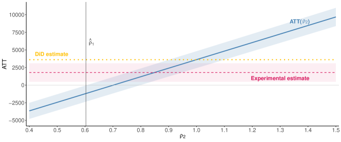
(a) Sensitivity analysis without covariates

(b) Sensitivity analysis with covariates

Notes: Figure 1(a) displays the results from the sensitivity analysis without covariates. Figure 1(b) shows the results from the sensitivity analysis with regression adjustment. The shaded areas depict 95% confidence intervals. Detailed descriptions of the estimators and formulas for the standard errors are given in Appendix A. Data: Sant’Anna and Zhao, 2020b .

The empirical application in this section shows how the selection-based approach to sensitivity analysis can be used to assess the sensitivity of empirical results. A key practical takeaway of our analysis is that because the ATT is a linear function of the selection bias, reducing the selection bias by incorporating baseline covariates is crucial for making empirical results robust to violations of the martingale property necessary for parallel trends under imperfect foresight.

8 Conclusion and implications for practice

In this paper, we study popular parallel trends assumptions through the lens of selection into treatment. We derive necessary and sufficient conditions that clarify the empirical content of parallel trends, suggest selection-based approaches to sensitivity analysis, and provide theory-based templates for justifying parallel trends in applications with and without covariates. Below, we summarize the main implications of our results for practitioners.

Restrictions on selection are unavoidable in DiD designs. Our necessary and sufficient condition in Proposition 3.1 underscores that if researchers are not willing to impose any restrictions on selection, then parallel trends implies that the potential outcomes are constant over time up to deterministic location shifts. Therefore, in realistic settings, relying on parallel trends assumptions implicitly imposes restrictions on the time-varying unobservables and how selection depends on them.

Parallel trends can be compatible with selection on time-varying unobservables. It is well-understood that selection on time-invariant unobservables is compatible with parallel trends in the classical two-way fixed effects model under strict exogeneity (e.g., Blundell and Dias,, 2009). The primitive sufficient conditions in Section 5 provide cases where parallel trends could hold despite selection depending on time-invariant and time-varying unobservables. An important implication is that parallel trends can be compatible with selection on untreated potential outcomes (Example 2.1) and selection on treatment effects (Example 2.2).

Assumptions on selection are useful for sensitivity analyses. Assumptions on selection into treatment are useful for performing sensitivity analysis in applications where the validity of the parallel trends assumption is questionable. To illustrate, we characterize the ATT under imperfect foresight in settings where the martingale assumptions may be violated. For applications where contextual knowledge about selection is available, this characterization is useful for performing sensitivity analysis, computing bounds on the ATT, and developing robust inference procedures.

Contextual knowledge about selection can be used to justify parallel trends. The menu of primitive sufficient conditions in Section 5 provides practitioners with explicit theory-based templates for justifying parallel trends. These conditions consist of different combinations of restrictions on (i) which/how unobservables determine selection and (ii) how their distribution varies over time. We recommend that empirical researchers relying on these conditions use contextual information to assess and explicitly discuss which determinants of the untreated potential outcome affect selection. In doing so, it is crucial to consider the timing of the decision as well as the information set available to the units. Once a suitable selection mechanism is identified, the next step is to discuss the plausibility of the corresponding assumption on the distribution of the unobservables. In this context, periodicity is crucial both to distinguish between time-invariant and time-varying factors and to justify the distributional assumptions.

How to condition on covariates depends on how they enter the outcome model. If the covariates and the unobservable determinants of selection enter the outcome model separably, researchers can condition on the entire time series of covariates and identify the overall ATT. If there are time-varying covariates that interact with the unobservable determinants of selection in the outcome model, researchers should condition on these covariates not changing over time and settle for identification of the ATT for a subpopulation.

Restrictions on nonseparable outcome models can also be used to justify parallel trends. An implication of Section 6.3 is that parallel trends is consistent with a nonseparable outcome model satisfying a combination of time homogeneity and correlated random effects assumptions. This provides researchers with an alternative avenue for justifying parallel trends based on restrictions on the untreated potential outcome and its unobservable determinants.

Appendix (for online publication)

[sections] [sections]l1

Appendix A Implementing sensitivity analyses with covariates

Here we describe how to incorporate covariates into the sensitivity analysis. Using the same arguments as Sections 4 and 6, the martingale property conditional on covariates and in the presence of one additional pre-treatment period is given by

$$E[\ddot{Y}_{i2}(0)|X_{i},\alpha_{i},\varepsilon_{i}^{1}]=\ddot{Y}_{i1}(0)~{}a.s.$$

Conditioning on $X_{i}$ in Proposition 4.1 yields the following characterization of the conditional ATT:

$$\operatorname{ATT}(X_{i})=E[Y_{i2}|G_{i}=1,X_{i}]-E[Y_{i2}|G_{i}=0,X_{i}]-\Delta_{\text{post}}(X_{i}),$$

where

$$\Delta_{\text{post}}(X_{i})\equiv(\rho_{2}-1)\frac{E[G_{i}\dot{Y}_{i1}(0)|X_{i}]}{P(G_{i}=0|X_{i})P(G_{i}=1|X_{i})}+\frac{E[G_{i}\zeta_{i2}|X_{i}]}{P(G_{i}=0|X_{i})P(G_{i}=1|X_{i})},$$

$\rho_{2}\equiv E[\dot{Y}_{i2}(0)^{\perp}\dot{Y}_{i1}(0)^{\perp}]/E[(\dot{Y}_{i1}(0)^{\perp})^{2}]$, $\dot{Y}_{it}(0)^{\perp}=\dot{Y}_{it}(0)-X_{i}^{\prime}E[X_{i}X_{i}^{\prime}]^{-1}E[X_{i}\dot{Y}_{it}(0)]$, and $\zeta_{i2}\equiv E[\dot{Y}_{i2}(0)|X_{i},\alpha_{i},\varepsilon_{i1},\varepsilon_{i0}]-\rho_{2}\dot{Y}_{i1}(0)$.

Now, following Section 4.2 and assuming that $E[G_{i}\zeta_{i2}|X_{i}]=0$ a.s., we have

$$\operatorname{ATT}(X_{i};\rho_{2})=\operatorname{DiD}(X_{i})-(\rho_{2}-1)(E[Y_{i1}|G_{i}=1,X_{i}]-E[Y_{i1}|G_{i}=0,X_{i}]),$$

and, consequently, the unconditional ATT is given by

$$\operatorname{ATT}(\rho_{2})=E[\operatorname{DiD}(X_{i})|G_{i}=1]-(\rho_{2}-1)(E[Y_{i1}|G_{i}=1]-E[E[Y_{i1}|G_{i}=0,X_{i}]|G_{i}=1]).$$ (13)

The term $E[\operatorname{DiD}(X_{i})|G_{i}=1]$ is the DiD estimand under Assumption PT-X (see Section 6). The term $E[Y_{i1}|G_{i}=1]-E[E[Y_{i1}|G_{i}=0,X_{i}]|G_{i}=1]$ measures the selection bias in the pre-treatment period after adjusting for covariate differences.

Because $\operatorname{ATT}(\rho_{2})$ in (13) is the difference between two standard estimands, estimation and inference can proceed based on well-established methods. Here we use a regression-based approach. Alternatively, one could use propensity-score, doubly robust, or double machine learning methods. Specifically, we consider the following estimator,

$$\widehat{\operatorname{ATT}}(\rho_{2})=E_{n}[\widehat{\operatorname{DiD}}(X_{i})|G_{i}=1]-(\rho_{2}-1)(E_{n}[Y_{i1}|G_{i}=1]-E_{n}[\widehat{m}_{10}(X_{i})|G_{i}=1]),$$

where, for a generic $A_{i}$, $E_{n}[A_{i}|G_{i}=1]=\left.\sum_{i=1}^{n}G_{i}A_{i}\right/\sum_{i=1}^{n}G_{i}$ is the sample mean of $A_{i}$ among treated units, $\widehat{m}_{t0}(x)=P(x)^{\prime}\widehat{\theta}_{t0}$ is an estimator of $E[Y_{it}|G_{i}=0,X_{i}=x]$, with $P(x)$ being a known vector of transformations of $x$, and $E_{n}[\widehat{\operatorname{DiD}}(X_{i})|G_{i}=1]$ is the regression-adjusted DiD estimator,

$$E_{n}[\widehat{\operatorname{DiD}}(X_{i})|G_{i}=1]=E_{n}[Y_{i2}-Y_{i1}|G_{i}=1]-E_{n}[\widehat{m}_{\Delta 0}(X_{i})|G_{i}=1],$$

where $\widehat{m}_{\Delta 0}(X_{i})=P(x)^{\prime}\widehat{\theta}_{\Delta 0}$ as an estimator of $E[Y_{i2}-Y_{i1}|G_{i}=0,X_{i}=x]$. In our application, we estimate all regression coefficients using ordinary least squares, and $P(X_{i})$ includes an intercept, linear terms for all covariates (age, years of education, and indicators for high school dropouts, married individuals, Black and Hispanic individuals), age squared, age cubed, and years of schooling squared. This specification is similar to the one in Dehejia and Wahba, (1999, 2002) and Sant’Anna and Zhao, 2020a , except that we omit terms related to lagged outcomes.

Conducting inference here is relatively straightforward as we can leverage results for parametric two-step estimators available in Newey and McFadden, (1994) and Sant’Anna and Zhao, 2020a in a DiD context. More specifically, under mild smoothness and moment conditions, as discussed in Appendix A of Sant’Anna and Zhao, 2020a , we can leverage the delta method to establish the asymptotic linear representation of $\sqrt{n}\left(\widehat{\operatorname{ATT}}(\rho_{2})-{\operatorname{ATT}}(\rho_{2})\right)$ for a given $\rho_{2}$ as

$$\sqrt{n}\left(\widehat{\operatorname{ATT}}(\rho_{2})-{\operatorname{ATT}}(\rho_{2})\right)=\dfrac{1}{\sqrt{n}}\sum_{i=1}^{n}\left(\upsilon^{\text{DiD}}(W_{i},\theta_{0})-(\rho_{2}-1)\upsilon^{\text{bl}}(W_{i},\theta_{0})\right)+o_{p}(1),$$ (14)

where $W_{i}=(Y_{i1},Y_{i2},G_{i},X_{i}^{\prime})^{\prime}$, $\theta_{0}=(\theta_{\Delta 0}^{\prime},\theta_{10}^{\prime})^{\prime}$, and $\upsilon^{\text{DiD}}(W_{i},\theta_{0})$ and $\upsilon^{\text{bl}}(W_{i},\theta_{0})$ are the asymptotic linear representation of $\sqrt{n}\left(E_{n}[\widehat{\operatorname{DiD}}(X_{i})|G_{i}=1]-E[{\operatorname{DiD}}(X_{i})|G_{i}=1]\right)$, and $\sqrt{n}\left((E_{n}[Y_{i1}|G_{i}=1]-E_{n}[\widehat{m}_{10}(X_{i})|G_{i}=1])-(E[Y_{i1}|G_{i}=1]-E[{m}_{10}(X_{i})|G_{i}=1])\right)$, respectively, and are given by

$$\upsilon^{\text{DiD}}(W_{i},\theta_{0}) = \upsilon_{1}^{\text{DiD}}(W_{i},\theta_{0})-\upsilon_{\text{est}}^{\text{DiD}}(W_{i},\theta_{0}),$$

$$\upsilon^{\text{bl}}(W_{i},\theta_{0}) = \upsilon_{1}^{\text{bl}}(W_{i},\theta_{0})-\upsilon_{\text{est}}^{\text{bl}}(W_{i},\theta_{0}),$$

where $\Delta Y_{i}=Y_{i2}-Y_{i1}$,

$$\upsilon^{\text{DiD}}_{1}(W_{i},\theta_{0}) = \dfrac{G_{i}}{E[G_{i}]}\left(\left(\Delta Y_{i}-P(X_{i})^{\prime}\theta_{\Delta 0}\right)-E\left[\Delta Y_{i}-P(X_{i})^{\prime}\theta_{\Delta 0}|G_{i}=1\right]\right),$$

$$\upsilon^{\text{DiD}}_{\text{est}}(W_{i},\theta_{0}) = {E}\left[P(X_{i})^{\prime}|G_{i}=1\right]E\left[P(X_{i})(1-G_{i})P(X_{i})^{\prime}\right]^{-1}(1-G_{i})P(X_{i})(\Delta Y_{i}-P(X_{i})^{\prime}\theta_{\Delta 0}),$$

$$\upsilon^{\text{bl}}_{1}(W_{i},\theta_{0}) = \dfrac{G_{i}}{E[G_{i}]}\left(\left(Y_{1}-P(X_{i})^{\prime}\theta_{10}\right)-E\left[(Y_{i1}-P(X_{i})^{\prime}\theta_{{10}}|G_{i}=1\right]\right),$$

$$\upsilon^{\text{bl}}_{\text{est}}(W_{i},\theta_{0}) = {E}\left[P(X_{i})^{\prime}|G_{i}=1\right]E\left[P(X_{i})(1-G_{i})P(X_{i})^{\prime}\right]^{-1}(1-G_{i})P(X_{i})(Y_{i1}-P(X_{i})^{\prime}\theta_{{10}}).$$

From (14) and the central limit theorem, we have that, for each $\rho_{2}$, as $n\rightarrow\infty$,

$$\sqrt{n}\left(\widehat{\operatorname{ATT}}(\rho_{2})-{\operatorname{ATT}}(\rho_{2})\right)\overset{d}{\rightarrow}N\left(0,E\left[\left(\upsilon^{\text{DiD}}(W_{i},\theta_{0})-(\rho_{2}-1)\upsilon^{\text{bl}}(W_{i},\theta_{0})\right)^{2}\right]\right).$$

The asymptotic variance can be estimated using its sample analog, and one can conduct inference based on it.

Appendix B Disaggregate data and aggregate decisions

In some DiD applications, the data is available at the disaggregate level (e.g., at the individual or firm level), while the decision to select into the treatment is made at the aggregate level (e.g., at the county or state level). The results in the main text directly apply to such settings by interpreting $i$ as indexing the aggregate unit making the selection decision and the unobservables and potential outcomes as aggregate quantities. However, to justify restrictions about selection into treatment, it can be helpful to be more explicit about how selection at the aggregate level is related to the disaggregate level. In the following, we provide a formal framework for doing so. A leading example is when aggregate decisions are based on aggregating preferences at the disaggregate level (e.g., based on voting mechanisms).

Consider a 2$\times$2 DiD setting with $S$ groups, indexed by $s\in\{1,\dots,S\}$. Each group contains $n_{s}$ units, indexed by $i\in\{1,\dots n_{s}\}$. To simplify the exposition, suppose that all groups are the same size, $n_{s}=n$ for $s\in\{1,\dots,S\}$. Following the analysis in the main text, we impose general nonseparable models for the disaggregate potential outcomes,

$$Y_{ist}(0)=\xi_{st}(\alpha_{is},\varepsilon_{ist}).$$

The aggregate potential outcomes are given by

$$Y_{st}(0)=A_{Y(0)}(Y_{1st}(0),\dots,Y_{nst}(0)),$$

where $A_{Y(0)}(\cdot)$ is a potentially nonlinear aggregation function that can depend on $n$. A simple example is when the aggregate outcomes are averages of the disaggregate outcomes, $Y_{st}(0)=n^{-1}\sum_{i=1}^{n}Y_{ist}(0)$.

We consider a sharp DiD setting in which the treatment decisions are made at the group level, so that $G_{s}=G_{is}$ for all $i\in\{1,\dots,n\}$, and researchers rely on parallel trends at the group level,

$$E[Y_{s2}(0)-Y_{s1}(0)|G_{s}=1]=E[Y_{s2}(0)-Y_{s1}(0)|G_{s}=0].$$ (15)

The aggregate selection decision can depend on all unit-level unobservables,

$$G_{s}=g(\alpha_{s},\varepsilon_{s1},\varepsilon_{s2},\nu_{s},\eta_{s1},\eta_{s2}),$$ (16)

where $\alpha_{s}=(\alpha_{1s},\dots,\alpha_{ns})$, $\varepsilon_{s1}=(\varepsilon_{1s1},\dots,\varepsilon_{ns1})$, and $\varepsilon_{s2}=(\varepsilon_{1s2},\dots,\varepsilon_{ns2})$. The vectors $\nu_{s}=(\nu_{1s},\dots,\nu_{ns})$, $\eta_{s1}=(\eta_{1s1},\dots,\eta_{ns1})$, and $\eta_{s2}=(\eta_{1s2},\dots,\eta_{ns2})$ contain additional time-invariant and time-varying unobservables.

All results in the main text directly apply in this setting with $i$ replaced by $s$, such that there are no additional theoretical complications. However, being explicit about the disaggregate level can help “microfound” restrictions on the aggregate selection mechanism $g(\cdot)$, as we illustrate in the following example.

Example B.1 (Simple majority voting).

Suppose that the aggregate selection decision is based on simple majority voting. Each unit submits a vote $V_{is}\in\{0,1\}$, where

$$V_{is}=v(\alpha_{is},\varepsilon_{is1},\varepsilon_{is2},\nu_{is},\eta_{is1},\eta_{is2}).$$ (17)

The voting mechanism (17) accommodates voting based on group-level unobservables and outcomes since the additional unobservables $(\nu_{is},\eta_{is1},\eta_{is2})$ are unrestricted and can contain group-level quantities. Votes can be based on potential outcomes, expected gains, and fixed effects (as in Examples 2.1, 2.2, and 2.3), or other considerations.

The aggregate selection decision under simple majority voting is

$$G_{s}=1\left\{\frac{1}{n}\sum_{i=1}^{n}V_{is}\geq 0.5\right\}.$$ (18)

This selection mechanism is a special case of mechanism (16). Restrictions on the aggregate mechanism (18) can be directly motivated based on assumptions on the units’ voting behavior, their information sets, and discount factors. ∎

Appendix C Necessary and sufficient conditions: extensions

C.1 Parallel trends for any distribution

In the main text, we derive necessary and sufficient conditions for a scenario where researchers are not willing to choose a specific selection mechanism. Here we consider an alternative scenario where researchers are not willing to impose any restrictions on the distribution of unobservables, $F_{\alpha_{i},\varepsilon_{i1},\varepsilon_{i2},\nu_{i},\eta_{i1},\eta_{i2}}$, and require parallel trends to hold for all $F_{\alpha_{i},\varepsilon_{i1},\varepsilon_{i2},\nu_{i},\eta_{i1},\eta_{i2}}$.

The following proposition shows that Assumption PT holds for all $F_{\alpha_{i},\varepsilon_{i1},\varepsilon_{i2},\nu_{i},\eta_{i1},\eta_{i2}}$ in a complete class if and only if selection is independent of the time-invariant and time-varying unobservable determinants of $Y_{it}(0)$. Before we state the proposition, we recall the definition of a complete class of distributions (Equations (4.8)–(4.9) on p.115 in Lehmann and Romano,, 2005).

Definition C.1 (Completeness of a class of distributions).

Let $W$ be a vector of random variables. A family of distributions $\mathcal{F}$ is complete if

$$E[f(W)]=0\quad\text{for all}~{}~{}F_{W}\in\mathcal{F}$$

implies

$$f(w)=0\quad\text{almost everywhere (a.e.)}~{}~{}\mathcal{F}.$$

Proposition C.1 (Necessary and sufficient condition for parallel trends for any distribution of unobservables).

Suppose that $g\in\mathcal{G}_{\text{all}}$ and $F_{\alpha_{i},\varepsilon_{i1},\varepsilon_{i2},\nu_{i},\eta_{i1},\eta_{i2}}\in\mathcal{F}$, where $\mathcal{F}$ is a complete family of probability distributions satisfying $P(g(\alpha_{i},\varepsilon_{i1},\varepsilon_{i2},\nu_{i},\eta_{i1},\eta_{i2})=1)\in(0,1)$ and $P(\dot{Y}_{i1}(0)\neq\dot{Y}_{i2}(0))=1$. Assumption PT holds for all $F_{\alpha_{i},\varepsilon_{i1},\varepsilon_{i2},\nu_{i},\eta_{i1},\eta_{i2}}\in\mathcal{F}$ if and only if $P(G_{i}=1|\alpha_{i},\varepsilon_{i1},\varepsilon_{i2})=P(G_{i}=1)$ a.s. for all $F_{\alpha_{i},\varepsilon_{i1},\varepsilon_{i2},\nu_{i},\eta_{i1},\eta_{i2}}\in\mathcal{F}$.

In Proposition C.1, we require $F_{\alpha_{i},\varepsilon_{i1},\varepsilon_{i2},\nu_{i},\eta_{i1},\eta_{i2}}$ to belong to a complete family of distributions, $\mathcal{F}$. Completeness requires that the class of possible distributions of unobservables is rich enough. This condition is key for showing that parallel trends implies that selection is independent of all unobservable determinants of $Y_{i1}(0)$ and $Y_{i2}(0)$. It holds automatically when $\mathcal{F}$ is unrestricted.

C.2 Multiple periods and multiple groups

Here we generalize our results to DiD designs with multiple periods and multiple groups. The setup and notation are based on Callaway and Sant’Anna, (2021), Sun and Abraham, (2021), and Roth et al., (2023).

Let $t\in\{1,2,\dots,T\}$ index the periods. Suppose that at time $t=1$, no units are treated, at $t=2$, some units become treated, while others remain untreated, and so on. Previously treated units remain treated for all periods. Units can be categorized based on their treatment adoption pattern $D_{i}=(D_{i1},\dots,D_{iT})$. We define the group indicator $G_{i}$ as the first period in which units are treated, $G_{i}=\min\{t\in\{1,\dots,T\}:D_{it}=1\}$, and set $G_{i}=\infty$ for the never-treated units so that $G_{i}\in\{2,\dots,T,\infty\}$.

Potential outcomes are indexed by the entire treatment sequence $(d_{1},\dots,d_{T})\in\{0,1\}^{T}$, $Y_{it}(d_{1},\dots,d_{T})$. Since treatment is an absorbing state, the potential outcomes can be indexed by the first treatment period only. Define $Y_{it}(g)=Y_{it}(\mathbf{0}_{g-1},\mathbf{1}_{T-g+1})$ for $g\in\{2,\dots,T\}$ and $Y_{it}(\infty)=Y_{it}(\mathbf{0}_{T})$, where $\mathbf{0}_{s}\equiv(0,\dots,0)\in\mathbb{R}^{s}$ and $\mathbf{1}_{s}\equiv(1,\dots,1)\in\mathbb{R}^{s}$. Observed outcomes are given by $Y_{it}=\sum_{g\in\{2,\dots,T,\infty\}}1\{G_{i}=g\}Y_{it}(g).$ We maintain a standard no-anticipation assumption (e.g., Roth et al.,, 2023).

Assumption NA.

For $g\in\{2,\dots,T,\infty\}$ and $t<g$, $Y_{it}(g)=Y_{it}(\infty)$.

Our objects of interest are the group-time ATTs,

$$\operatorname{ATT}(g,t)=E[Y_{it}(g)-Y_{it}(\infty)|G_{i}=g].$$ (19)

We impose the following parallel trends assumption to identify the $\operatorname{ATT}(g,t)$.

Assumption PT-MP.

For $(g,t)\in\{2,\dots,T\}^{2}$

$$E[Y_{it}(\infty)-Y_{i(t-1)}(\infty)\,|\,G_{i}=g]=E[Y_{it}(\infty)-Y_{i(t-1)}(\infty)|G_{i}=\infty]$$ (20)

We consider a general nonseparable outcome model,

$$Y_{it}(\infty)=\xi_{t}(\alpha_{i},\varepsilon_{it}),\quad i=1,\dots,n,\quad t=1,\dots,T.$$

Selection into treatment can depend on the unobservable determinants of $Y_{it}(\infty)$ as well as additional unobservables,

$$G_{i}=g(\alpha_{i},\varepsilon_{i1},\dots,\varepsilon_{iT},\nu_{i},\eta_{i1},\dots,\eta_{iT}).$$

As before, let $\mathcal{G}_{\text{all}}$ denote the set of all selection mechanisms $g(\cdot)$ and define the following classes of restricted selection mechanisms, which are natural analogs of those considered in Section 3.

$$\mathcal{G}_{\text{if}} =\{g\in\mathcal{G}_{\text{all}}:g(a,e_{1},\dots,e_{T},v,t_{1},\dots,t_{T})\text{ is a trivial function of $(e_{2},\dots,e_{T},t_{2},\dots,t_{T})$}\}$$

$$\mathcal{G}_{\text{fe}} =\{g\in\mathcal{G}_{\text{all}}:g(a,e_{1},\dots,e_{T},v,t_{1},\dots,t_{T})\text{ is a trivial function of $(e_{1},\dots,e_{T},t_{1},\dots,t_{T})$}\}$$

The following assumption generalizes Assumption SEL to the multiple-period, multiple-group setting. It ensures that the selection mechanisms used to establish the necessary and sufficient conditions for parallel trends are non-degenerate.

Assumption SEL-MP.

There exists a component of $\nu_{i}$, labeled $\nu_{i}^{1}$ (w.l.o.g.), such that $\nu_{i}^{1}\perp\!\!\!\perp(\alpha_{i},\varepsilon_{i1},\dots,\varepsilon_{iT})$. In addition, there exists a non-overlapping partition of the support of $v_{i}^{1}$, $\{B_{g}\}_{g=2}^{T}$, such that $P(v_{i}^{1}\in B_{g})\in(0,1)$ for $g\in\{2,\dots,T\}$.

The following three propositions extend the necessary and sufficient conditions in Propositions 3.1, 3.2, and 3.3 to the more general DiD setting in this section. All these conditions are natural generalizations of their counterparts in the 2$\times$2 case.

Proposition C.2 (Necessary and sufficient condition for $g\in\mathcal{G}_{\text{all}}$).

Suppose that Assumptions NA and SEL-MP hold. Suppose further that either $P(\dot{Y}_{it}(\infty)>\dot{Y}_{i(t-1)}(\infty))<1$ or $P(\dot{Y}_{it}(\infty)<\dot{Y}_{i(t-1)}(\infty))<1$ for each $t\in\{2,\dots,T\}$. Then Assumption PT-MP holds for all $g\in\mathcal{G}_{\text{all}}$ satisfying $P(G_{i}=g)\in(0,1)$ for $g\in\{2,\dots,T,\infty\}$ if and only if $\dot{Y}_{i1}(\infty)=\cdots=\dot{Y}_{iT}(\infty)$ a.s.

Proposition C.3 (Necessary condition for $g\in\mathcal{G}_{\text{if}}$).

Suppose that Assumptions NA and SEL-MP hold. Suppose further that either $P(E[\dot{Y}_{it}(\infty)|\alpha_{i},\varepsilon_{i1}]>E[\dot{Y}_{i(t-1)}(\infty)|\alpha_{i},\varepsilon_{i1}])<1$ or $P(E[\dot{Y}_{it}(\infty)|\alpha_{i},\varepsilon_{i1}]<E[\dot{Y}_{i(t-1)}(\infty)|\alpha_{i},\varepsilon_{i1}])<1$ for each $t\in\{2,\dots,T\}$. If Assumption PT-MP holds for all $g\in\mathcal{G}_{\text{if}}$ satisfying $P(G_{i}=g)\in(0,1)$ for $g\in\{2,\dots,T,\infty\}$, then $E[\dot{Y}_{it}(\infty)|\alpha_{i},\varepsilon_{i1}]=E[\dot{Y}_{i(t-1)}(\infty)|\alpha_{i},\varepsilon_{i1}]$ a.s. for $t\in\{2,\dots,T\}$.

Proposition C.4 (Necessary condition for $g\in\mathcal{G}_{\text{fe}}$).

Suppose that Assumptions NA and SEL-MP hold. Suppose further that either $P(E[\dot{Y}_{it}(\infty)|\alpha_{i}]>E[\dot{Y}_{i(t-1)}(\infty)|\alpha_{i}])<1$ or $P(E[\dot{Y}_{it}(\infty)|\alpha_{i}]<E[\dot{Y}_{i(t-1)}(\infty)|\alpha_{i}])<1$ for each $t\in\{2,\dots,T\}$. If Assumption PT-MP holds for all $g\in\mathcal{G}_{\text{fe}}$ satisfying $P(G_{i}=g)\in(0,1)$ for $g\in\{2,\dots,T,\infty\}$, then $E[\dot{Y}_{it}(\infty)|\alpha_{i}]=E[\dot{Y}_{i(t-1)}(\infty)|\alpha_{i}]$ a.s. for $t\in\{2,\dots,T\}$.

The necessary conditions in Propositions C.3 and C.4 are sufficient for PT-MP under straightforward extensions of the conditions in Section 3.2.

Appendix D Templates for justifying Assumption PT-X

Consider the following separable model with covariates.

Assumption SP-X.

$$Y_{it}(0) =\alpha_{i}+\lambda_{t}+\gamma_{t}(X_{it})+\varepsilon_{it},\quad E[\varepsilon_{it}]=0,\quad i=1,\dots,n,\quad t=1,2.$$ (21)

Assumption SP-X allows for nonparametric covariate-specific trends, which is a key reason for incorporating covariates in DiD analyses. It nests commonly used parametric specifications such as $\gamma_{t}(X_{it})=X_{it}^{\prime}\beta_{t}$. We assume that the treatment does not affect $X_{it}$.

To focus on the different roles played by the time-varying observable and unobservable determinants of $Y_{it}(0)$, we state our sufficient conditions in terms of the projected selection mechanism,

$$\bar{g}(x_{1},x_{2},a,e_{1},e_{2})=E[G_{i}|X_{i1}=x_{1},X_{i2}=x_{2},\alpha_{i}=a,\varepsilon_{i1}=e_{1},\varepsilon_{i2}=e_{2}].$$

Assumption SC1-X.

The following conditions hold:

1. $\bar{g}(x_{1},x_{2},a,e_{1},e_{2})$ is a symmetric function in $e_{1}$ and $e_{2}$.

2. $\varepsilon_{i1},\varepsilon_{i2}|X_{i},\alpha_{i}\overset{d}{=}\varepsilon_{i2},\varepsilon_{i1}|X_{i},\alpha_{i}$.

Assumption SC2-X.

The following conditions hold:

1. $\bar{g}(x_{1},x_{2},a,e_{1},e_{2})$ is a trivial function of $e_{2}$.

2. $E[\varepsilon_{i2}-\varepsilon_{i1}|X_{i},\alpha_{i},\varepsilon_{i1}]=E[\varepsilon_{i2}-\varepsilon_{i1}|X_{i}]$.

Assumption SC3-X.

The following conditions hold:

1. $\bar{g}(x_{1},x_{2},a,e_{1},e_{2})$ is a trivial function of $e_{1}$ and $e_{2}$.

2. $E[\varepsilon_{i1}|X_{i},\alpha_{i}]=E[\varepsilon_{i2}|X_{i},\alpha_{i}]$.

Assumptions SC1-X, SC2-X, and SC3-X are conditional versions of Assumptions SC1, SC2, and SC3. They demonstrate that incorporating time-varying covariates makes the restrictions on the selection mechanism more plausible.

The following proposition shows that Assumptions SC1-X, SC2-X, and SC3-X are sufficient for Assumption PT-X.

Proposition D.1 (Templates for justifying Assumption PT-X).

Suppose that Assumption SP-X holds and $P(G_{i}=1|X_{i})\in(0,1)~{}a.s.$ Then (i) Assumption SC1-X implies Assumption PT-X, (ii) Assumption SC2-X implies Assumption PT-X, and (iii) Assumption SC3-X implies Assumption PT-X.

Proposition D.1 provides theory-based templates for justifying Assumption PT-X in applications based on contextual knowledge about selection into treatment.

Appendix E Proofs of the results in the main text

E.1 Auxiliary lemmas

Lemma E.1.

Let $\omega_{i}$ denote a vector of random variables. Suppose that $P(G_{i}=1|\omega_{i})\in(0,1)$ a.s. Then $E[Y_{i2}(0)-Y_{i1}(0)|G_{i}=1,\omega_{i}]=E[Y_{i2}(0)-Y_{i1}(0)|G_{i}=0,\omega_{i}]$ if and only if $E[G_{i}(Y_{i2}(0)-Y_{i1}(0))|\omega_{i}]=E[G_{i}|\omega_{i}]E[Y_{i2}(0)-Y_{i1}(0)|\omega_{i}]$ a.s.

Proof.

In the following, all equalities involving conditional expectations are understood as a.s. equalities.

“$\Longrightarrow$”: First, note that by the law of total probability, $E[Y_{i2}(0)-Y_{i1}(0)|G_{i}=1,\omega_{i}]=E[Y_{i2}(0)-Y_{i1}(0)|G_{i}=0,\omega_{i}]$ implies

$$E[Y_{i2}(0)-Y_{i1}(0)|G_{i}=1,\omega_{i}]=E[Y_{i2}(0)-Y_{i1}(0)|\omega_{i}].$$

The result follows from noting that $E[Y_{i2}(0)-Y_{i1}(0)|G_{i}=1,\omega_{i}]=\frac{E[G_{i}(Y_{i2}(0)-Y_{i1}(0))|\omega_{i}]}{P(G_{i}=1|\omega_{i})}$ by definition.

“$\Longleftarrow$”: Since $P(G_{i}=1|\omega_{i})\in(0,1)$, it follows that $E[Y_{i2}(0)-Y_{i1}(0)|G_{i}=1,\omega_{i}]=E[Y_{i2}(0)-Y_{i1}(0)|\omega_{i}]$. It then follows that

$$E[Y_{i2}(0)-Y_{i1}(0)|G_{i}=1,\omega_{i}]P(G_{i}=1|\omega_{i})+E[Y_{i2}(0)-Y_{i1}(0)|G_{i}=0,\omega_{i}]P(G_{i}=0|\omega_{i})$$

$$=E[Y_{i2}(0)-Y_{i1}(0)|G_{i}=1,\omega_{i}].$$

The result follows from subtracting the first term on the left-hand side and dividing by $P(G_{i}=0|\omega_{i})$. ∎

Lemma E.2.

For a scalar random variable $W_{i}$, let $\dot{W}_{i}=W_{i}-E[W_{i}]$. If $E[\dot{W}_{i}1\{\dot{W}_{i}\leq 0\}]=0$ or $E[\dot{W}_{i}1\{\dot{W}_{i}\geq 0\}]=0$, then $W_{i}=E[W_{i}]$ a.s.

Proof.

We prove the results for the case where $E[\dot{W}_{i}1\{\dot{W}_{i}\leq 0\}]=0$, since the proof for the other case follows by identical arguments. First, note that by definition $E[\dot{W}_{i}]=0$, which is equivalent to

$$E[\dot{W}_{i}^{+}]=E[\dot{W}_{i}^{-}],$$ (22)

where $\dot{W}_{i}^{+}=|\dot{W}_{i}|1\{\dot{W}_{i}>0\}$ and $\dot{W}_{i}^{-}=|\dot{W}_{i}|1\{\dot{W}_{i}<0\}$.

Now suppose that $E[\dot{W}_{i}1\{\dot{W}_{i}\leq 0\}]=0$ holds, which is equivalent to

$$E[\dot{W}_{i}^{+}1\{\dot{W}_{i}\leq 0\}]=E[\dot{W}_{i}^{-}1\{\dot{W}_{i}\leq 0\}],$$ (23)

since, by definition, $\dot{W}_{i}=\dot{W}_{i}^{+}-\dot{W}_{i}^{-}$. Note that the left-hand side equals zero by the definition of $\dot{W}_{i}^{+}$. As a result, $E[\dot{W}_{i}^{-}1\{\dot{W}_{i}\leq 0\}]=E[\dot{W}_{i}^{-}]=0$. Since $\dot{W}_{i}^{-}\geq 0$, this implies that $P(\dot{W}_{i}^{-}=0)=1$. Now note that $P(\dot{W}_{i}^{-}=0)=P(|\dot{W}_{i}|1\{\dot{W}_{i}<0\}=0)=P(1\{\dot{W}_{i}<0\}=0)=1$, which implies $P(\dot{W}_{i}<0)=0$.

Since $E[\dot{W}_{i}]=0$, (22) further implies that $E[\dot{W}_{i}^{-}]=E[\dot{W}_{i}^{+}]=0$. Since $\dot{W}_{i}^{+}\geq 0$, it follows that $P(\dot{W}_{i}^{+}=0)=1$. Now note that $P(\dot{W}_{i}^{+}=0)=P(|\dot{W}_{i}|1\{\dot{W}_{i}>0\}=0)=P(1\{\dot{W}_{i}>0\}=0)=1$, which implies $P(\dot{W}_{i}>0)=0$.

Together, $P(\dot{W}_{i}<0)=0$ and $P(\dot{W}_{i}>0)=0$ imply that $P(\dot{W}_{i}=0)=1-(P(\dot{W}_{i}<0)+P(\dot{W}_{i}>0))=1$, which completes the proof. ∎

Lemma E.3.

Let $\omega_{i}$ denote a subvector of $(\alpha_{i},\varepsilon_{i1},\varepsilon_{i2})$. Suppose that $P(v_{i}^{1}>c)\in(0,1)$ for some $c\in\mathbb{R}$, and $\nu_{i}^{1}\perp\!\!\!\perp(\alpha_{i},\varepsilon_{i1},\varepsilon_{i2})$.

1. If $P(E[\dot{Y}_{i2}(0)|\omega_{i}]>E[\dot{Y}_{i1}(0)|\omega_{i}])<1$ and Assumption PT holds for $G_{i}=1\{\nu_{i}^{1}>c\}1\{E[\dot{Y}_{i2}(0)-\dot{Y}_{i1}(0)|\omega_{i}]\leq 0\}$, then $E[\dot{Y}_{i2}(0)-\dot{Y}_{i1}(0)|\omega_{i}]=0$ a.s.

2. If $P(E[\dot{Y}_{i2}(0)|\omega_{i}]<E[\dot{Y}_{i1}(0)|\omega_{i}])<1$ and Assumption PT holds for $G_{i}=1\{\nu_{i}^{1}>c\}1\{E[\dot{Y}_{i2}(0)-\dot{Y}_{i1}(0)|\omega_{i}]\geq 0\}$, then $E[\dot{Y}_{i2}(0)-\dot{Y}_{i1}(0)|\omega_{i}]=0$ a.s.

Proof.

We only prove (i). The proof of (ii) follows from the same arguments. Under the maintained assumptions the selection mechanism is nondegenerate,

$$P(1\{\nu_{i}^{1}>c\}1\{E[\dot{Y}_{i2}(0)-\dot{Y}_{i1}(0)|\omega_{i}]\leq 0\}=1)\in(0,1).$$

Thus, by Lemma E.1, Assumption PT holding for $G_{i}=1\{\nu_{i}^{1}>c\}1\{E[\dot{Y}_{i2}(0)-\dot{Y}_{i1}(0)|\omega_{i}]\leq 0\}$ is equivalent to

$$E[1\{\nu_{i}^{1}>c\}1\{E[\dot{Y}_{i2}(0)-\dot{Y}_{i1}(0)|\omega_{i}]\leq 0\}(\dot{Y}_{i2}(0)-\dot{Y}_{i1}(0))]=0,$$

which, by $P(v_{i}^{1}>c)\in(0,1)$ and $\nu_{i}^{1}\perp\!\!\!\perp(\alpha_{i},\varepsilon_{i1},\varepsilon_{i2})$, is equivalent to

$$E[1\{E[\dot{Y}_{i2}(0)-\dot{Y}_{i1}(0)|\omega_{i}]\leq 0\}(\dot{Y}_{i2}(0)-\dot{Y}_{i1}(0))]=0.$$

By the law of iterated expectations (LIE), this is further equivalent to

$$E[1\{E[\dot{Y}_{i2}(0)-\dot{Y}_{i1}(0)|\omega_{i}]\leq 0\}E[\dot{Y}_{i2}(0)-\dot{Y}_{i1}(0)|\omega_{i}]]=0$$

Since $E[E[\dot{Y}_{i2}(0)-\dot{Y}_{i1}(0)|\omega_{i}]]=0$, the result follows by Lemma E.2. ∎

Lemma E.4.

Let $(\alpha_{i},\varepsilon_{i1},\varepsilon_{i2})$ denote a vector of random variables. Suppose that $\varepsilon_{i1},\varepsilon_{i2}|\alpha_{i}\overset{d}{=}\varepsilon_{i2},\varepsilon_{i1}|\alpha_{i}$ holds. Then

1. $F_{\varepsilon_{i1}|\alpha_{i}}(e|a)=F_{\varepsilon_{i2}|\alpha_{i}}(e|a)$ $a.e.$ $(a,e)\in\mathcal{A}\times\mathcal{E}$

2. $F_{\varepsilon_{i1}|\varepsilon_{i2},\alpha_{i}}(e_{1}|e_{2},a)=F_{\varepsilon_{i2}|\varepsilon_{i1},\alpha_{i}}(e_{1}|e_{2},a)$ $a.e.$ $(a,e_{1},e_{2})\in\mathcal{A}\times\mathcal{E}^{2}$.

Proof.

(i) By the definition of the marginal distribution, the conditional exchangeability restriction implies (i) by the following $a.e.$

$$F_{\varepsilon_{i1}|\alpha_{i}}(e_{1}|a) =\lim_{e_{2}\rightarrow\infty}F_{\varepsilon_{i1},\varepsilon_{i2}|\alpha_{i}}(e_{1},e_{2}|a)=\lim_{e_{2}\rightarrow\infty}F_{\varepsilon_{i1},\varepsilon_{i2}|\alpha_{i}}(e_{2},e_{1}|a)=F_{\varepsilon_{i2}|\alpha_{i}}(e_{1}|a).$$ (24)

(ii) By the definition of the conditional distribution and (i) of this lemma, the conditional exchangeability restriction implies (ii) by the following

$$F_{\varepsilon_{i1}|\varepsilon_{i2},\alpha_{i}}(e_{1}|e_{2},a) =\frac{F_{\varepsilon_{i1},\varepsilon_{i2}|\alpha_{i}}(e_{1},e_{2}|a)}{F_{\varepsilon_{i2}|\alpha_{i}}(e_{2}|a)}=\frac{F_{\varepsilon_{i1},\varepsilon_{i2}|\alpha_{i}}(e_{2},e_{1}|a)}{F_{\varepsilon_{i1}|\alpha_{i}}(e_{2}|a)}=F_{\varepsilon_{i2}|\varepsilon_{i1},\alpha_{i}}(e_{1}|e_{2},a),$$ (25)

$a.e.$ $(a,e_{1},e_{2})\in\mathcal{A}\times\mathcal{E}^{2}$. ∎

E.2 Propositions

E.2.1 Proof of Proposition 3.1

“$\Longrightarrow$”: We first consider the case where $P(\dot{Y}_{i2}(0)>\dot{Y}_{i1}(0))<1$. Note that if Assumption PT holds for all $g\in\mathcal{G}_{\text{all}}$, then it holds for $g(\alpha_{i},\varepsilon_{i1},\varepsilon_{i2},\nu_{i},\eta_{i1},\eta_{i2})=1\{\nu_{i}^{1}>c\}1\{\dot{Y}_{i2}(0)-\dot{Y}_{i1}(0)\leq 0\}$. By Assumption SEL and $P(\dot{Y}_{i2}(0)>\dot{Y}_{i1}(0))<1$, we can invoke Lemma E.3.i with $\omega_{i}=(\alpha_{i},\varepsilon_{i1},\varepsilon_{i2})$, which implies $\dot{Y}_{i1}(0)=\dot{Y}_{i2}(0)$ a.s.

The proof for the case where $P(\dot{Y}_{i2}(0)<\dot{Y}_{i1}(0))<1$ follows symmetrically using the selection mechanism $g(\alpha_{i},\varepsilon_{i1},\varepsilon_{i2},\nu_{i},\eta_{i1},\eta_{i2})=1\{\nu_{i}^{1}>c\}1\{\dot{Y}_{i2}(0)-\dot{Y}_{i1}(0)\geq 0\}$ and invoking Lemma E.3.ii.

“$\Longleftarrow$”: This direction is immediate. ∎

E.2.2 Proof of Proposition 3.2

We first consider the case where $P(E[\dot{Y}_{i2}(0)|\alpha_{i},\varepsilon_{i1}]>\dot{Y}_{i1}(0))<1$. Note that if Assumption PT holds for all $g\in\mathcal{G}_{\text{if}}$, then it holds for $g(\alpha_{i},\varepsilon_{i1},\varepsilon_{i2},\nu_{i},\eta_{i1},\eta_{i2})=1\{\nu_{i}^{1}>c\}1\{E[\dot{Y}_{i2}(0)-\dot{Y}_{i1}(0)|\alpha_{i},\varepsilon_{i1}]\leq 0\}$. By Assumption SEL and $P(E[\dot{Y}_{i2}(0)|\alpha_{i},\varepsilon_{i1}]>\dot{Y}_{i1}(0))<1$, we can invoke Lemma E.3.i with $\omega_{i}=(\alpha_{i},\varepsilon_{i1})$, which implies $E[\dot{Y}_{i2}(0)|\alpha_{i},\varepsilon_{i1}]=\dot{Y}_{i1}(0)$ a.s.

The proof for the case where $P(E[\dot{Y}_{i2}(0)|\alpha_{i},\varepsilon_{i1}]<\dot{Y}_{i1}(0))<1$ follows symmetrically using the selection mechanism $g(\alpha_{i},\varepsilon_{i1},\varepsilon_{i2},\nu_{i},\eta_{i1},\eta_{i2})=1\{\nu_{i}^{1}>c\}1\{E[\dot{Y}_{i2}(0)-\dot{Y}_{i1}(0)|\alpha_{i},\varepsilon_{i1}]\geq 0\}$ and invoking Lemma E.3.ii. ∎

E.2.3 Proof of Proposition 3.3

We first consider the case where $P(E[\dot{Y}_{i2}(0)|\alpha_{i}]>E[\dot{Y}_{i1}(0)|\alpha_{i}])<1$. Note that if Assumption PT holds for all $g\in\mathcal{G}_{\text{fe}}$, then it holds for $g(\alpha_{i},\varepsilon_{i1},\varepsilon_{i2},\nu_{i},\eta_{i1},\eta_{i2})=1\{\nu_{i}^{1}>c\}1\{E[\dot{Y}_{i2}(0)-\dot{Y}_{i1}(0)|\alpha_{i}]\leq 0\}$. By Assumption SEL and $P(E[\dot{Y}_{i2}(0)|\alpha_{i}]>E[Y_{i1}(0)|\alpha_{i}])<1$, we can invoke Lemma E.3.i with $\omega_{i}=\alpha_{i}$, which implies $E[\dot{Y}_{i1}(0)|\alpha_{i}]=E[\dot{Y}_{i2}(0)|\alpha_{i}]$ a.s.

The proof for the case where $P(E[\dot{Y}_{i2}(0)|\alpha_{i}]<E[\dot{Y}_{i1}(0)|\alpha_{i}])<1$ follows symmetrically using the selection mechanism $g(\alpha_{i},\varepsilon_{i1},\varepsilon_{i2},\nu_{i},\eta_{i1},\eta_{i2})=1\{\nu_{i}^{1}>c\}1\{E[\dot{Y}_{i2}(0)-\dot{Y}_{i1}(0)|\alpha_{i}]\geq 0\}$ and invoking Lemma E.3.ii. ∎

E.2.4 Proof of Proposition 3.4

(i) Since $g\in\mathcal{G}_{\text{if}}$, then we can simplify the following expression by the LIE as follows,

$$E[G_{i}(\dot{Y}_{i2}(0)-\dot{Y}_{i1}(0))] = E[g(\alpha_{i},\varepsilon_{i1},\nu_{i},\eta_{i1})(\dot{Y}_{i2}(0)-\dot{Y}_{i1}(0))]$$

$$= E[E[E[g(\alpha_{i},\varepsilon_{i1},\nu_{i},\eta_{i1})|\alpha_{i},\varepsilon_{i1},\varepsilon_{i2}](\dot{Y}_{i2}(0)-\dot{Y}_{i1}(0))|\alpha_{i},\varepsilon_{i1}]]$$

$$= E[E[g(\alpha_{i},\varepsilon_{i1},\nu_{i},\eta_{i1})|\alpha_{i},\varepsilon_{i1}]E[\dot{Y}_{i2}(0)-\dot{Y}_{i1}(0)|\alpha_{i},\varepsilon_{i1}]].$$

The third equality follows from $(\nu_{i},\eta_{i1})|\alpha_{i},\varepsilon_{i1},\varepsilon_{i2}\overset{d}{=}(\nu_{i},\eta_{i1})|\alpha_{i},\varepsilon_{i1}$. If $E[\dot{Y}_{i2}(0)|\alpha_{i},\varepsilon_{i1}]=\dot{Y}_{i1}(0)$ a.s., then the last term equals zero, which implies the result by Lemma E.1.

(ii) Similar to (i), since $g\in\mathcal{G}_{\text{fe}}$ and $\nu_{i}|\alpha_{i},\varepsilon_{i1},\varepsilon_{i2}\overset{d}{=}\nu_{i}|\alpha_{i}$, then we can simplify the following expression by the LIE as follows,

$$E[G_{i}(\dot{Y}_{i2}(0)-\dot{Y}_{i1}(0))] = E[g(\alpha_{i},\nu_{i})(\dot{Y}_{i2}(0)-\dot{Y}_{i1}(0))]$$

$$= E[E[E[g(\alpha_{i},\nu_{i})|\alpha_{i},\varepsilon_{i1},\varepsilon_{i2}](\dot{Y}_{i2}(0)-\dot{Y}_{i1}(0))|\alpha_{i}]]$$

$$= E[E[g(\alpha_{i},\nu_{i})|\alpha_{i}]E[\dot{Y}_{i2}(0)-\dot{Y}_{i1}(0)|\alpha_{i}]].$$

If $E[\dot{Y}_{i1}(0)|\alpha_{i}]=E[\dot{Y}_{i2}(0)|\alpha_{i}]$ a.s., then the last term equals zero, which implies the result by Lemma E.1. ∎

E.2.5 Proof of Proposition 4.1

First, we simplify $\Delta_{\text{post}}$ as follows

$$\Delta_{\text{post}} = \frac{E[G_{i}(\dot{Y}_{i2}(0)-\dot{Y}_{i1}(0))]}{P(G_{i}=1)P(G_{i}=0)}$$ (26)

It then follows that

$$\Delta_{\text{post}} = \frac{E[G_{i}(\dot{Y}_{i2}(0)-E[\dot{Y}_{i2}(0)|\alpha_{i},\varepsilon_{i0},\varepsilon_{i1}])]}{P(G_{i}=0)P(G_{i}=1)}$$

$$+\frac{E[E[G_{i}|\alpha_{i},\varepsilon_{i0},\varepsilon_{i1}](E[\dot{Y}_{i2}(0)|\alpha_{i},\varepsilon_{i0},\varepsilon_{i1}]-\dot{Y}_{i1}(0))]}{P(G_{i}=0)P(G_{i}=1)}$$

$$= \frac{E[E[G_{i}|\alpha_{i},\varepsilon_{i0},\varepsilon_{i1}](E[\dot{Y}_{i2}(0)|\alpha_{i},\varepsilon_{i0},\varepsilon_{i1}]-\dot{Y}_{i1}(0))]}{P(G_{i}=0)P(G_{i}=1)}$$

$$= \frac{E[E[G_{i}|\alpha_{i},\varepsilon_{i0},\varepsilon_{i1}](\rho_{2}\dot{Y}_{i1}(0)+\zeta_{i2}-\dot{Y}_{i1}(0))]}{P(G_{i}=0)P(G_{i}=1)}$$

$$= (\rho_{2}-1)\frac{E[G_{i}\dot{Y}_{i1}]}{P(G_{i}=0)P(G_{i}=1)}+\frac{E[G_{i}\zeta_{i2}]}{P(G_{i}=0)P(G_{i}=1)}.$$

The first equality follows by adding and subtracting $E[G_{i}E[\dot{Y}_{i2}(0)|\alpha_{i},\varepsilon_{i0},\varepsilon_{i1}]]$ to the numerator as well as by applying the LIE. The second equality follows from Assumption IF since $E[G_{i}(E[\dot{Y}_{i2}(0)|\alpha_{i},\varepsilon_{i0},\varepsilon_{i1}]-\dot{Y}_{i1}(0))]=0$. The third equality follows by the definition of $\zeta_{i2}\equiv\dot{Y}_{i2}(0)-\rho_{2}\dot{Y}_{i1}(0)$.

∎

E.2.6 Proof of Proposition 5.1

(i) We first show that (i) and (iii) of Assumption SC1 imply the symmetry of $\bar{g}(a,e_{1},e_{2})=E[G_{i}|\alpha_{i}=a,\varepsilon_{i1}=e_{1},\varepsilon_{i2}=e_{2}]$ in $e_{1}$ and $e_{2}$. To do so, we note that these two conditions imply the following for $(a,e_{1},e_{2})\in\mathcal{A}\times\mathcal{E}^{2}$

$$\bar{g}(a,e_{1},e_{2})=\int{{g}(a,e_{1},e_{2},v,t_{1},t_{2})}dF_{\nu_{i},\eta_{i1},\eta_{i2}|\alpha_{i},\varepsilon_{i1},\varepsilon_{i2}}(v,t_{1},t_{2}|a,e_{1},e_{2})$$

$$= \int{g(a,e_{2},e_{1},v,t_{1},t_{2})}dF_{\nu_{i},\eta_{i1},\eta_{i2}|\alpha_{i},\varepsilon_{i1},\varepsilon_{i2}}(v,t_{1},t_{2}|a,e_{2},e_{1})=\bar{g}(a,e_{2},e_{1}),$$ (27)

where the penultimate equality follows by the symmetry of $g(\cdot)$ and $F_{\nu_{i},\eta_{i1},\eta_{i2}|\alpha_{i},\varepsilon_{i1},\varepsilon_{i2}}$ in $e_{1}$ and $e_{2}$ imposed in (i) and (iii) in Assumption SC1, respectively.

Next, by the LIE, we can decompose $E[G_{i}(\varepsilon_{i2}-\varepsilon_{i1})]$ and then invoke the symmetry restrictions on $\bar{g}(\cdot)$ and $F_{\varepsilon_{i1},\varepsilon_{i2}|\alpha_{i}}$ implied by (i) and (iii) of Assumption SC1 as well as (ii) of Assumption SC1, respectively:

$$E[G_{i}(\varepsilon_{i2}-\varepsilon_{i1})]=E[E[\bar{g}(\alpha_{i},\varepsilon_{i1},\varepsilon_{i2})\varepsilon_{i2}|\alpha_{i}]-E[\bar{g}(\alpha_{i},\varepsilon_{i1},\varepsilon_{i2})\varepsilon_{i1}|\alpha_{i}]]$$

$$= \int{\left(\int{\bar{g}(a,e_{1},e_{2})e_{2}}dF_{\varepsilon_{i1},\varepsilon_{i2}|\alpha_{i}}(e_{1},e_{2}|a)-\int{\bar{g}(a,e_{1},e_{2})e_{1}}dF_{\varepsilon_{i1},\varepsilon_{i2}|\alpha_{i}}(e_{1},e_{2}|a)\right)}dF_{\alpha_{i}}(a)$$

$$= \int{\left(\int{\bar{g}(a,e_{2},e_{1})e_{2}}dF_{\varepsilon_{i1},\varepsilon_{i2}|\alpha_{i}}(e_{2},e_{1}|a)-\int{\bar{g}(a,e_{1},e_{2})e_{1}}dF_{\varepsilon_{i1},\varepsilon_{i2}|\alpha_{i}}(e_{1},e_{2}|a)\right)}dF_{\alpha_{i}}(a)=0.$$

The second equality follows from the symmetry restrictions on $\bar{g}(\cdot)$ and $F_{\varepsilon_{i1},\varepsilon_{i2}|\alpha_{i}}$. Together, they imply that both conditional expectations in the parentheses equal $E[\bar{g}(\alpha_{i},\varepsilon_{i1},\varepsilon_{i2})\varepsilon_{i1}|\alpha_{i}]$, and therefore the difference between them is zero. As a result, Assumption SC1 implies Assumption PT.

(ii) This result follows from the proof of Proposition 3.4.i by plugging-in $Y_{it}(0)=\alpha_{i}+\lambda_{t}+\varepsilon_{it}$ for $t=1,2$.

(iii) This result follows from the proof of Proposition 3.4.ii by plugging-in $Y_{it}(0)=\alpha_{i}+\lambda_{t}+\varepsilon_{it}$ for $t=1,2$. ∎

E.2.7 Proof of Proposition 6.1

In this proof, all equalities involving random variables are understood to hold a.s.

First, by Lemma E.1, Assumption PT-NSP under Assumption NSP-X holds if and only if

$$E[G_{i}(Y_{i2}(0)-Y_{i1}(0))|X_{i}^{\lambda},X_{i1}^{\mu}=X_{i2}^{\mu}]$$

$$= E[G_{i}|X_{i}^{\lambda},X_{i1}^{\mu}=X_{i2}^{\mu}]E[Y_{i2}(0)-Y_{i1}(0)|X_{i}^{\lambda},X_{i1}^{\mu}=X_{i2}^{\mu}].$$ (28)

Next, we state some preliminary observations and then proceed to show each statement separately.

Note that, by the LIE, Assumption SEL-CI and the definition of $\bar{g}(\cdot)$, the LHS of (28) equals the following

$$E[G_{i}(Y_{i2}(0)-Y_{i1}(0))|X_{i}^{\lambda},X_{i1}^{\mu}=X_{i2}^{\mu}]$$

$$= E[E[G_{i}|X_{i}^{\mu},X_{i}^{\lambda},\alpha_{i}^{\mu},\alpha_{i}^{\lambda},\varepsilon_{i1}^{\mu},\varepsilon_{i2}^{\mu},\varepsilon_{i1}^{\lambda},\varepsilon_{i2}^{\lambda}](Y_{i2}(0)-Y_{i1}(0))|X_{i}^{\lambda},X_{i1}^{\mu}=X_{i2}^{\mu}]$$

$$= E[\bar{g}(X_{i1}^{\mu},X_{i2}^{\mu},X_{i1}^{\lambda},X_{i2}^{\lambda},\alpha_{i}^{\mu},\varepsilon_{i1}^{\mu},\varepsilon_{i2}^{\mu})(Y_{i2}(0)-Y_{i1}(0))|X_{i}^{\lambda},X_{i1}^{\mu}=X_{i2}^{\mu}].$$ (29)

Similarly, by the LIE, the RHS of (28) equals the following,

$$E[G_{i}|X_{i}^{\lambda},X_{i1}^{\mu}=X_{i2}^{\mu}]E[Y_{i2}(0)-Y_{i1}(0)|X_{i}^{\lambda},X_{i1}^{\mu}=X_{i2}^{\mu}]$$

$$= E[\bar{g}(X_{i1}^{\mu},X_{i2}^{\mu},X_{i1}^{\lambda},X_{i2}^{\lambda},\alpha_{i}^{\mu},\varepsilon_{i1}^{\mu},\varepsilon_{i2}^{\mu})|X_{i}^{\lambda},X_{i1}^{\mu}=X_{i2}^{\mu}]E[Y_{i2}(0)-Y_{i1}(0)|X_{i}^{\lambda},X_{i1}^{\mu}=X_{i2}^{\mu}]$$ (30)

As a result, in the following, to show that Assumptions SC1-NSP, SC2-NSP, and SC3-NSP are sufficient for Assumption PT-NSP, it suffices to show that each assumption implies the following equality,

$$E[\bar{g}(X_{i1}^{\mu},X_{i2}^{\mu},X_{i1}^{\lambda},X_{i2}^{\lambda},\alpha_{i}^{\mu},\varepsilon_{i1}^{\mu},\varepsilon_{i2}^{\mu})(Y_{i2}(0)-Y_{i1}(0))|X_{i}^{\lambda},X_{i1}^{\mu}=X_{i2}^{\mu}]$$

$$= E[\bar{g}(X_{i1}^{\mu},X_{i2}^{\mu},X_{i1}^{\lambda},X_{i2}^{\lambda},\alpha_{i}^{\mu},\varepsilon_{i1}^{\mu},\varepsilon_{i2}^{\mu})|X_{i}^{\lambda},X_{i1}^{\mu}=X_{i2}^{\mu}]E[Y_{i2}(0)-Y_{i1}(0)|X_{i}^{\lambda},X_{i1}^{\mu}=X_{i2}^{\mu}]$$

(i) By Assumption NSP-X, it follows that

$$E[\bar{g}(X_{i1}^{\mu},X_{i2}^{\mu},X_{i1}^{\lambda},X_{i2}^{\lambda},\alpha_{i}^{\mu},\varepsilon_{i1}^{\mu},\varepsilon_{i2}^{\mu})(Y_{i2}(0)-Y_{i1}(0))|X_{i}^{\lambda},X_{i1}^{\mu}=X_{i2}^{\mu}]$$

$$= E[\bar{g}(X_{i1}^{\mu},X_{i2}^{\mu},X_{i1}^{\lambda},X_{i2}^{\lambda},\alpha_{i}^{\mu},\varepsilon_{i1}^{\mu},\varepsilon_{i2}^{\mu})(\mu(X_{i2}^{\mu},\alpha_{i}^{\mu},\varepsilon_{i2}^{\mu})-\mu(X_{i1}^{\mu},\alpha_{i}^{\mu},\varepsilon_{i1}^{\mu}))|X_{i}^{\lambda},X_{i1}^{\mu}=X_{i2}^{\mu}]$$

$$+E[\bar{g}(X_{i1}^{\mu},X_{i2}^{\mu},X_{i1}^{\lambda},X_{i2}^{\lambda},\alpha_{i}^{\mu},\varepsilon_{i1}^{\mu},\varepsilon_{i2}^{\mu})(\lambda_{2}(X_{i2}^{\lambda},\alpha_{i}^{\lambda},\varepsilon_{i2}^{\lambda})-\lambda_{1}(X_{i1}^{\lambda},\alpha_{i}^{\lambda},\varepsilon_{i1}^{\lambda}))|X_{i}^{\lambda},X_{i1}^{\mu}=X_{i2}^{\mu}],$$ (31)

We first examine the first term on the RHS of the above equality. Note that by the symmetry restrictions in Assumptions SC1-NSP.i and SC1-NSP.ii, it follows that a.e. $(a,x^{\mu},x_{1}^{\lambda},x_{2}^{\lambda})\in\mathcal{A}\times\mathcal{X}_{\mu}\times\mathcal{X}_{\lambda}^{2}$

$$E[\bar{g}(X_{i1}^{\mu},X_{i2}^{\mu},X_{i1}^{\lambda},X_{i2}^{\lambda},\alpha_{i}^{\mu},\varepsilon_{i1}^{\mu},\varepsilon_{i2}^{\mu})\mu(X_{i1}^{\mu},\alpha_{i}^{\mu},\varepsilon_{i1}^{\mu})|X_{i}^{\lambda}=(x_{1}^{\lambda},x_{2}^{\lambda}),X_{i1}^{\mu}=X_{i2}^{\mu}=x^{\mu},\alpha_{i}^{\mu}=a]$$

$$= \int{\bar{g}(x^{\mu},x^{\mu},x_{1}^{\lambda},x_{2}^{\lambda},a,e_{1},e_{2})\mu(x^{\mu},a,e_{1})}dF_{\varepsilon_{i1}^{\mu},\varepsilon_{i2}^{\mu}|X_{i}^{\lambda},X_{i1}^{\mu}=X_{i2}^{\mu},\alpha_{i}^{\mu}}(e_{1},e_{2}|(x_{1}^{\lambda},x_{2}^{\lambda}),x^{\mu},a)$$

$$= \int{\bar{g}(x^{\mu},x^{\mu},x_{1}^{\lambda},x_{2}^{\lambda},a,e_{2},e_{1})\mu(x^{\mu},a,e_{1})}dF_{\varepsilon_{i1}^{\mu},\varepsilon_{i2}^{\mu}|X_{i}^{\lambda},X_{i1}^{\mu}=X_{i2}^{\mu},\alpha_{i}^{\mu}}(e_{2},e_{1}|(x_{1}^{\lambda},x_{2}^{\lambda}),x^{\mu},a)$$

$$= E[\bar{g}(X_{i1}^{\mu},X_{i2}^{\mu},X_{i1}^{\lambda},X_{i2}^{\lambda},\alpha_{i}^{\mu},\varepsilon_{i1}^{\mu},\varepsilon_{i2}^{\mu})\mu(X_{i2}^{\mu},\alpha_{i}^{\mu},\varepsilon_{i2}^{\mu})|X_{i}^{\lambda}=(x_{1}^{\lambda},x_{2}^{\lambda}),X_{i1}^{\mu}=X_{i2}^{\mu}=x^{\mu},\alpha_{i}^{\mu}=a].$$ (32)

As a result, the first summand in (31) equals zero by (32) and the LIE.

Next, we consider the second summand in (31),

$$E[\bar{g}(X_{i1}^{\mu},X_{i2}^{\mu},X_{i1}^{\lambda},X_{i2}^{\lambda},\alpha_{i}^{\mu},\varepsilon_{i1}^{\mu},\varepsilon_{i2}^{\mu})(\lambda_{2}(X_{i2}^{\lambda},\alpha_{i}^{\lambda},\varepsilon_{i2}^{\lambda})-\lambda_{1}(X_{i1}^{\lambda},\alpha_{i}^{\lambda},\varepsilon_{i1}^{\lambda}))|X_{i}^{\lambda},X_{i1}^{\mu}=X_{i2}^{\mu}]$$

$$= E[\bar{g}(X_{i1}^{\mu},X_{i2}^{\mu},X_{i1}^{\lambda},X_{i2}^{\lambda},\alpha_{i}^{\mu},\varepsilon_{i1}^{\mu},\varepsilon_{i2}^{\mu})|X_{i}^{\lambda},X_{i1}^{\mu}=X_{i2}^{\mu}]E[\lambda_{2}(X_{i2}^{\lambda},\alpha_{i}^{\lambda},\varepsilon_{i2}^{\lambda})-\lambda_{1}(X_{i1}^{\lambda},\alpha_{i}^{\lambda},\varepsilon_{i1}^{\lambda})|X_{i}^{\lambda},X_{i1}^{\mu}=X_{i2}^{\mu}]$$

$$= E[\bar{g}(X_{i1}^{\mu},X_{i2}^{\mu},X_{i1}^{\lambda},X_{i2}^{\lambda},\alpha_{i}^{\mu},\varepsilon_{i1}^{\mu},\varepsilon_{i2}^{\mu})|X_{i}^{\lambda},X_{i1}^{\mu}=X_{i2}^{\mu}]E[Y_{i2}(0)-Y_{i1}(0)|X_{i}^{\lambda},X_{i1}^{\mu}=X_{i2}^{\mu}].$$ (33)

The first equality follows from the conditional independence assumption in Assumption SC1-NSP.iii. The last equality follows from the time homogeneity of $F_{\varepsilon_{it}^{\mu}|X_{i}^{\mu},X_{i}^{\lambda},\alpha_{i}^{\mu}}$, which follows from the exchangeability restriction in Assumption SC1-NSP.ii by Lemma E.4, and implies that $E[\mu(X_{i2}^{\mu},\alpha_{i}^{\mu},\varepsilon_{i2}^{\mu})-\mu(X_{i1}^{\mu},\alpha_{i}^{\mu},\varepsilon_{i1}^{\mu})|X_{i}^{\lambda},X_{i1}^{\mu}=X_{i2}^{\mu},\alpha_{i}^{\mu}]=0$ and

$$E[Y_{i2}(0)-Y_{i1}(0)|X_{i}^{\lambda},X_{i1}^{\mu}=X_{i2}^{\mu}]=E[\lambda_{2}(X_{i2}^{\lambda},\alpha_{i}^{\lambda},\varepsilon_{i2}^{\lambda})-\lambda_{1}(X_{i1}^{\lambda},\alpha_{i}^{\lambda},\varepsilon_{i1}^{\lambda}))|X_{i}^{\lambda},X_{i1}^{\mu}=X_{i2}^{\mu}]$$

by the LIE. As a result, the above implies that Assumption PT-NSP holds.

(ii) By Assumption SC2-NSP.i, we can define $\check{\bar{g}}(x_{1}^{\mu},x_{2}^{\mu},x_{1}^{\lambda},x_{2}^{\lambda},a^{\mu},e_{1}^{\lambda})=\bar{g}(x_{1}^{\mu},x_{2}^{\mu},x_{1}^{\lambda},x_{2}^{\lambda},a^{\mu},e_{1}^{\lambda},e_{2}^{\lambda}).$ By Assumption NSP-X, it follows that

$$E[\check{\bar{g}}(X_{i1}^{\mu},X_{i2}^{\mu},X_{i1}^{\lambda},X_{i2}^{\lambda},\alpha_{i}^{\mu},\varepsilon_{i1}^{\mu})(Y_{i2}(0)-Y_{i1}(0))|X_{i}^{\lambda},X_{i1}^{\mu}=X_{i2}^{\mu}]$$

$$= E[\check{\bar{g}}(X_{i1}^{\mu},X_{i2}^{\mu},X_{i1}^{\lambda},X_{i2}^{\lambda},\alpha_{i}^{\mu},\varepsilon_{i1}^{\mu})\Delta_{\mu,i}|X_{i}^{\lambda},X_{i1}^{\mu}=X_{i2}^{\mu}]$$

$$+E[\check{\bar{g}}(X_{i1}^{\mu},X_{i2}^{\mu},X_{i1}^{\lambda},X_{i2}^{\lambda},\alpha_{i}^{\mu},\varepsilon_{i1}^{\mu})(\lambda_{2}(X_{i2}^{\lambda},\alpha_{i}^{\lambda},\varepsilon_{i2}^{\lambda})-\lambda_{1}(X_{i1}^{\lambda},\alpha_{i}^{\lambda},\varepsilon_{i1}^{\lambda}))|X_{i}^{\lambda},X_{i1}^{\mu}=X_{i2}^{\mu}]$$

$$= E[\check{\bar{g}}(X_{i1}^{\mu},X_{i2}^{\mu},X_{i1}^{\lambda},X_{i2}^{\lambda},\alpha_{i}^{\mu},\varepsilon_{i1}^{\mu})|X_{i}^{\lambda},X_{i1}^{\mu}=X_{i2}^{\mu}]E[\Delta_{\mu,i}|X_{i}^{\lambda},X_{i1}^{\mu}=X_{i2}^{\mu}]$$

$$+E[\check{\bar{g}}(X_{i1}^{\mu},X_{i2}^{\mu},X_{i1}^{\lambda},X_{i2}^{\lambda},\alpha_{i}^{\mu},\varepsilon_{i1}^{\mu})|X_{i}^{\lambda},X_{i1}^{\mu}=X_{i2}^{\mu}]E[\lambda_{2}(X_{i2}^{\lambda},\alpha_{i}^{\lambda},\varepsilon_{i2}^{\lambda})-\lambda_{1}(X_{i1}^{\lambda},\alpha_{i}^{\lambda},\varepsilon_{i1}^{\lambda})|X_{i}^{\lambda},X_{i1}^{\mu}=X_{i2}^{\mu}]$$

$$= E[\check{\bar{g}}(X_{i1}^{\mu},X_{i2}^{\mu},X_{i1}^{\lambda},X_{i2}^{\lambda},\alpha_{i}^{\mu},\varepsilon_{i1}^{\mu})|X_{i}^{\lambda},X_{i1}^{\mu}=X_{i2}^{\mu}]E[Y_{i2}(0)-Y_{i1}(0)|X_{i}^{\lambda},X_{i1}^{\mu}=X_{i2}^{\mu}]$$ (34)

The second equality follows from the conditional independence conditions in Assumptions SC2-NSP.ii and SC2-NSP.iii. The last equality follows from Assumption NSP-X. Equation (34) then implies Assumption PT-NSP.

(iii) By Assumption SC3-NSP.i, we can define $\check{\bar{g}}(x_{1}^{\mu},x_{2}^{\mu},x_{1}^{\lambda},x_{2}^{\lambda},a^{\mu})=\bar{g}(x_{1}^{\mu},x_{2}^{\mu},x_{1}^{\lambda},x_{2}^{\lambda},a^{\mu},e_{1}^{\lambda},e_{2}^{\lambda}).$ Now by the Assumption NSP-X and SC3-NSP.i, it follows that

$$E[\check{\bar{g}}(X_{i1}^{\mu},X_{i2}^{\mu},X_{i1}^{\lambda},X_{i2}^{\lambda},\alpha_{i}^{\mu})(Y_{i2}(0)-Y_{i1}(0))|X_{i}^{\lambda},X_{i1}^{\mu}=X_{i2}^{\mu}]$$

$$= E[\check{\bar{g}}(X_{i1}^{\mu},X_{i2}^{\mu},X_{i1}^{\lambda},X_{i2}^{\lambda},\alpha_{i}^{\mu})(\mu(X_{i2}^{\mu},\alpha_{i}^{\mu},\varepsilon_{i2}^{\mu})-\mu(X_{i1}^{\mu},\alpha_{i}^{\mu},\varepsilon_{i1}^{\mu}))|X_{i}^{\lambda},X_{i1}^{\mu}=X_{i2}^{\mu}]$$

$$+E[\check{\bar{g}}(X_{i1}^{\mu},X_{i2}^{\mu},X_{i1}^{\lambda},X_{i2}^{\lambda},\alpha_{i}^{\mu})(\lambda_{2}(X_{i2}^{\lambda},\alpha_{i}^{\lambda},\varepsilon_{i2}^{\lambda})-\lambda_{1}(X_{i1}^{\lambda},\alpha_{i}^{\lambda},\varepsilon_{i1}^{\lambda}))|X_{i}^{\lambda},X_{i1}^{\mu}=X_{i2}^{\mu}]$$

$$= E[\check{\bar{g}}(X_{i1}^{\mu},X_{i2}^{\mu},X_{i1}^{\lambda},X_{i2}^{\lambda},\alpha_{i}^{\mu})E[\mu(X_{i2}^{\mu},\alpha_{i}^{\mu},\varepsilon_{i2}^{\mu})-\mu(X_{i1}^{\mu},\alpha_{i}^{\mu},\varepsilon_{i1}^{\mu})|X_{i}^{\lambda},X_{i1}^{\mu}=X_{i2}^{\mu},\alpha_{i}^{\mu}]|X_{i}^{\lambda},X_{i1}^{\mu}=X_{i2}^{\mu}]$$

$$+E[\check{\bar{g}}(X_{i1}^{\mu},X_{i2}^{\mu},X_{i1}^{\lambda},X_{i2}^{\lambda},\alpha_{i}^{\mu})|X_{i}^{\lambda},X_{i1}^{\mu}=X_{i2}^{\mu}]E[\lambda_{2}(X_{i2}^{\lambda},\alpha_{i}^{\lambda},\varepsilon_{i2}^{\lambda})-\lambda_{1}(X_{i1}^{\lambda},\alpha_{i}^{\lambda},\varepsilon_{i1}^{\lambda})|X_{i}^{\lambda},X_{i1}^{\mu}=X_{i2}^{\mu}]$$

$$= E[\check{\bar{g}}(X_{i1}^{\mu},X_{i2}^{\mu},X_{i1}^{\lambda},X_{i2}^{\lambda},\alpha_{i}^{\mu})|X_{i}^{\lambda},X_{i1}^{\mu}=X_{i2}^{\mu}]E[\lambda_{2}(X_{i2}^{\lambda},\alpha_{i}^{\lambda},\varepsilon_{i2}^{\lambda})-\lambda_{1}(X_{i1}^{\lambda},\alpha_{i}^{\lambda},\varepsilon_{i1}^{\lambda})|X_{i}^{\lambda},X_{i1}^{\mu}=X_{i2}^{\mu}]$$

$$= E[\check{\bar{g}}(X_{i1}^{\mu},X_{i2}^{\mu},X_{i1}^{\lambda},X_{i2}^{\lambda},\alpha_{i}^{\mu})|X_{i}^{\lambda},X_{i1}^{\mu}=X_{i2}^{\mu}]E[Y_{i2}(0)-Y_{i1}(0)|X_{i}^{\lambda},X_{i1}^{\mu}=X_{i2}^{\mu}],$$

where the first equality follows from Assumption NSP-X. The second equality follows by applying the LIE to the first term and the conditional independence imposed in Assumption SC3-NSP.iii to the second term. The first term on the RHS of the second equality equals zero by the conditioning on $X_{i1}^{\mu}=X_{i2}^{\mu}$ and the time homogeneity condition in Assumption SC3-NSP.ii. The last equality follows from noting, similar as in the proof of (i), that since $E[\mu(X_{i2}^{\mu},\alpha_{i}^{\mu},\varepsilon_{i2}^{\mu})-\mu(X_{i1}^{\mu},\alpha_{i}^{\mu},\varepsilon_{i1}^{\mu})|X_{i}^{\lambda},X_{i1}^{\mu}=X_{i2}^{\mu},\alpha_{i}^{\mu}]=0$,

$$E[Y_{i2}(0)-Y_{i1}(0)|X_{i}^{\lambda},X_{i1}^{\mu}=X_{i2}^{\mu}]=E[\lambda_{2}(X_{i2}^{\lambda},\alpha_{i}^{\lambda},\varepsilon_{i2}^{\lambda})-\lambda_{1}(X_{i1}^{\lambda},\alpha_{i}^{\lambda},\varepsilon_{i1}^{\lambda})|X_{i}^{\lambda},X_{i1}^{\mu}=X_{i2}^{\mu}]$$

by the LIE. This completes the proof. ∎

E.2.8 Proof of Proposition 6.2

Under Assumption NSP-X,

$$E[Y_{i2}(0)-Y_{i1}(0)|G_{i},X_{i}^{\lambda},X_{i1}^{\mu}=X_{i2}^{\mu}]$$

$$= E[\mu(X_{i2}^{\mu},\alpha_{i}^{\mu},\varepsilon_{i2}^{\mu})-\mu(X_{i1}^{\mu},\alpha_{i}^{\mu},\varepsilon_{i1}^{\mu})|G_{i},X_{i}^{\lambda},X_{i1}^{\mu}=X_{i2}^{\mu}]$$ (35)

$$+E[\lambda_{2}(X_{i2}^{\lambda},\alpha_{i}^{\lambda},\varepsilon_{i2}^{\lambda})-\lambda_{1}(X_{i1}^{\lambda},\alpha_{i}^{\lambda},\varepsilon_{i1}^{\lambda})|G_{i},X_{i}^{\lambda},X_{i1}^{\mu}=X_{i2}^{\mu}].$$ (36)

The remainder of the proof follows in two steps. First, we show that the term in (35) equals zero under our assumptions. Second, we show that the second term is conditionally mean independent of $G_{i}$, which implies Assumption PT-NSP.

We proceed to show that under Assumption TH the term in (35) equals zero by the following,

$$E[\mu(X_{i1}^{\mu},\alpha_{i}^{\mu},\varepsilon_{i1}^{\mu})|G_{i}=g,X_{i}^{\lambda}=(x_{1}^{\lambda},x_{2}^{\lambda}),X_{i1}^{\mu}=X_{i2}^{\mu}=x^{\mu}]$$

$$= \int{\mu(x^{\mu},a^{\mu},e^{\mu})}dF_{\alpha_{i}^{\mu},\varepsilon_{i1}^{\mu}|G_{i},X_{i}^{\mu},X_{i}^{\lambda}}(a^{\mu},e^{\mu}|g,(x^{\mu},x^{\mu}),(x_{1}^{\lambda},x_{2}^{\lambda}))$$

$$= \int{\mu(x^{\mu},a^{\mu},e^{\mu})}dF_{\alpha_{i}^{\mu},\varepsilon_{i2}^{\mu}|G_{i},X_{i}^{\mu},X_{i}^{\lambda}}(a^{\mu},e^{\mu}|g,(x^{\mu},x^{\mu}),(x_{1}^{\lambda},x_{2}^{\lambda}))$$

$$= E[\mu(X_{i2}^{\mu},\alpha_{i}^{\mu},\varepsilon_{i2}^{\mu})|G_{i}=g,X_{i}^{\lambda}=(x_{1}^{\lambda},x_{2}^{\lambda}),X_{i1}^{\mu}=X_{i2}^{\mu}=x^{\mu}],$$ (37)

where the first and last equalities follow by definition, whereas the penultimate equality follows from Assumption TH noting that it implies $\alpha_{i}^{\mu},\varepsilon_{i1}^{\mu}|G_{i},X_{i}^{\mu},X_{i}^{\lambda}\overset{d}{=}\alpha_{i}^{\mu},\varepsilon_{i2}^{\mu}|G_{i},X_{i}^{\mu},X_{i}^{\lambda}$.

Finally, we show that Assumption CRE implies the following for (36)

$$E[\lambda_{2}(X_{i2}^{\lambda},\alpha_{i}^{\lambda},\varepsilon_{i2}^{\lambda})-\lambda_{1}(X_{i1}^{\lambda},\alpha_{i}^{\lambda},\varepsilon_{i1}^{\lambda})|G_{i}=g,X_{i}^{\lambda}=(x_{1}^{\lambda},x_{2}^{\lambda}),X_{i1}^{\mu}=X_{i2}^{\mu}=x^{\mu}]$$

$$= \int{(\lambda_{2}(x_{2}^{\lambda},a^{\lambda},e_{2}^{\lambda})-\lambda_{1}(x_{1}^{\lambda},a^{\lambda},e_{1}^{\lambda}))}dF_{\alpha_{i}^{\lambda},\varepsilon_{i1}^{\lambda},\varepsilon_{i2}^{\lambda}|G_{i},X_{i}^{\mu},X_{i}^{\lambda}}(a^{\lambda},e_{1}^{\lambda},e_{2}^{\lambda}|g,(x^{\mu},x^{\mu}),(x_{1}^{\lambda},x_{2}^{\lambda}))$$

$$= \int{(\lambda_{2}(x_{2}^{\lambda},a^{\lambda},e_{2}^{\lambda})-\lambda_{1}(x_{1}^{\lambda},a^{\lambda},e_{1}^{\lambda}))}dF_{\alpha_{i}^{\lambda},\varepsilon_{i1}^{\lambda},\varepsilon_{i2}^{\lambda}|X_{i}^{\mu},X_{i}^{\lambda}}(a^{\lambda},e_{1}^{\lambda},e_{2}^{\lambda}|(x^{\mu},x^{\mu}),(x_{1}^{\lambda},x_{2}^{\lambda}))$$

$$= E[\lambda_{2}(X_{i2}^{\lambda},\alpha_{i}^{\lambda},\varepsilon_{i2}^{\lambda})-\lambda_{1}(X_{i1}^{\lambda},\alpha_{i}^{\lambda},\varepsilon_{i1}^{\lambda})|X_{i}^{\lambda}=(x_{1}^{\lambda},x_{2}^{\lambda}),X_{i1}^{\mu}=X_{i2}^{\mu}=x^{\mu}],$$ (38)

where the penultimate equality follows by Assumption CRE. This completes the proof. ∎

E.2.9 Proof of Proposition 6.3

Throughout this proof, equalities involving conditioning statements are understood to hold $a.e.$ We proceed to show each result separately.

(i) It suffices to show (i.a) Assumptions SC1-NSP.i and SC1-NSP.ii imply Assumption TH and (i.b) Assumptions SC1-NSP.i and SC1-NSP.iii imply Assumption CRE.

(i.a) Consider

$$F_{\varepsilon_{i1}^{\mu},G_{i}|X_{i}^{\mu},X_{i}^{\lambda},\alpha_{i}^{\mu}}(e_{1},g|x^{\mu},x^{\lambda},a)=F_{G_{i}|\varepsilon_{i1}^{\mu},X_{i}^{\mu},X_{i}^{\lambda},\alpha_{i}^{\mu}}(g|e_{1},x^{\mu},x^{\lambda},a)F_{\varepsilon_{i1}^{\mu}|X_{i}^{\mu},X_{i}^{\lambda},\alpha_{i}^{\mu}}(e_{1}|x^{\mu},x^{\mu},a),$$

where $x^{\mu}=(x_{1}^{\mu},x_{2}^{\mu})$ and $x^{\lambda}=(x_{1}^{\lambda},x_{2}^{\lambda})$. Assumption SC1-NSP.ii implies $F_{\varepsilon_{i1}^{\mu}|X_{i}^{\mu},X_{i}^{\lambda},\alpha_{i}^{\mu}}(e|x^{\mu},x^{\lambda},a)=F_{\varepsilon_{i2}^{\mu}|X_{i}^{\mu},X_{i}^{\lambda},\alpha_{i}^{\mu}}(e|x^{\mu},x^{\lambda},a)$ as well as $F_{\varepsilon_{i1}^{\mu}|\varepsilon_{i2}^{\mu},X_{i}^{\mu},X_{i}^{\lambda},\alpha_{i}^{\mu}}(e_{1}|e_{2},x^{\mu},x^{\lambda},a)=F_{\varepsilon_{i2}^{\mu}|\varepsilon_{i1}^{\mu},X_{i}^{\mu},X_{i}^{\lambda},\alpha_{i}^{\mu}}(e_{1}|e_{2},x^{\mu},x^{\lambda},a)$ by Lemma E.4, which implies

$$F_{G_{i}|\varepsilon_{i1}^{\mu},X_{i}^{\mu},X_{i}^{\lambda},\alpha_{i}^{\mu}}(g|e_{1},x^{\mu},x^{\lambda},a)$$

$$= \int{1\{g(x_{1}^{\mu},x_{2}^{\mu},x_{1}^{\lambda},x_{2}^{\lambda},a,e_{1},e_{2})\leq g\}}dF_{\varepsilon_{i2}^{\mu}|\varepsilon_{i1}^{\mu},X_{i}^{\mu},X_{i}^{\lambda},\alpha_{i}^{\mu}}(e_{2}|e_{1},x^{\mu},x^{\lambda},a)$$

$$= \int{1\{g(x_{1}^{\mu},x_{2}^{\mu},x_{1}^{\lambda},x_{2}^{\lambda},a,e_{2},e_{1})\leq g\}}dF_{\varepsilon_{i1}^{\mu}|\varepsilon_{i2}^{\mu},X_{i}^{\mu},X_{i}^{\lambda},\alpha_{i}^{\mu}}(e_{2}|e_{1},x^{\mu},x^{\lambda},a)$$

$$= F_{G_{i}|\varepsilon_{i2}^{\mu},X_{i}^{\mu},X_{i}^{\lambda},\alpha_{i}^{\mu}}(g|e_{1},x^{\mu},x^{\lambda},a).$$ (39)

As a result,

$$F_{\varepsilon_{i1}^{\mu},G_{i}|X_{i}^{\mu},X_{i}^{\lambda},\alpha_{i}^{\mu}}(e_{1},g|x^{\mu},x^{\lambda},a)=F_{G_{i}|\varepsilon_{i1}^{\mu},X_{i}^{\mu},X_{i}^{\lambda},\alpha_{i}^{\mu}}(g|e_{1},x^{\mu},x^{\lambda},a)F_{\varepsilon_{i1}^{\mu}|X_{i}^{\mu},X_{i}^{\lambda},\alpha_{i}^{\mu}}(e_{1}|x^{\mu},x^{\lambda},a)$$

$$= F_{G_{i}|\varepsilon_{i2}^{\mu},X_{i}^{\mu},X_{i}^{\lambda},\alpha_{i}^{\mu}}(g|e_{1},x^{\mu},x^{\lambda},a)F_{\varepsilon_{i2}^{\mu}|X_{i}^{\mu},X_{i}^{\lambda},\alpha_{i}^{\mu}}(e_{1}|x^{\mu},x^{\lambda},a)$$

$$= F_{\varepsilon_{i2}^{\mu},G_{i}|X_{i}^{\mu},X_{i}^{\lambda},\alpha_{i}^{\mu}}(e_{1},g|x^{\mu},x^{\lambda},a).$$ (40)

This implies Assumption TH by the definition of a conditional distribution,

$$F_{\varepsilon_{it}^{\mu}|G_{i},X_{i}^{\mu},X_{i}^{\lambda},\alpha_{i}^{\mu}}(e|g,x^{\mu},x^{\lambda},a)=\frac{F_{\varepsilon_{it}^{\mu},G_{i}|X_{i}^{\mu},X_{i}^{\lambda}\alpha_{i}^{\mu}}(e,g|x^{\mu},x^{\lambda})}{F_{G_{i}|X_{i}^{\mu},X_{i}^{\lambda}\alpha_{i}^{\mu}}(g|x^{\mu},x^{\lambda},a)},$$

where $F_{G_{i}|X_{i}^{\mu},X_{i}^{\lambda},\alpha_{i}^{\mu}}(g|x^{\mu},x^{\lambda},a)>0$ a.s. for $g=0,1$ by assumption.

(i.b) This statement follows in a straightforward manner from the definition of $G_{i}$ in Assumption SC1-NSP.i and the conditional independence condition in Assumption SC1-NSP.iii which together imply Assumption CRE. This completes the proof of (i).

(ii) To show the result, it suffices to show that (ii.a) Assumptions SC3-NSP.i and SC3-NSP.ii imply Assumption TH and (ii.b) Assumptions SC3-NSP.i and SC3-NSP.iii imply Assumption CRE.

(ii.a) Under Assumptions SC3-NSP.i and SC3-NSP.ii, $G_{i}=g(X_{i1}^{\mu},X_{i2}^{\mu},X_{i1}^{\lambda},X_{i2}^{\lambda},\alpha_{i}^{\mu})$ is a degenerate random variable equaling either zero or one with probability one conditional on $X_{i}^{\mu}$, $X_{i}^{\lambda}$ and $\alpha_{i}^{\mu}$. As a result,

$$F_{\varepsilon_{it}^{\mu}|G_{i},X_{i}^{\mu},X_{i}^{\lambda},\alpha_{i}^{\mu}}(e|g,x^{\mu},x^{\lambda},a)$$

$$= \sum_{g=0,1}P(\varepsilon_{it}^{\mu}\leq e|G_{i}=g(x_{1}^{\mu},x_{2}^{\mu},x_{1}^{\lambda},x_{2}^{\lambda},a),X_{i}^{\mu}=x^{\mu},X_{i}^{\lambda}=x^{\lambda},\alpha_{i}^{\mu}=a)1\{g(x_{1}^{\mu},x_{2}^{\mu},x_{1}^{\lambda},x_{2}^{\lambda},a)=g\}$$

$$= \sum_{g=0,1}P(\varepsilon_{it}^{\mu}\leq e|X_{i}^{\mu}=x^{\mu},X_{i}^{\lambda}=x^{\lambda},\alpha_{i}^{\mu}=a)1\{g(x_{1}^{\mu},x_{2}^{\mu},x_{1}^{\lambda},x_{2}^{\lambda},a)=g\}$$

$$= \sum_{g=0,1}F_{\varepsilon_{it}^{\mu}|X_{i}^{\mu},X_{i}^{\lambda},\alpha_{i}^{\mu}}(e|a,x^{\mu},x^{\lambda})1\{g(x_{1}^{\mu},x_{2}^{\mu},x_{1}^{\lambda},x_{2}^{\lambda},a)=g\}.$$ (41)

As a result, Assumption SC3-NSP.i together with the time homogeneity of $F_{\varepsilon_{it}^{\mu}|X_{i}^{\mu},X_{i}^{\lambda},\alpha_{i}^{\mu}}$ in Assumption SC3-NSP.ii is sufficient for the time homogeneity of $F_{\varepsilon_{it}^{\mu}|G_{i},X_{i}^{\mu},X_{i}^{\lambda},\alpha_{i}^{\mu}}$, which yields Assumption TH.

(ii.b) The statement (ii.b) is immediate from noting that Assumption SC3-NSP.iii together with $G_{i}=g(X_{i1}^{\mu},X_{i2}^{\mu},X_{i1}^{\lambda},X_{i2}^{\lambda},\alpha_{i}^{\mu})$ imply that $g(X_{i1}^{\mu},X_{i2}^{\mu},X_{i1}^{\lambda},X_{i2}^{\lambda},\alpha_{i}^{\mu})\perp\!\!\!\perp$ $(\alpha_{i}^{\lambda},\varepsilon_{i1}^{\lambda},\varepsilon_{i2}^{\lambda})|X_{i}^{\mu},X_{i}^{\lambda}$, which is equivalent to Assumption CRE. This completes the proof of (ii). ∎

Appendix F Proofs of results in the Appendix

F.1 Auxiliary lemma

Lemma F.1 (Equivalence with multiple periods).

Suppose that Assumption NA holds and $P(G_{i}=g)\in(0,1)$ for $g\in\{2,\dots,T,\infty\}$. Then Assumption PT-MP is equivalent to $E[1\{G_{i}=g\}(\dot{Y}_{it}(\infty)-\dot{Y}_{i(t-1)}(\infty))]=0$ for $g\in\{2,\dots,T,\infty\}$ and $t\in\{2,\dots,T\}$.

Proof.

Assumption PT-MP is equivalent to

$$E[\dot{Y}_{it}(\infty)-\dot{Y}_{i(t-1)}(\infty)|G_{i}=g]=E[\dot{Y}_{it}(\infty)-\dot{Y}_{i(t-1)}(\infty)|G_{i}=\infty]\quad\text{for }(g,t)\in\{2,\dots,T\}^{2},$$

which, since $E[\dot{Y}_{it}(\infty)]=0$, is also equivalent to

$$E[\dot{Y}_{it}(\infty)-\dot{Y}_{i(t-1)}(\infty)|G_{i}=g]=0\quad\text{for }(g,t)\in\{2,\dots,T,\infty\}\times\{2,\dots,T\}.$$ (42)

Thus, we need to show that (42) is equivalent to $E[1\{G_{i}=g\}(\dot{Y}_{it}(\infty)-\dot{Y}_{i(t-1)}(\infty))]=0$ for $g\in\{2,\dots,T,\infty\}$ and $t\in\{2,\dots,T\}$. This follows because

$$E[\dot{Y}_{it}(\infty)-\dot{Y}_{i(t-1)}(\infty)|G_{i}=g]=\frac{E[1\{G_{i}=g\}(\dot{Y}_{it}(\infty)-\dot{Y}_{i(t-1)}(\infty))]}{P(G_{i}=g)}\quad$$

for $(g,t)\in\{2,\dots,T,\infty\}\times\{2,\dots,T\}$, since $P(G_{i}=g)\in(0,1)$ for $g\in\{2,\dots,T,\infty\}$ by assumption. ∎

F.2 Propositions

F.2.1 Proof of Proposition C.1

“$\Longrightarrow$”: By Lemma E.1, Assumption PT is equivalent to $E[G_{i}(\dot{Y}_{i2}(0)-\dot{Y}_{i1}(0))]=0$, which in turn is equivalent to the following

$$E[\bar{g}(\alpha_{i},\varepsilon_{i1},\varepsilon_{i2})(\dot{\xi}_{2}(\alpha_{i},\varepsilon_{i2})-\dot{\xi}_{1}(\alpha_{i},\varepsilon_{i1}))]=0,$$ (43)

where $\bar{g}(\alpha_{i},\varepsilon_{i1},\varepsilon_{i2})=E[g(\alpha_{i},\varepsilon_{i1},\varepsilon_{i2},\nu_{i},\eta_{i1},\eta_{i2})-E[G_{i}]|\alpha_{i},\varepsilon_{i1},\varepsilon_{i2}]$ and $\dot{\xi}_{t}(\alpha_{i},\varepsilon_{it})=\xi_{t}(\alpha_{i},\varepsilon_{it})-E[Y_{it}(0)]$ for $t=1,2$. The equivalence between $E[G_{i}(\dot{Y}_{i2}(0)-\dot{Y}_{i1}(0))]=0$ and (43) follows by the LIE and subtracting $E[G_{i}]E[\dot{Y}_{i2}(0)-\dot{Y}_{i1}(0)]$, noting that it equals zero by construction.

It follows that Assumption PT holding for all $F_{\alpha_{i},\varepsilon_{i1},\varepsilon_{i2},\eta_{i1},\eta_{i2}}\in\mathcal{F}$ is equivalent to

$$E[\bar{g}(\alpha_{i},\varepsilon_{i1},\varepsilon_{i2})(\dot{\xi}_{2}(\alpha_{i},\varepsilon_{i2})-\dot{\xi}_{1}(\alpha_{i},\varepsilon_{i1}))]=0,$$ (44)

for all $F_{\alpha_{i},\varepsilon_{i1},\varepsilon_{i2},\eta_{i1},\eta_{i2}}\in\mathcal{F}$. By completeness of $\mathcal{F}$, the last equality implies the following (Lehmann and Romano,, 2005, p.115)

$$P(\bar{g}(\alpha_{i},\varepsilon_{i1},\varepsilon_{i2})(\dot{\xi}_{2}(\alpha_{i},\varepsilon_{i2})-\dot{\xi}_{1}(\alpha_{i},\varepsilon_{i1}))=0)=1\quad\text{for all $F_{\alpha_{i},\varepsilon_{i1},\varepsilon_{i2},\eta_{i1},\eta_{i2}}\in\mathcal{F}$.}$$ (45)

Now note that the left-hand side of (45) can be simplified as follows,

$$P(\bar{g}(\alpha_{i},\varepsilon_{i1},\varepsilon_{i2})(\dot{\xi}_{2}(\alpha_{i},\varepsilon_{i2})-\dot{\xi}_{1}(\alpha_{i},\varepsilon_{i1})=0)$$

$$= P(\bar{g}(\alpha_{i},\varepsilon_{i1},\varepsilon_{i2})(\dot{\xi}_{2}(\alpha_{i},\varepsilon_{i2})-\dot{\xi}_{1}(\alpha_{i},\varepsilon_{i1})),\dot{\xi}_{2}(\alpha_{i},\varepsilon_{i2})=\dot{\xi}_{1}(\alpha_{i},\varepsilon_{i1}))$$

$$+P(\bar{g}(\alpha_{i},\varepsilon_{i1},\varepsilon_{i2})(\dot{\xi}_{2}(\alpha_{i},\varepsilon_{i2})-\dot{\xi}_{1}(\alpha_{i},\varepsilon_{i1})),\dot{\xi}_{2}(\alpha_{i},\varepsilon_{i2})\neq\dot{\xi}_{1}(\alpha_{i},\varepsilon_{i1}))$$

$$= P(\bar{g}(\alpha_{i},\varepsilon_{i1},\varepsilon_{i2})(\dot{\xi}_{2}(\alpha_{i},\varepsilon_{i2})-\dot{\xi}_{1}(\alpha_{i},\varepsilon_{i1}))|\dot{\xi}_{2}(\alpha_{i},\varepsilon_{i2})\neq\dot{\xi}_{1}(\alpha_{i},\varepsilon_{i1}))$$

$$= P(\bar{g}(\alpha_{i},\varepsilon_{i1},\varepsilon_{i2})=0)=1,$$ (46)

where the penultimate equality follows since $P(\dot{\xi}_{2}(\alpha_{i},\varepsilon_{i2})\neq\dot{\xi}_{1}(\alpha_{i},\varepsilon_{i1}))=P(\dot{Y}_{i2}(0)\neq\dot{Y}_{i1}(0))=1$ by assumption. As a result, by the definition of $\bar{g}(\alpha_{i},\varepsilon_{i1},\varepsilon_{i2})$,

$$P(E[g(\alpha_{i},\varepsilon_{i1},\varepsilon_{i2},\nu_{i},\eta_{i1},\eta_{i2})|\alpha_{i},\varepsilon_{i1},\varepsilon_{i2}]=E[G_{i}])=1\quad\text{for all $F_{\alpha_{i},\varepsilon_{i1},\varepsilon_{i2},\nu_{i},\eta_{i1},\eta_{i2}}\in\mathcal{F}$}.$$ (47)

“$\Longleftarrow$”: The if statement follows by the LIE. All following statements are understood to hold for all $F_{\alpha_{i},\varepsilon_{i1},\varepsilon_{i2},\nu_{i},\eta_{i1},\eta_{i2}}\in\mathcal{F}$. Note that $P(G_{i}=1|\alpha_{i},\varepsilon_{i1},\varepsilon_{i2})=P(G_{i}=1)$ a.s. is equivalent to $E[G_{i}|\alpha_{i},\varepsilon_{i1},\varepsilon_{i2}]=E[G_{i}]$ a.s. Next, the LIE implies the following equality

$$E[G_{i}(\dot{Y}_{i2}(0)-\dot{Y}_{i1}(0))] =E[E[G_{i}|\alpha_{i},\varepsilon_{i1},\varepsilon_{i2}](\dot{Y}_{i2}(0)-\dot{Y}_{i1}(0))]$$

$$=E[E[G_{i}](\dot{Y}_{i2}(0)-\dot{Y}_{i1}(0))]=0.$$ (48)

The second equality follows from $E[G_{i}|\alpha_{i},\varepsilon_{i1},\varepsilon_{i2}]=E[G_{i}]$ a.s. The last equality follows from $E[\dot{Y}_{it}(0)]=0$ for $t=1,2$ by definition. ∎

F.2.2 Proof of Proposition C.2

“$\Longrightarrow$”: We first consider the case where $P(\dot{Y}_{it}(\infty)>\dot{Y}_{i(t-1)}(\infty))<1$ for $t\in\{2,\dots,T\}$. Since Assumption PT-MP holds for all $g\in\mathcal{G}_{\text{all}}$, it holds for the following selection mechanism, where $\mathcal{G}_{S}=\{2,\dots,T\}$ denotes the set of switcher groups,

$$\check{g}(\alpha_{i},\varepsilon_{i1},\dots,\varepsilon_{iT},\zeta_{i})=\left\{\begin{array}[]{l}g\text{ if }1\{\dot{Y}_{ig}(\infty)\leq\dot{Y}_{i(g-1)}(\infty)\}1\{\nu_{i}^{1}\in B_{g}\}=1,g\in\mathcal{G}_{S}\\ \infty\text{ if }\check{g}(\alpha_{i},\varepsilon_{i1},\dots,\varepsilon_{iT},\zeta_{i})\notin\mathcal{G}_{S},\end{array}\right.$$

where $\zeta_{i}=(\nu_{i},\eta_{i1},\dots,\eta_{iT})$. By Lemma F.1, Assumption PT-MP implies that for any $g\in\mathcal{G}_{S}$,

$$E[1\{\check{g}(\alpha_{i},\varepsilon_{i1},\dots,\varepsilon_{iT},\zeta_{i})=g\}(\dot{Y}_{ig}(\infty)-\dot{Y}_{i(g-1)}(\infty)]$$

$$=E[1\{\dot{Y}_{ig}(\infty)\leq\dot{Y}_{i(g-1)}(\infty)\}1\{\nu_{i}^{1}\in B_{g}\}(\dot{Y}_{ig}(\infty)-\dot{Y}_{i(g-1)}(\infty))]=0.$$

By Assumption SEL-MP and the additional regularity conditions in the proposition, we can invoke Lemma E.3.i while setting $\omega_{i}=(\alpha_{i},\varepsilon_{i1},\dots,\varepsilon_{iT})$ and replacing $G_{i}$ ($t\in\{1,2\}$) with $1\{G_{i}=g\}$ ($t\in\{g-1,g\}$) for each $g\in\mathcal{G}_{S}$. This implies that $\dot{Y}_{ig}(0)=\dot{Y}_{i(g-1)}(0)$ a.s. for each $g\in\mathcal{G}_{S}=\{2,\dots,T\}$, which implies the result.

The proof for the case where $P(\dot{Y}_{it}(\infty)<\dot{Y}_{i(t-1)}(\infty))<1$ for $t\in\{2,\dots,T\}$ follows symmetrically using the selection mechanism,

$$\check{g}(\alpha_{i},\varepsilon_{i1},\dots,\varepsilon_{iT},\zeta_{i})=\left\{\begin{array}[]{l}g\text{ if }1\{\dot{Y}_{ig}(\infty)\geq\dot{Y}_{i(g-1)}(\infty)\}1\{\nu_{i}^{1}\in B_{g}\}=1,g\in\mathcal{G}_{S}\\ \infty\text{ if }\check{g}(\alpha_{i},\varepsilon_{i1},\dots,\varepsilon_{iT},\zeta_{i})\notin\mathcal{G}_{S},\end{array}\right.$$

and invoking Lemma E.3.ii.

The proof for the case where $P(\dot{Y}_{it}(\infty)>\dot{Y}_{i(t-1)}(\infty))<1$ for $t\in\mathcal{G}_{1}\subset\mathcal{G}_{S}$ and $P(\dot{Y}_{is}(\infty)<\dot{Y}_{i(s-1)}(\infty))<1$ for $s\in\mathcal{G}_{2}=\mathcal{G}_{1}^{c}\cap\mathcal{G}_{S}$ follows from using the following selection mechanism

$$\check{g}(\alpha_{i},\varepsilon_{i1},\dots,\varepsilon_{iT},\zeta_{i})=\left\{\begin{array}[]{l}g\text{ if }1\{\dot{Y}_{ig}(\infty)\leq\dot{Y}_{i(g-1)}(\infty)\}1\{\nu_{i}^{1}\in B_{g}\}=1,g\in\mathcal{G}_{1},\\ g\text{ if }1\{\dot{Y}_{ig}(\infty)\geq\dot{Y}_{i(g-1)}(\infty)\}1\{\nu_{i}^{1}\in B_{g}\}=1,g\in\mathcal{G}_{2},\\ \infty\text{ if }\check{g}(\alpha_{i},\varepsilon_{i1},\dots,\varepsilon_{iT},\zeta_{i})\notin\mathcal{G}_{S},\end{array}\right.$$

and invoking Lemma E.3.i for $g\in\mathcal{G}_{1}$ and Lemma E.3.ii for $g\in\mathcal{G}_{2}$.

“$\Longleftarrow$”: This direction is immediate. ∎

F.2.3 Proof of Proposition C.3

The proof follows from similar arguments as in Proposition C.2 using the following selection mechanism for the case where $P(E[\dot{Y}_{it}(\infty)|\alpha_{i},\varepsilon_{i1}]>E[\dot{Y}_{i(t-1)}(\infty)|\alpha_{i},\varepsilon_{i1}])<1$ for $t\in\{2,\dots,T\}$,

$$\check{g}(\alpha_{i},\varepsilon_{i1},\dots,\varepsilon_{iT},\zeta_{i})=\left\{\begin{array}[]{l}g\text{ if }1\{E[\dot{Y}_{ig}(\infty)|\alpha_{i},\varepsilon_{i1}]\leq E[\dot{Y}_{i(g-1)}(\infty)|\alpha_{i},\varepsilon_{i1}]\}1\{\nu_{i}\in B_{g}\}=1,g\in\mathcal{G}_{S},\\ \infty\text{ if }\check{g}(\alpha_{i},\varepsilon_{i1},\dots,\varepsilon_{iT},\zeta_{i})\notin\mathcal{G}_{S},\end{array}\right.$$

where $\mathcal{G}_{S}$ and $\zeta_{i}$ are defined in the proof of Proposition C.2.∎

F.2.4 Proof of Proposition C.4

The proof follows from similar arguments as in Proposition C.2 using the following selection mechanism for the case where $P(E[\dot{Y}_{it}(\infty)|\alpha_{i}]>E[\dot{Y}_{i(t-1)}(\infty)|\alpha_{i}])<1$ for $t\in\{2,\dots,T\}$,

$$\check{g}(\alpha_{i},\varepsilon_{i1},\dots,\varepsilon_{iT},\zeta_{i})=\left\{\begin{array}[]{l}g\text{ if }1\{E[\dot{Y}_{ig}(\infty)|\alpha_{i}]\leq E[\dot{Y}_{i(g-1)}(\infty)|\alpha_{i}]\}1\{\nu_{i}\in B_{g}\}=1,g\in\mathcal{G}_{S},\\ \infty\text{ if }\check{g}(\alpha_{i},\varepsilon_{i1},\dots,\varepsilon_{iT},\zeta_{i})\notin\mathcal{G}_{S},\end{array}\right.$$

where $\mathcal{G}_{S}$ and $\zeta_{i}$ are defined in the proof of Proposition C.2.

F.2.5 Proof of Proposition D.1

In this proof, all equalities involving random variables are understood to hold a.s. By Lemma E.1, it suffices to show that each assumption implies $E[G_{i}(\varepsilon_{i2}-\varepsilon_{i1})|X_{i}]=E[G_{i}|X_{i}]E[\varepsilon_{i2}-\varepsilon_{i1}|X_{i}]$.

(i) The exchangeability restrictions in Assumption SC1-X imply the following:

$$E[\bar{g}(X_{i1},X_{i2},\alpha_{i},\varepsilon_{i1},\varepsilon_{i2})\varepsilon_{i1}|X_{i}=(x_{1},x_{2}),\alpha_{i}=a]$$

$$= \int{\bar{g}(x_{1},x_{2},a,e_{1},e_{2})e_{1}}dF_{\varepsilon_{i1},\varepsilon_{i2}|X_{i},\alpha_{i}}(e_{1},e_{2}|(x_{1},x_{2}),a$$

$$= \int{\bar{g}(x_{1},x_{2},a,e_{2},e_{1})e_{1}}dF_{\varepsilon_{i1},\varepsilon_{i2}|X_{i},\alpha_{i}}(e_{2},e_{1}|(x_{1},x_{2}),a)$$

$$= ~{}E[\bar{g}(X_{i1},X_{i2},\alpha_{i},\varepsilon_{i1},\varepsilon_{i2})\varepsilon_{i2}|X_{i}=(x_{1},x_{2}),\alpha_{i}=a],$$ (49)

a.e. $(a,x_{1},x_{2})\in\mathcal{A}\times\mathcal{X}^{2}$, where $\mathcal{X}$ denotes the support of $X_{it}$.

Integrating out $\alpha_{i}|X_{i}$ in the above yields the following a.e. equality:

$$\int{E[\bar{g}(X_{i1},X_{i2},\alpha_{i},\varepsilon_{i1},\varepsilon_{i2})\varepsilon_{i1}|X_{i}=(x_{1},x_{2}),\alpha_{i}=a]}dF_{\alpha_{i}|X_{i}}(a|(x_{1},x_{2}))$$

$$= \int{E[\bar{g}(X_{i1},X_{i2},\alpha_{i},\varepsilon_{i1},\varepsilon_{i2})\varepsilon_{i2}|X_{i}=(x_{1},x_{2}),\alpha_{i}=a]}dF_{\alpha_{i}|X_{i}}(a|(x_{1},x_{2})).$$ (50)

As a result, by the LIE, we have that $E[G_{i}(\varepsilon_{i2}-\varepsilon_{i1})|X_{i}]=0$. This completes the proof, since by Assumption SC1-X.ii $\varepsilon_{i1}|X_{i}\overset{d}{=}\varepsilon_{i2}|X_{i}$ by Lemma E.4 and therefore $E[\varepsilon_{i2}-\varepsilon_{i1}|X_{i}]=0$.

(ii) Since under Assumption SC2-X, $\bar{g}(\cdot)$ is a trivial function of $\varepsilon_{i2}$, we can define $\check{\bar{g}}(x_{1},x_{2},a,e_{1})=\bar{g}(x_{1},x_{2},a,e_{1},e_{2})$. Note that

$$E[G_{i}(\varepsilon_{i2}-\varepsilon_{i1})|X_{i}]= E[E[\bar{g}(X_{i1},X_{i2},\alpha_{i},\varepsilon_{i1},\varepsilon_{i2})(\varepsilon_{i2}-\varepsilon_{i1})|X_{i},\alpha_{i},\varepsilon_{i1}]|X_{i}]$$

$$= E[\check{\bar{g}}(X_{i1},X_{i2},\alpha_{i},\varepsilon_{i1})E[\varepsilon_{i2}-\varepsilon_{i1}|X_{i},\alpha_{i},\varepsilon_{i1}]|X_{i}]$$

$$= E[\check{\bar{g}}(X_{i1},X_{i2},\alpha_{i},\varepsilon_{i1})E[\varepsilon_{i2}-\varepsilon_{i1}|X_{i}]|X_{i}]$$

$$= E[G_{i}|X_{i}]E[\varepsilon_{i2}-\varepsilon_{i1}|X_{i}],$$ (51)

where the first equality follows by the LIE. The second equality follows from Assumption SC2-X.i. The third equality follows by Assumption SC2-X.ii, which implies the result in the last equality.

(iii) Since $\bar{g}(\cdot)$ is a trivial function of $\varepsilon_{i1}$ and $\varepsilon_{i2}$ under Assumption SC3-X, we can define $\check{\bar{g}}(x_{1},x_{2},a)=\bar{g}(x_{1},x_{2},a,e_{1},e_{2})$.

$$E[G_{i}(\varepsilon_{i2}-\varepsilon_{i1})|X_{i}] =E[E[\bar{g}(X_{i1},X_{i2},\alpha_{i},\varepsilon_{i1},\varepsilon_{i2})(\varepsilon_{i2}-\varepsilon_{i1})|X_{i},\alpha_{i}]|X_{i}]$$

$$=E[\check{\bar{g}}(X_{i1},X_{i2},\alpha_{i})E[\varepsilon_{i2}-\varepsilon_{i1}|X_{i},\alpha_{i}]|X_{i}]=0.$$ (52)

The first equality follows by the LIE. The second equality follows by Assumption SC3-X.i. The last equality follows from $E[\varepsilon_{i1}|X_{i},\alpha_{i}]=E[\varepsilon_{i2}|X_{i},\alpha_{i}]$ under Assumption SC3-X.ii. The result then follows from noting that $E[\varepsilon_{i2}-\varepsilon_{i1}|X_{i}]=0$ under this assumption, which completes the proof. ∎

References

- Abadie, (2005) Abadie, A. (2005). Semiparametric Difference-in-Differences Estimators. The Review of Economic Studies, 72(1):1–19.
- Altonji and Matzkin, (2005) Altonji, J. G. and Matzkin, R. L. (2005). Cross section and panel data estimators for nonseparable models with endogenous regressors. Econometrica, 73(4):1053–1102.
- Angrist and Krueger, (1999) Angrist, J. D. and Krueger, A. B. (1999). Chapter 23 - empirical strategies in labor economics. In Ashenfelter, O. C. and Card, D., editors, Handbook of Labor Economics, volume 3, pages 1277–1366. Elsevier.
- Arellano, (2003) Arellano, M. (2003). Panel Data Econometrics. Oxford University Press.
- Arellano and Bonhomme, (2011) Arellano, M. and Bonhomme, S. (2011). Nonlinear panel data analysis. Annual Review of Economics, 3:395–424.
- Arellano and Bonhomme, (2012) Arellano, M. and Bonhomme, S. (2012). Identifying distributional characteristics in random coefficients panel data models. The Review of Economic Studies, 79(3):987–1020.
- Arellano and Bonhomme, (2016) Arellano, M. and Bonhomme, S. (2016). Nonlinear panel data estimation via quantile regressions. The Econometrics Journal, 19(3):C61–C94.
- Arellano et al., (2022) Arellano, M., Bonhomme, S., De Vera, M., Hospido, L., and Wei, S. (2022). Income risk inequality: Evidence from spanish administrative records. Quantitative Economics, 13(4):1747–1801.
- Arellano and Honoré, (2001) Arellano, M. and Honoré, B. (2001). Panel data models: Some recent developments. In Heckman, J. and Leamer, E., editors, Handbook of Econometrics, volume 5. Elsevier Science.
- Arkhangelsky and Imbens, (2022) Arkhangelsky, D. and Imbens, G. W. (2022). Doubly robust identification for causal panel data models. The Econometrics Journal, 25(3):649–674.
- Arkhangelsky et al., (2021) Arkhangelsky, D., Imbens, G. W., Lei, L., and Luo, X. (2021). Double-robust two-way-fixed-effects regression for panel data. arXiv:2107.13737 [econ].
- Ashenfelter, (1978) Ashenfelter, O. (1978). Estimating the effect of training programs on earnings. The Review of Economics and Statistics, 60(1):47–57.
- Ashenfelter and Card, (1985) Ashenfelter, O. C. and Card, D. (1985). Using the longitudinal structure of earnings to estimate the effect of training programs. The Review of Economics and Statistics, 67(4):648–660.
- Athey et al., (2021) Athey, S., Bayati, M., Doudchenko, N., Imbens, G., and Khosravi, K. (2021). Matrix Completion Methods for Causal Panel Data Models. Journal of the American Statistical Association, 116(536):1716–1730.
- Athey and Imbens, (2006) Athey, S. and Imbens, G. W. (2006). Identification and inference in nonlinear difference-in-differences models. Econometrica, 74(2):431–497.
- Ban and Kédagni, (2023) Ban, K. and Kédagni, D. (2023). Generalized difference-in-differences models: Robust bounds. arXiv preprint arXiv:2211.06710.
- Bester and Hansen, (2009) Bester, C. A. and Hansen, C. (2009). Identification of marginal effects in a nonparametric correlated random effects model. Journal of Business and Economic Statistics, 27(2):235–250.
- Blundell and Dias, (2009) Blundell, R. and Dias, M. C. (2009). Alternative approaches to evaluation in empirical microeconomics. Journal of Human Resources, 44(3):565–640.
- Borusyak et al., (2023) Borusyak, K., Jaravel, X., and Spiess, J. (2023). Revisiting Event Study Designs: Robust and Efficient Estimation. The Review of Economic Studies, Forthcoming.
- Caetano et al., (2022) Caetano, C., Callaway, B., Payne, S., and Rodrigues, H. S. (2022). Difference in Differences with Time-Varying Covariates. arXiv:2202.02903.
- Callaway and Sant’Anna, (2021) Callaway, B. and Sant’Anna, P. H. C. (2021). Difference-in-Differences with multiple time periods. Journal of Econometrics, 225(2):200–230.
- Card, (1990) Card, D. (1990). The impact of the mariel boatlift on the miami labor market. ILR Review, 43(2):245–257.
- Card and Hyslop, (2005) Card, D. and Hyslop, D. R. (2005). Estimating the effects of a time-limited earnings subsidy for welfare-leavers. Econometrica, 73(6):1723–1770.
- Card and Krueger, (1994) Card, D. and Krueger, A. B. (1994). Minimum Wages and Employment: A Case Study of the Fast-Food Industry in New Jersey and Pennsylvania. American Economic Review, 84(4):772–793.
- Chabé-Ferret, (2015) Chabé-Ferret, S. (2015). Analysis of the bias of matching and difference-in-difference under alternative earnings and selection processes. Journal of Econometrics, 185(1):110–123.
- Chamberlain, (1982) Chamberlain, G. (1982). Multivariate regression models for panel data. Journal of Econometrics, 18(1):5–46.
- Chamberlain, (1984) Chamberlain, G. (1984). Chapter 22: Panel data. In Handbook of Econometrics, volume 2, pages 1247–1318. Elsevier.
- Chamberlain, (1992) Chamberlain, G. (1992). Efficiency bounds for semiparametric regression. Econometrica, 60(3):567–596.
- Chamberlain, (2022) Chamberlain, G. (2022). Feedback in panel data models. Journal of Econometrics, 226(1):4–20. Annals Issue in Honor of Gary Chamberlain.
- Chernozhukov et al., (2013) Chernozhukov, V., Fernández-Val, I., Hahn, J., and Newey, W. (2013). Average and quantile effects in nonseparable panel models. Econometrica, 81(2):535–580.
- Conley et al., (2012) Conley, T. G., Hansen, C. B., and Rossi, P. E. (2012). Plausibly Exogenous. The Review of Economics and Statistics, 94(1):260–272.
- de Chaisemartin and D’Haultfœuille, (2018) de Chaisemartin, C. and D’Haultfœuille, X. (2018). Fuzzy Differences-in-Differences. The Review of Economic Studies, 85(2):999–1028.
- de Chaisemartin and D’Haultfœuille, (2020) de Chaisemartin, C. and D’Haultfœuille, X. (2020). Two-Way Fixed Effects Estimators with Heterogeneous Treatment Effects. American Economic Review, 110(9):2964–2996.
- de Chaisemartin and D’Haultfœuille, (2023) de Chaisemartin, C. and D’Haultfœuille, X. (2023). Two-Way Fixed Effects and Differences-in-Differences with Heterogeneous Treatment Effects: A Survey. Econometrics Journal, 26(3):C1–C30.
- Dehejia and Wahba, (1999) Dehejia, R. and Wahba, S. (1999). Causal effects in nonexperimental studies: Reevaluating the evaluation of training programs. Journal of the American Statistical Association, 94(448):1053–1062.
- Dehejia and Wahba, (2002) Dehejia, R. and Wahba, S. (2002). Propensity score-matching methods for nonexperimental causal studies. The Review of Economics and Statistics, 84(1):151–161.
- Evdokimov, (2010) Evdokimov, K. (2010). Identification and estimation of a nonparametric panel data model with unobserved heterogeneity. Department of Economics, Princeton University, 1.
- Freyberger, (2017) Freyberger, J. (2017). Non-parametric Panel Data Models with Interactive Fixed Effects. The Review of Economic Studies, 85(3):1824–1851.
- Gardner, (2021) Gardner, J. (2021). Two-stage differences in differences. Working Paper.
- Ghanem, (2017) Ghanem, D. (2017). Testing identifying assumptions in nonseparable panel data models. Journal of Econometrics, 197(2):202–217.
- Graham and Powell, (2012) Graham, B. S. and Powell, J. L. (2012). Identification and estimation of average partial effects in “irregular” correlated random coefficient panel data models. Econometrica, 80(5):2105–2152.
- Heckman et al., (1997) Heckman, J. J., Ichimura, H., and Todd, P. E. (1997). Matching As An Econometric Evaluation Estimator: Evidence from Evaluating a Job Training Programme. The Review of Economic Studies, 64(4):605–654.
- Heckman and Robb, (1985) Heckman, J. J. and Robb, R. (1985). Alternative methods for evaluating the impact of interventions: An overview. Journal of Econometrics, 30(1):239–267.
- Hoderlein and White, (2012) Hoderlein, S. and White, H. (2012). Nonparametric identification in nonseparable panel data models with generalized fixed effects. Journal of Econometrics, 168(2):300–314.
- (45) Honoré, B. and Kyriazidou, E. (2000a). Estimation of Tobit-type models with individual specific effects. Econometric Reviews, 19:341–366.
- Honoré, (1993) Honoré, B. E. (1993). Orthogonality conditions for Tobit models with fixed effects and lagged dependent variables. Journal of Econometrics, 59(1–2):35–61.
- (47) Honoré, B. E. and Kyriazidou, E. (2000b). Panel data discrete choice models with lagged dependent variables. Econometrica, 68(4):839–874.
- Imbens, (2004) Imbens, G. W. (2004). Nonparametric Estimation of Average Treatment Effects Under Exogeneity: A Review. The Review of Economics and Statistics, 86(1):4–29.
- Imbens and Wooldridge, (2009) Imbens, G. W. and Wooldridge, J. M. (2009). Recent developments in the econometrics of program evaluation. Journal of Economic Literature, 47(1):5–86.
- Kyriazidou, (1997) Kyriazidou, E. (1997). Estimation of a panel data sample selection model. Econometrica, 65(6):1335–1364.
- LaLonde, (1986) LaLonde, R. J. (1986). Evaluating the econometric evaluations of training programs with experimental data. The American Economic Review, 76(4):604–620.
- Lechner, (2010) Lechner, M. (2010). The Estimation of Causal Effects by Difference-in-Difference Methods. Foundations and Trends in Econometrics, 4(3):165–224.
- Lehmann and Romano, (2005) Lehmann, E. and Romano, J. P. (2005). Testing Statistical Hypotheses. Springer Texts in Statistics.
- Manski, (1987) Manski, C. F. (1987). Semiparametric analysis of random effects linear models from binary panel data. Econometrica, 55(2):357–362.
- Manski and Pepper, (2018) Manski, C. F. and Pepper, J. V. (2018). How do right-to-carry laws affect crime rates? Coping with ambiguity using bounded-variation assumptions. The Review of Economics and Statistics, 100(2):232–244.
- Marcus and Sant’Anna, (2021) Marcus, M. and Sant’Anna, P. H. C. (2021). The role of parallel trends in event study settings: An application to environmental economics. Journal of the Association of Environmental and Resource Economists, 8(2):235–275.
- Marx et al., (2023) Marx, P., Tamer, E., and Tang, X. (2023). Parallel trends and dynamic choices. Journal of Political Economy: Microeconomics, Forthcoming.
- McKenzie, (2022) McKenzie, D. (2022). A new synthesis and key lessons from the recent difference-in-differences literature. World Bank Blogs (Link). Accessed: 2022-02-22.
- Meyer et al., (1995) Meyer, B. D., Viscusi, W. K., and Durbin, D. L. (1995). Workers’ Compensation and Injury Duration: Evidence from a Natural Experiment. The American Economic Review, 85(3):322–340.
- Mundlak, (1961) Mundlak, Y. (1961). Empirical production function free of management bias. Journal of Farm Economics, 43(1):44–56.
- Mundlak, (1978) Mundlak, Y. (1978). On the pooling of time series and cross section data. Econometrica, 46(1):69–85.
- Newey and McFadden, (1994) Newey, W. K. and McFadden, D. (1994). Chapter 36 large sample estimation and hypothesis testing. volume 4 of Handbook of Econometrics, pages 2111–2245. Elsevier.
- Rambachan and Roth, (2023) Rambachan, A. and Roth, J. (2023). A More Credible Approach to Parallel Trends. The Review of Economic Studies, 90(5):2555–2591.
- Roth, (2022) Roth, J. (2022). Pre-test with Caution: Event-study Estimates After Testing for Parallel Trends. American Economic Review: Insights, 4(3):305–322.
- Roth and Sant’Anna, (2023) Roth, J. and Sant’Anna, P. H. C. (2023). When is parallel trends sensitive to functional form? Econometrica, 91(2):737–747.
- Roth et al., (2023) Roth, J., Sant’Anna, P. H. C., Bilinski, A., and Poe, J. (2023). What’s trending in difference-in-differences? A synthesis of the recent econometrics literature. Journal of Econometrics, 235(2):2218–2244.
- (67) Sant’Anna, P. H. C. and Zhao, J. (2020a). Doubly robust difference-in-differences estimators. Journal of Econometrics, 219(1):101–122.
- (68) Sant’Anna, P. H. C. and Zhao, J. (2020b). DRDID: Doubly robust difference-in-differences. R package version 1.0.6.
- Sun and Abraham, (2021) Sun, L. and Abraham, S. (2021). Estimating dynamic treatment effects in event studies with heterogeneous treatment effects. Journal of Econometrics, 225(2):175–199.
- Verdier, (2020) Verdier, V. (2020). Average treatment effects for stayers with correlated random coefficient models of panel data. Journal of Applied Econometrics, 35(7):917–939.
- Wooldridge, (2010) Wooldridge, J. M. (2010). Econometric analysis of cross section and panel data. The MIT Press, Cambridge, MA and London, England.
- Wooldridge, (2021) Wooldridge, J. M. (2021). Two-Way Fixed Effects, the Two-Way Mundlak Regression, and Difference-in-Differences Estimators. Working Paper.