Lorenz map, inequality ordering and curves based on multidimensional rearrangements

Abstract.

We propose a multivariate extension of the Lorenz curve based on multivariate rearrangements of optimal transport theory. We define a vector Lorenz map as the integral of the vector quantile map associated to a multivariate resource allocation. Each component of the Lorenz map is the cumulative share of each resource, as in the traditional univariate case. The pointwise ordering of such Lorenz maps defines a new multivariate majorization order. We define a multi-attribute Gini index and complete ordering based on the Lorenz map. We formulate income egalitarianism and show that the class of egalitarian allocations is maximal with respect to our inequality ordering over a large class of allocations. We propose the level sets of an Inverse Lorenz Function as a practical tool to visualize and compare inequality in two dimensions, and apply it to income-wealth inequality in the United States between 1989 and 2019.

Keywords: Multidimensional inequality, multidimensional egalitarianism, Lorenz curve, Gini index, vector quantiles, optimal transport, majorization

Introduction

The Lorenz curve, first proposed in Lorenz (1905), is a compelling visual and simple quantification tool for the analysis of dispersion in univariate distributions. It allows easy visualization of dispersion from the curvature of a convex curve and its distance from the diagonal. The diagonal itself is the Lorenz curve of a degenerate distribution– an egalitarian allocation where all individuals have the same amount of resource. This visualization property is further enhanced by the relation between majorization and the pointwise ordering of Lorenz curves, which provides a way to visualize inequality comparisons between populations and within a given population between time periods. It also enables quick computations, reading off the curve, as it were, of the share of a resource held by the top or bottom of the allocation distribution for that resource. These features of the Lorenz curve account for much of its enduring appeal among practitioners, policy analysts and policy makers. This appeal is further enhanced by the relation between majorization and the pointwise ordering of Lorenz curves, which provides a way to visualize inequality comparisons between populations and within a given population between time periods. Comprehensive accounts are given in Marshall et al. (2011) and Arnold and Sarabia (2018).

The appealing properties of the Lorenz curve are well captured by the formulation given in Gastwirth (1971). In that formulation, the Lorenz curve is the graph of the Lorenz map, and the latter is the cumulative share of individuals below a given rank in the distribution, i.e., the normalized integral of the quantile function. The relation to majorization and the convex order follows immediately, as shown in section C of Marshall et al. (2011). As pointed out by Arnold (2008), this makes the Lorenz ordering an uncontroversial partial inequality ordering of univariate distributions, and most open questions concern the higher dimensional case.

Dispersion in multivariate distributions is not adequately described by the Lorenz curve of each marginal, and a genuinely multidimensional approach is needed. Even for utilitarian welfare inequality, Atkinson and Bourguignon (1982) motivate the need for the multidimensional approach initiated by Fisher (1956). More generally, the literature on multidimensional inequality of outcomes and its measurement is vast, as evidenced by many recent surveys, see for instance Decancq and Lugo (2012), Aaberge and Brandolini (2014), Andreoli and Zoli (2020). We only discuss it insofar as it relates to the Lorenz curve.

Multivariate extensions have been proposed for the Lorenz curve, most notably Taguchi (1972a, 1972b), Arnold (1983), and Koshevoy and Mosler (1996, 1999). They are reviewed in Marshall et al. (2011) and Sarabia and Jorda (2014) and discussed in more details in the next subsection. We contribute to this literature with a vector version of the Gastwirth (1971) formulation of the Lorenz map, based on a multivariate reordering of the data, with optimal transport rearrangement theory. With this reordering, we emulate the features of the Lorenz curve that most contributed to its success: we derive a tool to compute the share of each resource held by the subset of the population below any given rank, and we provide tools to visualize and compare inequality in multivariate distributions.

The solution of quadratic optimal transport problems, see Villani (2003, 2009), can be seen as rearrangements of random vectors. For a given random vector $\displaystyle X\in\mathbb{R}^{d}$, interpreted as the resource allocation in the population, under mild regularity conditions, there is a uniform random vector $\displaystyle U\in[0,1]^{d}$ and a gradient $\displaystyle\nabla\psi_{X}$ of a convex function such that $\displaystyle X=\nabla\psi_{X}(U)$. The vector $\displaystyle U$ can be interpreted as a vector of multivariate ranks of individuals in the population, and the Lorenz map at $\displaystyle r\in[0,1]^{d}$ can be defined as the cumulative vector share of resources held by individuals with vector ranks below $\displaystyle r$, componentwise. Equivalently, we define the Lorenz map as the integral of the vector quantile of Chernozhukov et al. (2017). Correspondingly, we define a Lorenz ordering from the pointwise dominance of Lorenz maps. The Lorenz map and Lorenz ordering defined here reduce to the traditional Lorenz map and ordering in the univariate case. Our multivariate Lorenz map also shares two important properties with the traditional Lorenz map. First, it characterizes the distribution of the random vector it is constructed from. Second, we define a multi-attribute notion of egalitarian allocation and we show that such egalitarian allocations have maximal Lorenz maps in a large class of allocations.

Since the multivariate Lorenz map is an integrated quantile map, the Lorenz ordering based on pointwise dominance of Lorenz maps is a multivariate majorization ordering, based on optimal transport reorderings. We show that the Lorenz ordering is able to rank two allocations, when one is a monotone mean preserving spread of the other. The notion of monotone mean preserving spread is a multivariate extension of the univariate monotone mean preserving spread of Quiggin (1992), also called Bickel-Lehmann increases in dispersion (Bickel and Lehmann (1976)). It captures increases in inequality in the marginals, as well as increases in correlation. We show that our Lorenz ordering can rank two allocations, where one is the result of a correlation increasing transfer of the other, that existing multivariate Lorenz orderings are unable to rank (see section 2.3). We also construct a multivariate Gini index based on the distance to the Lorenz map of an egalitarian allocation where all individuals have identical endowments. This Gini index preserves the Lorenz ordering and also reduces to the traditional Gini in the univariate case.

For our visualization device, we define an Inverse Lorenz Function at a given vector of resource shares as the share of the population that cumulatively holds those shares. It is characterized by the cumulative distribution function of the image of a uniform random vector by the Lorenz map. Hence, it is a cumulative distribution function by construction, like the univariate inverse Lorenz function. In two dimensions, the $\displaystyle\alpha$-level sets of this cumulative distribution function, which we call $\displaystyle\alpha$-Lorenz curves, are non crossing downward sloping curves that shift to the south-west when inequality increases, as defined by the Lorenz ordering. Because this compelling visual tool for the comparison of multi-attribute inequality is one of the major objectives we pursue with this work, we report all our results in the bivariate case, and propose an illustration to the analysis of income-wealth inequality in the United States between 1989 and 2019.

Closely related work

The original definition of the Lorenz curve is implicit. Denote $\displaystyle F_{Y}$ the cumulative distribution function of random variable $\displaystyle Y$. The Lorenz curve $\displaystyle L_{Y}$ of allocation $\displaystyle Y$ is defined by $\displaystyle F_{Y}(y)=q$ and $\displaystyle L_{Y}(q):=\mathbb{E}[Y\;\mathds{1}\{Y\leq y\}]$ where $\displaystyle\mathds{1}\{\cdot\}$ denotes the indicator function. In the multivariate case, denote $\displaystyle F_{X}$ the cumulative distribution of random vector $\displaystyle X$ and let $\displaystyle F_{i}$ be the cumulative distribution of the $\displaystyle i$-th marginal. Arnold (1983) extends the implicit formulation to multiple univariate ranks $\displaystyle F_{1}(x_{1})=p_{1}$ and $\displaystyle F_{2}(x_{2})=p_{2}$, and defines a scalar-valued Lorenz map $\displaystyle L_{X}(p_{1},p_{2})$. Koshevoy and Mosler (1996) keep $\displaystyle F_{X}(x)=p$ for random vector $\displaystyle X$, but extend univariate shares to vector shares. The Lorenz zonoid of Koshevoy and Mosler (1996) relates any proportion of the population to its share of each of the resources. The Lorenz zonoid is difficult to compute in general. We discuss the relation between our Lorenz map, the Lorenz surface of Taguchi (1972a, 1972b) and the Lorenz zonoid of Koshevoy and Mosler (1996) in section 1 after equation (1.5). Koshevoy and Mosler (1999) propose an Inverse Lorenz Function that can be interpreted as the maximum share of the population that holds a given vector share of resources, but it is the solution of a complex optimization problem. Grothe et al. (2021) define an Inverse Lorenz Function as the probability that for each $\displaystyle i$, a share $\displaystyle z_{i}$ of resource $\displaystyle i$ is collectively held by individuals whose rank in the distribution of resource $\displaystyle i$ is below $\displaystyle F_{i}(X_{i})$. They characterize this Inverse Lorenz Function with a coupling argument. Multivariate Lorenz dominance is defined and discussed in Koshevoy (1995), Koshevoy and Mosler (2007), Banerjee (2010). See Arnold and Sarabia (2018) for a comprehensive account. Gajdos and Weymark (2005) discuss multivariate versions of the Gini index based exclusively on functionals of individually reordered marginals, as opposed to the multivariate reorderings proposed here. Koshevoy and Mosler (1997), Banerjee (2016), Grothe et al. (2021), Mosler (2013), Sarabia and Jorda (2020) also propose multivariate Gini indices based on multivariate Lorenz curve proposals. Finally, optimal transport rearrangements are used to define multivariate comonotonicity and quantiles in Ekeland et al. (2012), Galichon and Henry (2012) and Puccetti and Scarsini (2010). More recently, subsequent to our work, Hallin and Mordant (2022) also adopt a transportation approach to the definition of multi-attribute Lorenz curves. They adopt a center-outward approach, which is better suited to define notions of middle class.

Notation

All random elements are defined on the same complete probability space. Let $\displaystyle U[0,1]^{d}$ be the uniform distribution on $\displaystyle[0,1]^{d}$. The indicator function $\displaystyle\mathds{1}\{x\in A\}$ takes value $\displaystyle 1$ if $\displaystyle x\in A$ and zeo otherwise. We call $\displaystyle\mathbb{R}_{+}^{d}$ the set $\displaystyle\{z\in\mathbb{R}^{d}:z\geq 0\}$, where $\displaystyle\geq$ denotes the componentwise inequality. We denote $\displaystyle X=(X_{1},\ldots,X_{d})$ a random vector on $\displaystyle\mathbb{R}^{d}$. Let $\displaystyle P_{X}$ stand for the distribution of the random vector $\displaystyle X$. Following Villani (2003), we let $\displaystyle g_{\#}\nu$ denote the image measure (or push-forward) of a measure $\displaystyle\nu$ by a measurable map $\displaystyle g:\mathbb{R}^{d}\rightarrow\mathbb{R}^{d}$. Explicitly, for any Borel set $\displaystyle A$, $\displaystyle g_{\#}\nu(A):=\nu(g^{-1}(A))$. The generalized inverse of a function $\displaystyle f$ is denoted $\displaystyle f^{-1}$. The symbol $\displaystyle\nabla$ denotes the gradient, and $\displaystyle D$ the Jacobian. The convex conjugate of a convex lower semicontinuous function $\displaystyle\psi$ is denoted $\displaystyle\psi^{\ast}$. We use the standard convention of calling weak monotonicity non-decreasing or non-increasing, as the case may be.

1. Vector Lorenz Maps and Curves

We propose a method to compare, measure and visualize inequality of allocations of two resources. A resource allocation is modeled as a random vector $\displaystyle X=(X_{1},X_{2})$ with support $\displaystyle\mathcal{X}\subseteq\mathbb{R}_{+}^{2}$. The distribution $\displaystyle P_{X}$ of $\displaystyle X$ is assumed to have unit mean, to avoid issues of normalization or change of units of measurement. Most of the definitions and properties we present here are valid in higher dimensions. However, the crucial visualization aspect is lost, so we don’t pursue a greater level of generality.

1.1. Lorenz map

The Gastwirth (1971) formulation of the Lorenz curve for a scalar allocation relies on the quantile function. Let $\displaystyle Y$ be a scalar allocation with mean $\displaystyle 1$ and cumulative distribution function $\displaystyle F_{Y}$. Then $\displaystyle V:=F_{Y}(Y)\sim U[0,1]$ is the rank of individuals in the distribution. The value $\displaystyle L_{Y}(q)$ at rank $\displaystyle q$ of the Lorenz curve associated with allocation $\displaystyle Y$ is the cumulative share of individuals with rank $\displaystyle V\leq q$. Hence

$$\displaystyle\begin{array}[]{ccccc}L_{Y}(q)&=&\mathbb{E}[F_{Y}^{-1}(V)\,\mathds{1}\{V\leq q\}]&=&\int_{0}^{q}F_{Y}^{-1}(v)\,dv.\end{array}$$ (1.2)

To analyze inequality in allocation $\displaystyle X$, we can first look at inequality in each marginal allocation $\displaystyle X_{1}$ and $\displaystyle X_{2}$, using the Lorenz curves $\displaystyle L_{1}:=L_{X_{1}}$ and $\displaystyle L_{2}:=L_{X_{2}}$. However, this strategy disregards the effect of dependence. The latter is relevant to inequality, as can be trivially illustrated by the fact that for given wealth and income marginal allocations, the co-monotonic allocation (the wealthier individuals have higher incomes) is more unequal than the admittedly unrealistic counter-monotonic allocation (the wealthier individuals have lower income). In section 2.3, we discuss an example of such a comparison. In this example, an allocation where the first half of the population holds all the resources is compared with an allocation where the first half of the population holds the totality of the first resource, while the second half of the population holds the totality of the second resource.

To take dependence into account, we propose to emulate the Gastwirth (1971) formulation by measuring cumulative shares of both resources for all individuals, whose vector rank $\displaystyle U$ is below $\displaystyle r=(r_{1},r_{2})$. The vector rank we adopt is a uniform random vector on $\displaystyle[0,1]^{2}$. It is obtained from the vector allocation $\displaystyle X$ via a unique transformation analogous to the probability integral transform $\displaystyle V=F_{Y}(Y)$ in the scalar case described above. Its associated vector quantile, inverse of the vector rank, is guaranteed when $\displaystyle X$ has independent marginals to simply be the vector of univariate quantile functions. This multivariate quantile function can then be integrated over $\displaystyle[0,r_{1}]\times[0,r_{2}]$ to obtain a vector analogue of the Gastwirth (1971) formulation of the Lorenz curve.

We adopt the vector quantile and rank notions proposed in Chernozhukov et al. (2017), based on optimal transport theory. The vector quantile of random vector $\displaystyle X$ is defined, to emulate the traditional quantile function, as the unique cyclically monotone function that pushes the uniform distribution on $\displaystyle[0,1]^{2}$ into the distribution of random vector $\displaystyle X$. Existence and uniqueness follow from Theorem 1 in McCann (1995), which extends the Brenier (1991) polar factorization theorem (see also Rachev and Rüschendorf (1990)) beyond finite second moments. We give a brief review of the theory of vector ranks and quantiles, and the underlying notions in optimal transport theory, in appendix A.1. Here we only give the elements required to define our vector Lorenz map.

Definition 1 (Vector quantiles).

Let $\displaystyle\lambda$ be the uniform distribution on $\displaystyle[0,1]^{d}$, and let $\displaystyle P_{X}$ be the distribution of a random vector $\displaystyle X$ on $\displaystyle\mathbb{R}^{d}$. There exists a convex function $\displaystyle\psi_{X}:[0,1]^{d}\rightarrow\mathbb{R}\cup\{+\infty\}$ such that $\displaystyle\left(\nabla\psi_{X}\right)_{\#}\lambda=P_{X}$. The function $\displaystyle\nabla\psi_{X}$ exists and is unique, $\displaystyle\lambda$-almost everywhere. We define the vector quantile of $\displaystyle X$ as the function $\displaystyle\nabla\psi_{X}$, and we call the function $\displaystyle\psi_{X}$ a potential of $\displaystyle X$, following the optimal transport literature.

Existence and uniqueness in definition 1 follow from proposition 3 in appendix A.1. In case $\displaystyle d=1$, gradients of convex functions are nondecreasing functions, hence the vector quantile of definition 1 reduces to the classical quantile function.

By construction, if a random vector $\displaystyle U$ has uniform distribution on $\displaystyle[0,1]^{2}$, then the random vector $\displaystyle\nabla\psi_{X}(U)$ has distribution $\displaystyle P_{X}$. Take any point $\displaystyle r=(r_{1},r_{2})\in[0,1]^{2}$. The proportion of the resources held by individuals ranked below $\displaystyle r$ is the cumulative integral of the vector quantile, as in the scalar case.

Definition 2 (Lorenz map).

Let $\displaystyle U\sim U[0,1]^{2}$. The Lorenz map of an allocation $\displaystyle X$ is the vector-valued function $\displaystyle\mathcal{L}_{X}:[0,1]^{2}\to[0,1]^{2}$ defined by

$$\displaystyle\begin{array}[]{ccccc}\mathcal{L}_{X}(r)&=&\mathbb{E}[\nabla\psi_{X}(U)\;\mathds{1}\{U\leq r\}]&=&\begin{bmatrix}\,\int_{[0,r_{1}]\times[0,r_{2}]}\frac{\partial\psi_{X}(u_{1},u_{2})}{\partial u_{1}}\,du_{1}\,du_{2}\\ \\ \int_{[0,r_{1}]\times[0,r_{2}]}\frac{\partial\psi_{X}(u_{1},u_{2})}{\partial u_{2}}\,du_{1}\,du_{2}\end{bmatrix}.\end{array}$$ (1.4)

As stated in proposition 3 in appendix A.1, when $\displaystyle X$ has absolutely continuous distribution $\displaystyle P_{X}$, its quantile function is $\displaystyle P_{X}$-almost everywhere invertible with inverse $\displaystyle\nabla\psi_{X}^{\ast}$, where $\displaystyle\psi_{X}^{\ast}$ is the convex conjugate of $\displaystyle\psi_{X}$ (see the introduction for notation and definitions from convex analysis). In that case, the transformation $\displaystyle U=\nabla\psi_{X}^{\ast}(X)$ is the vector analogue of the probability integral transform $\displaystyle V=F_{Y}(Y)$ discussed above. The random vector  $\displaystyle U=\nabla\psi_{X}^{\ast}(X)\sim U[0,1]^{2}$ is the vector rank of the individual with endowment $\displaystyle X$, in the terminology of Chernozhukov et al. (2017). In this case, the Lorenz map of definition 2 can be rewritten:

$$\displaystyle\mathcal{L}_{X}(r) \displaystyle= \displaystyle\mathbb{E}[X\;\mathds{1}\{\nabla\psi_{X}^{\ast}(X)\leq r\}].$$ (1.5)

This clarifies the interpretation of $\displaystyle\mathcal{L}_{X}(r)$ as the cumulative endowment $\displaystyle X$ of all individuals with vector rank $\displaystyle\nabla\psi_{X}^{\ast}(X)$ below $\displaystyle r$.

Relation with other multivariate Lorenz concepts

Expression (1.5) also clarifies the relation with the Lorenz surface of Taguchi (1972a,1972b) and the Lorenz zonoid of Koshevoy and Mosler (1996). With a bivariate allocation, its Lorenz zonoid (Koshevoy and Mosler (1996)) relates any function $\displaystyle\phi:\mathbb{R}^{2}\rightarrow[0,1]$ to the vector

$$\displaystyle\left(\mathbb{E}\left[\phi(X)\right],\mathbb{E}\left[X_{1}\,\phi(X)\right],\mathbb{E}\left[X_{2}\,\phi(X)\right]\right).$$ (1.6)

Hence, to a proportion of the population $\displaystyle\mathbb{E}[\phi(X)]$, it associates their share of each of the resources. The Lorenz surface of Taguchi (1972a,1972b) is a subset of the Lorenz zonoid, obtained with the choice of functions $\displaystyle\phi_{x}(\cdot):=\mathds{1}\{\cdot\leq x\}$, all $\displaystyle x\in\mathbb{R}^{2}$. Both Taguchi (1972a,1972b) and Koshevoy and Mosler (1996) relate univariate population proportions to share proportions. Our proposal differs substantially from these in that it directly relates a specific subset of the population, namely individuals with multivariate rank below $\displaystyle r$ to their share of both resources. Beyond this major difference, under the conditions for equation (1.5), we can make a direct connection. If, in (1.6), we use the class of functions $\displaystyle\phi_{r}(\cdot):=\mathds{1}\{\nabla\psi_{X}^{\ast}(\cdot)\leq r\}$, for each rank $\displaystyle r\in[0,1]^{d}$, where $\displaystyle\nabla\psi^{\ast}$ is the vector rank defined in section 1, we obtain the surface $\displaystyle\{(r_{1}r_{2},\mathcal{L}_{X}(r_{1},r_{2}));\;r=(r_{1},r_{2})\in[0,1]^{2}\}$, which is therefore a subset of the Lorenz zonoid. This subset is different from the Taguchi (1972a,1972b) Lorenz surface, since $\displaystyle\mathbb{E}[X\mathds{1}\{X\leq x\}]\neq\mathbb{E}[X\mathds{1}\{\nabla\psi_{X}^{\ast}(X)\leq\nabla\psi_{X}^{\ast}(x)\}]$ in general.

Examples

We now explore special endowments and compute the corresponding Lorenz maps. First, we consider the case, where all individuals are endowed with the same quantity of resources.

Example 1 (Identical allocations).

If $\displaystyle X=(1,1)$ almost surely, then $\displaystyle\nabla\psi(r)=(1,1)$ for all $\displaystyle r\in[0,1]^{2}$, and $\displaystyle\mathcal{L}_{X}(r)=(r_{1}r_{2},r_{1}r_{2})$. The image of $\displaystyle\mathcal{L}_{X}$ is the diagonal in $\displaystyle[0,1]^{2}$.

Second, we check that our definition is compatible with scalar definitions when both resources are independently distributed.

Example 2 (Independent Resources).

Let the components $\displaystyle X_{1}$ and $\displaystyle X_{2}$ of $\displaystyle X$ be independent with univariate Lorenz curves $\displaystyle L_{1}$ and $\displaystyle L_{2}$ respectively. Then, the Lorenz map is $\displaystyle\mathcal{L}_{X}(r_{1},r_{2})=(r_{2}L_{1}(r_{1}),r_{1}L_{2}(r_{2}))$. This expression of the Lorenz map has the following interpretation. Consider the first component $\displaystyle r_{2}L_{1}(r_{1})$. The share of resource $\displaystyle 1$ held by people with multivariate rank in $\displaystyle[0,r_{1}]\times[0,1]$ is the marginal share, equal to the univariate Lorenz function. Since the two resources are independent, this share is uniformly distributed along the other dimension, so that people with ranks in $\displaystyle[0,r_{1}]\times[0,r_{2}]$ command a share $\displaystyle r_{2}L_{1}(r_{1})$. The other component is interpreted analogously. When $\displaystyle r_{1}=1$, the Lorenz map takes values $\displaystyle\mathcal{L}_{X}(1,r_{2})=(r_{2},L_{2}(r_{2}))$. That is, the image of $\displaystyle\{(1,r_{2}):0\leq r_{2}\leq 1\}$ under $\displaystyle\mathcal{L}_{X}$ is the Lorenz curve $\displaystyle L_{2}$ of the second resource $\displaystyle X_{2}$ (and symmetrically when $\displaystyle r_{2}=1$).

Third, we derive the Lorenz map in the case of endowments $\displaystyle X=(X_{1},X_{2})$ with the same components, i.e., $\displaystyle X_{1}=X_{2}$ almost surely.

Example 3 (Comonotonic Resources).

Let the components $\displaystyle X_{1}$ and $\displaystyle X_{2}$ of the endowment $\displaystyle X$ be almost surely equal. Then, $\displaystyle X_{1}$ and $\displaystyle X_{2}$ have identical distributions. The optimal transport map from the uniform distribution on $\displaystyle[0,1]^{2}$ to the distribution of $\displaystyle X=(X_{1},X_{2})$ is then $\displaystyle(u_{1},u_{2})\mapsto(\psi^{\prime}(u_{1}+u_{2}),\psi^{\prime}(u_{1}+u_{2}))$, where $\displaystyle z\mapsto\psi^{\prime}(z)$ is the optimal map from $\displaystyle\sigma$ to the distribution of $\displaystyle X_{1}$, where $\displaystyle\sigma:=(u_{1},u_{2})\mapsto(u_{1}+u_{2})_{\#}\lambda$, which has density on $\displaystyle[0,2]$ given by $\displaystyle 1-|1-z|$. Each component of the Lorenz curve is then given by

$$\displaystyle\mathcal{L}_{1}(r_{1},r_{2})=\mathcal{L}_{2}(r_{1},r_{2}) \displaystyle= \displaystyle\int_{0}^{r_{2}}\int_{0}^{r_{1}}\psi^{\prime}(u_{1}+u_{2})du_{1}du_{2}=\int_{0}^{r_{2}}[\psi(u_{2}+r_{1})-\psi(u_{2})]du_{2}.$$

In case $\displaystyle X_{1}$ and $\displaystyle X_{2}$ are uniformly distributed on $\displaystyle[0,2]$, the optimal transport map $\displaystyle\psi^{\prime}$ for $\displaystyle z<1$ is given by $\displaystyle\psi^{\prime}(z)=z^{2}$, so that $\displaystyle\psi(z)=z^{3}/3$. We then have,

$$\mathcal{L}_{1}(r_{1},r_{2})=\frac{r_{1}^{3}r_{2}}{3}+\frac{r_{1}r_{2}^{3}}{3}+\frac{r_{1}^{2}r_{2}^{2}}{2},$$

when $\displaystyle r_{1}+r_{2}\leq 1$, and

$$\displaystyle\mathcal{L}_{1}(r_{1},r_{2})=\,\frac{2}{3}(r_{1}+r_{2})^{3}-\frac{1}{12}(r_{1}+r_{2})^{4}-(r_{1}+r_{2})^{2}-\frac{r_{1}^{4}}{12}-\frac{r_{2}^{4}}{12}+\frac{2}{3}(r_{1}+r_{2})-\frac{1}{6},$$

when $\displaystyle r_{1}+r_{2}>1$. The image of this Lorenz map is once again the diagonal in $\displaystyle[0,1]^{2}$.

1.2. Inverse Lorenz Function and $\displaystyle\alpha$-Lorenz Curves

In the scalar case discussed above, inverting the Lorenz curve $\displaystyle L_{Y}$ defined in (1.2) yields the inverse Lorenz curve

$$\displaystyle\begin{array}[]{ccccccc}L_{Y}^{-1}(y)&=&\int_{0}^{L_{Y}^{-1}(y)}dv&=&\int_{0}^{1}\,\mathds{1}\{L_{Y}(v)\leq y\}\,dv&=&\mathbb{P}(L_{Y}(V)\leq y).\end{array}$$ (1.8)

The scalar inverse Lorenz curve at $\displaystyle y$ is therefore shown in (1.8) to be equal to the maximum proportion of the population with cumulative share of the resource equal to $\displaystyle y$. In the vector case, the right-hand side of (1.8) becomes

$$\displaystyle l_{X}(z) \displaystyle:= \displaystyle\mathbb{P}(\mathcal{L}_{X}(U)\leq z),$$ (1.9)

where $\displaystyle z=(z_{1},z_{2})\in[0,1]^{2}$, inequality $\displaystyle\leq$ is understood component-wise, and the probability is taken with respect to the uniform random vector $\displaystyle U$ on $\displaystyle[0,1]^{2}$. The expression above is no longer the inverse of the Lorenz map $\displaystyle\mathcal{L}_{X}$, but it can still be interpreted as the share of the population with cumulative shares of both resources equal to $\displaystyle z=(z_{1},z_{2})$. This motivates the following definition.

Definition 3 (Inverse Lorenz Function).

(1) The Inverse Lorenz Function (ILF) of a bivariate random vector $\displaystyle X$ is the function $\displaystyle l_{X}:[0,1]^{2}\to[0,1]$ defined by (1.9). (2) We call $\displaystyle\alpha$-Lorenz curves the curves $\displaystyle\mathcal{C}^{\alpha}_{X}=\{z\in[0,1]^{2}:\,l_{X}(z)=\alpha\}$ for each $\displaystyle\alpha\in(0,1)$.

The $\displaystyle\alpha$-Lorenz curves are the objects involved in our proposed multivariate inequality visualization technique. We will see how to compare the inequality of different endowments based on the shape and relative positions of their respective $\displaystyle\alpha$-Lorenz curves. First, we revisit the three special cases of the previous section.

• [Identical allocations] The ILF $\displaystyle l_{X}(z)$ of the endowment $\displaystyle X=(1,1)$ is $\displaystyle 0$ when $\displaystyle z_{1}z_{2}=0$ and

  $$\displaystyle l_{X}(z) \displaystyle= \displaystyle\mathbb{P}(U_{1}U_{2}\leq\min\{z_{1},z_{2}\})$$

  $$\displaystyle= \displaystyle\min\{z_{1},z_{2}\}(1-\log(\min\{z_{1},z_{2}\})),\mbox{ for }(z_{1},z_{2})\in(0,1]^{2}.$$

  By definition, the $\displaystyle\alpha$-Lorenz curves $\displaystyle\mathcal{C}^{\alpha}_{X}$ are right angles defined by $\displaystyle\min\{z_{1},z_{2}\}=\alpha$.

• [Independent Resources] The ILF $\displaystyle l_{X}(z)$ of endowment $\displaystyle X$ with independent components is

  $$\displaystyle l_{X}(z) \displaystyle= \displaystyle\mathbb{P}(\,U_{2}L_{1}(U_{1})\leq z_{1},U_{1}L_{2}(U_{2})\leq z_{2})$$

  $$\displaystyle= \displaystyle\int_{0}^{1}\min\left\{\frac{z_{1}}{L_{1}(u)},l_{2}\left(\frac{z_{2}}{u}\right)\right\}du,$$

  where $\displaystyle l_{2}$ is the univariate inverse Lorenz curve of $\displaystyle X_{2}$.

• [Comonotonic Resources] The ILF $\displaystyle l_{X}(z)$ of endowment $\displaystyle X=(X_{1},X_{2})$ with $\displaystyle X_{2}=X_{1}$ almost surely, is

  $$\displaystyle l_{X}\left(z\right) \displaystyle= \displaystyle\mathbb{P}\left(\mathcal{L}_{1}\left(R\right)\leq z_{1},\mathcal{L}_{2}\left(R\right)\leq z_{2}\right)$$

  $$\displaystyle= \displaystyle\mathbb{P}\left(\mathcal{L}_{1}\left(R\right)\leq\min\left\{z_{1},z_{2}\right\}\right)$$

  $$\displaystyle= \displaystyle h\left(\min\left\{z_{1},z_{2}\right\}\right),$$

  where $\displaystyle\mathcal{L}_{j}(z)$ is the $\displaystyle j$-th component, $\displaystyle j=1,2$, of $\displaystyle\mathcal{L}_{X}(r)$, and $\displaystyle h$ is the distribution function of $\displaystyle\mathcal{L}_{1}\left(R\right)$. The $\displaystyle\alpha$-Lorenz curves are the curves with equation $\displaystyle h(\min\left(z_{1},z_{2}\right))=\alpha$, which are a monotone transformation of the identical case (see example 1).

Figure 1. $\displaystyle 0.75$-Lorenz curves: Both lognormal marginals with $\displaystyle\sigma=1$. Horizontal-vertical scale corresponds to the identical allocation $\displaystyle\alpha$-Lorenz curves.

Figure 1 shows the $\displaystyle\alpha$-Lorenz curve of the identical allocation compared to the comonotonic and independent cases with  $\displaystyle\alpha=0.75$. We use lognormal marginal distributions as it is traditionally found in the literature and convenient for tuning inequality by selecting the scale parameter $\displaystyle\sigma$; see Arnold and Sarabia (2018).

1.3. Properties of Lorenz maps, and $\displaystyle\alpha$-Lorenz curves

The traditional scalar Lorenz curve enjoys many well-known properties that justify its interpretation as an inequality measurement, comparison and visualization tool. We emulate many of these properties and provide new ones to justify the interpretation of our Lorenz map, Inverse Lorenz Function and $\displaystyle\alpha$-Lorenz curves as multi-attribute inequality measurement, comparison and visualization tools.

First, the Lorenz map characterizes the distribution of the endowment it is associated with.

Property 1.

The Lorenz map $\displaystyle\mathcal{L}_{X}$ characterizes the distribution of $\displaystyle X$ in the sense that $\displaystyle X$ and $\displaystyle\widetilde{X}$ are identically distributed if and only if $\displaystyle\mathcal{L}_{X}=\mathcal{L}_{\widetilde{X}}$.

The Lorenz map is a map from $\displaystyle[0,1]^{2}$ to $\displaystyle[0,1]^{2}$. Hence, unlike the traditional scalar Lorenz curve, it cannot be a cdf. However, the Inverse Lorenz Function trivially is a cdf by construction.

Property 2.

The Inverse Lorenz Function is the cumulative distribution function of a random vector on $\displaystyle[0,1]^{2}$.

In the univariate case, the Lorenz curve of the identical endowment $\displaystyle Y=1$ almost surely, is $\displaystyle L_{Y}(q)=q$, which is sometimes called the egalitarian line. The Lorenz curve of any other endowment $\displaystyle Y\geq 0$ is below the egalitarian line, i.e., $\displaystyle L_{Y}(q)\leq q$, for all $\displaystyle q\in[0,1]$. For $\displaystyle d=2$ the identical allocation of example 1 is a direct extension of the univariate notion of egalitarian. We show here that the Lorenz map and Inverse Lorenz Function of the identical allocation provide similar bounds in the multi-attribute case. For this, we require endowments with components that display a form of positive association defined in assumption 1. We will argue in section 3 that defining egalitarianism solely by identical allocations is too restrictive in the case of multiple resources, and we will show that a much larger class of allocations have Lorenz maps dominated by an egalitarian allocation from definition 9, which includes the identical allocation.

Assumption 1.

The vector quantile $\displaystyle\nabla\psi_{X}$ of $\displaystyle X$ is such that

$$\displaystyle\mathbb{E}\left[\frac{\partial\psi_{X}}{\partial u_{1}}(U_{1},U_{2})\,\bigg{|}\,U_{2}=u_{2}\right],\>\>\>0\leq u_{2}\leq 1,\mbox{ and }$$

$$\displaystyle\mathbb{E}\left[\frac{\partial\psi_{X}}{\partial u_{2}}(U_{1},U_{2})\,\bigg{|}\,U_{1}=u_{1}\right],\>\>\>0\leq u_{1}\leq 1,$$

are monotonically increasing as functions of $\displaystyle u_{2}$ and $\displaystyle u_{1}$, respectively, where the vector $\displaystyle(U_{1},U_{2})$ is uniformly distributed on $\displaystyle[0,1]^{2}$.

This assumption imposes a type of positive dependence between $\displaystyle X_{1}$ and $\displaystyle X_{2}$ through their ranks. More precisely, assumption 1 imposes a form of positive regression dependence, as in Lehmann (1966), between one resource and the other’s rank. A sufficient condition for assumption 1 is supermodularity of the potential function $\displaystyle\psi_{X}$ of endowment $\displaystyle X$, as shown in lemma 1 below. We also show in lemma 1, that supermodularity of the potential function $\displaystyle\psi_{X}$ also implies positive quadrant dependence of the two components $\displaystyle X_{1}$ and $\displaystyle X_{2}$ of $\displaystyle X$ i.e., $\displaystyle\mathbb{P}(X_{1}\leq x_{1},X_{2}\leq x_{2})\geq\mathbb{P}(X_{1}\leq x_{1})\mathbb{P}(X_{2}\leq x_{2})$, for all $\displaystyle x_{1},x_{2}\in\mathcal{X}$, see Lehmann (1966).

Lemma 1 (Supermodular potential).

Suppose $\displaystyle X$ has a supermodular potential function, i.e., $\displaystyle\mathbb{P}(\partial^{2}\psi_{X}(U)/\partial u_{1}\partial u_{2}\geq 0)=1$, with $\displaystyle U\sim U[0,1]^{2}$. Then, assumption 1 holds, and $\displaystyle X_{1}$ and $\displaystyle X_{2}$ are positive quadrant dependent.

For endowments satisfying assumption 1, we show that Lorenz map and Inverse Lorenz Function of the identical allocation serve as upper and lower bounds, respectively.

Property 3.

The Lorenz map of any endowment $\displaystyle X$ satisfying assumption 1 is component-wise dominated by the Lorenz map of the identical allocation in example 1. Moreover, the Inverse Lorenz Function of endowment $\displaystyle X$ is bounded below by the ILF of the identical allocation.

Without assumption 1, some allocations may have a Lorenz map that is component-wise larger than the Lorenz map of the identical allocation for some ranks. To illustrate the point, consider the potential $\displaystyle\psi_{X}(u)=(u_{1}-u_{2})^{2}/2+u_{1}+u_{2}$. It corresponds to an endowment $\displaystyle X$, whose distribution is supported on the line $\displaystyle X_{1}+X_{2}=2$. Calculating the Lorenz map, we obtain

$$\displaystyle\mathcal{L}(r) \displaystyle= \displaystyle\left(\begin{array}[]{c}r_{1}r_{2}(r_{1}-r_{2})/2+r_{1}r_{2}\\ \\ r_{1}r_{2}(r_{2}-r_{1})/2+r_{1}r_{2}\end{array}\right).$$

Notice, in particular, that $\displaystyle\mathcal{L}_{1}(r)>r_{1}r_{2}$ in the region where $\displaystyle r_{1}>r_{2}$. If the implicit relative price of resource $\displaystyle 2$ is $\displaystyle 1$, endowment $\displaystyle X$ is an egalitarian endowment, since all individuals have equal budgets. However, this endowment does not satisfy assumption 1 and its Lorenz map is not dominated by $\displaystyle(r_{1}r_{2},r_{1}r_{2})$ as we have shown. This apparent departure from properties of the scalar Lorenz curve is due to the fact that an endowment with $\displaystyle X_{1}+X_{2}=2$ a.s. can also be considered egalitarian, as we discuss in section 3.

Visually, inequality can be assessed by the departure of $\displaystyle\alpha$-Lorenz curves from those of the identical allocation. This visual comparison is facilitated by the fact that they are shaped like indifference curves.

Property 4.

(i) The $\displaystyle\alpha$-Lorenz curves $\displaystyle\mathcal{C}^{\alpha}_{X}$ are the level curves of a bivariate cdf, hence they are downward sloping, non decreasing in $\displaystyle\alpha$ and they do not cross. In addition, (ii) The $\displaystyle\alpha$-Lorenz curves $\displaystyle\mathcal{C}^{\alpha}_{X}$ are convex if

$$\displaystyle\frac{\partial l_{X}}{\partial z_{2}}\frac{\partial l_{X}^{2}}{\partial z_{1}\partial z_{2}}-\frac{\partial l_{X}}{\partial z_{1}}\frac{\partial l_{X}^{2}}{\partial z_{2}^{2}}\geq 0.$$

Figure 2 shows $\displaystyle\alpha$-Lorenz curves for allocations with lognormally distributed marginals and Plackett copulas with dependence parameter $\displaystyle\kappa=2$, for $\displaystyle\alpha=0.5$ $\displaystyle 0.75$, $\displaystyle 0.9$ and $\displaystyle 0.99$. Plackett copulas were used in Bonhomme and Robin (2009) in their model of earnings dynamics and they exhibit symmetric upper- and lower-tail dependence making them suitable in this context. The markings on the horizontal and vertical scales indicate the level $\displaystyle\alpha$ of the $\displaystyle\alpha$-Lorenz curves of the identical allocation for comparison. This allocation exhibits positive association by construction and the diagram indicates it has ILF that dominates the ILF of the identical allocation.

Figure 2. Lorenz curves for lognormal marginals and Plackett copula with dependence parameter $\displaystyle\kappa=2$, for $\displaystyle\alpha=0.25,0.5,0.75,0.95$. The horizontal-vertical scales are the $\displaystyle\alpha$-level of the identical allocation  $\displaystyle\alpha$-Lorenz curves.

2. Inequality orderings

2.1. Lorenz ordering

Consider two allocations $\displaystyle X$ and $\displaystyle\widetilde{X}$, with respective Lorenz maps $\displaystyle\mathcal{L}_{X}$ and $\displaystyle\mathcal{L}_{\widetilde{X}}$. If $\displaystyle\mathcal{L}_{X}(r)\geq\mathcal{L}_{\widetilde{X}}(r)$ for some vector rank $\displaystyle r$, the same proportion of the population with vector ranks below $\displaystyle r$ commands a larger share of both resources in allocation $\displaystyle X$ than in allocation $\displaystyle\widetilde{X}$. If this is true for any vector rank $\displaystyle r$ in $\displaystyle[0,1]^{2}$, then, we say that allocation $\displaystyle\widetilde{X}$ is more unequal than allocation $\displaystyle X$.

Definition 4.

An allocation $\displaystyle\widetilde{X}$ is said to be more unequal in the Lorenz order than an allocation $\displaystyle X$ if $\displaystyle\mathcal{L}_{X}(r)\geq\mathcal{L}_{\widetilde{X}}(r)$ for all $\displaystyle r\in[0,1]^{2}$. We denote this as  $\displaystyle\widetilde{X}\succcurlyeq_{\mathcal{L}}X$.

As a partial ordering based on cumulative sums of vector quantiles, the relation $\displaystyle\widetilde{X}\succcurlyeq_{\mathcal{L}}X$ is a multivariate extension of the concept of majorization of Hardy et al. (1934). It is different from existing multivariate notions of majorization reviewed in  Marshall et al. (2011) and Arnold and Sarabia (2018), in that it relies on a multivariate reordering of the random vector allocation. The relation $\displaystyle\widetilde{X}\succcurlyeq_{\mathcal{L}}X$ is equivalent to stochastic dominance of the random vector $\displaystyle\mathcal{L}_{X}(U)$, with $\displaystyle U\sim U[0,1]^{2}$, over $\displaystyle\mathcal{L}_{\widetilde{X}}(U)$ (see Section 3.8 of Müller and Stoyan (2002)). As in the scalar case, it is a partial ordering. Under assumption 1, the maximal element of $\displaystyle(\mathcal{X},\preccurlyeq_{\mathcal{L}})$ is the identical allocation by property 3.

We can also define an increasing inequality order based on the Inverse Lorenz Functions. Consider two allocations $\displaystyle X$ and $\displaystyle\widetilde{X}$, with respective Inverse Lorenz Functions $\displaystyle l_{X}$ and $\displaystyle l_{\widetilde{X}}$. If $\displaystyle l_{X}(z)\leq l_{\widetilde{X}}(z)$ for some vector of shares $\displaystyle z$, a larger proportion of the population commands the same share of resources in allocation $\displaystyle\widetilde{X}$ than in allocation $\displaystyle X$. If this is true for any vector $\displaystyle z$ of resource shares in $\displaystyle[0,1]^{2}$, then, we say that allocation $\displaystyle\widetilde{X}$ is more unequal than allocation $\displaystyle X$.

Definition 5.

An allocation $\displaystyle\widetilde{X}$ is said to be more unequal in the weak Lorenz order than an allocation $\displaystyle X$ if $\displaystyle l_{\widetilde{X}}(z)\geq l_{X}(z)$ for all $\displaystyle z\in[0,1]^{2}$. We denote this as $\displaystyle\widetilde{X}\succcurlyeq_{l}X$.

The relation $\displaystyle\widetilde{X}\succcurlyeq_{l}X$ is equivalent to lower orthant dominance of the random vector $\displaystyle\mathcal{L}_{X}(U)$, with $\displaystyle U\sim U[0,1]^{2}$, over $\displaystyle\mathcal{L}_{\widetilde{X}}(U)$ (see Section 3.8 of Müller and Stoyan (2002)). In the scalar case, the orderings of definitions 4 and 5 both coincide with the traditional Lorenz ordering. In higher dimensions, however, the equivalence doesn’t hold. Nonetheless, as the name indicates, the weak Lorenz inequality order of definition 5 is weaker than the Lorenz order of definition 4, as we show in the following proposition.

Proposition 1.

An allocation $\displaystyle\widetilde{X}$ is more unequal in the weak Lorenz order than an allocation $\displaystyle X$, i.e., $\displaystyle\widetilde{X}\succcurlyeq_{l}X$ (definition 5) if $\displaystyle\widetilde{X}$ is more unequal in the Lorenz order, i.e., $\displaystyle\widetilde{X}\preccurlyeq_{\mathcal{L}}X$ (definition 4).

This inequality dominance of definition 5 can be visualized on $\displaystyle[0,1]^{2}$ through the relative positions of $\displaystyle\alpha$-Lorenz curves. Indeed, the $\displaystyle\alpha$-Lorenz curves are, by definition, curves with equation $\displaystyle l_{X}(z)=\alpha$. In other words,

$$\mathcal{C}^{\alpha}_{X}=\{z\in[0,1]^{2}:\;l_{X}(z)=\alpha\}.$$

Suppose $\displaystyle\widetilde{X}$ is less unequal in the Lorenz order than $\displaystyle X$. For any $\displaystyle z\in\mathcal{C}^{\alpha}_{X}$, by definition of the Lorenz order, $\displaystyle l_{\widetilde{X}}(z)\leq l_{X}(z)=\alpha$. So $\displaystyle z\in\mathcal{C}^{\widetilde{\alpha}}_{\widetilde{X}}$ with $\displaystyle\widetilde{\alpha}\leq\alpha$. This can be visualized as a shift to the north-east of the $\displaystyle\alpha$-Lorenz curves of the less unequal allocation $\displaystyle X$ relative to the $\displaystyle\alpha$-Lorenz curves of the less unequal allocation $\displaystyle\widetilde{X}$.

Figure 3. $\displaystyle\alpha$-Lorenz curves for lognormal marginals with parameter $\displaystyle\sigma=1$ or $\displaystyle 1.5$, and Plackett copula with dependence parameter $\displaystyle\kappa=2$ or $\displaystyle 10$, for $\displaystyle\alpha=0.9$. The horizontal-vertical scale correspond to the $\displaystyle\alpha$-level of the identical allocation $\displaystyle\alpha$-Lorenz curves. The Black right-angle marks where the identical allocation $\displaystyle 0.9$-Lorenz curve lies.

Figure 3 compares $\displaystyle\alpha$-Lorenz curves of $\displaystyle 6$ different allocations with lognormally distributed marginals and Plackett copulas, for $\displaystyle\alpha=0.9$. The coefficient $\displaystyle\sigma$ of the lognormal distributions takes value $\displaystyle\sigma=1$ or $\displaystyle 1.5$, whereas the dependence parameter $\displaystyle\kappa$ of the Plackett copula takes value $\displaystyle\kappa=2$ (lower dependence) or $\displaystyle 10$ (higher dependence). In case of marginals with different $\displaystyle\sigma$, the asymmetry is reflected in the  $\displaystyle\alpha$-Lorenz curves. Moreover, other things equal, inequality increases with $\displaystyle\sigma$, which measures inequality in the marginals, and with $\displaystyle\kappa$, which measures dependence of the copula.

2.2. Increasing marginal inequality and increasing correlation

A desirable feature of the Lorenz inequality ordering of definition 4 is its ability to rank two allocations $\displaystyle X$ and $\displaystyle\widetilde{X}$, when the latter is obtained from the former through a transfer that increases inequality of the marginals or that increases the degree of dependence between the marginals. We formalize this feature with a specific type of multivariate transfer called monotone mean preserving spread, using the terminology of Quiggin (1992) in univariate risk analysis. Such transfers involve ultramodular functions, which were introduced in Marinacci and Montrucchio (2005) and applied to multidimensional inequality and risk analysis in Müller and Scarsini (2012), and which we now define.

Definition 6 (Ultramodular functions).

We call a function $\displaystyle\psi:\mathbb{R}^{2}\rightarrow\mathbb{R}$ ultramodular, if it is

• supermodular, i.e., $\displaystyle\psi(u\vee u^{\prime})+\psi(u\wedge u^{\prime})\geq\psi(u)+\psi(u^{\prime})$ for all $\displaystyle u$ and $\displaystyle u^{\prime}$ in $\displaystyle\mathbb{R}^{2}$, where $\displaystyle\vee$ and $\displaystyle\wedge$ denote the componentwise maximum and minimum respectively,

• separately convex, i.e., $\displaystyle u_{1}\mapsto\psi(u_{1},u_{2})$ and $\displaystyle u_{2}\mapsto\psi(u_{1},u_{2})$ are convex for all $\displaystyle(u_{1},u_{2})\in\mathbb{R}^{2}$.

By definition, the gradient $\displaystyle\nabla\psi=(\partial\psi/\partial u_{1},\partial\psi/\partial u_{2})$ of a differentiable ultramodular function $\displaystyle\psi$ satisfies $\displaystyle u_{i}\mapsto\partial\psi/\partial u_{j}(u_{1},u_{2})$ non decreasing, for $\displaystyle i=1,2$ and $\displaystyle j=1,2$. Therefore, if the gradient $\displaystyle\nabla\psi$ of an ultramodular function $\displaystyle\psi$, with $\displaystyle\mathbb{E}\left[\nabla\psi\right]=0$, is added to an allocation with multivariate gradient $\displaystyle\nabla\psi_{X}$, it corresponds to a transfer with the following property: the amount of the transfer of each resource is non decreasing (component-wise) in the multivariate rank of the individual. In other words, individuals richer in resource $\displaystyle j$ receive more of both resources, for $\displaystyle j=1,2$. We call such an unequivocally inequality increasing transfer monotone mean preserving spread.

Definition 7 (Monotone Mean Preserving Spread, MMPS).

A distribution with multivariate quantile $\displaystyle\nabla\psi_{\widetilde{X}}$ is said to be more dispersed than a distribution with multivariate quantile $\displaystyle\nabla\psi_{X}$ if there is an ultramodular function $\displaystyle\psi$ such that for all $\displaystyle u\in[0,1]^{2}$,

$$\displaystyle\nabla\psi_{\widetilde{X}}(u)-\nabla\psi_{X}(u) \displaystyle= \displaystyle\nabla\psi(u).$$ (2.1)

In the univariate case, equation (2.1) states that the difference between the quantile function of $\displaystyle\widetilde{X}$ and that of $\displaystyle X$ is a non decreasing function. Such a difference is a monotone mean preserving spread (Quiggin (1992)), also called Bickel-Lehmann increase in dispersion (Bickel and Lehmann (1976)). A related extension in the theory of multivariate risks was proposed in Charpentier et al. (2016).

As in the univariate case, the relation “$\displaystyle\widetilde{X}$ is an MMPS of $\displaystyle X$” is a transitive relation, hence defines a partial order of increasing inequality. The following lemma states that a monotone mean preserving spread is also an increase in inequality according to our Lorenz order in definition 4.

Lemma 2 (Monotonicity in MMPS).

If $\displaystyle\widetilde{X}$ is an MMPS of $\displaystyle X$, then $\displaystyle\widetilde{X}\succcurlyeq_{\mathcal{L}}X$.

The multivariate Lorenz order of definition 4 therefore ranks an allocation as more unequal if a marginal is more unequal, as defined by univariate monotone mean preserving spreads. It also ranks an allocation as more unequal if the marginal resource allocations are more correlated. The former point is immediate from lemma 2 and definition 7. The latter point requires more explanation. Lemma 1 shows that allocations with a supermodular potential are positive quadrant dependent. When an allocation $\displaystyle\widetilde{X}$ is an MMPS of $\displaystyle X$, the potential $\displaystyle\psi_{\widetilde{X}}$ of $\displaystyle\widetilde{X}$ is more supermodular than the potential $\displaystyle\psi_{X}$ of $\displaystyle X$, in the sense that

$$\displaystyle\frac{\partial^{2}\psi_{\widetilde{X}}(u_{1},u_{2})}{\partial u_{1}\partial u_{2}} \displaystyle\geq \displaystyle\frac{\partial^{2}\psi_{X}(u_{1},u_{2})}{\partial u_{1}\partial u_{2}},$$ (2.2)

for all $\displaystyle(u_{1},u_{2})\in\mathbb{R}^{2}$. Relation (2.2) is the basis of a partial order of increasing dependence.

2.3. Detection of correlation increasing transfers

Consider two endowments with identical marginal distributions but radically different joint distributions. Call Allocation $\displaystyle X$ the random vector that equals $\displaystyle(2,0)$ and $\displaystyle(0,2)$ with equal probabilities. Hence, every member of the first half of the population holds an equal endowment of the first resource, while every member of the second half of the population holds an equal endowment of the second resource. Compare it with Allocation $\displaystyle\widetilde{X}$, which is the random vector that equals $\displaystyle(2,2)$ and $\displaystyle(0,0)$ with equal probabilities. Hence, every member of the first half of the population holds an equal endowment of the both resources, while the second half of the population holds nothing.

The multivariate quantile $\displaystyle\nabla\psi_{X}$ of $\displaystyle X$ is the map

$$\displaystyle\begin{array}[]{llll}\nabla\psi_{X}:&[0,1]^{2}&\rightarrow&\mathbb{R}_{+}^{2}\\ &(u_{1},u_{2})&\mapsto&(2,0)\mbox{ if }u_{1}\geq u_{2}\\ &(u_{1},u_{2})&\mapsto&(0,2)\mbox{ if }u_{1}<u_{2}.\end{array}$$

The two regions $\displaystyle\{u_{1}\geq u_{2}\}$ and $\displaystyle\{u_{1}<u_{2}\}$ of $\displaystyle[0,1]^{2}$ have probability $\displaystyle 1/2$ each and are such that the map $\displaystyle\nabla\psi_{X}$ minimizes the sum of squared distances between $\displaystyle u$ and $\displaystyle\nabla\psi_{X}(u)\in\{(2,0),(0,2)\}$. Similarly, the multivariate quantile $\displaystyle\nabla\psi_{\widetilde{X}}$ of $\displaystyle\widetilde{X}$ is the map

$$\displaystyle\begin{array}[]{llll}\nabla\psi_{\widetilde{X}}:&[0,1]^{2}&\rightarrow&\mathbb{R}_{+}^{2}\\ &(u_{1},u_{2})&\mapsto&(0,0)\mbox{ if }u_{1}+u_{2}\leq 1\\ &(u_{1},u_{2})&\mapsto&(2,2)\mbox{ if }u_{1}+u_{2}>1.\end{array}$$

Figure 4. The left panel show the vector quantile of $\displaystyle X$: All points in the interior of the upper left triangle are mapped into $\displaystyle(0,2)$, whereas points in the interior of the lower right triangle are mapped into $\displaystyle(2,0)$. Similarly, the right panel shows the vector quantile of $\displaystyle\widetilde{X}$.

Integrating the vector quantiles over $\displaystyle[0,r_{1}]\times[0,r_{2}]$, the Lorenz map $\displaystyle\mathcal{L}_{X}$ is given by

$$\displaystyle\mathcal{L}_{X}(r_{1},r_{2}) \displaystyle= \displaystyle(\min\{r_{1},r_{2}\}^{2}+2r_{2}(r_{1}-r_{2})_{+},\min\{r_{1},r_{2}\}^{2}+2r_{1}(r_{2}-r_{1})_{+})$$

and the corresponding Lorenz map $\displaystyle\mathcal{L}_{\widetilde{X}}$ is given by

$$\displaystyle\mathcal{L}_{\widetilde{X}}(r_{1},r_{2}) \displaystyle= \displaystyle((r_{1}+r_{2}-1)_{+}^{2},(r_{1}+r_{2}-1)_{+}^{2}).$$

The difference between the two multivariate Lorenz maps is

$$\mathcal{L}_{X}(r_{1},r_{2})-\mathcal{L}_{\widetilde{X}}(r_{1},r_{2})=\begin{bmatrix}\min\{r_{1},r_{2}\}^{2}+2r_{2}(r_{1}-r_{2})_{+}-(r_{1}+r_{2}-1)_{+}^{2}\\ \min\{r_{1},r_{2}\}^{2}+2r_{1}(r_{2}-r_{1})_{+}-(r_{1}+r_{2}-1)_{+}^{2}\end{bmatrix}$$

which is non negative, since $\displaystyle\min\{r_{1},r_{2}\}^{2}\geq(r_{1}+r_{2}-1)_{+}^{2}$. The transfer from endowment $\displaystyle X$ to endowment $\displaystyle\widetilde{X}$ is an egregious increase in inequality, since it gives all resources of both goods to the same half of the population. It is therefore a desirable feature of our Lorenz inequality ordering that $\displaystyle\widetilde{X}\succcurlyeq_{\mathcal{L}}X$. This differentiates our proposal from the partial order of Lorenz zonoid inclusion in Koshevoy (1995), Koshevoy and Mosler(1996; 2007), as discussed in Andreoli and Zoli (2020).

Figure 5. ILF of Top: $\displaystyle\widetilde{X}$, Bottom: $\displaystyle X$. The $\displaystyle l_{\widetilde{X}}$ is made more opaque to show it lies completely above $\displaystyle l_{X}$, which is consistent with the findings above.

2.4. Multivariate Gini Index

Lorenz ordering is a partial ordering of multivariate distributions. For a complete inequality ordering, we also propose an extension of the classical Gini index to compare inequality in multi-attribute allocations.

The univariate Gini index can be interpreted as the average deviation from the egalitarian allocation, the univariate version of our identical allocation. We emulate this interpretation and define a multivariate Gini based on an average deviation from the the Lorenz map $\displaystyle r\mapsto(r_{1}r_{2},r_{1}r_{2})$. The deviation measure we propose is

$$\displaystyle\displaystyle\int_{0}^{1}\int_{0}^{1}\left[r_{1}r_{2}-\mathcal{L}_{1}\left(r_{1},r_{2}\right)\right]dr_{1}dr_{2}+\displaystyle\int_{0}^{1}\int_{0}^{1}\left[r_{1}r_{2}-\mathcal{L}_{2}\left(r_{1},r_{2}\right)\right]dr_{1}dr_{2},$$ (2.5)

where, as before, $\displaystyle\mathcal{L}_{1}$ and $\displaystyle\mathcal{L}_{2}$ are the first and second components of $\displaystyle\mathcal{L}_{X}$, respectively. Note that the expression can be extended to allow for weights to reflect relative importance of the two resources, without changing the analysis below. After normalization, (2.5) becomes

$$\displaystyle G(X) \displaystyle= \displaystyle 1-2\left(\int_{r\in[0,1]^{2}}\left[\mathcal{L}_{1}(r)+\mathcal{L}_{2}(r)\right]\,dr\right),$$ (2.6)

which yields the following definition.

Definition 8 (Gini Index).

(2.6) defines the Gini index of allocation $\displaystyle X$.

The traditional Gini index of a univariate allocation can also be characterized as a weighted sum of outcomes, where the weights are increasing linearly in the rank of the individual in the population. Hence, the negative of the Gini, seen as a social evaluation function displays inequality aversion by giving more weight to the outcomes of lower ranked individuals than to those of higher ranked ones. We show in the appendix that the same interpretation is valid for our multivariate Gini, which takes the form

$$\displaystyle G(X) \displaystyle= \displaystyle 2\int_{0}^{1}\!\!\!\int_{0}^{1}\left[(u_{1}+u_{2}-u_{1}u_{2})\left(\frac{\partial\psi_{X}(u)}{\partial u_{1}}+\frac{\partial\psi_{X}(u)}{\partial u_{2}}\right)\right]du_{1}du_{2}\,-\,3.$$ (2.7)

In expression (2.7), $\displaystyle\partial\psi_{X}(u)/\partial u_{1}+\partial\psi_{X}(u)/\partial u_{2}$ is the sum of the two resource allocations of the individual in the population with vector rank $\displaystyle(u_{1},u_{2})$. Hence, the Gini index is indeed a weighted sum of outcomes, with weights $\displaystyle(u_{1}+u_{2}-u_{1}u_{2})$ increasing with the vector ranks $\displaystyle(u_{1},u_{2})$. It is a genuinely multivariate extension in that the weighting scheme, hence the social evaluation of inequality, depends on multivariate ranks of individuals.

• We compare Gini indices in the independent case with the perfect comonotonicity case, where $\displaystyle X_{1}$ and $\displaystyle X_{2}$ have the same (uniform on $\displaystyle[0,2]$) marginal distributions. We verify (analytically for $\displaystyle r_{1}+r_{2}<1$ and numerically using Wolfram for $\displaystyle r_{1}+r_{2}\geq 1$) that $\displaystyle\partial\psi_{X}(u)/\partial u_{1}+\partial\psi_{X}(u)/\partial u_{2}$ is smaller in the comonotonic case, than in the independent case. Hence the Gini index (and the measure of inequality) is larger in the comonotonic case.

Example 4 (Countermonotone Resources).

If we have $\displaystyle X_{1}+X_{2}=2$ a.s., then $\displaystyle\nabla\psi_{1}(u)+\nabla\psi_{2}(u)=2$ for almost all $\displaystyle u$, and we obtain $\displaystyle\mathcal{L}_{1}(r_{1},r_{2})+\mathcal{L}_{2}(r_{1},r_{2})=2r_{1}r_{2}\geq r_{2}L_{1}(r_{1})+r_{1}L_{2}(r_{2})$, so that, in particular, the Gini index in the countermonotone case is the same as in the case of the identical allocation, i.e., equal to $\displaystyle 0$, and both are smaller than the Gini of the allocation with independent resources. This is consistent with the fact that these allocations $\displaystyle X$ are considered egalitarian according to definition 9.

The Gini index of definition 8 is in $\displaystyle[0,1]$ under assumption 1. It equals $\displaystyle 0$ for the identical allocation. It tends to $\displaystyle 1$, when the Lorenz map tends to $\displaystyle 0$ (extreme inequality). The Gini index of an allocation with independent components reduces to the average of classical scalar Ginis of both components. Like the classical scalar Gini index, it satisfies a set of desirable properties for an inequality index. First, it doesn’t depend on labeling of individuals in the population, only on the allocation distribution. This property is referred to as anonymity. Second, the Gini index of definition 8 preserves the Lorenz inequality ordering, in the sense that higher inequality according to $\displaystyle\succcurlyeq_{\mathcal{L}}$ implies a larger value of the Gini index. In other words, $\displaystyle X\preccurlyeq_{\mathcal{L}}\widetilde{X}$ implies $\displaystyle G(X)\leq G(\widetilde{X})$. We refer to this property as monotonicity. Finally, it satisfies a multivariate extension of comonotonic independence proposed in Galichon and Henry (2012), as a generalization of the scalar requirement in Weymark (1981). If individuals are ranked identically in endowments $\displaystyle X$ and $\displaystyle\widetilde{X}$, and $\displaystyle\widetilde{X}$ is more unequal than $\displaystyle X$, then, adding to both $\displaystyle X$ and $\displaystyle\widetilde{X}$ a third endowment $\displaystyle Z$ cannot reverse the inequality ordering, if $\displaystyle Z$ ranks individuals as $\displaystyle X$ and $\displaystyle\widetilde{X}$ do. Details and proofs are given in appendix B.

3. Egalitarian multi-attribute allocations

The identical allocation with Lorenz map $\displaystyle(r_{1}r_{2},r_{1}r_{2})$ is a very special instance of egalitarian allocation. We extend this narrow notion of egalitarian allocation to include income egalitarianism, in the terminology of Kolm (1977). In the special case where the two resources are transferable with relative price $\displaystyle p$ of the second resource, then an allocation is deemed egalitarian if all agents have the same budget endowment, i.e., if $\displaystyle X_{1}+pX_{2}=1+p$ (where the constant value $\displaystyle 1+p$ is derived from the normalization $\displaystyle\mathbb{E}X_{1}=\mathbb{E}X_{2}=1$). In the general case of non (or imperfectly) transferable resources, we call egalitarian the allocations with equalized shadow budgets.

Definition 9 (Egalitarian allocation).

An allocation $\displaystyle X$ such that $\displaystyle X_{1}+pX_{2}=1+p$ a.s., for some $\displaystyle p>0$, is called egalitarian.

Another way to interpret egalitarianism of such an allocation, beyond shadow budget equality, is through the perfect compensation of inequality in the marginal resource allocations by perfect negative correlation between resource allocations. The vector quantile and Lorenz map of egalitarian allocations can be characterized in the following way.

Proposition 2.

Let $\displaystyle(U_{1},U_{2})$ be a random vector with distribution $\displaystyle U[0,1]^{2}$. $\displaystyle(i)$ An egalitarian $\displaystyle X$ allocation such that $\displaystyle X_{1}+pX_{2}=1+p$, admits potential $\displaystyle\psi_{X}(u_{1},u_{2})=u_{1}+u_{2}+v(pu_{1}-u_{2})$ for some convex function $\displaystyle v$ such that $\displaystyle\int_{0}^{1}v(p-z)dz=\int_{0}^{1}v(z)dz$ and allocation $\displaystyle X$ is equal in distribution to $\displaystyle(1+pv^{\prime}(pU_{1}-U_{2}),1-v^{\prime}(pU_{1}-U_{2}))$; $\displaystyle(ii)$ The Lorenz map is given by

$$\displaystyle\mathcal{L}_{X}(r) \displaystyle= \displaystyle\begin{bmatrix}r_{1}r_{2}+\int_{0}^{r_{2}}[v(pr_{1}-u_{2})-v(-u_{2})]\;du_{2}\\ r_{1}r_{2}-\frac{1}{p}\int_{0}^{r_{2}}[v(pr_{1}-u_{2})-v(-u_{2})]\;du_{2}\end{bmatrix};$$

$\displaystyle(iii)$ If, in addition, $\displaystyle F^{-1}$ denotes the quantile function (generalized inverse) of $\displaystyle X_{1}$, then

$$\displaystyle v(z) \displaystyle= \displaystyle\frac{1}{p}\int_{0}^{z}\left(F^{-1}(H_{p}(y))-1\right)dy,$$

where $\displaystyle H_{p}$ is the cdf of the random variable $\displaystyle pU_{1}-U_{2}$; see appendix D for an explicit expression for $\displaystyle H_{p}(z)$.

We see in proposition 2 that the distribution of the allocation $\displaystyle X$ is entirely determined by the convex function $\displaystyle v$, which is itself determined by the distribution of one of the marginals of $\displaystyle X$. This follows from the deterministic linear relationship between the two resource allocations. The perfect negative correlation compensates any inequality in the marginal allocations.

With this definition of egalitarian allocations, we show that a large class of allocations are dominated in the Lorenz order by egalitarian allocations, and that egalitarian allocations are maximal in the Lorenz order of definition 4.

Assumption 2.

For some $\displaystyle p>0$, the potential $\displaystyle\psi_{X}$ of allocation $\displaystyle X$ satisfies for all $\displaystyle z\in[-1,p]$:

$$\displaystyle\begin{array}[]{lcl}\sup_{pu_{1}-u_{2}=z}\left\{-\frac{1}{p}\frac{\partial^{2}\psi_{X}(u_{1},u_{2})}{\partial u_{1}\partial u_{2}}\right\}&\leq&\inf_{pu_{1}-u_{2}=z}\min\left\{\frac{1}{p^{2}}\frac{\partial^{2}\psi_{X}(u_{1},u_{2})}{\partial u_{1}^{2}},\frac{\partial^{2}\psi_{X}(u_{1},u_{2})}{\partial u_{2}^{2}}\right\}.\end{array}$$

Before stating the main result of this section, which is an extension of property 3, we discuss sufficient conditions for assumption 2 and examples of classes of allocations that satisfy assumption 2. The following lemma provides sets of sufficient conditions based on a suitable choice of $\displaystyle p$.

Lemma 3 (Sufficient condition for assumption 2).

An allocation with potential $\displaystyle\psi_{X}$ satisfies assumption 2 if any of the following conditions hold.

1. The potential $\displaystyle\psi_{X}$ is supermodular.

2. The potential $\displaystyle\psi_{X}$ satisfies:

   $$\displaystyle\sqrt{\inf_{u_{1},u_{2}}\frac{\partial^{2}\psi_{X}(u_{1},u_{2})}{\partial u_{1}^{2}}\times\inf_{u_{1},u_{2}}\frac{\partial^{2}\psi_{X}(u_{1},u_{2})}{\partial u_{2}^{2}}}+\inf_{u_{1},u_{2}}\frac{\partial^{2}\psi_{X}(u_{1},u_{2})}{\partial u_{1}\partial u_{2}}\geq 0.$$ (3.2)

3. The function

   $$\displaystyle p(u_{1},u_{2}) \displaystyle:= \displaystyle\sqrt{\frac{\partial^{2}\psi_{X}(u_{1},u_{2})}{\partial u_{1}^{2}}\bigg{/}\frac{\partial^{2}\psi_{X}(u_{1},u_{2})}{\partial u_{2}^{2}}}$$

   is positive and constant equal to $\displaystyle p$ over $\displaystyle[0,1]^{2}$ and, for all $\displaystyle z\in[-1,p]$, the Hessian of $\displaystyle\psi_{X}$ is constant over $\displaystyle pu_{1}-u_{2}=z$.

The first sufficient condition in lemma 3, i.e. supermodularity of the potential $\displaystyle\psi_{X}$, imposes a form of positive dependence between the two resources, which implies assumption 2 (and 1). However, assumption 2 also accommodates allocations that do not satisfy positive dependence. For instance, the mixture of an egalitarian allocation with a positively dependent one satisfies assumption 2.

Example 5.

An allocation with potential $\displaystyle\psi(u_{1},u_{2})=u_{1}+u_{2}+v(pu_{1}-u_{2})+\widetilde{\psi}(u_{1},u_{2})$, with $\displaystyle v$ convex, $\displaystyle p>0$ and $\displaystyle\widetilde{\psi}$ ultramodular, satisfies assumption 2. It mixes a perfectly negatively correlated allocation with a positively dependent one.

Sufficient condition (2) in lemma 3 also show that positive dependence is not required for assumption 2. Indeed, a special case of condition (2) in lemma 3 is the case, where $\displaystyle\psi_{X}$ is a quadratic function, hence has a constant Hessian. Indeed, in that case, convexity of $\displaystyle\psi_{X}$ immediately yields (3.2).

Example 6.

All allocations with quadratic potential $\displaystyle\psi_{X}(u_{1},u_{2})=a_{1}u_{1}+a_{2}u_{2}+a_{11}u_{1}^{2}+a_{12}u_{1}u_{2}+a_{22}u_{2}^{2}$ with $\displaystyle a_{1},a_{11},a_{2},a_{22},a_{12}\in\mathbb{R}$, i.e., allocations of the form $\displaystyle X=(a_{1}+2a_{11}U_{1}+a_{12}U_{2},a_{2}+2a_{22}U_{2}+a_{12}U_{1})$, with $\displaystyle(U_{1},U_{2})\sim U[0,1]^{2}$, satisfy assumption 2

Sufficient condition (2) in lemma 3 can also be used to show that allocations where the two marginal resource allocations are independent also satisfy assumption 2. More generally, a large class of allocations defined as deviations from independence satisfy assumption 2 as formalized in the following example.

Example 7.

An allocation $\displaystyle X$ with potential $\displaystyle\psi_{X}(u_{1},u_{2})=\phi_{1}(u_{1})+\phi_{2}(u_{2})+\rho\phi(u_{1},u_{2})$ satisfies assumption 2 if $\displaystyle\phi_{1}^{\prime\prime}\geq B_{1},\phi_{2}^{\prime\prime}\geq B_{2},\frac{\partial^{2}\phi}{\partial u_{1}^{2}}\geq B_{11},\frac{\partial^{2}\phi}{\partial u_{2}^{2}}\geq B_{22}$ and $\displaystyle\frac{\partial^{2}\phi}{\partial u_{1}u_{2}}\geq B_{12}$, and $\displaystyle-\rho B_{12}\leq\sqrt{(B_{1}+\rho B_{11})(B_{2}+\rho B_{22})}$ with $\displaystyle B_{1},B_{11},B_{2},B_{22},B_{12}\in\mathbb{R}$. The case $\displaystyle\rho=0$ is the case of independent marginal allocations.

Assumption 2 is not satisfied, however, in case $\displaystyle X_{1}$ and $\displaystyle X_{2}$ are perfectly negatively correlated, i.e., $\displaystyle X_{2}=-\phi(X_{1})$ with increasing $\displaystyle\phi$, when $\displaystyle\phi$ is nonlinear.

Under assumption 2, we can complement property 3 and emulate the traditional property of Lorenz curves, which are maximal at perfect equality. Here we show that egalitarian allocations dominate all allocations that satisfy assumption 2, and are themselves undominated thereby forming a class of distributions that are maximal under the Lorenz order.

• [Lorenz map maximal at egalitarian allocations] For any allocation $\displaystyle X$ satisfying assumption 2, there is an egalitarian allocation $\displaystyle\widetilde{X}$ such that $\displaystyle X\preccurlyeq_{\mathcal{L}}\widetilde{X}$, i.e., $\displaystyle\mathcal{L}_{X}(r)\leq\mathcal{L}_{\widetilde{X}}(r)$ for all $\displaystyle r\in[0,1]^{2}$. In addition, if two egalitarian allocations are ranked in the Lorenz order, then they are equal.

4. Empirical Illustration

In this section, we propose estimators for the Lorenz map, Inverse Lorenz Function, $\displaystyle\alpha$-Lorenz curves and Gini index and how to calculate them. We then apply these to the analysis of wealth-income inequality in the U.S. with data from the Survey of Consumer Finances (SCF) between the years 1989-2019.

4.1. Estimation of the Lorenz map, Inverse Lorenz Function, and Gini

Suppose we have a sample $\displaystyle X_{1},\dots,X_{n}$ from a probability distribution $\displaystyle P_{X}$ with sampling weights $\displaystyle w_{i}$ such that $\displaystyle\Sigma_{i}w_{i}=1$ and normalized to have sample mean one. Let $\displaystyle P_{n}$ be the empirical distribution relative to the weighted sample $\displaystyle\{(X_{1},w_{1}),\ldots,(X_{n},w_{n})\}$ and let $\displaystyle\lambda$ be the Lebesgue measure over $\displaystyle[0,1]^{2}$.

Vector Quantiles and Lorenz maps. Let $\displaystyle\nabla\widehat{\psi}_{n}$ be an estimator for the population vector quantile $\displaystyle\nabla\psi_{X}$ of Definition 1. The empirical Lorenz map is defined as the plug-in estimator

$$\displaystyle\widehat{\mathcal{L}}_{n}(r) \displaystyle= \displaystyle\int_{[0,r_{1}]\times[0,r_{2}]}\nabla\widehat{\psi}_{n}(u)\,du.$$ (4.1)

One natural estimator for the vector quantile is the solution to the transport problem between the rank space and the data. By Proposition 3 in Appendix A.1, there exists a convex function $\displaystyle\widehat{\psi}_{X}:[0,1]^{2}\rightarrow\mathbb{R}\cup\{+\infty\}$ such that $\displaystyle\nabla{\widehat{\psi}}_{n\,\#}\lambda=P_{n}$. The function $\displaystyle\nabla\widehat{\psi}_{n}$ exists and is unique, $\displaystyle\lambda$-almost everywhere. Since $\displaystyle\nabla\widehat{\psi}_{n}$ pushes $\displaystyle\lambda$ forward to $\displaystyle P_{n}$, it takes a.e. finitely many values in $\displaystyle\{X_{i}\}_{i=1}^{n}$. Hence, $\displaystyle\widehat{\psi}_{n}$ is a piecewise affine convex function, and there exists a unique (up to scalar addition) $\displaystyle\widehat{h}\in\mathbb{R}^{n}$ such that

$$\displaystyle\widehat{\psi}_{n}(u) \displaystyle= \displaystyle\begin{cases}\max_{i=1,\dots,n}\{u^{\top}X_{i}+\widehat{h}_{i}\}\>\>\>\text{ if }u\in[0,1]^{2}\\ \\ +\infty\>\>\>\text{otherwise},\end{cases}$$

and $\displaystyle\widehat{h}$ is the solution of a convex optimization problem; see for instance Proposition 6 of Ekeland et al. (2012). The resulting estimator $\displaystyle\nabla\widehat{\psi}_{n}$ induces a cell decomposition of the domain $\displaystyle[0,1]^{2}$ into $\displaystyle n$ convex polytopes, one for each observation in the sample, and each with area equal to the value of the corresponding sample weight $\displaystyle w_{i}$. This partitioning is called a power diagram; see Aurenhammer (1987).

Viewing the transport problem as solving for the power diagram of $\displaystyle X_{i}$ with weights $\displaystyle h$ has computational advantages. This is exploited in Aurenhammer et al. (1998) where they connect solving for the optimal weight vector $\displaystyle\widehat{h}$ to an unconstrained convex optimization problem. This allows for efficient (damped) Newton or quasi-Netwon methods as in Mérigot (2011) and Kitagawa et al. (2019) for which the gradient and Hessian of the objective function are easily computed, see Lévy (2015) .

The cells of the resulting power diagram are defined by

$$\displaystyle\widehat{W}_{i} \displaystyle= \displaystyle\{r\in[0,1]^{2}:\nabla\widehat{\psi}_{X}(r)=X_{i}\}.$$

We can therefore rewrite the estimator of the Lorenz map (4.1) as

$$\displaystyle\widehat{\mathcal{L}}_{n}(r) \displaystyle= \displaystyle\sum_{i=1}^{n}\begin{bmatrix}X_{i1}\\ X_{i2}\end{bmatrix}\,\lambda\left(\widehat{W}_{i}\cap\left([0,r_{1}]\times[0,r_{2}]\right)\right),$$

where $\displaystyle X_{i1}$ and $\displaystyle X_{i2}$ are the components of $\displaystyle X_{i}$ and the Lebesgue measure is simply the ordinary area of the convex polytope formed by the intersection of the cell $\displaystyle\widehat{W}_{i}$ and the rectangle $\displaystyle[0,r_{1}]\times[0,r_{2}]$.

Inverse Lorenz Function. The estimator  $\displaystyle\widehat{\mathcal{L}}_{n}$ can then be used to generate a pseudo sample $\displaystyle\{\widehat{\mathcal{L}}_{n}(U_{1}),\ldots,\widehat{\mathcal{L}}_{n}(U_{m})\}$, where $\displaystyle\{U_{1},\dots,U_{m}\}$ is a uniform random sample from $\displaystyle[0,1]^{2}$. The Inverse Lorenz function $\displaystyle l_{X}$ can then be estimated with the empirical distribution of this pseudo-sample:

$$\widehat{l}(z)=\frac{1}{m}\sum_{j=1}^{m}\mathds{1}\{\widehat{\mathcal{L}}_{n}(U_{j})\leq z\},\>\>\>z\in[0,1]^{2},$$ (4.2)

and the $\displaystyle\alpha$-Lorenz curves are given by the level sets of $\displaystyle\widehat{l}(z)$.

Gini Index. Finally, the Gini index is estimated directly from the plug-in of the empirical Lorenz map:

$$\displaystyle\widehat{G}_{n} \displaystyle:=1-2\left(\int_{(r_{1},r_{2})\in[0,1]^{2}}\sum_{i=1}^{n}(X_{i1}+X_{i2})\,\lambda\left(\widehat{W}_{i}\cap\left([0,r_{1}]\times[0,r_{2}]\right)\right)\,dr_{1}dr_{2}\right)$$

$$\displaystyle=1-\frac{1}{2}\sum_{i=1}^{n}(X_{i1}+X_{i2})\widehat{\omega}_{i}$$

where $\displaystyle X_{i1}$ and $\displaystyle X_{i2}$ are the two components of individual $\displaystyle i$’s endowment in the sample and the weights are

$$\displaystyle\widehat{\omega}_{i} \displaystyle= \displaystyle 4\int_{(r_{1},r_{2})\in[0,1]^{2}}\lambda\left(\widehat{W}_{i}\cap\left([0,r_{1}]\times[0,r_{2}]\right)\right)\,dr_{1}dr_{2}$$

which sum to one over $\displaystyle i=1,\dots,n$.

Calculation of our Gini index can be done using Monte Carlo integration techniques. One way is to take an average of a sample of empirical Lorenz maps evaluated from uniform random sample of ranks to estimate (2.6). Another is to bypass the Lorenz map entirely and estimate the partition of ranks $\displaystyle\{\widehat{W}_{i}\}$ then apply Monte Carlo integration to approximate (4.1) for each $\displaystyle i=1,\dots,n$. In what follows we use the former since we are already calculating the empirical Lorenz map for the SCF example.

4.2. Data and descriptive statistics

The data is sourced from the public version of the Survey of Consumer Finances (SCF) between the years 1989-2019. It is (normally) a triennial cross-sectional survey that collects micro-level data of U.S families including income, balance sheets, pensions, assets, debts, and expenditures. We combine all assets, including financial, in our wealth variable. The latter and the income variable observed in all waves of the survey between 1989 and 2019 form our data set. The survey over-samples higher income families who are likely to be wealthy. This is intended to counteract low survey response from high income and wealthy households. Consequently we estimate the vector quantile function for a weighted sample. Details of the sampling technique and a discussion of specific features and issues with the data set are given in appendix C. We refer to inequality in the marginal distribution of income as income inequality and inequality in the marginal distribution of wealth as wealth inequality. We refer to inequality displayed by $\displaystyle\alpha$-Lorenz curves as overall inequality. Figure 6 shows univariate Lorenz curves for income and for wealth for the years 1992, 2007, 2010 and 2016. Univariate inequality in both income and wealth is highest in 2016 and lowest in 1992. For the years 2007 and 2010 the evidence is mixed. The bend of the clusters of curves suggests wealth inequality is worse than income inequality across all years.

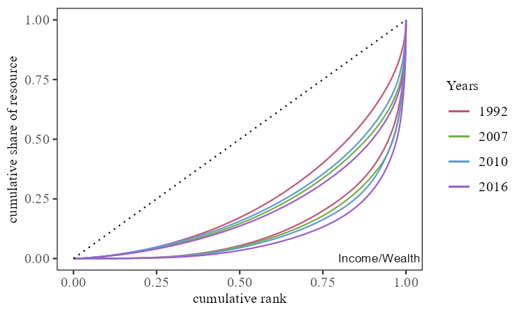
Figure 6. Univariate Lorenz curves for income (top cluster) and for wealth (bottom cluster) in the US for the years 1992, 2007, 2010, 2016.

Figure 7 displays univariate Gini indices for income and for wealth, the multivariate Gini index, as well as Kendall’s $\displaystyle\tau$ for the dependence between income and wealth over time. Contrary to the inconclusive evidence from univariate Lorenz curves, the multivariate Gini shows improved overall inequality between 2007 to 2010. More specifically the decreased correlation and income inequality was sufficient to offset the rise in wealth inequality. As another example, in 1992 and 1995, the drop in wealth inequality and correlation is offset by the increased income inequality, apparently increasing the multivariate Gini.

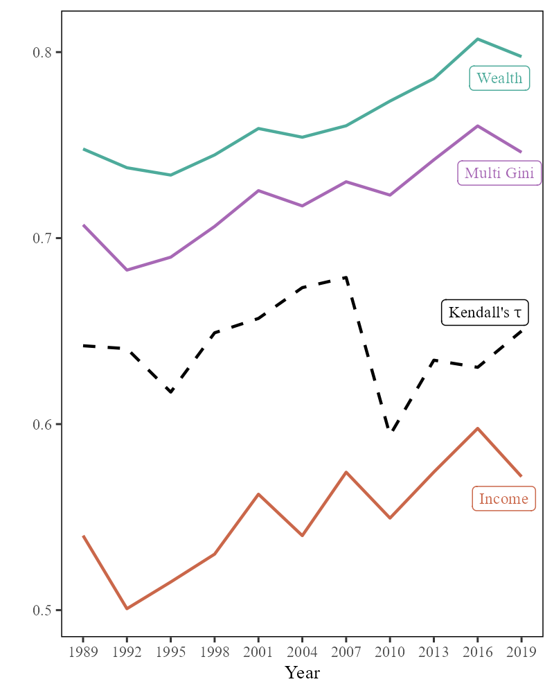
Figure 7. Gini indices for income and for wealth, multivariate Gini index, and Kendall’s $\displaystyle\tau$ for US Income-Wealth (dashed) between 1989 and 2019.

4.3. Discussion of $\displaystyle\alpha$-Lorenz curves for the SCF data

Figure 8 display the $\displaystyle 0.6$-, $\displaystyle 0.90$- and $\displaystyle 0.99$-Lorenz curves for the SCF data for the years 1992, 2007, 2010 and 2016 as well as the corresponding identical allocation curves. A common property for all clusters of curves is that they are disproportionately pulled towards the wealth axis and further away from the egalitarian curves indicating that wealth inequality is more pronounced than income inequality. For each year we see the effect on the curves of positive dependency through the curvature– the more curvature on the curve, the less positive dependence there is between the marginals. For example, for each $\displaystyle\alpha$-level the year 2016 has the most curvature and this intuition is supported by the Kendall’s $\displaystyle\tau$ in Figure 7 being the smallest value among these years.

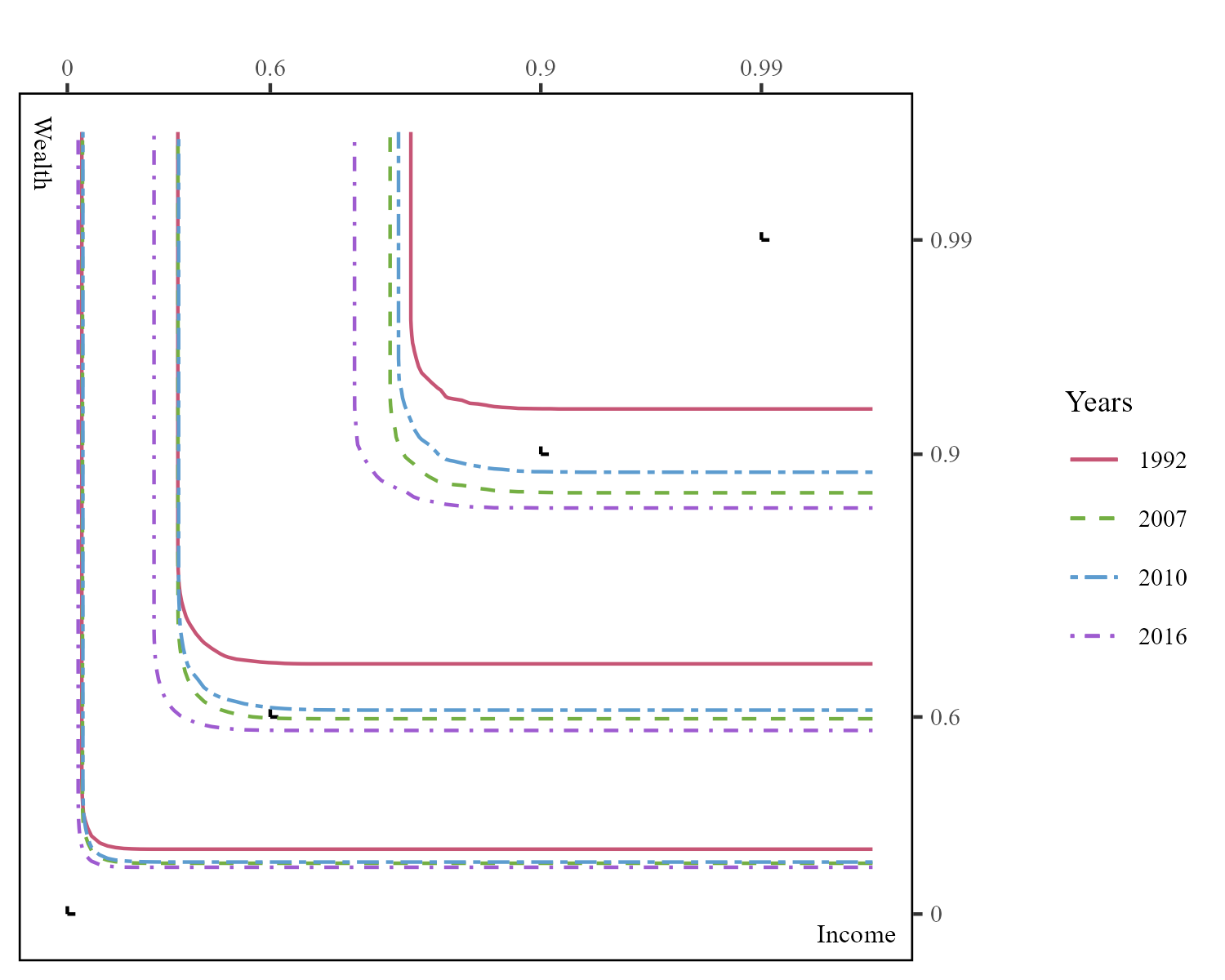
Figure 8. $\displaystyle\alpha$-Lorenz curves for US Income-Wealth for the years 1992, 2007, 2010, 2016, for $\displaystyle\alpha=0.6,0.9,0.99$. The horizontal-vertical scales are the $\displaystyle\alpha$-level of egalitarian $\displaystyle\alpha$-Lorenz curves. Black right-angle markings mark where the egalitarian Lorenz curves lie.

Visually there is a departure from the univariate Lorenz curves inconclusiveness in comparing overall inequality between 2007 and 2010. The $\displaystyle\alpha$-Lorenz curves suggest that overall inequality was higher in 2007 than in 2010 since the curves of 2010 are further shifted to the north-east. Therefore we have some suggestive evidence that the income-wealth allocation of 2007 is more unequal in the weak Lorenz order than the allocation in 2010. Overall, the ranking looks consistent with $\displaystyle X_{2016}\succcurlyeq_{l}X_{2007}\succcurlyeq_{l}X_{2010}\succcurlyeq_{l}X_{1992}$.

Appendix A Additional Details and Results

A.1. Vector ranks and quantiles

Proposition 3 below, a seminal result in the theory of measure transportation, states essential uniqueness of the gradient of a convex function (hence cyclically monotone map) that pushes the uniform distribution on $\displaystyle[0,1]^{2}$ into the distribution of an allocation $\displaystyle X$.

Proposition 3 (McCann 1995).

Let $\displaystyle P$ and $\displaystyle\lambda$ be two distributions on $\displaystyle\mathbb{R}^{d}$. ($\displaystyle i$) If $\displaystyle\lambda$ is absolutely continuous with respect to the Lebesgue measure on $\displaystyle\mathbb{R}^{d}$, with support contained in a convex set $\displaystyle\mathcal{U}$, the following statements hold: there exists a convex function $\displaystyle\psi:\mathcal{U}\rightarrow\mathbb{R}\cup\{+\infty\}$ such that $\displaystyle\nabla\psi_{\#}\lambda=P$. The function $\displaystyle\nabla\psi$ exists and is unique, $\displaystyle\lambda$-almost everywhere. ($\displaystyle ii$) If, in addition, $\displaystyle P$ is absolutely continuous on $\displaystyle\mathbb{R}^{d}$ with support contained in a convex set $\displaystyle\mathcal{X}$, the following holds: there exists a convex function $\displaystyle\psi^{\ast}:\mathcal{X}\rightarrow\mathbb{R}\cup\{+\infty\}$ such that $\displaystyle\nabla\psi^{\ast}_{\#}P=\lambda$. The function $\displaystyle\nabla\psi^{\ast}$ exists, is unique and equal to $\displaystyle\left(\nabla\psi\right)^{-1}$, $\displaystyle P$-almost everywhere.

Proposition 3 is an extension of Brenier (1991) (see also Rachev and Rüschendorf (1990)). It removes the finite variance requirement, which is undesirable in our context. Proposition 3 is the basis for the definition of vector quantiles and ranks in Chernozhukov et al. (2017). In our context, it is applied with uniform reference measure.

In case $\displaystyle d=1$, gradients of convex functions are nondecreasing functions, hence vector quantiles and ranks reduce to classical quantile and cumulative distribution functions. As the notation indicates, the function $\displaystyle\psi^{\ast}$ of proposition 3 is the convex conjugate of $\displaystyle\psi$. In case of absolutely continuous distributions $\displaystyle P$ on $\displaystyle\mathbb{R}^{d}$ with finite variance, the vector rank function solves a quadratic optimal transport problem, i.e., vector rank $\displaystyle R$ minimizes, among all functions $\displaystyle T$ such that $\displaystyle T(X)$ is uniform on $\displaystyle[0,1]^{d}$, the quantity $\displaystyle\mathbb{E}\|X-T(X)\|^{2}$, where $\displaystyle X\sim P$.

Appendix B Properties of the Gini coefficient

The Gini index of definition 8 is in $\displaystyle[0,1]$ under assumption 1. It satisfies a set desirable properties for an inequality index. The first two are explained in the main text and repeated here:

Property G1 (Anonymity). The Gini index of allocation $\displaystyle X$ is a function of the distribution $\displaystyle P_{X}$ of $\displaystyle X$.

Property G2 (Monotonicity). The Gini index is non decreasing in the Lorenz increasing inequality ordering. In other words, $\displaystyle X\preccurlyeq_{\mathcal{L}}\widetilde{X}$ implies $\displaystyle G(X)\leq G(\widetilde{X})$.

It also satisfies a multivariate extension of comonotonic independence proposed in Galichon and Henry (2012), as a generalization of the scalar requirement in Weymark (1981). Two scalar endowments $\displaystyle Y$ and $\displaystyle\widetilde{Y}$ are comonotonic if they are both increasing transformations of the same uniform random variable $\displaystyle V$ on $\displaystyle[0,1]$. Suppose $\displaystyle Y$ and $\displaystyle\widetilde{Y}$ have respective cdfs $\displaystyle F$ and $\displaystyle\widetilde{F}$. Then $\displaystyle Y$ and $\displaystyle\widetilde{Y}$ are comonotonic if they have the same ranks $\displaystyle V:=F(Y)=\widetilde{F}(\widetilde{Y})$.

Now, in case of random vectors $\displaystyle X$ and $\displaystyle\widetilde{X}$, comonotonicity is defined in the same way by the fact that $\displaystyle X$ and $\displaystyle\widetilde{X}$ have the same vector ranks. The following definition is due to Galichon and Henry (2012) and Ekeland et al. (2012), where it is called $\displaystyle\mu$-comonotonicity.

Definition 10 (Vector comonotonicity).

Random vectors $\displaystyle X_{1},\ldots,X_{J}$ on $\displaystyle\mathbb{R}^{2}$ are said to be comonotonic if there exists a uniform random vector $\displaystyle U$ on $\displaystyle[0,1]^{2}$ such that $\displaystyle X_{j}=\nabla\psi_{j}(U)$ almost surely, where $\displaystyle\nabla\psi_{j}$ is the vector quantile of definition 1 associated with the distribution of $\displaystyle X_{j}$, for each $\displaystyle j\leq J$.

The following property states that mixing two equally comonotonic endowments with the same third endowment, comonotonic with the first two, does not change the inequality ordering.

Property G3 (Comonotonic Independence). If $\displaystyle X$, $\displaystyle\widetilde{X}$ and $\displaystyle Z$ are comonotonic allocations, and $\displaystyle G(X)\leq G(\widetilde{X})$, then, for all $\displaystyle\mu\in(0,1)$, $\displaystyle G(\mu X+(1-\mu)Z)\leq G(\mu\widetilde{X}+(1-\mu)Z)$.

The interpretation of property G3 is very compelling for an inequality index. If individuals are ranked identically in endowments $\displaystyle X$ and $\displaystyle\widetilde{X}$, and $\displaystyle\widetilde{X}$ is more unequal than $\displaystyle X$, then, adding to both $\displaystyle X$ and $\displaystyle\widetilde{X}$ a third endowment $\displaystyle Z$ cannot reverse the inequality ordering, if $\displaystyle Z$ ranks individuals as $\displaystyle X$ and $\displaystyle\widetilde{X}$ do.

We bring these statements together in the following lemma:

Proposition 4.

The Gini index of definition 8 satisfies properties G1 to G3.

Proposition 4 is not a characterization of our proposed Gini index, even when we extend the definition to allow for different weights given to the different resources. In other words, there may be other inequality indices that also satisfy properties G1–3.

Property G2 is the preservation of the multivariate majorization order we introduce, based on multivariate rearrangements. Our multivariate Gini index preserves this majorization order, but not the traditional multivariate majorization of Kolm (1977). An example of multivariate Gini that satisfies properties G1, G3 and preserves the multivariate majorization order of Kolm (1977) is $\displaystyle\widetilde{G}(X):=\mathbb{E}[U^{\top}\nabla\psi_{X}(U)]-1$, proposed in Galichon and Henry (2012), where the expectation is taken with respect to $\displaystyle U\sim U[0,1]^{2}$. However, $\displaystyle\widetilde{G}$ is unsuitable as an inequality index in our context as can be seen with the following two observations. First, the following expression shows that $\displaystyle\widetilde{G}$ only depends on  $\displaystyle\mathcal{L}_{1}(p,1)+\mathcal{L}_{2}(1,p)$, hence, on very specific features of the dependence between the two components $\displaystyle X_{1}$ and $\displaystyle X_{2}$ of allocation $\displaystyle X$.

$$\displaystyle\widetilde{G}(X) \displaystyle= \displaystyle\int_{0}^{1}\Bigl{(}\left[p-\mathcal{L}_{1}\left(p,1\right)\right]+\left[p-\mathcal{L}_{2}\left(1,p\right)\right]\Bigr{)}\,dp.$$ (B.1)

Second, and more troubling still, for any given fixed marginals for $\displaystyle X_{1}$ and $\displaystyle X_{2}$, $\displaystyle\widetilde{G}$ is maximized when the two components $\displaystyle X_{1}$ and $\displaystyle X_{2}$ of endowment $\displaystyle X$ are independent, which runs against the intuition that increased dependence can increase inequality.

$$\displaystyle\widetilde{G}(X) \displaystyle\leq \displaystyle\frac{1}{2}\left[\,G\left(X_{1}\right)+G\left(X_{2}\right)\,\right],$$ (B.2)

where $\displaystyle G(X_{1})$ and $\displaystyle G(X_{2})$ denote the classical scalar Gini index of components $\displaystyle X_{1}$ and $\displaystyle X_{2}$ respectively.

Appendix C Specific features and issues with the data source

We review some known issues with the data set that impact our analysis. See Hanna et al. (2018) more a more in-depth account.

C.1. Sampling strategy

The over sampling of high income and wealthy households is achieved by applying two distinct sampling techniques. The first sample is the core representative sample selected by a standard multi-stage area-probability design. The second is the high income supplement from statistical records derived from tax data by the Statistics of Income (SOI) division of the Internal Revenue Service of the U.S. The stages sample disproportionately– usually one-third of the final sample is from the high income supplement. Sampling in this way retains characteristic information of the population while also addressing the known selection biases of the wealthy not responding to surveys. In order to represent the population with this sample, weights must be constructed for each unit of observation. For more details on the construction of weights and their implications on the distribution of wealth, see Kennickell and Woodburn (1999).

C.2. Unit of observation and timing of interviews

The observations in this data set are not households, but rather a subset called the primary economic unit (PEU) that may be individuals or couples and their financial dependents. For example in the 2016 data set 13% of PEUs were in a household that contained one or more members not in their PEU. Additionally, the respondent is not necessarily the head of the household, so special care must be taken if analyzing attitudes in relation to some demographic characteristics such as age. The interviews start in May of the survey year, after most income taxes are filed and usually finish by the end of the calendar year, see Kennickell (2017b) for challenges at the end of the interview period. Questions also may change over time so it is important to review the codebook each year when making comparisons across time.

C.3. Multiple Imputation

During interviews, respondents may omit answers or provide a range of values for which their response belongs. This missing data impacts analysis and so the SCF contains 5 imputed values for each PEU, creating a sample 5 times larger than the actual number of respondents and forms 5 data sets called implicates. Imputation is done by the Federal Reserve Imputation Technique Zeta model (FRITZ), details can be found in Kennickell (2017a) based upon the ideas of Little and Rubin (2019). Multiple imputation for missing data provide multiple probable values. Each of these form a data set from which sample statistics can be found. The technique of Repeated Imputation Inference (RII) is applied in our analysis. For each implicate $\displaystyle\ell=1,2,3,4,5$, the empirical ILF $\displaystyle\widehat{l}_{\ell*}$ is calculated using the appropriate quantile map estimator taking into account sample weights. Then the repeated-imputation estimate of $\displaystyle l$ is

$$\widehat{l}(z)=\frac{1}{5}\sum_{\ell=1}^{5}\widehat{l}_{\ell*}(z).$$

Calculation of the Gini index follows a similar procedure. Accounting for the multiple imputation in the calculation of standard errors is an important issue, but is not revelant to our visualization technique. For more information on multiple imputation and inference with imputed values, see Rubin (1996).

C.4. Computational issues

At times within the data, values can be repeated (e.g. many zeros), which have been found to pose issues calculating the quantile maps required for our Lorenz curves. Typically if this happens a few empty cells will be produced, which implies that the solution is invalid. A work-around for this is to introduce some noise to separate the data points. We added a random number between 0 and 10 for most implicates and added a random number between 0 and 200 to the data in 2007 and 2016. These numbers are too small to affect disparity when income and wealth are well over the tens of thousands in most of the stratum of the population so the visuals will not be influenced by this correction.

C.5. Definition of Wealth

In the literature, there is no consensus on what factors should be included in wealth measurement. Wolff (2021) defines wealth as marketable weath, which is the sum of marketable or fungible assets less the current value of all debts. Bricker et al. (2017) define wealth as net worth including those assets which are not readily transformed into consumption: properties, vehicles, etc. In our analysis we consider all assets, including financial, as our wealth variable.

Appendix D Proofs of results in the main text

In this section, we omit the $\displaystyle X$ subscript of $\displaystyle\psi_{X}$ for notational compactness.

D.1. Proofs for section 1.3

Proof of property 1.

The off diagonal elements of the Jacobian of $\displaystyle\mathcal{L}(r)$ are $\displaystyle\psi(r_{1},r_{2})-\psi(r_{1},0)$ and $\displaystyle\psi(r_{1},r_{2})-\psi(0,r_{2})$. From the latter, by differentiation, we can recover $\displaystyle\nabla\psi(r_{1},r_{2})$. The result then follows from the fact that $\displaystyle\nabla\psi$ characterizes $\displaystyle P_{X}$, see for instance Chernozhukov et al. (2017). ∎

Proof of lemma 1.

Let $\displaystyle U\sim U[0,1]^{2}$. Let $\displaystyle\widetilde{X}_{j}:=\frac{\partial\psi}{\partial u_{j}}(U_{1},U_{2})$, $\displaystyle j=1,2$. Then $\displaystyle(\widetilde{X}_{1},\widetilde{X}_{2})$ is distributed identically to $\displaystyle(X_{1},X_{2})$. Since $\displaystyle\widetilde{X}_{2}=\frac{\partial\psi}{\partial u_{2}}(U_{1},U_{2})$ is monotonically increasing in $\displaystyle U_{2}$, we have $\displaystyle U_{2}=\left(\frac{\partial\psi}{\partial u_{2}}\right)^{-1}(U_{1},\widetilde{X}_{2})$. Hence

$$\displaystyle\widetilde{X}_{1} \displaystyle= \displaystyle\frac{\partial\psi}{\partial u_{1}}\left(U_{1},\left(\frac{\partial\psi}{\partial u_{2}}\right)^{-1}(U_{1},\widetilde{X}_{2})\right).$$

Under the stated assumption, $\displaystyle\widetilde{X}_{1}$ is increasing in $\displaystyle U_{1}$ and $\displaystyle\widetilde{X}_{2}$. Since $\displaystyle\left(\widetilde{X}_{1},\widetilde{X}_{2}\right)\overset{d}{=}\left(X_{1},X_{2}\right)$, we have

$$\displaystyle F_{X}\left(x_{1},x_{2}\right) \displaystyle= \displaystyle\mathbb{P}\left(\widetilde{X}_{1}\leq x_{1},\widetilde{X}_{2}\leq x_{2}\right)$$

$$\displaystyle= \displaystyle\mathbb{E}\bigg{[}\mathbb{P}\left(\frac{\partial\psi}{\partial u_{1}}\left(U_{1},\left(\frac{\partial\psi}{\partial u_{2}}\right)^{-1}(U_{1},\widetilde{X}_{2})\right)\leq x_{1},\widetilde{X}_{2}\leq x_{2}\right)\bigg{|}\;U_{1}\bigg{]}$$

$$\displaystyle= \displaystyle\mathbb{E}\left[\min\left\{F_{1}\left(x_{1}|U_{1}\right),F_{2}\left(x_{2}|U_{1}\right)\right\}\right]$$

$$\displaystyle\geq \displaystyle\mathbb{E}\left[F_{1}\left(x_{1}|U_{1}\right)F_{2}\left(x_{2}|U_{1}\right)\right],$$

where $\displaystyle F_{i}(\cdot|U_{j})$ denotes the cumulative distribution function of $\displaystyle X_{i}$ conditional on $\displaystyle U_{j}$. Now $\displaystyle F_{1}\left(x_{1}|U_{1}\right)$ is increasing in $\displaystyle U_{1}$, since

$$\displaystyle F_{1}\left(x_{1}|U_{1}\right) \displaystyle= \displaystyle\mathbb{P}\left(\frac{\partial\psi}{\partial u_{1}}(U_{1},U_{2})\leq x_{1}\bigg{|}\;U_{1}\right)$$

$$\displaystyle= \displaystyle\mathbb{P}\left(U_{2}\leq\left(\frac{\partial\psi}{\partial u_{1}}\right)^{-1}(U_{1},x_{1})\bigg{|}\;U_{1}\right)$$

$$\displaystyle= \displaystyle\left(\frac{\partial\psi}{\partial u_{1}}\right)^{-1}(U_{1},x_{1}).$$

Similarly $\displaystyle F_{2}\left(x_{2}|U_{1}\right)$ is increasing in $\displaystyle U_{1}$. We conclude that $\displaystyle F_{X}\left(x_{1},x_{2}\right)\geq F_{1}\left(x_{1}\right)F_{2}\left(x_{2}\right)$, see e.g. Joe (1997). ∎

Proof of property 3.

We only need to show for one component of the Lorenz map and the second follows with similar reasoning. We have for the first component

$$\displaystyle\mathcal{L}_{1}(r) \displaystyle= \displaystyle\int_{0}^{r_{2}}\int_{0}^{r_{1}}\frac{\partial\psi}{\partial u_{1}}(u_{1},u_{2})du_{1}du_{2}$$

$$\displaystyle= \displaystyle\int_{0}^{r_{2}}[\psi(r_{1},u_{2})-\psi(0,u_{2})]du_{2}$$

$$\displaystyle\leq \displaystyle\int_{0}^{r_{2}}r_{1}[\psi(1,u_{2})-\psi(0,u_{2})]du_{2}\text{, by convexity }$$

$$\displaystyle= \displaystyle r_{1}\int_{0}^{r_{2}}\int_{0}^{1}\frac{\partial\psi}{\partial u_{1}}(u_{1},u_{2})du_{1}du_{2}$$

Now define $\displaystyle H(r_{2})=\int_{0}^{r_{2}}\int_{0}^{1}\frac{\partial\psi}{\partial u_{1}}(u_{1},u_{2})du_{1}du_{2}$. $\displaystyle H^{\prime}(r_{2})=\int_{0}^{1}\frac{\partial\psi}{\partial u_{1}}(u_{1},r_{2})du_{1}$ is monotone increasing by assumption, so $\displaystyle H$ is convex. Therefore, $\displaystyle H(r_{2})\leq H(0)+r_{2}(H(1)-H(0))$. Note that $\displaystyle H(0)=0$ as an integral over a degenerate interval, and $\displaystyle H(1)=1$, as this is the mean of the normalized $\displaystyle X_{1}$. So $\displaystyle H(r_{2})\leq r_{2}$ and so $\displaystyle\mathcal{L}_{1}(r)\leq r_{1}r_{2}$, as desired. ∎

Proof of property 4.

(i) Let $\displaystyle l_{X}(z_{1},z_{2})=\alpha$. Since $\displaystyle l_{X}$ is a cdf, hence non decreasing in both arguments, the generalized inverse $\displaystyle z_{2}:=l_{X}^{-1}(z_{1};\alpha)$ is non increasing in $\displaystyle z_{1}$ non decreasing in $\displaystyle\alpha$. (ii) See Claim 1 in Brock and Thomson (1966). ∎

D.2. Proofs for section 2

Proof of proposition 1.

$\displaystyle\widetilde{X}\succcurlyeq_{\mathcal{L}}X$ is equivalent to first order stochastic dominance of $\displaystyle\mathcal{L}_{X}(U)$ over $\displaystyle\mathcal{L}_{\widetilde{X}}(U)$, where $\displaystyle U\sim U[0,1]^{d}$ (see Section 6.B page 266 of Shaked and Shanthikumar (2007)). Hence, $\displaystyle\widetilde{X}\succcurlyeq_{\mathcal{L}}X$ implies $\displaystyle\mathbb{P}(\mathcal{L}_{X}(U)\in S)\leq\mathbb{P}(\mathcal{L}_{\widetilde{X}}(U)\in S)$ for any lower set $\displaystyle S$, so that $\displaystyle\widetilde{X}\succcurlyeq_{\mathcal{L}}X$ implies $\displaystyle\widetilde{X}\succcurlyeq_{l}X$, given that the sets $\displaystyle[0,z]$ are lower sets. ∎

Proof of lemma 2.

Suppose $\displaystyle Y$ is an MMPS of $\displaystyle X$, so that there is an ultramodular function $\displaystyle\psi$, such that (2.1) holds, with $\displaystyle\int\!\!\!\int^{1}\nabla\psi(u)du=0$ (since $\displaystyle\mathbb{E}[Y]=\mathbb{E}[X]$ by assumption). We want to see if $\displaystyle\mathcal{L}_{Y}\leq\mathcal{L}_{X}$, i.e., $\displaystyle\int\!\!\!\int^{r}\nabla\psi(u)du\leq 0$. Consider the first component:

$$\displaystyle\int\!\!\!\int^{r}\nabla\psi(u)du \displaystyle= \displaystyle\int^{r_{2}}[\psi(r_{1},u_{2})-\psi(0,u_{2})]du_{2}$$

$$\displaystyle\leq \displaystyle r_{1}\int^{r_{2}}[\psi(1,u_{2})-\psi(0,u_{2})]du_{2},$$

by convexity. We then show that

$$\displaystyle f(r_{2}) \displaystyle= \displaystyle\int^{r_{2}}[\psi(1,u_{2})-\psi(0,u_{2})]du_{2}\leq 0$$

for all $\displaystyle r_{2}\in[0,1]$. Since $\displaystyle f(0)=f(1)=0$, the latter holds if $\displaystyle f$ is convex, i.e., if

$$\displaystyle f^{{}^{\prime\prime}}(r_{2}) \displaystyle= \displaystyle\frac{\partial}{\partial r_{2}}[\psi(1,r_{2})-\psi(0,r_{2})]$$

$$\displaystyle= \displaystyle\frac{\partial}{\partial r_{2}}\int_{0}^{1}\frac{\partial}{\partial r_{1}}\psi(r_{1},r_{2})dr_{1}$$

$$\displaystyle= \displaystyle\int_{0}^{1}\frac{\partial^{2}}{\partial r_{1}\partial r_{2}}\psi(r_{1},r_{2})dr_{1}$$

$$\displaystyle\geq \displaystyle 0,$$

which holds by supermodularity of $\displaystyle\psi$. A similar reasoning applies to the second component and the result follows. ∎

Proof of proposition 4.

Property  G1 is automatically satisfied since $\displaystyle G$ is defined as a function of the allocation’s distribution. Property G2 follows immediately from equation 2.6. We now show that Property G3 is satisfied. Take $\displaystyle\mu\in(0,1)$. Let $\displaystyle X$, $\displaystyle\widetilde{X}$ and $\displaystyle Z$ be comonotonic according to definition 10, and assume $\displaystyle G(X)\leq G(\widetilde{X})$, i.e., $\displaystyle\mathbb{E}[\mathcal{L}_{X}(R)]\geq\mathbb{E}[\mathcal{L}_{X}(R)]$. We have

$$\displaystyle\mathbb{E}[(1\;1)^{\top}\mathcal{L}_{\mu X+(1-\mu)Z}(R)] \displaystyle= \displaystyle\int_{r\in[0,1]^{2}}\int_{u\in[0,r]}(1\;1)^{\top}\nabla\psi_{\mu X+(1-\mu)Z}(u)\,dudr$$

$$\displaystyle= \displaystyle\int_{r\in[0,1]^{2}}\int_{u\in[0,r]}(1\;1)^{\top}\left(\mu\nabla\psi_{X}(u)+(1-\mu)\nabla\psi_{Z}(u)\right)\,dudr$$

$$\displaystyle= \displaystyle\mu\mathbb{E}[(1\;1)^{\top}\mathcal{L}_{X}(R)]+(1-\mu)\mathbb{E}[(1\;1)^{\top}\mathcal{L}_{Z}(R)]$$

$$\displaystyle\geq \displaystyle\mu\mathbb{E}[(1\;1)^{\top}\mathcal{L}_{\widetilde{X}}(R)]+(1-\mu)\mathbb{E}[(1\;1)^{\top}\mathcal{L}_{Z}(R)]$$

$$\displaystyle= \displaystyle\mathbb{E}[(1\;1)^{\top}\mathcal{L}_{\mu\widetilde{X}+(1-\mu)Z}(R)]$$

where the second and last equalities hold by lemma 4. The result follows. ∎

Lemma 4 (Galichon and Henry (2012)).

If $\displaystyle X$ and $\displaystyle Z$ with respective vector quantiles $\displaystyle\nabla\psi_{X}$ and $\displaystyle\nabla\psi_{Z}$ are comonotonic, then, for any $\displaystyle\mu\in(0,1)$, the vector quantile of $\displaystyle\mu X+(1-\mu)Z$ is $\displaystyle\mu\nabla\psi_{X}+(1-\mu)\nabla\psi_{Z}$.

Proof of (B.1).

Let $\displaystyle U$ be uniformly distributed on $\displaystyle[0,1]^{2}$. Note that

$$\displaystyle\widetilde{G}(X) \displaystyle= \displaystyle\mathbb{E}\left[U_{1}\frac{\partial\psi}{\partial u_{1}}(U_{1},U_{2})\right]+\mathbb{E}\left[U_{1}\frac{\partial\psi}{\partial u_{1}}(U_{1},U_{2})\right]-1.$$

Now,

$$\displaystyle\mathbb{E}\left[U_{1}\frac{\partial\psi}{\partial u_{1}}(U_{1},U_{2})\right] \displaystyle= \displaystyle\int_{0}^{1}\left[\int_{0}^{1}u_{1}\frac{\partial\psi}{\partial u_{1}}(u_{1},u_{2})\,du_{1}\right]du_{2}$$

$$\displaystyle= \displaystyle\int_{0}^{1}\left[\int_{0}^{1}u_{1}\,d\left(\frac{\partial\mathcal{L}_{1}}{\partial u_{2}}(u_{1},u_{2})\right]\,\right)du_{2}$$

where the last equality follows from interchangeability of the order of integration and $\displaystyle\mathcal{L}_{1}$ is the first component of the Lorenz map.

Note that

$$\displaystyle\frac{\partial\mathcal{L}_{1}}{\partial r_{2}}(r_{1},r_{2}) \displaystyle= \displaystyle\int_{0}^{r_{1}}\frac{\partial\psi}{\partial u_{1}}(u_{1},u_{2})\,du_{1}$$

and

$$\displaystyle\frac{\partial}{\partial r_{1}}\left(\frac{\partial\mathcal{L}_{1}(r_{1},r_{2})}{\partial r_{2}}\right) \displaystyle= \displaystyle\frac{\partial\psi}{\partial u_{1}}(r_{1},r_{2}).$$

Therefore

$$\displaystyle\mathbb{E}\left[U_{1}\frac{\partial\psi}{\partial u_{1}}(U_{1},U_{2})\right] \displaystyle= \displaystyle\int_{0}^{1}\left(u_{1}\frac{\partial\mathcal{L}_{1}}{\partial u_{2}}(u_{1},u_{2})\bigg{|}_{0}^{1}-\int_{0}^{1}\frac{\partial\mathcal{L}_{1}}{\partial u_{2}}(u_{1},u_{2})\,du_{1}\right)\,du_{2}$$

$$\displaystyle= \displaystyle\int_{0}^{1}\left(\frac{\partial\mathcal{L}_{1}}{\partial u_{2}}(1,u_{2})-\int_{0}^{1}\frac{\partial\mathcal{L}_{1}}{\partial u_{2}}(u_{1},u_{2})\,du_{1}\right)\,du_{2}$$

$$\displaystyle= \displaystyle\int_{0}^{1}\frac{\partial\mathcal{L}_{1}}{\partial u_{2}}(1,u_{2})\,du_{2}-\int_{0}^{1}\int_{0}^{1}\frac{\partial\mathcal{L}_{1}}{\partial u_{2}}(u_{1},u_{2})\,du_{2}\,du_{1}$$

$$\displaystyle= \displaystyle\mathcal{L}(1,1)-\mathcal{L}(1,0)-\int_{0}^{1}\mathcal{L}_{1}(u_{1},1)-\mathcal{L}_{1}(u_{1},0)\,du_{1}$$

$$\displaystyle= \displaystyle 1-\int_{0}^{1}\mathcal{L}_{1}(u_{1},1)\,du_{1}.$$

Similarly, we have $\displaystyle\mathbb{E}\left[U_{2}\frac{\partial\psi}{\partial u_{2}}(U_{1},U_{2})\right]=1-\int_{0}^{1}\mathcal{L}_{2}(1,u_{2})\,du_{1}$, as desired. ∎

Proof of (B.2).

$\displaystyle 0\leq\widetilde{G}(X)$ because $\displaystyle p\geq\mathcal{L}_{1}\left(p,1\right)$ and $\displaystyle p\geq\mathcal{L}_{2}\left(1,p\right)$. The second inequality follows from $\displaystyle\mathcal{L}_{1}\left(p,1\right)\geq L_{1}\left(p\right)$ and $\displaystyle\mathcal{L}_{2}\left(1,p\right)\geq L_{2}\left(p\right)$. We now prove the latter. Letting $\displaystyle\nabla\psi$ be the vector quantile function of $\displaystyle(X_{1},X_{2})$, note that since $\displaystyle\frac{\partial\psi}{\partial u_{1}}$ pushes uniform measure on $\displaystyle[0,1]^{2}$ forward to law$\displaystyle(X_{1})$, we can write

$$L_{1}(r_{1})=\int_{\{u:\frac{\partial\psi}{\partial u_{1}}(u)\leq z_{1}(r_{1})\}}\frac{\partial\psi}{\partial u_{1}}(u)du$$

where $\displaystyle z_{1}(r_{1})$ is the quantile of the random variable $\displaystyle X_{1}$. Note that the area of the domain $\displaystyle\{u:\frac{\partial\psi}{\partial u_{1}}(u)\leq z_{1}(r_{1})\}$ of integration must be $\displaystyle r_{1}$. On the other hand,

$$\mathcal{L}_{1}(r_{1},1)=\int_{0}^{r_{1}}\int_{0}^{1}\frac{\partial\psi}{\partial u_{1}}(u)du_{1}du_{2}$$

is an integral of the same function over a region with the same area. Writing $\displaystyle A:=\left\{u:\frac{\partial\psi}{\partial u_{1}}(u)\leq z_{1}(r_{1})\right\}$, we have $\displaystyle A=B\cup C$, where $\displaystyle B=A\cap([0,r_{1}]\times[0,1])$ and $\displaystyle C=A\cap((r_{1},1]\times[0,1])$ and the union is disjoint. Similarly, $\displaystyle[0,r_{1}]\times[0,1]=B\cup D$ where $\displaystyle D=([0,r_{1}]\times[0,1])\cap A^{c}$. Note that the areas of $\displaystyle C$ and $\displaystyle D$ must be the same, $\displaystyle|C|=|D|$, and $\displaystyle\frac{\partial\psi}{\partial u_{1}}(u)\leq z_{1}(r_{1})$ throughout $\displaystyle C$ while $\displaystyle\frac{\partial\psi}{\partial u_{1}}(u)>z_{1}(r_{1})$ throughout $\displaystyle D$. We have

$$\displaystyle L_{1}(r_{1})1=L_{1}(r_{1}) \displaystyle= \displaystyle\int_{B}\frac{\partial\psi}{\partial u_{1}}(u)du+\int_{C}\frac{\partial\psi}{\partial u_{1}}(u)du$$

$$\displaystyle\leq \displaystyle\int_{B}\frac{\partial\psi}{\partial u_{1}}(u)du+z_{1}(r_{1})|C|$$

$$\displaystyle= \displaystyle\int_{B}\frac{\partial\psi}{\partial u_{1}}(u)du+z_{1}(r_{1})|D|$$

$$\displaystyle\leq \displaystyle\int_{B}\frac{\partial\psi}{\partial u_{1}}(u)du+\int_{D}\frac{\partial\psi}{\partial u_{1}}(u)du$$

$$\displaystyle= \displaystyle\mathcal{L}_{1}(r_{1},1).$$

Note that this inequality holds for any dependence structure between $\displaystyle X_{1}$ and $\displaystyle X_{2}$. ∎

Lemma 5.

For non negative bivariate random vectors $\displaystyle X$ with $\displaystyle\mathbb{E}[X]=(1,1)$, we have

$$\displaystyle\mathbb{E}[\mathcal{L}_{1}(U_{1},U_{2})]=1-\mathbb{E}\bigg{[}U_{2}\frac{\partial\psi(U)}{\partial U_{1}}\bigg{]}-\mathbb{E}\bigg{[}U_{1}\frac{\partial\psi(U)}{\partial U_{1}}\bigg{]}+\mathbb{E}\bigg{[}U_{1}U_{2}\frac{\partial\psi(U)}{\partial U_{1}}\bigg{]}$$

$$\displaystyle\mathbb{E}[\mathcal{L}_{2}(U_{1},U_{2})]=1-\mathbb{E}\bigg{[}U_{1}\frac{\partial\psi(U)}{\partial U_{2}}\bigg{]}-\mathbb{E}\bigg{[}U_{2}\frac{\partial\psi(U)}{\partial U_{2}}\bigg{]}+\mathbb{E}\bigg{[}U_{1}U_{2}\frac{\partial\psi(U)}{\partial U_{2}}\bigg{]}$$

where $\displaystyle(U_{1},U_{2})\sim U([0,1]^{2})$.

Proof of lemma 5.

This is seen by applying integration by parts a few times. Start with

$$\displaystyle\mathbb{E}[\mathcal{L}_{1}(U_{1},U_{2})] \displaystyle=\int_{0}^{1}\int_{0}^{1}\int_{0}^{r_{2}}\int_{0}^{r_{1}}\frac{\partial\psi(u_{1},u_{2})}{\partial u_{1}}\,du_{1}du_{2}dr_{1}dr_{2}$$

$$\displaystyle=\int_{0}^{1}\int_{0}^{r_{2}}\int_{0}^{1}\int_{0}^{r_{1}}\frac{\partial\psi(u_{1},u_{2})}{\partial u_{1}}\,du_{1}dr_{1}du_{2}dr_{2}$$

$$\displaystyle=\int_{0}^{1}\int_{0}^{r_{2}}\bigg{(}r_{1}\int_{0}^{r_{1}}\frac{\partial\psi(u_{1},u_{2})}{\partial u_{1}}\,du_{1}\bigg{|}_{0}^{1}-\int_{0}^{1}r_{1}\frac{\partial\psi(r_{1},u_{2})}{\partial u_{1}}\,dr_{1}\bigg{)}\,du_{2}dr_{2}$$

$$\displaystyle=\underbrace{\int_{0}^{1}\int_{0}^{r_{2}}\int_{0}^{1}\frac{\partial\psi(u_{1},u_{2})}{\partial u_{1}}\,du_{1}\,du_{2}dr_{2}}_{A}-\underbrace{\int_{0}^{1}\int_{0}^{r_{2}}\int_{0}^{1}r_{1}\frac{\partial\psi(r_{1},u_{2})}{\partial u_{1}}\,dr_{1}\,du_{2}dr_{2}}_{B}.$$

Then

$$\displaystyle A \displaystyle= \displaystyle\int_{0}^{1}\int_{0}^{1}\int_{0}^{r_{2}}\frac{\partial\psi(u_{1},u_{2})}{\partial u_{1}}\,du_{2}dr_{2}du_{1}$$

$$\displaystyle= \displaystyle\int_{0}^{1}\bigg{(}r_{2}\int_{0}^{r_{2}}\frac{\partial\psi(u_{1},u_{2})}{\partial u_{1}}\,du_{2}\bigg{|}_{0}^{1}\ -\int_{0}^{1}r_{2}\frac{\partial\psi(u_{1},r_{2})}{\partial u_{1}}\,dr_{2}\bigg{)}\,du_{1}$$

$$\displaystyle= \displaystyle\int_{0}^{1}\int_{0}^{1}\frac{\partial\psi(u_{1},u_{2})}{\partial u_{1}}\,du_{2}\,du_{1}-\int_{0}^{1}\int_{0}^{1}r_{2}\frac{\partial\psi(u_{1},r_{2})}{\partial u_{1}}\,dr_{2}du_{1}$$

$$\displaystyle= \displaystyle\mathbb{E}\bigg{[}\frac{\partial\psi(U)}{\partial u_{1}}\bigg{]}-\mathbb{E}\bigg{[}U_{2}\frac{\partial\psi(U)}{\partial u_{1}}\bigg{]}$$

$$\displaystyle= \displaystyle 1-\mathbb{E}\bigg{[}U_{2}\frac{\partial\psi(U)}{\partial u_{1}}\bigg{]}$$

and

$$\displaystyle B \displaystyle= \displaystyle\int_{0}^{1}\int_{0}^{1}\int_{0}^{r_{2}}r_{1}\frac{\partial\psi(r_{1},u_{2})}{\partial u_{1}}\,du_{2}\,dr_{2}dr_{1}$$

$$\displaystyle= \displaystyle\int_{0}^{1}r_{1}\bigg{(}r_{2}\int_{0}^{r_{2}}\frac{\partial\psi(r_{1},u_{2})}{\partial u_{1}}\,du_{2}\bigg{|}_{0}^{1}-\int_{0}^{1}r_{2}\frac{\partial\psi(r_{1},r_{2})}{\partial u_{1}}\,dr_{2}\bigg{)}\,dr_{1}$$

$$\displaystyle= \displaystyle\int_{0}^{1}\int_{0}^{1}r_{1}\frac{\partial\psi(r_{1},u_{2})}{\partial u_{1}}\,du_{2}dr_{1}-\int_{0}^{1}\int_{0}^{1}r_{1}r_{2}\frac{\partial\psi(r_{1},r_{2})}{\partial u_{1}}\,dr_{2}dr_{1}$$

$$\displaystyle= \displaystyle\mathbb{E}\bigg{[}U_{1}\frac{\partial\psi(U)}{\partial u_{1}}\bigg{]}-\mathbb{E}\bigg{[}U_{1}U_{2}\frac{\partial\psi(U)}{\partial u_{1}}\bigg{]}.$$

Combining these,

$$\mathbb{E}[\mathcal{L}_{1}(U_{1},U_{2})]=1-\mathbb{E}\bigg{[}U_{2}\frac{\partial\psi(U)}{\partial u_{1}}\bigg{]}-\mathbb{E}\bigg{[}U_{1}\frac{\partial\psi(U)}{\partial u_{1}}\bigg{]}+\mathbb{E}\bigg{[}U_{1}U_{2}\frac{\partial\psi(U)}{\partial u_{1}}\bigg{]}.$$

It is a similar line of reasoning for the second component. ∎

Proof of (2.7).

Using lemma 5, we can rewrite $\displaystyle G$ as

$$\displaystyle G(X) \displaystyle= \displaystyle 2\bigg{(}\mathbb{E}[U^{\top}\nabla\psi(U)]+\mathbb{E}\bigg{[}U_{2}(1-U_{1})\frac{\partial\psi(U)}{\partial u_{1}}\bigg{]}+\mathbb{E}\bigg{[}U_{1}(1-U_{2})\frac{\partial\psi(U)}{\partial u_{2}}\bigg{]}\bigg{)}-3$$

$$\displaystyle= \displaystyle 2\,\mathbb{E}\left[(U_{1}+U_{2}-U_{1}U_{2})\left(\frac{\partial\psi(U)}{\partial u_{1}}+\frac{\partial\psi(U)}{\partial u_{2}}\right)\right]\,-\,3,$$

which is the desired result. ∎

D.3. Proofs for section 3

Proof of proposition 2.

The potential $\displaystyle\psi$ of an egalitarian allocation satisfies $\displaystyle\partial\psi/\partial u_{1}+p\partial\psi/\partial u_{2}=1+p$. Solutions are of the form

$$\displaystyle\psi_{(v,p)}(u_{1},u_{2})=u_{1}+u_{2}+v(pu_{1}-u_{2}).$$

Convexity of $\displaystyle\psi$ implies convexity of $\displaystyle v$. The normalization

$$\displaystyle\int_{0}^{1}\!\!\!\int_{0}^{1}\nabla\psi_{(v,p)}(u_{1},u_{2})du_{1}du_{2}=(1,1)$$

implies

$$\displaystyle\int_{0}^{1}\!\!\!\int_{0}^{1}v^{\prime}(pu_{1}-u_{2})du_{1}du_{2}=0.$$

The latter, in turn, implies

$$\displaystyle\int_{0}^{1}v(p-x)dx=\int_{0}^{1}v(x)dx.$$

Call $\displaystyle H_{p}$ the cdf of $\displaystyle Z=pU_{1}-U_{2}$, where $\displaystyle(U_{1},U_{2})\sim U[0,1]^{2}$. Call $\displaystyle F_{1}$ the cdf of $\displaystyle\nabla_{1}\psi_{(p,v)}:=1+pv^{\prime}(Z)$, which is the first marginal of allocation $\displaystyle X$. Then

$$\displaystyle F_{1}(x) \displaystyle= \displaystyle\mathbb{P}\left(v^{\prime}(Z)\leq\frac{x-1}{p}\right)$$

$$\displaystyle= \displaystyle\mathbb{P}\left(Z\leq(v^{\prime})^{-1}\left(\frac{x-1}{p}\right)\right)$$

$$\displaystyle= \displaystyle H_{p}\left((v^{\prime})^{-1}\left(\frac{x-1}{p}\right)\right).$$

Now

$$\displaystyle F_{1}(x)=H_{p}\left((v^{\prime})^{-1}\left(\frac{x-1}{p}\right)\right) \displaystyle\Rightarrow \displaystyle(v^{\prime})^{-1}\left(\frac{x-1}{p}\right)=H_{p}^{-1}\left(F_{1}(x)\right)$$

$$\displaystyle\Rightarrow \displaystyle\frac{x-1}{p}=v^{\prime}\left(H_{p}^{-1}\left(F_{1}(x)\right)\right)$$

$$\displaystyle\Rightarrow \displaystyle v^{\prime}(z)=\frac{F_{1}^{-1}(H_{p}(z))-1}{p}.$$

Hence

$$\displaystyle v(z) \displaystyle= \displaystyle\int_{0}^{x}\frac{F_{1}^{-1}(H_{p}(y))-1}{p}dy,$$

as desired. ∎

Lemma 6 (Explicit formula for $\displaystyle H_{p}(z)$).

The cumulative distribution function of $\displaystyle Z=pU_{1}-U_{2}$ with $\displaystyle(U_{1},U_{2})\sim U[0,1]^{2}$ is given by the following.

$$\displaystyle H_{p}(z) \displaystyle= \displaystyle\left\{\begin{array}[]{llc}1&\mbox{if}&p<z,\\ \\ 1-\frac{p}{2}+z-\frac{z^{2}}{2p}&\mbox{if}&\max\{p-1,0\}<z\leq p,\\ \\ \frac{1+2z}{2p}&\mbox{if}&0<z\leq\max\{p-1,0\},\\ \\ 1-\frac{p}{2}+z&\mbox{if}&\min\{p-1,0\}<z\leq 0,\\ \\ \frac{1}{p}\left(\frac{1}{2}+z+\frac{z^{2}}{2}\right)&\mbox{if}&-1<z\leq\min\{p-1,0\},\\ \\ 0&\mbox{if}&z\leq-1.\end{array}\right.$$

Proof of lemma 3.

A sufficient condition for assumption 2 is

$$\displaystyle-\inf_{u_{1},u_{2}}\frac{1}{p}\frac{\partial^{2}\psi_{X}(u_{1},u_{2})}{\partial u_{1}\partial u_{2}}\leq\min\left\{\inf_{u_{1},u_{2}}\frac{1}{p^{2}}\frac{\partial^{2}\psi_{X}(u_{1},u_{2})}{\partial u_{1}^{2}},\inf_{u_{1},u_{2}}\frac{\partial^{2}\psi_{X}(u_{1},u_{2})}{\partial u_{2}^{2}}\right\}.$$

If we choose the optimal value of $\displaystyle p$, i.e.,

$$\displaystyle p^{2}=\frac{\inf_{u_{1},u_{2}}\frac{\partial^{2}\psi_{X}(u_{1},u_{2})}{\partial u_{1}^{2}}}{\inf_{u_{1},u_{2}}\frac{\partial^{2}\psi_{X}(u_{1},u_{2})}{\partial u_{2}^{2}}},$$

we get the sufficient inequality

$$\displaystyle-\inf_{u_{1},u_{2}}\frac{\partial^{2}\psi_{X}(u_{1},u_{2})}{\partial u_{1}\partial u_{2}}\leq\sqrt{\inf_{u_{1},u_{2}}\frac{\partial^{2}\psi_{X}(u_{1},u_{2})}{\partial u_{1}^{2}}\times\inf_{u_{1},u_{2}}\frac{\partial^{2}\psi_{X}(u_{1},u_{2})}{\partial u_{2}^{2}}}$$

as desired. ∎

Proof of example 1.

Let $\displaystyle\psi(u_{1},u_{2})=u_{1}+u_{2}+v(pu_{1}-u_{2})+\widetilde{\psi}(u_{1},u_{2})$, with $\displaystyle v$ convex and twice continuously differentiable, and $\displaystyle\psi$ ultramodular. We have, for $\displaystyle j=1,2,$

$$\displaystyle\begin{array}[]{lll}\frac{\partial^{2}\psi(u_{1},u_{2})}{\partial u_{1}^{2}}&=&p^{2}v^{\prime\prime}(pu_{1}-u_{2})+\frac{\partial^{2}\widetilde{\psi}(u_{1},u_{2})}{\partial u_{2}^{2}},\\ \\ \frac{\partial^{2}\psi(u_{1},u_{2})}{\partial u_{1}^{2}}&=&v^{\prime\prime}(pu_{1}-u_{2})+\frac{\partial^{2}\widetilde{\psi}(u_{1},u_{2})}{\partial u_{2}^{2}}.\end{array}$$

Also,

$$\displaystyle\begin{array}[]{lll}\frac{\partial^{2}\psi(u_{1},u_{2})}{\partial u_{1}\partial u_{2}}&=&-pv^{\prime\prime}(pu_{1}-u_{2})+\frac{\partial^{2}\widetilde{\psi}(u_{1},u_{2})}{\partial u_{1}\partial u_{2}}.\end{array}$$

Therefore

$$\displaystyle\begin{array}[]{rll}\sup_{pu_{1}-u_{2}=z}\left\{-\frac{1}{p}\frac{\partial^{2}\psi(u_{1},u_{2})}{\partial u_{1}\partial u_{2}}\right\}&=&\sup_{pu_{1}-u_{2}=z}\left\{v^{\prime\prime}(pu_{1}-u_{2})-\frac{1}{p}\frac{\partial^{2}\widetilde{\psi}(u_{1},u_{2})}{\partial u_{1}\partial u_{2}}\right\}\\ \\ &=&v^{\prime\prime}(z)-\inf_{pu_{1}-u_{2}=z}\left\{\frac{1}{p}\frac{\partial^{2}\widetilde{\psi}(u_{1},u_{2})}{\partial u_{1}\partial u_{2}}\right\}\\ \\ \leq\;\;v^{\prime\prime}(z)&+&\min\left\{\inf_{pu_{1}-u_{2}=z}\frac{1}{p^{2}}\frac{\partial^{2}\widetilde{\psi}(u_{1},u_{2})}{\partial u_{1}^{2}},\inf_{pu_{1}-u_{2}=z}\frac{\partial^{2}\widetilde{\psi}(u_{1},u_{2})}{\partial u_{2}^{2}}\right\}\\ \\ &=&\inf_{pu_{1}-u_{2}=z}\min\left\{\frac{1}{p^{2}}\frac{\partial^{2}\psi(u_{1},u_{2})}{\partial u_{1}^{2}},\frac{\partial^{2}\psi(u_{1},u_{2})}{\partial u_{2}^{2}}\right\}.\end{array}$$

∎

Proof of “property 3 continued”.

Define

$$\displaystyle v^{\prime\prime}(z) \displaystyle:= \displaystyle\inf_{pu_{1}-u_{2}=z}\min\left\{\frac{1}{p^{2}}\frac{\partial^{2}\psi_{X}(u_{1},u_{2})}{\partial u_{1}^{2}},\frac{\partial^{2}\psi_{X}(u_{1},u_{2})}{\partial u_{2}^{2}}\right\}.$$

Under assumption 2,

$$\displaystyle v^{\prime\prime}(z) \displaystyle\geq \displaystyle\sup_{pu_{1}-u_{2}=z}\left\{-\frac{1}{p}\frac{\partial^{2}\psi_{X}(u_{1},u_{2})}{\partial u_{1}\partial u_{2}}\right\}.$$

Hence $\displaystyle\psi:=\psi_{X}(u_{1},u_{2})-v(pu_{1}-u_{2})$ is an ultramodular function. Applying the proof of property 3, we find that for all $\displaystyle(r_{1},r_{2})\in[0,1]^{2}$,

$$\displaystyle\int_{0}^{r_{1}}\!\!\!\int_{0}^{r_{2}}\nabla\psi(u_{1},u_{2})du_{1}du_{2}\leq(r_{1}r_{2},r_{1}r_{2}).$$

Hence

$$\displaystyle\int_{0}^{r_{1}}\!\!\!\int_{0}^{r_{2}}\nabla\psi_{X}(u_{1},u_{2})du_{1}du_{2}\leq\int_{0}^{r_{1}}\!\!\!\int_{0}^{r_{2}}\nabla\psi_{(v,p)}(u_{1},u_{2})du_{1}du_{2},$$

where $\displaystyle\psi_{(v,p)}(u_{1},u_{2}):=v(pu_{1}-u_{2})+u_{1}+u_{2}$ as desired.

We now show that egalitarian allocations do not dominate each other. Suppose an egalitarian allocation $\displaystyle X_{(v,p)}$ with potential $\displaystyle v(pu_{1}-u_{2})+u_{1}+u_{2}$ dominates an allocation $\displaystyle X_{(\widetilde{v},\widetilde{p})}$ with potential $\displaystyle\widetilde{v}(\widetilde{p}u_{1}-u_{2})+u_{1}+u_{2}$. Then

$$\displaystyle\left[\begin{array}[]{cc}r_{1}r_{2}+\int_{0}^{r_{1}}\!\!\!\int_{0}^{r_{2}}[1+p\widetilde{v}^{\prime}(\widetilde{p}r_{1}-u_{2})]\;du_{1}du_{2}\\ r_{1}r_{2}+\int_{0}^{r_{1}}\!\!\!\int_{0}^{r_{2}}[1-\widetilde{v}^{\prime}(\widetilde{p}r_{1}-u_{2})]\;du_{1}du_{2}\end{array}\right]$$

$$\displaystyle\hskip 100.0pt\leq\left[\begin{array}[]{cc}r_{1}r_{2}+\int_{0}^{r_{1}}\!\!\!\int_{0}^{r_{2}}[1+pv^{\prime}(pr_{1}-u_{2})]\;du_{1}du_{2}\\ r_{1}r_{2}+\int_{0}^{r_{1}}\!\!\!\int_{0}^{r_{2}}[1-v^{\prime}(pr_{1}-u_{2})]\;du_{1}du_{2}\end{array}\right].$$

Hence, for all $\displaystyle(r_{1},r_{2})\in[0,1]^{2}$,

$$\displaystyle\int_{0}^{r_{1}}\!\!\!\int_{0}^{r_{2}}\widetilde{v}^{\prime}(\widetilde{p}u_{1}-u_{2}) \displaystyle= \displaystyle\int_{0}^{r_{1}}\!\!\!\int_{0}^{r_{2}}v^{\prime}(pu_{1}-u_{2}),$$

so that both allocations have the same Lorenz map, hence are equally distributed. ∎

References

- Aaberge and Brandolini [2014] R. Aaberge and A. Brandolini. Multidimensional poverty and inequality. Discussion Papers, No. 792, Statistics Norway, Research Department, Oslo, 2014.
- Andreoli and Zoli [2020] F. Andreoli and C. Zoli. From unidimensional to multidimensional inequality: a review. Metron, 78:5–42, 2020.
- Arnold [2008] B. Arnold. The Lorenz curve: Evergreen after 110 years. In Advances on Income Inequality and Concentration Measures. Routledge, 2008.
- Arnold [1983] B. C. Arnold. Pareto Distributions. International Co-operative Publishing House, 1983.
- Arnold and Sarabia [2018] B. C. Arnold and J. M. Sarabia. Majorization and the Lorenz order with applications in applied mathematics and economics. Springer, 2018.
- Atkinson and Bourguignon [1982] A. Atkinson and F. Bourguignon. The comparison of multi-dimensioned distributions of economic status. Review of Economic Studies, 49:183–201, 1982.
- Aurenhammer [1987] F. Aurenhammer. Power diagrams: properties, algorithms and applications. SIAM Journal on Computing, 16:78–96, 1987.
- Aurenhammer et al. [1998] F. Aurenhammer, F. Hoffmann, and B. Aronov. Minkowski-type theorems and least-squares clustering. Algorithmica, 20:61–76, 1998.
- Banerjee [2010] A. Banerjee. Multidimensional Gini index. Mathematical Social Sciences, 60:87–93, 2010.
- Banerjee [2016] A. Banerjee. Multidimensional Lorenz dominance: a definition and an example. Keio Economic Studies, 52:65–80, 2016.
- Bickel and Lehmann [1976] P. Bickel and E. Lehmann. Descriptive statistics for nonparametric models, iii. dispersion. Annals of Statistics, 4:1139–1158, 1976.
- Bonhomme and Robin [2009] S. Bonhomme and J.-M. Robin. Assessing the equalizing force of mobility using short panels: France, 1990–2000. Review of Economic Studies, 76:63–92, 2009.
- Brenier [1991] Y. Brenier. Polar factorization and monotone rearrangement of vector‐valued functions. Communications on Pure and Applied Mathematics, 4:375–417, 1991.
- Bricker et al. [2017] J. Bricker, L. J. Dettling, A. Henriques, J. W. Hsu, L. Jacobs, K. B. Moore, S. Pack, J. Sabelhaus, J. Thompson, and R. A. Windle. Changes in US family finances from 2013 to 2016: Evidence from the survey of consumer finances. Fed. Res. Bull., 103:1, 2017.
- Brock and Thomson [1966] W. Brock and R. Thomson. Convex solutions of implicit relations. Mathematics Magazine, 39:208–111, 1966.
- Charpentier et al. [2016] A. Charpentier, A. Galichon, and M. Henry. Local utility and multivariate risk aversion. Mathematics of Operations Research, 41:266–276, 2016.
- Chernozhukov et al. [2017] V. Chernozhukov, A. Galichon, M. Hallin, and M. Henry. Monge-Kantorovich depth, quantiles, ranks and signs. Annals of Statistics, 45:223–256, 2017.
- Decancq and Lugo [2012] K. Decancq and M. Lugo. Inequality of wellbeing: A multidimensional approach. Economica, 79:721–746, 2012.
- Ekeland et al. [2012] I. Ekeland, A. Galichon, and M. Henry. Comonotone measures of multivariate risks. Mathematical Finance, 22:109–132, 2012.
- Fisher [1956] F. Fisher. Income distribution, value judgments and welfare. Quarterly Journal of Economics, 70:380–424, 1956.
- Gajdos and Weymark [2005] T. Gajdos and J. Weymark. Multidimensional generalized Gini indices. Economic Theory, 26:471–496, 2005.
- Galichon and Henry [2012] A. Galichon and M. Henry. Dual theory of choice under multivariate risks. Journal of Economic Theory, 147:1501–1516, 2012.
- Gastwirth [1971] J. L. Gastwirth. A general definition of the Lorenz curve. Econometrica, 39:1037–1039, 1971.
- Grothe et al. [2021] O. Grothe, F. Kächele, and F. Schmid. A multivariate extension of the Lorenz curve based on copulas and a related multivariate gini coefficient. arXiv preprint arXiv:2101.04748, 2021.
- Hallin and Mordant [2022] M. Hallin and G. Mordant. Center-outward multiple-output lorenz curves and gini indices a measure transportation approach. Unpublished manuscript, 2022.
- Hanna et al. [2018] S. D. Hanna, K. T. Kim, and S. Lindamood. Behind the numbers: Understanding the survey of consumer finances. Journal of Financial Counseling and Planning, 29:410–418, 2018.
- Hardy et al. [1934] G. Hardy, J. Littlewood, and G. Pólya. Inequalities. Cambridge University Press, 1934.
- Joe [1997] H. Joe. Multivariate Models and Multivariate Dependence Concepts. Chapman and Hall, 1997.
- Kennickell [2017a] A. Kennickell. Multiple imputation in the survey of consumer finances. Statistical Journal of the IAOS, 33:143–151, 2017a.
- Kennickell [2017b] A. B. Kennickell. The bitter end? the close of the 2007 SCF field period. Statistical Journal of the IAOS, 33:93–99, 2017b.
- Kennickell and Woodburn [1999] A. B. Kennickell and R. L. Woodburn. Consistent weight design for the 1989, 1992 and 1995 SCFs, and the distribution of wealth. Review of Income and Wealth, 45:193–215, 1999.
- Kitagawa et al. [2019] J. Kitagawa, Q. Mérigot, and B. Thibert. Convergence of a newton algorithm for semi-discrete optimal transport. Journal of the European Mathematical Society, 21:2603–2651, 2019.
- Kolm [1977] S.-C. Kolm. Multidimensional egalitarianisms. The Quarterly Journal of Economics, 91:1–13, 1977.
- Koshevoy [1995] G. Koshevoy. Multivariate Lorenz majorization. Social Choice and Welfare, 12:93–102, 1995.
- Koshevoy and Mosler [1996] G. Koshevoy and K. Mosler. The Lorenz zonoid of a multivariate distribution. Journal of the American Statistical Association, 91:873–882, 1996.
- Koshevoy and Mosler [1997] G. Koshevoy and K. Mosler. Multivariate Gini indices. Journal of Multivariate Analysis, 60:252–276, 1997.
- Koshevoy and Mosler [1999] G. Koshevoy and K. Mosler. Price majorization and the inverse Lorenz function. Discussion Papers in Statistics and Econometrics 3/99, University of Cologne, 1999.
- Koshevoy and Mosler [2007] G. Koshevoy and K. Mosler. Multivariate Lorenz dominance based on zonoids. AStA, 91:57–76, 2007.
- Lehmann [1966] E. L. Lehmann. Some concepts of dependence. The Annals of Mathematical Statistics, 37:1137–1153, 1966.
- Lévy [2015] B. Lévy. A numerical algorithm for L2 semi-discrete optimal transport in 3D. ESAIM: Mathematical Modelling and Numerical Analysis, 49:1693–1715, 2015.
- Little and Rubin [2019] R. J. Little and D. B. Rubin. Statistical analysis with missing data, volume 793. John Wiley & Sons, 2019.
- Lorenz [1905] M. Lorenz. Methods of measuring the concentration of wealth. Publication of the American Statistical Association, 9:209–219, 1905.
- Marinacci and Montrucchio [2005] M. Marinacci and L. Montrucchio. Ultramodular functions. Mathematics of Operations Research, 30:311–332, 2005.
- Marshall et al. [2011] A. W. Marshall, I. Olkin, and B. C. Arnold. Inequalities: Theory of Majorization and Its Applications. Springer, 2nd edition, 2011.
- McCann [1995] R. J. McCann. Existence and uniqueness of monotone measure-preserving maps. Duke Mathematical Journal, 80:309–323, 1995.
- Mérigot [2011] Q. Mérigot. A multiscale approach to optimal transport. Computer Graphics Forum, 30:1583–1592, 2011.
- Mosler [2013] K. Mosler. Representative endowments and uniform Gini orderings of multi-attribute inequality. arXiv preprint arXiv:2103.17030, 2013.
- Müller and Scarsini [2012] A. Müller and M. Scarsini. Fear of loss, inframodularity, and transfers. Journal of Economic Theory, 147:1490–1500, 2012.
- Müller and Stoyan [2002] A. Müller and D. Stoyan. Comparison Methods for Stochastic Models and Risks. Wiley, 2002.
- Puccetti and Scarsini [2010] G. Puccetti and M. Scarsini. Multivariate comonotonicity. Journal of Multivariate Analysis, 101:291–304, 2010.
- Quiggin [1992] J. Quiggin. Increasing risk: another definition. In A. Chikan, editor, Progress in Decision, Utility and Risk Theory, pages 239–248. Kluwer: Dordrecht, 1992.
- Rachev and Rüschendorf [1990] S. Rachev and L. Rüschendorf. A characterization of random variables with minimal L2 distance. Journal of Multivariate Analysis, 32:48–54, 1990.
- Rubin [1996] D. B. Rubin. Multiple imputation after 18+ years. Journal of the American Statistical Association, 91:473–489, 1996.
- Sarabia and Jorda [2014] J.-M. Sarabia and V. Jorda. Bivariate Lorenz curves: a review of recent proposals. In XXII Jornadas de ASEPUMA, 2014.
- Sarabia and Jorda [2020] J.-M. Sarabia and V. Jorda. Lorenz surfaces based on the Sarmanov–Lee distribution with applications to multidimensional inequality in well-being. Mathematics, 8:1–17, 2020.
- Shaked and Shanthikumar [2007] M. Shaked and J. G. Shanthikumar. Stochastic orders. Springer, 2007.
- Taguchi [1972a] T. Taguchi. On the two-dimensional concentration surface and extensions of concentration coefficient and Pareto distribution to the two-dimensional case-i. Annals of the Institute of Statistical Mathematics, 24:355–382, 1972a.
- Taguchi [1972b] T. Taguchi. On the two-dimensional concentration surface and extensions of concentration coefficient and Pareto distribution to the two-dimensional case-ii. Annals of the Institute of Statistical Mathematics, 24:599–619, 1972b.
- Villani [2003] C. Villani. Topics in Optimal Tranportation. American Mathematical Society, 2003.
- Villani [2009] C. Villani. Optimal Transport: Old and New. Springer, 2009.
- Weymark [1981] J. Weymark. Generalized Gini inequality indices. Mathematical Social Sciences, 1:409–430, 1981.
- Wolff [2021] E. N. Wolff. Household wealth trends in the United States, 1962 to 2019: Median wealth rebounds… but not enough. Working paper, National Bureau of Economic Research, 2021.