Compact relativistic geometries in $f(R,G)$ gravity

Abstract

One of the possible potential candidates for describing the universe’s rapid expansion is modified gravity. In the framework of the modified theory of gravity $f(R,G)$, the present work features the materialization of anisotropic matter, such as compact stars. Specifically, to learn more about the physical behavior of compact stars, the radial, and tangential pressures as well as the energy density of six stars namely $HerX-1$, $SAXJ1808.4-3658$, $4U1820-30$, $PSRJ16142230$, $VELAX-1$, and $CenX-3$ are calculated. Herein, the modified theory of gravity $f(R,G)$ is disintegrated into two parts i.e. the $\tanh$ hyperbolic $f(R)$ model and the three different $f(G)$ model. The study focuses on graphical analysis of compact stars wherein the stability aspects, energy conditions, and anisotropic measurements are mainly addressed. Our calculation revealed that, for the positive value of parameter n of the model $f(G)$, all the six stars behave normally.

1 Introduction

The spatial behavior of the components of the universe is listed among one of the complex phenomena. The observation of the universe not only educates us about its continuous expansion but also motivates the scientific community to find alternate justification which may be more beneficial to enlighten the phenomenon of the current cosmic expansion [1]. Extensive theoretical studies, focusing on the expansion of the universe, has been carried out where several alternative models currently known as the modified theories of general relativity were developed. These modified theories of gravity include $f(R)$, $f(R,T)$,$f(G)$, $f(G,T)$, $f(T)$, $f(R,G)$ and $f(R,G,T)$ where $R$ is the Ricci-scalar term, $T$ represents the trace of the energy-momentum tensor, while the Gauss-Bonnet term is denoted by $G$. Some alterations are highly desirable to explain the scenario of universe expansion in the strong-field regime as the theory of general relativity mainly focuses on the cosmological phenomena in the weak-field regime. In 1970, Buchdahl was motivated by the same thought and he proposed one of the modified theories i.e. the $f(R)$ gravity [2] which is the most basic modification of general relativity and has been widely studied in terms of neutron and compact stars stability and existence. The Lane-Emden equation was tackled to explore the stellar structure and hydrostatic equilibrium in the $f(R)$ gravity [3], for further review, see [4, 5]. The higher-derivative gravitational invariants were used for the description of the finite-time future singularities along with their solution in the modified gravity [6, 4]. In 2011, Harko et al. adduced the matter and curvature terms to present the modified theory $f(R,T)$ [7] where the dependency of $T$ may be caused by the quantum effects or exotic imperfect fluids. For works discussing the related possibility of direct detection of dark energy, see [8]. Moreover, a further amendment to general relativity is, the Gauss-Bonnet gravity [9], which is one of the notorious family of modified theories and is also termed the Einstein-Gauss-Bonnet gravity. In this theory, the Hilbert-Einstein action was modified to include the Gauss-Bonnet term

$$G=R^{2}+R_{\mu\nu\theta\phi}R^{\mu\nu\theta\phi}-4R_{\mu\nu}R^{\mu\nu}$$ (1)

where $R_{\mu\nu\theta\phi}$ and $R_{\mu\nu}$ are the Riemann and Ricci tensors respectively. The extra Gauss-Bonnet term was used to resolve the deficiencies in the $f(R)$ theory of gravity and has been the focus of intense research [10, 11, 12, 13, 14, 15]. The generalized form of Gauss-Bonnet gravity is the $f(G)$ gravity which is capable of reproducing all types of cosmological solutions [16, 17]. The $f(G)$ model, being less constrained as compared to $f(R)$ model, is more advantageous [18]. Additionally, as an alternative to dark energy, the $f(G)$ model provides an effective platform for analyzing a variety of cosmic issues [19]. Recently, Sharif et al. suggested an alternative theory, known as $f(G,T)$ gravity, and investigated the energy conditions for the eminent Friedmann-Robertson-Walker space-time. This theory has drawn considerable attention and has become the focus of groundbreaking work [20, 21, 22, 23]. Torsion scalar, rather than the curvature, describes the gravitational interaction in another modified gravity theory known as teleparallel gravity (which has gained popularity in recent years) [24, 25]. Motivated by the generalization of $f(R)$ gravity, the teleparallel gravity was generalized by replacing the torsion-scalar with an analytic function of the torsion-scalar [26]. This modified theory of gravity, known as $f(T)$ gravity, is more advantageous over the $f(R)$ gravity because the field-equations in the latter turn out to be differential equations of fourth-order while the field-equations in the former are second-order differential equations which are easy to handle [27]. An attempt was made to combine the $R$ and $G$ in a bivariate function $f(R,G)$ [28, 29, 30, 31, 32, 33, 34, 35, 36] which provides a basis for the double inflationary scenario [37] and is strongly supported by the observational finding [38, 39]. In addition to its stability, the $f(R,G)$ theory is well-suited to describe the crossing of the phantom divide line, as well as the accelerated waves of celestial bodies and transformation from the accelerating to decelerating phases. The reduction in risk of the ghost contributions is one of the essential features of the $f(R,G)$ theory of gravity where the term $G$ was introduced to regularize the gravitational action [40, 41]. Hence, the modified theories of gravity appear to be appealing for describing the universe in various cosmological contexts [42]. Compact stars have always been the focus of intensive research [43, 44, 45, 46, 47, 48, 49, 50, 51, 52, 53, 54, 55, 56, 57, 58, 59, 60, 61, 62]. Various properties of neutron stars, such as radius, mass, and the moment of inertia, have been investigated, and comparisons with the theory of general relativity and alternative gravity theories have been established [63]. Two distinct hadronic parameters and the strange-matter equation-of-state parameter have been used to investigate the structure of slowly spinning neutron stars in the $R^{2}$-gravity [64, 65, 66, 67, 68]. For inflationary models in the context of scalar tensor gravity with $R^{2}$-gravity type, see [69, 70, 71]. Furthermore, in the presence of cosmological constants, the mass ratio of compact bodies has been calculated in Ref. [72]. The present work aims to study the relativistic geometries by considering different viable models in the $f(R,G)$ gravity.

The following is the format of this paper:
In section 2, we present the basic formulism of $f(R,G)$ gravity, its equation of motions, and the analytic solution for the anisotropic matter distribution under different viable models in $f(R,G)$ gravity. Section 3 deals with the physical analysis of the given system which consist of six different relativistic geometries, namely Her Stars $HerX-1$, $SAXJ1808.4-3658$, $4U1820-30$, $PSRJ16142230$, $VELAX-1$ and $CenX-3$. The last section summarizes the results of the paper.

2 The Modified $f(R,G)$ gravitational theory

We shal start with the operation of Gauss-Bonnet’s gravity. [73].

$$I=\int{d{x^{4}}\sqrt{-g}\left[{f(R,G)+{L_{m}}}\right]}$$ (2)

The following modified equations in the field are obtained by varying the operation $(2)$ with respect to the yields of the metric-tensor. [39].

$$\begin{gathered}{R_{\mu\nu}}-\frac{1}{2}{g_{\mu\nu}}R={T_{\mu\nu}}+{\nabla_{\mu}}{\nabla_{\nu}}{f_{R}}-{g_{\mu\nu}}\Box{f_{R}}+2R{\nabla_{\mu}}{\nabla_{\nu}}{f_{G}}-2{g_{\mu\nu}}R\Box{f_{G}}\\ -4R_{\mu}^{\alpha}{\nabla_{\alpha}}{\nabla_{\nu}}{f_{G}}-4R_{\nu}^{\alpha}{\nabla_{\alpha}}{\nabla_{\mu}}{f_{G}}+4{R_{\mu\nu}}\Box{f_{G}}+4{g_{\mu\nu}}{R^{\alpha\beta}}{\nabla_{{}^{\alpha}}}{\nabla_{\beta}}{f_{G}}\\ +4{R_{\mu\alpha\beta\nu}}{\nabla^{\alpha}}{\nabla^{\beta}}{f_{G}}-\frac{1}{2}g(R{f_{R}}+G{f_{G}}-f(R,G))\end{gathered}$$ (3)

Where partial derivatives are $f_{R}$ and $f_{G}$ with respect to $R$ and $G$, respectively,

$${T_{\mu\nu}}=(\rho+p){U_{\mu}}{U_{\nu}}-{p_{t}}{g_{\mu\nu}}+({p_{r}}-{p_{r}}){V_{\mu}}{V_{\nu}}$$ (4)

in which $U_{\mu}$ is the fluid of four velocity and $U_{\mu}U^{\mu}=1$ and $V_{\mu}V^{\mu}=-1$.

2.1 Matter distribution

The general form for line element for dynamical spherical symmetric geometry is.

$$d{s^{2}}=e^{a}d{t^{2}}-e^{b}d{r^{2}}-{r^{2}}({d{\theta^{2}}+{{r^{2}}{\sin}^{2}}\theta d{\phi^{2}}}),$$ (5)

where $a$ and $b$ are the functions of radial coordinate and we assume $a(r)=r^{2}B+C$ and $b(r)=r^{2}A$ (Krori-Barua (1975) solution), $A$, $B$ and $C$ are arbitrary constants that can be determined using physical conditions. Now solving the field equations, we get

$$\begin{gathered}\rho=\frac{1}{{2{r^{2}}}}{{\rm{e}}^{-2b}}(-{{\rm{e}}^{2b}}{r^{2}}f(R,G)+{{\rm{e}}^{2b}}{r^{2}}G{f_{G}}+{{\rm{e}}^{b}}{f_{R}}(-2+2{{\rm{e}}^{b}}+{{\rm{e}}^{b}}{r^{2}}R+2rb^{\prime})\\ +12b^{\prime}{f_{G}}^{\prime}-4{{\rm{e}}^{b}}b^{\prime}{f_{G}}^{\prime}-4{{\rm{e}}^{b}}r{f_{R}}^{\prime}+{{\rm{e}}^{b}}{r^{2}}b^{\prime}{f_{R}}^{\prime}-8{f_{G}}^{\prime\prime}+8{{\rm{e}}^{b}}{f_{G}}^{\prime\prime}-2{{\rm{e}}^{b}}{r^{2}}{f_{R}}^{\prime\prime})\end{gathered}$$ (6)

$$\begin{gathered}p_{r}=\frac{1}{{2{r^{2}}}}{{\rm{e}}^{-2b}}({{\rm{e}}^{2b}}{r^{2}}f(R,G)-{{\rm{e}}^{2b}}{r^{2}}G{f_{G}}-{{\rm{e}}^{b}}{f_{R}}(-2+2{{\rm{e}}^{b}}\\ +{{\rm{e}}^{b}}{r^{2}}R-2ra^{\prime})+12a^{\prime}{f_{G}}^{\prime}-4{{\rm{e}}^{b}}a^{\prime}{f_{G}}^{\prime}+4{{\rm{e}}^{b}}r{f_{R}}^{\prime}+{{\rm{e}}^{b}}{r^{2}}a^{\prime}{f_{R}}^{\prime})\end{gathered}$$ (7)

and

$$\begin{gathered}p_{t}=\frac{1}{{4r}}{{\rm{e}}^{-2b}}(2{{\rm{e}}^{2b}}rf(R,G)-2{{\rm{e}}^{2b}}rG{f_{G}}-2{{\rm{e}}^{2b}}r{f_{R}}R+2{{\rm{e}}^{b}}{f_{R}}a^{\prime}\\ +{{\rm{e}}^{b}}r{f_{R}}{{a^{\prime}}^{2}}-2{{\rm{e}}^{b}}{f_{R}}b^{\prime}-{{\rm{e}}^{b}}r{f_{R}}a^{\prime}b^{\prime}+4{{a^{\prime}}^{2}}{f_{G}}^{\prime}-12a^{\prime}b^{\prime}{f_{G}}^{\prime}+4{{\rm{e}}^{b}}{f_{R}}^{\prime}\\ +2{{\rm{e}}^{b}}ra^{\prime}{f_{R}}^{\prime}-2{{\rm{e}}^{b}}rb^{\prime}{f_{R}}^{\prime}+2{{\rm{e}}^{b}}r{f_{R}}{a^{\prime\prime}}+8{f_{G}}^{\prime}{a^{\prime\prime}}+8a^{\prime}{f_{G}}^{\prime\prime}+4{{\rm{e}}^{b}}r{f_{R}}^{\prime\prime})\end{gathered}$$ (8)

where the ricci scalar $R$ is

$$R=\frac{{{{\rm{e}}^{-b}}}}{{2{r^{2}}}}(4-4{{\rm{e}}^{b}}+{r^{2}}{a^{\prime 2}}-4rb^{\prime}+ra^{\prime}\left({4-rb^{\prime}}\right)+2{r^{2}}{a^{\prime\prime}})$$ (9)

and

$$G=\frac{{2{{\rm{e}}^{-2b}}}}{{{r^{2}}}}\left({-\left({-1+{{\rm{e}}^{b}}}\right){{a^{\prime}}^{2}}+\left({-3+{{\rm{e}}^{b}}}\right)a^{\prime}b^{\prime}-2\left({-1+{{\rm{e}}^{b}}}\right){a^{\prime\prime}}}\right)$$ (10)

using the definition of $a$ and $b$

$$\begin{split}\rho=\frac{1}{{2{r^{2}}}}{{\rm{e}}^{-2A{r^{2}}}}({{\rm{e}}^{2A{r^{2}}}}(2{f_{R}}+{r^{2}}(-f(R,G)+G{f_{G}}+{f_{R}}R))+24Ar{f_{G}}^{\prime}-8{f_{G}}^{\prime\prime}\\ +2{{\rm{e}}^{A{r^{2}}}}(\left({-1+2A{r^{2}}}\right){f_{R}}+4{f_{G}}^{\prime\prime}+r(-4A{f_{G}}^{\prime}+\left({-2+A{r^{2}}}\right){f_{R}}^{\prime}-r{f_{R}}^{\prime\prime})))\end{split}$$

$$\begin{gathered}{p_{r}}=\frac{1}{{2{r^{2}}}}{{\rm{e}}^{-2A{r^{2}}}}({{\rm{e}}^{2A{r^{2}}}}(-2{f_{R}}+{r^{2}}(f(R,G)-{f_{G}}G-{f_{R}}R))+24Br{f_{G}}^{\prime}\\ +2{{\rm{e}}^{A{r^{2}}}}\left({{f_{R}}+2B{r^{2}}{f_{R}}-4Br{f_{G}}^{\prime}+r\left({2+B{r^{2}}}\right){f_{R}}^{\prime}}\right))\end{gathered}$$ (11)

$$\begin{gathered}{p_{t}}=\frac{1}{{2r}}{{\rm{e}}^{-2A{r^{2}}}}({{\rm{e}}^{2A{r^{2}}}}r(f(R,G)-{f_{G}}G-{f_{R}}R)+8B\left({\left({1+\left({-3A+B}\right){r^{2}}}\right){f_{G}}^{\prime}+r{f_{G}}^{\prime\prime}}\right)\\ -2{{\rm{e}}^{A{r^{2}}}}\left({r\left({A-2B+\left({A-B}\right)B{r^{2}}}\right)fR+\left({-1+\left({A-B}\right){r^{2}}}\right){f_{R}}^{\prime}-r{f_{R}}^{\prime\prime}}\right))\end{gathered}$$ (12)

With the help of these equations, we developed the theoretical modeling of compact geometries, where the values of constants $A,B,$ and $C$ will be found in the following section.

2.2 Interior-Exterior boundary conditions

The interior metric is compared with the vacuum solution of exterior spherical symmetric metric, found as

$$d{s^{2}}=\left[{1-\frac{{2M}}{r}}\right]d{t^{2}}-{\left[{1-\frac{{2M}}{r}}\right]^{-1}}d{r^{2}}-{r^{2}}\left({d{\theta^{2}}+{\mathop{\rm\sin}\nolimits}{\theta^{2}}d{\varphi^{2}}}\right)$$ (13)

$$A=\frac{{-1}}{{{R^{2}}}}\ln\left[{1-\frac{{2M}}{r}}\right],$$ (14)

$$B=\frac{M}{{{R^{3}}}}{\left[{1-\frac{{2M}}{r}}\right]^{-1}},$$ (15)

$$C=\ln\left[{1-\frac{{2M}}{r}}\right]-\frac{M}{R}{\left[{1-\frac{{2M}}{r}}\right]^{-1}}.$$ (16)

With the help of these equations, we assumed six different compact stars and found the numerical values of $A$ and $B$, as listed in Table: 1 below

Compact Stars $(CSi)$	M $(M_{\odot})$	R $(km)$	$\mu=\frac{M}{R}$	A $(km^{-2})$	B $(km^{-2})$
$HerX-1$ (CS1)	$0.88$	$7.7$	$0.168$	$0.006906276428$	$0.004267364618$
$SAXJ1808.4-3658$ (CS2)	$1.435$	$7.07$	$0.299$	$0.01823156974$	$0.01488011569$
$4U1820-30$ (CS3)	$2,25$	$10$	$0.332$	$0.01090644119$	$0.009880952381$
$PSRJ16142230$ (CS4)	$1.97$	$10.977$	$0.1795$	$0.003689961987$	$0.002323332389$
$VELAX-1$ (CS5)	$1.77$	$10.654$	$0.1661$	$0.003558090580$	$0.002191967045$
$CenX-3$ (CS6)	$1.49$	$10.136$	$0.1471$	$0.003388625404$	$0.002026668572$

Table 1: The estimated quantities of masses $M$, radii $R$, compactness $\mu$, and constants $A$, and $B$ of the six compact stars

2.3 Different Models

For the sake of convenience, in this section, we used some of the more realistic models for studying various properties of compact star such as mass, energy conditions etc.

$$f(R,G)=f_{1}(R)+f_{2}(G)$$

where we take $f_{1}(R)=R+\alpha\delta R\tanh(R/\delta)$ [74]

2.3.1 Model 1

$$f(R,G)=R+\alpha\delta R\tanh(R/\delta)+\beta{G^{\lambda}}+\gamma G\log\left[G\right]$$ (17)

Where $\alpha,\delta,\beta$ and $\lambda$ are the parameters of the desire model. The second term is taken from Ref. [75].

2.3.2 Model 2

We have used the following viable model as

$$f(R,G)=R+\alpha\delta R\tanh(R/\delta)+\beta{G^{n}}\left({1+\gamma{G^{m}}}\right)$$ (18)

Where $\alpha,\delta,\beta,\gamma,m,$ and $n$ are the desire model parameters. The second term is taken Ref. [76].

2.3.3 Model 3

we have considered the following viable model

$$f(R,G)=R+\alpha\delta R\tanh(R/\delta)+\frac{{{a_{1}}{G^{n}}+{b_{1}})}}{{\left({{a_{2}}{G^{n}}+{b_{2}}}\right)}}$$ (19)

Where $\alpha,\delta,\beta,a_{1},a_{2},b_{1},b_{2}$, and $n$ are the parameters of the desire model. The second term is taken from Ref. [77].

3 Physical Aspects of the Models

Here, we have gone through some of the physical requirements for the interior approach. The anisotropic activity and stability parameters are presented in the following sections.

3.1 Energy Density and Pressure Evolutions

The action of energy density, anisotropic stresses, and their radial derivative for each compact star was obtained by using the numerical values of constant $A$ and $B$ into the field equations along with the suggested three related models. These variations can be observed in Fig. (1-3). This shows that as $r\rightarrow 0$ the density $\rho$ goes to maximum. Simply the $\rho$ is like the decreasing function of $r$ e.g. $\rho$ is decreasing with the increase of $r$ which, in fact, reflects the highly compact star’s core, indicating that our $f(R,G)$ models are viable for the core’s outer area.
The central density of each star is maximum while minimum at the surface of stars e.g. $1.10347\times 10^{15}g/cm^{3}$ is the central density of star $HerX-1$ while its surface density is $7.88953\times 10^{14}g/cm^{3}$.
Similarly, the compact star, $SAXJ1808.4-3658$ has $2.91534\times 10^{15}g/cm^{3}$ central density and its surface density is $1.41936\times 10^{15}g/cm^{3}$.
Furthermore, the compact star $4U1820-30$ has a central density of $1.74345\times 10^{15}g/cm^{3}$ and the surface density of $7.448578\times 10^{14}g/cm^{3}$.
The surface and central densities are summarized in Table 2.

Compact Stars	Central density Model 1	Surface density Model 1	Central density Model 2	Surface density Model 2	Central density Model 3	Surface density Model 3
Cs 1	$1.10347\times 10^{15}$	$7.88953\times 10^{14}$	$1.10343\times 10^{15}$	$7.88928\times 10^{14}$	$1.10343\times 10^{15}$	$7.88928\times 10^{14}$
Cs 2	$2.91534\times 10^{15}$	$1.41936\times 10^{15}$	$2.91534\times 10^{15}$	$1.41935\times 10^{15}$	$2.9154\times 10^{15}$	$1.41936\times 10^{15}$
Cs 3	$1.7435\times 10^{15}$	$7.44858\times 10^{14}$	$1.74341\times 10^{15}$	$7.44863\times 10^{14}$	$1.74343\times 10^{15}$	$7.44882\times 10^{14}$
Cs 4	$5.88904\times 10^{14}$	$4.08874\times 10^{14}$	$5.88861\times 10^{14}$	$4.08891\times 10^{14}$	$5.88845\times 10^{14}$	$4.0893\times 10^{14}$
Cs 5	$5.67763\times 10^{14}$	$4.07021\times 10^{14}$	$5.67763\times 10^{14}$	$4.07022\times 10^{14}$	$5.67746\times 10^{14}$	$4.0706\times 10^{14}$
Cs 6	$5.40694\times 10^{14}$	$4.04946\times 10^{14}$	$5.40651\times 10^{14}$	$4.04955\times 10^{14}$	$5.40633\times 10^{14}$	$4.04989\times 10^{14}$

Table 2: In $g/cm^{3}$, the estimated expected values of the core and surface densities.

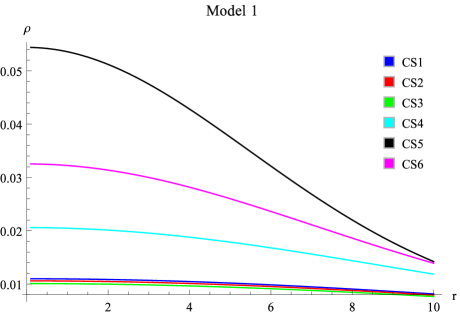
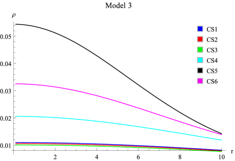
Figure 1: The density $(km^{-2})$ variation of strange compact stars candidate, $HerX-1$, $SAXJ1808.4-3658$, $4U1820-30$, $PSRJ16142230$, $VELAX-1$ and $CenX-3$ under three different viable Models.

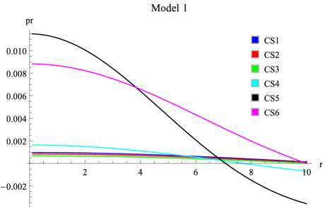
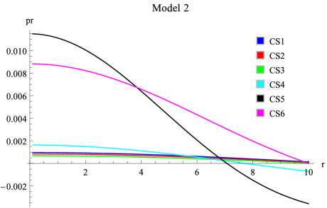
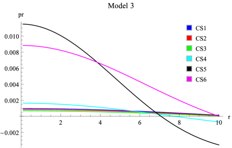
Figure 2: The radial pressure $(km^{-2})$ variation of strange compact stars candidate, $HerX-1$, $SAXJ1808.4-3658$, $4U1820-30$, $PSRJ16142230$, $VELAX-1$ and $CenX-3$ under three different viable Models.

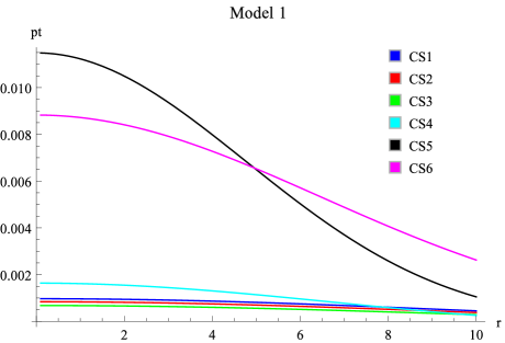
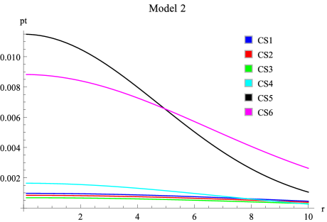
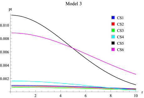
Figure 3: The transverse pressure $(km^{-2})$ variation of strange compact stars candidate, $HerX-1$, $SAXJ1808.4-3658$, $4U1820-30$, $PSRJ16142230$, $VELAX-1$ and $CenX-3$ under three different viable Models.

We deduced that, for all the six compact stars under three different viable models, $\frac{d\rho}{{dr}}<0$, $\frac{dp_{r}}{{dr}}<0$ and $\frac{dp_{t}}{{dr}}<0$. For $r\rightarrow 0$, we get

$$\frac{d\rho}{{dr}}\rightarrow 0$$

$$\frac{dp_{r}}{{dr}}\rightarrow 0$$

This is to be expected since these are diminishing functions, and we have a maximum density for small $r$ e.g. star core density $\rho_{c}=\rho(0)$.

3.2 Validity of Different Energy conditions

The Raychaudhuri equation for expansion [78] has been used to obtain the general structure of the energy conditions. The essence of gravity is appealing with positive energy density, which cannot flow faster than the speed of light, as can be deduced from these conditions. In Refs [79, 80, 81, 82, 83, 84], the terms ”Null-Energy conditions” $(NEC)$ and ”Strong-Energy conditions” $(SEC)$ are thoroughly discussed.

• WEC $:\Rrightarrow$ $\rho\geq 0$, ${\rho+p_{r}}\geq 0$, ${\rho+p_{t}}\geq 0$,

• NEC $:\Rrightarrow$ ${\rho+p_{r}}\geq 0$, ${\rho+p_{t}}\geq 0$,

• SEC $:\Rrightarrow$ ${\rho+p_{r}}\geq 0$, ${\rho+p_{t}}\geq 0$, ${\rho+p_{r}+2p_{t}}\geq 0$,

• DEC $:\Rrightarrow$ $\rho\geq|{p_{r}}|$, $\rho\geq|{p_{t}}|$.

All these energy conditions for the compact stars are fulfilled for our feasible models for all the six odd star candidates.

3.3 Tolman-Oppenheimer-Volkoff (TOV) Equation

The generalization of TOV equation can be written as

$$\frac{{d{p_{r}}}}{{dr}}+\frac{{a^{\prime}(p_{r}+\rho)}}{2}-\frac{{2({p_{t}}-{p_{r}})}}{r}=0$$ (20)

It can also be expressed in terms of magnetic, hydrostatic, and anisotropic forces

$$F_{h}+F_{g}+F_{a}=0,$$ (21)

which yields

$$F_{g}=-r(\rho+p_{r})B,F_{h}=-\frac{{d{p_{r}}}}{{dr}},F_{a}=-\frac{{2({p_{t}}-{p_{r}})}}{r}$$

We plot three different compact stars using these concepts, as seen in fig. (4)

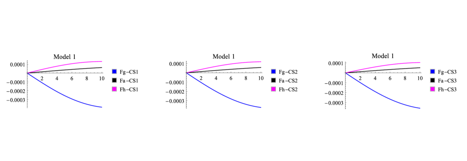
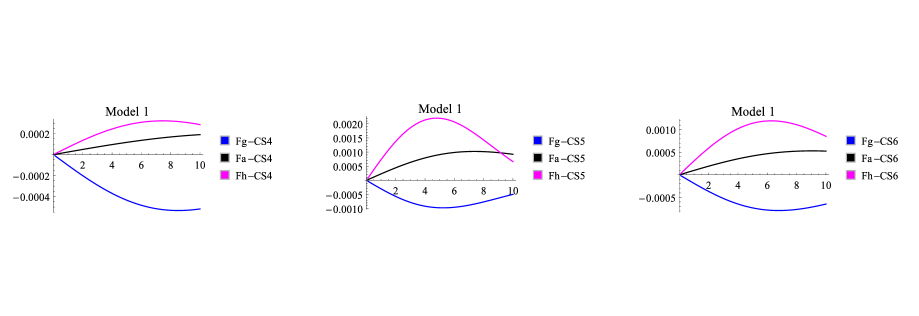
Figure 4: The variation of gravitational force ($F_{g}$), hydrostatic force ($F_{h}$) and anisotropic force $(F_{a})$ with respect to the radial coordinate r (km).

Concerning the radial coordinate $r(km)$, we can see the difference of gravitational force ($Fg$), hydrostatic force ($Fh$), and anisotropic force $(Fa)$. Model 1 is represented by the left plot, Model 2 by the middle plot, and Model 3 by the right plot.

3.4 The Stability-Scenario

Here, we look at the stability of compact star models under viable models in the $f(R,G)$ theory. To test our model’s stability, we measure the radial and transverse speeds as follows,

$$\frac{{d{p_{r}}}}{{d\rho}}=v_{sr}^{2}$$

and

$$\frac{{d{p_{t}}}}{{d\rho}}=v_{st}^{2}$$

For stability, the radial as well as the transverse speed should obey the condition $v_{sr}^{2}\in[0,1]$ and $v_{st}^{2}\in[0,1]$.

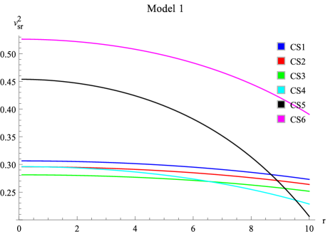
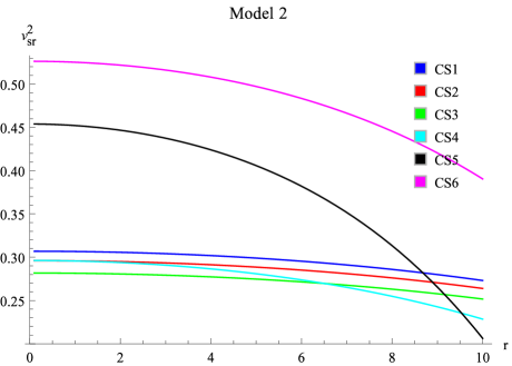
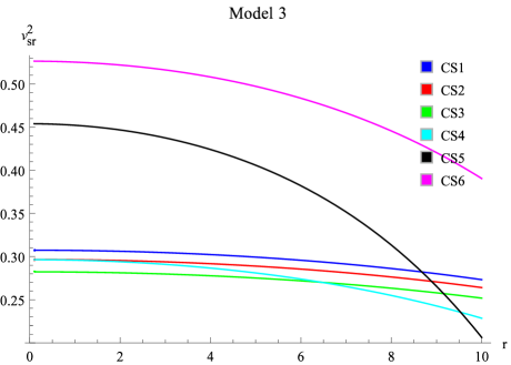
Figure 5: Variations of $v_{sr}^{2}$ with respect radius $r$ (km) of the strange stars

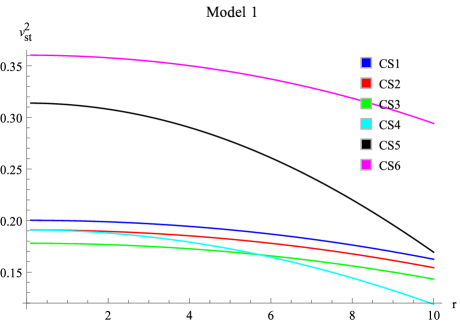
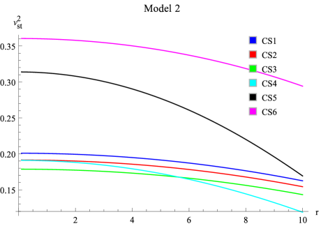
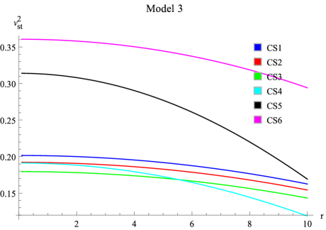
Figure 6: Variations of $v_{st}^{2}$ with respect radius $r$ (km) of the strange stars

It is evident from Figure (5) and (6), that the variations in radial and transversal sound speeds, for all the six types of odd star candidates, falls beyond the discussed stability bounds.

Similarly, we reached at

$$0<|v_{st}^{2}-v_{sr}^{2}|<1$$

so the stability is attained for compact stars in the $f(R,G)$ gravity models.

3.5 Equation of State Parameters

Now for the anisotropic case, the equation of state $(EoS)$ are written as

$$p_{r}=w_{r}\rho$$

and

$$p_{t}=w_{t}\rho.$$

For which the limits are like $0<w_{r}<1$ and $0<w_{t}<1$. The behavior of $w_{r}$ and $w_{t}$ are shown graphically in fig. (7) and (8) respectively.

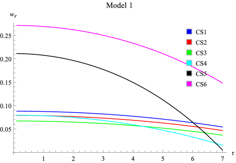
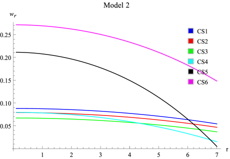
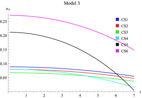
Figure 7: The variations of the radial EoS parameter against the radial coordinate, $r$ $(km)$.

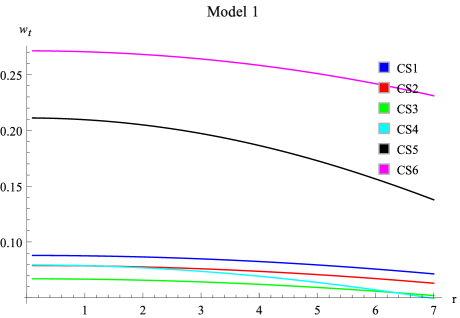
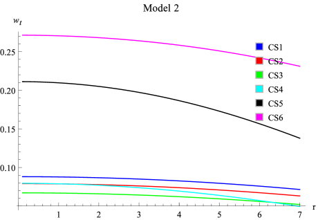
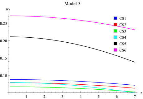
Figure 8: The variations of the transverse EoS parameter against the radial coordinate, $r$ $(km)$.

3.6 The Measurement of Anisotropy

The anisotropy is defined as

$$\Delta=\frac{2}{r}({p_{t}}-{p_{r}})$$ (22)

We get $\Delta>0$ while plotting the anisotropy, e.g. $p_{t}>p_{r}$, which indicates that the metric of anisotropy is oriented outward. Figure(9) illustrates these plots.

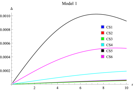
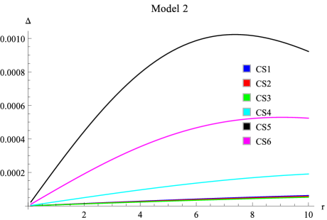
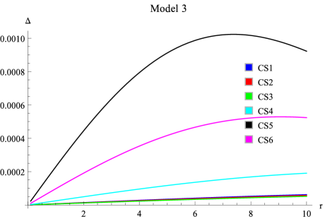
Figure 9: the variations of anisotropic measure $\Delta$ against the radial coordinate, $r$ $(km)$.

4 Summary

In this paper, we address the interior solution of compact stars by assuming that their internal structure is anisotropic in the modified gravity theory $f(R,G)$. In this respect, six compact stars, namely Her Stars $HerX-1$, $SAXJ1808.4-3658$, $4U1820-30$, $PSRJ16142230$, $VELAX-1$ and $CenX-3$ were considered to explore their physical features in the $f(R,G)$ theory of gravity. The arbitrary unknown constants $A$, $B$, and $C$ were extracted from the smooth matching condition of the Schwarzchild exterior-metric to the interior-metric’s analytic solutions. The matching condition enabled us to express the masses and radii of compact stars in terms of arbitrary constants and thus lead us to understand the nature and existence of these compact bodies. Based on their physical properties, the following conclusions about the anisotropic compact stars in the $f(R,G)$ gravity were drawn. Compact stars have the equation of state parameters that are the same as an ordinary-matter distribution in the $f(R,G)$ gravity, highlighting that they are made up of ordinary matter. The matter/energy density, as well as radial and tangential pressure, were plotted as a function of radial coordinate $r$ which revealed that for all the six strange star candidates the density reaches its maximum limit when $r$ goes to zero. It confirms that the compact star’s matter components are positive and finite in their interiors leading us to conclude that none of the six compact stars in this analysis have a singularity which further supports the theory that the cores of compact stars are extremely compact. The obtained results also verify as discussed in a recent proposed theory in Ref. [85]. It’s also worth noting that for $p_{t}<p_{r}$, the direction of anisotropic force is inward implying $\triangle<0$, while in the reverse scenario i.e., $p_{t}>p_{r}$ the anisotropy become positive suggesting that the anisotropic force is being outward-directed. For six distinct compact stars, the graphical representation of $\triangle>0$ is presented in fig $14$.

For each of the six compact stars under investigation, the TOV and energy conditions are examined as revealed in Fig. 5 and 6 respectively. Additionally, the inequality $|v^{2}_{sr}-v^{2}_{st}|<1$ holds for all the six candidates indicating that the models under consideration seems to be potentially stable in $f(R,G)$ gravity.

References

- [1] Kazuharu Bamba, Salvatore Capozziello, Shin’ichi Nojiri, and Sergei D Odintsov. Dark energy cosmology: the equivalent description via different theoretical models and cosmography tests. Astrophysics and Space Science, 342(1):155–228, 2012.
- [2] Hans A Buchdahl. Non-linear lagrangians and cosmological theory. Monthly Notices of the Royal Astronomical Society, 150(1):1–8, 1970.
- [3] Salvatore Capozziello, M De Laurentis, SD Odintsov, and A Stabile. Hydrostatic equilibrium and stellar structure in gravity. Physical Review D, 83(6):064004, 2011.
- [4] Sh Nojiri, SD Odintsov, and VK3683913 Oikonomou. Modified gravity theories on a nutshell: inflation, bounce and late-time evolution. Physics Reports, 692:1–104, 2017.
- [5] Salvatore Capozziello and Mariafelicia De Laurentis. Extended theories of gravity. Physics Reports, 509(4-5):167–321, 2011.
- [6] Shin’ichi Nojiri and Sergei D Odintsov. Unified cosmic history in modified gravity: from theory to lorentz non-invariant models. Physics Reports, 505(2-4):59–144, 2011.
- [7] Tiberiu Harko and Francisco SN Lobo. Two-fluid dark matter models. Physical Review D, 83(12):124051, 2011.
- [8] Zhen Zhang. Geometrization of light bending and its application to sds w spacetime. Classical and Quantum Gravity, 39(1):015003, 2021.
- [9] David Lovelock. The einstein tensor and its generalizations. Journal of Mathematical Physics, 12(3):498–501, 1971.
- [10] Guido Cognola, Emilio Elizalde, Shin’ichi Nojiri, Sergei D Odintsov, and Sergio Zerbini. Dark energy in modified gauss-bonnet gravity: Late-time acceleration and the hierarchy problem. Physical Review D, 73(8):084007, 2006.
- [11] Emilio Elizalde, Ratbay Myrzakulov, Valery V Obukhov, and Diego Sáez-Gómez. cdm epoch reconstruction from and modified gauss–bonnet gravities. Classical and Quantum Gravity, 27(9):095007, 2010.
- [12] VK Oikonomou and FP Fronimos. A nearly massless graviton in einstein-gauss-bonnet inflation with linear coupling implies constant-roll for the scalar field. EPL (Europhysics Letters), 131(3):30001, 2020.
- [13] VK Oikonomou. A refined einstein–gauss–bonnet inflationary theoretical framework. Classical and Quantum Gravity, 38(19):195025, 2021.
- [14] Sergei D Odintsov, VK Oikonomou, and FP Fronimos. Rectifying einstein-gauss-bonnet inflation in view of gw170817. Nuclear Physics B, 958:115135, 2020.
- [15] VK Oikonomou. Singular bouncing cosmology from gauss-bonnet modified gravity. Physical Review D, 92(12):124027, 2015.
- [16] Shin’ichi Nojiri and Sergei D Odintsov. Modified gravity consistent with realistic cosmology: From a matter dominated epoch to a dark energy universe. Physical Review D, 74(8):086005, 2006.
- [17] Shin’ichi Nojiri and Sergei D Odintsov. Modified gauss–bonnet theory as gravitational alternative for dark energy. Physics Letters B, 631(1-2):1–6, 2005.
- [18] J Santos, JS Alcaniz, and MJ Rebouças. Energy conditions and supernovae observations. Physical Review D, 74(6):067301, 2006.
- [19] J Santos, JS Alcaniz, N Pires, and Marcelo J Reboucas. Energy conditions and cosmic acceleration. Physical Review D, 75(8):083523, 2007.
- [20] M Farasat Shamir and Mushtaq Ahmad. Noether symmetry approach in gravity. The European Physical Journal C, 77(1):1–6, 2017.
- [21] M Farasat Shamir and Mushtaq Ahmad. Some exact solutions in gravity via noether symmetries. Modern Physics Letters A, 32(16):1750086, 2017.
- [22] M Sharif and Ayesha Ikram. Stability analysis of some reconstructed cosmological models in gravity. Physics of the dark universe, 17:1–9, 2017.
- [23] M Sharif and Ayesha Ikram. Stability analysis of einstein universe in gravity. International Journal of Modern Physics D, 26(08):1750084, 2017.
- [24] Albert Einstein. Auf die riemann-metrik und den fern-parallelismus gegründete einheitliche feldtheorie. Mathematische Annalen, 102(1):685–697, 1930.
- [25] Kenji Hayashi and Takeshi Shirafuji. New general relativity. Physical Review D, 19(12):3524, 1979.
- [26] Yi-Fu Cai, Salvatore Capozziello, Mariafelicia De Laurentis, and Emmanuel N Saridakis. teleparallel gravity and cosmology. Reports on Progress in Physics, 79(10):106901, 2016.
- [27] Christian G Boehmer, Atifah Mussa, and Nicola Tamanini. Existence of relativistic stars in gravity. Classical and Quantum Gravity, 28(24):245020, 2011.
- [28] Baojiu Li, John D Barrow, and David F Mota. Cosmology of modified gauss-bonnet gravity. Physical Review D, 76(4):044027, 2007.
- [29] James M Lattimer and Andrew W Steiner. Neutron star masses and radii from quiescent low-mass X-ray binaries. The Astrophysical Journal, 784(2):123, 2014.
- [30] TR Jaffe, AJ Banday, JP Leahy, S Leach, and AW Strong. Connecting synchrotron, cosmic rays and magnetic fields in the plane of the galaxy. Monthly Notices of the Royal Astronomical Society, 416(2):1152–1162, 2011.
- [31] Antonio De Felice and Shinji Tsujikawa. Construction of cosmologically viable gravity models. Physics Letters B, 675(1):1–8, 2009.
- [32] M Alimohammadi and A Ghalee. Remarks on generalized gauss-bonnet dark energy. Physical Review D, 79(6):063006, 2009.
- [33] Christian G Boehmer and Francisco SN Lobo. Stability of the einstein static universe in modified gauss-bonnet gravity. Physical Review D, 79(6):067504, 2009.
- [34] Kotub Uddin, James E Lidsey, and Reza Tavakol. Cosmological scaling solutions in generalised gauss–bonnet gravity theories. General Relativity and Gravitation, 41(12):2725–2736, 2009.
- [35] Shuang-Yong Zhou, Edmund J Copeland, and Paul M Saffin. Cosmological constraints on dark energy models. Journal of Cosmology and Astroparticle Physics, 2009(07):009, 2009.
- [36] S Nojiri, SD Odintsov, VK Oikonomou, and Arkady A Popov. Ghost-free gravity. Nuclear Physics B, 973, 2021.
- [37] Mariafelicia De Laurentis, Mariacristina Paolella, and Salvatore Capozziello. Cosmological inflation in gravity. Physical Review D, 91(8):083531, 2015.
- [38] Salvatore Capozziello, Mariafelicia De Laurentis, and Sergei D Odintsov. Noether symmetry approach in gauss–bonnet cosmology. Modern Physics Letters A, 29(30):1450164, 2014.
- [39] K Atazadeh and F Darabi. Energy conditions in gravity. General Relativity and Gravitation, 46(2):1–14, 2014.
- [40] Naureen Goheer, Rituparno Goswami, Peter KS Dunsby, and Kishore Ananda. Coexistence of matter dominated and accelerating solutions in gravity. Physical Review D, 79(12):121301, 2009.
- [41] M Farasat Shamir and Saeeda Zia. Gravastars in gravity. Canadian Journal of Physics, 98(9):849–852, 2020.
- [42] Shin’ichi Nojiri and Sergei D Odintsov. Introduction to modified gravity and gravitational alternative for dark energy. International Journal of Geometric Methods in Modern Physics, 4(01):115–145, 2007.
- [43] CW Misner, KS Thorne, and JA Wheeler. Review of publications-gravitation. Journal of the Royal Astronomical Society of Canada, 68:164, 1974.
- [44] Takeshi Chiba. Generalized gravity and a ghost. Journal of Cosmology and Astroparticle Physics, 2005(03):008, 2005.
- [45] Savaş Arapoğlu, Cemsinan Deliduman, and K Yavuz Ekşi. Constraints on perturbative gravity via neutron stars. Journal of Cosmology and Astroparticle Physics, 2011(07):020, 2011.
- [46] Artyom V Astashenok, Salvatore Capozziello, and Sergei D Odintsov. Maximal neutron star mass and the resolution of the hyperon puzzle in modified gravity. Physical Review D, 89(10):103509, 2014.
- [47] H Rizwana Kausar and Ifra Noureen. Dissipative spherical collapse of charged anisotropic fluid in gravity. The European Physical Journal C, 74(2):1–8, 2014.
- [48] G Abbas, Sumara Nazeer, and MA Meraj. Cylindrically symmetric models of anisotropic compact stars. Astrophysics and Space Science, 354(2):449–455, 2014.
- [49] G Abbas, M Zubair, and G Mustafa. Anisotropic strange quintessence stars in gravity. Astrophysics and Space Science, 358(2):1–11, 2015.
- [50] G Abbas, S Qaisar, Wajiha Javed, and MA Meraj. Compact stars of emending class one in gravity. Iranian Journal of Science and Technology, Transactions A: Science, 42(3):1659–1668, 2018.
- [51] Artyom V Astashenok, Salvatore Capozziello, and Sergei D Odintsov. Further stable neutron star models from gravity. Journal of Cosmology and Astroparticle Physics, 2013(12):040, 2013.
- [52] Artyom V Astashenok, Salvatore Capozziello, and Sergei D Odintsov. Extreme neutron stars from extended theories of gravity. Journal of Cosmology and Astroparticle Physics, 2015(01):001, 2015.
- [53] Kalin V Staykov, Daniela D Doneva, and Stoytcho S Yazadjiev. Orbital and epicyclic frequencies around neutron and strange stars in gravity. The European Physical Journal C, 75(12):1–7, 2015.
- [54] Salvatore Capozziello, Mariafelicia De Laurentis, Ruben Farinelli, and Sergei D Odintsov. Mass-radius relation for neutron stars in gravity. Physical Review D, 93(2):023501, 2016.
- [55] M Ilyas, AR Athar, and Bilal Masud. Relativistic charged sphere in gravity. International Journal of Geometric Methods in Modern Physics, 18(10):2150152, 2021.
- [56] M Ilyas. Compact stars with variable cosmological constant in gravity. Astrophysics and Space Science, 365(11):1–11, 2020.
- [57] M. Ilyas. Charged compact stars in gravity. The European Physical Journal C, 78(9):1–12, 2018.
- [58] Z. Yousaf, M. Zaeem-ul-Haq Bhatti, and M. Ilyas. Existence of compact structures in gravity. Eur. Phys. J. C, 78(4):307, 2018.
- [59] M. Ilyas, Z. Yousaf, M. Z. Bhatti, and Bilal Masud. Existence of relativistic structures in gravity. Astrophys. Space Sci., 362(12):237, 2017.
- [60] Z. Yousaf, M. Sharif, M. Ilyas, and M. Z. Bhatti. Influence of models on the existence of anisotropic self-gravitating systems. Eur. Phys. J. C, 77(10):691, 2017.
- [61] M. Z. Bhatti, Z. Yousaf, and M. Ilyas. Evolution of Compact Stars and Dark Dynamical Variables. Eur. Phys. J. C, 77(10):690, 2017.
- [62] Muhammad Zaeem-ul-Haq Bhatti, M. Sharif, Z. Yousaf, and M. Ilyas. Role of gravity on the evolution of relativistic stars. Int. J. Mod. Phys. D, 27(04):1850044, 2017.
- [63] Stoytcho S Yazadjiev, Daniela D Doneva, and Kostas D Kokkotas. Rapidly rotating neutron stars in R-squared gravity. Physical Review D, 91(8):084018, 2015.
- [64] Kalin V Staykov, Daniela D Doneva, Stoytcho S Yazadjiev, and Kostas D Kokkotas. Slowly rotating neutron and strange stars in gravity. Journal of Cosmology and Astroparticle Physics, 2014(10):006, 2014.
- [65] AV Astashenok, Salvatore Capozziello, Sergei D Odintsov, and Vasilis K Oikonomou. Maximum baryon masses for static neutron stars in gravity. Europhysics Letters, 136(5):59001, 2022.
- [66] AV Astashenok, Salvatore Capozziello, Sergei D Odintsov, and VK4234883 Oikonomou. Causal limit of neutron star maximum mass in gravity in view of gw190814. Physics Letters B, 816:136222, 2021.
- [67] Artyom V Astashenok, Salvatore Capozziello, Sergei D Odintsov, and Vasilis K Oikonomou. Extended gravity description for the gw190814 supermassive neutron star. Physics Letters B, 811:135910, 2020.
- [68] AV Astashenok, Salvatore Capozziello, Sergei D Odintsov, and VK Oikonomou. Novel stellar astrophysics from extended gravity. EPL (Europhysics Letters), 134(5):59001, 2021.
- [69] VK Oikonomou. Universal inflationary attractors implications on static neutron stars. Classical and Quantum Gravity, 38(17):175005, 2021.
- [70] SD Odintsov and VK Oikonomou. Neutron stars in scalar-tensor gravity with higgs scalar potential. arXiv preprint arXiv:2104.01982, 2021.
- [71] Sergei D Odintsov and VK Oikonomou. Neutron stars phenomenology with scalar–tensor inflationary attractors. Physics of the Dark Universe, 32:100805, 2021.
- [72] MK Mak, Peter N Dobson Jr, and T Harko. Maximum mass–radius ratio for compact general relativistic objects in schwarzschild–de sitter geometry. Modern Physics Letters A, 15(35):2153–2158, 2000.
- [73] Dimitrios Psaltis. Probes and tests of strong-field gravity with observations in the electromagnetic spectrum. Living Reviews in Relativity, 11(1):1–61, 2008.
- [74] Shinji Tsujikawa. Observational signatures of dark energy models that satisfy cosmological and local gravity constraints. Physical Review D, 77(2):023507, 2008.
- [75] Hans-Jürgen Schmidt. Gauss-bonnet lagrangian and cosmological exact solutions. Physical Review D, 83(8):083513, 2011.
- [76] Kazuharu Bamba, Sergei D Odintsov, Lorenzo Sebastiani, and Sergio Zerbini. Finite-time future singularities in modified gauss–bonnet and gravity and singularity avoidance. The European Physical Journal C, 67(1):295–310, 2010.
- [77] Shin’ichi Nojiri, Sergei D Odintsov, and Petr V Tretyakov. From inflation to dark energy in the non-minimal modified gravity. Progress of Theoretical Physics Supplement, 172:81–89, 2008.
- [78] Stephen W Hawking and George Francis Rayner Ellis. The large scale structure of space-time, volume 1. Cambridge university press, 1973.
- [79] J Santos, JS Alcaniz, MJ Reboucas, and FC Carvalho. Energy conditions in gravity. Physical Review D, 76(8):083513, 2007.
- [80] Leonardo Balart and Elias C Vagenas. Regular black hole metrics and the weak energy condition. Physics Letters B, 730:14–17, 2014.
- [81] Matt Visser. Energy conditions in the epoch of galaxy formation. Science, 276(5309):88–90, 1997.
- [82] Nadiezhda M García, Francisco SN Lobo, José P Mimoso, and Tiberiu Harko. modified gravity and the energy conditions. In Journal of Physics: Conference Series, volume 314, page 012056. IOP Publishing, 2011.
- [83] K Atazadeh and F Darabi. Energy conditions in gravity. General Relativity and Gravitation, 46(2):1–14, 2014.
- [84] Orfeu Bertolami and Miguel Carvalho Sequeira. Energy conditions and stability in theories of gravity with nonminimal coupling to matter. Physical Review D, 79(10):104010, 2009.
- [85] M Ilyas. Compact stars in gravity. International Journal of Modern Physics A, 36(24):2150165, 2021.