Example Perplexity

Abstract

Some examples are easier for humans to classify than others. The same should be true for deep neural networks (DNNs). We use the term example perplexity to refer to the level of difficulty of classifying an example. In this paper, we propose a method to measure the perplexity of an example and investigate what factors contribute to high example perplexity. The related codes and resources are available at https://github.com/vaynexie/Example-Perplexity.

1 Introduction

Some examples are easier for humans to classify than others. The same should be true for deep neural networks (DNNs). We use the term example perplexity to refer to the level of difficulty of classifying an example. While scarce, there are previous works that consider classification difficulty of examples and datasets. Ionescu et al. [7] estimate image difficulty by learning a regression model from human-originated scores, which are converted from response times during visual search tasks. Yu et al. [8] view disagreement among experts when labeling medical images as an indication of their difficulty. Both of those two methods rely on human annotations and hence do not scale up. Scheidegger et al. [5] use the average performance of top models as a measure of the difficulty of a dataset. Li et al.[3] and Nie et al. [4] exploit pixel difficulty in the context of semantic segmentation. Those two methods are not about example difficulty.

In this paper, we propose a method to measure the perplexity of an example and investigate what factors contribute to high example perplexity. To estimate the perplexity of an image for DNNs, we create a population of DNN classifiers with varying architectures and trained on data of varying sample sizes, just as different people have different IQs and different amounts of experiences. For an unlabeled example, the average entropy of the output probability distributions of the classifiers is taken to be the C-perplexity of the example, where C stands for “confusion”. For a labeled example, the fraction of classifiers that misclassify the example is taken to be the X-perplexity of the example, where X stands for “mistake”.

Perplexity analysis on the examples from ImageNet has revealed several interesting. In particular, some insights are gained regarding what makes some images harder to classify than others. It is also found that perplexity analysis can reveal imperfections of a dataset, which can potentially help with data cleaning

While we use a large population of classifiers consisting of both strong and week models to measure example perplexity, Tsipras et al. [6] and Beyer et al. [1] use a small population of state-of-the-art classifiers to suggest candidate labels for images for the purpose of data quality improvement.

2 C-Perplexity and X-Perplexity

An image is difficult to classify for humans if many people find it confusing and classify it incorrectly. Motivated by this observation, we measure example perplexity in reference to a population classifiers. Let ${\cal C}$ be a population of $N$ classifiers for classifying examples into $M$ classes. For a given example ${\bf x}$, $P_{i}(y|{\bf x})$ is the probability distribution over the $M$ classes computed by classifier $i$. The entropy $H(P_{i}(y|{\bf x}))=-\sum_{y}P_{i}(y|{\bf x})\log_{2}P_{i}(y|{\bf x})$ is a measure of how uncertain the classifier is when classifying ${\bf x}$. The perplexity of the probability distribution is defined to be $2^{H(P_{i}(y|{\bf x}))}$ . The larger the perplexity, the less confident the classifier is about its prediction. When the distribution places equal probability on $k$ possible classes and zero probability on others, the perplexity is $k$.

We define the C-perplexity of an unlabelled example ${\bf x}$ w.r.t ${\cal C}$ to be the following geometric mean:

$$\Phi_{C}({\bf x})=[\prod_{i=1}^{N}2^{H(P_{i}(y|{\bf x}))}]^{\frac{1}{N}}.$$

The prefix “C” stands for “confusion”. The minimum possible value of C-perplexity is 1. High C-perplexity value indicates that the classifiers have low confidence when classifying the example.

We define the X-perplexity of an labelled example $({\bf x},y)$ w.r.t ${\cal C}$ to be

$$\Phi_{X}({\bf x})=\frac{1}{N}\sum_{i=1}^{N}{\bf 1}(C_{i}({\bf x})\neq y),$$

where $C_{i}({\bf x})=\arg\max_{y}P_{i}(y|{\bf x})$ is the class assignment function, and ${\bf 1}$ is the indicator function. In words, it is the fraction of the classifiers that misclassifies the example, hence is between 0 and 1. The prefix “X” stands for “misclassification”.

3 Creation of a Classifier Population

We have created a population of 500 classifiers of varying strengths. We started with 10 popular model architectures (Table 1) designed for the ImageNet dataset, which consists of approximately 14 million training examples. Besides the original ImageNet training set, we created 9 smaller training sets via sub-sampling without replacement. They are evenly divided into three groups, with 25%, 50% and 75% of the training examples respectively. We trained each of the 10 architectures on each of 10 training sets. During each training session, four models were collected at different epochs prior and close to convergence, and one model was collected at convergence.

Table 1: Seed model architectures for our classifier population.

Structure	# Parameters (M)	Storage Space (MB)
VGG16	138	500
ResNet50	25	98
ResNet101	44	171
InceptionV3	24	92
Xception	23	88
DenseNet121	8	33
DenseNet169	14	57
DenseNet201	20	80
EfficientNetB0	5.3	20
EfficientNetB2	9	36

Generally speaking, classifiers trained with less data and for fewer epochs are weaker than those trained with more data and for more epochs. Why do we need weak classifiers in addition to strong ones? This question can be answered by making an analogy to educational testing, where a key concern is to design test items with appropriate difficult levels. To determine the difficult level of a particular item, responses from a population of students need to be collected and analyzed using item response theory [2]. It is evident that one cannot properly determine the difficult level of a test item by trying it only on strong students. Similarly, we need classifiers of varying strengths to properly determine the classification difficulty of an image. Architectures with different complexity can be compared to students with different IQs. Different training sets with various sample sizes can be compared to different experiences students have access to. Different training epochs can be compared to how much students digest their experiences.

Note that, while ensemble learning involves multiple classifiers that are complementary in strength, we need multiple classifiers with a variety of strengths in this project.

4 Perplexity Analysis of the ImageNet DataSet

Based on the aforementioned 500 classifiers, we have computed the C-perplexity and X-perplexity of the 50,000 images in the validation set of ImageNet. Figure 1 shows several examples with C-perplexity values ranging from 1 to 15, and Figure 2 shows several examples with x-perplexity values ranging from 0 to 1. In Section 5, we will analyze the factors that contribute to high perplexity.

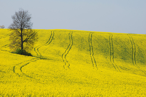
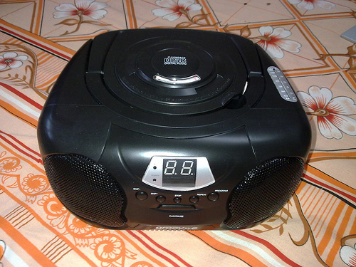
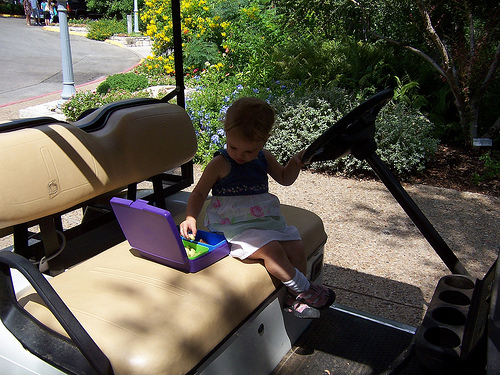
Label = rapeseed	Label = CD player	Label = golfcart
CP = 1	CP =2	CP =3
XP = 0	XP =0.15	XP =0.29
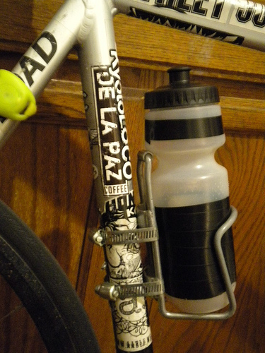
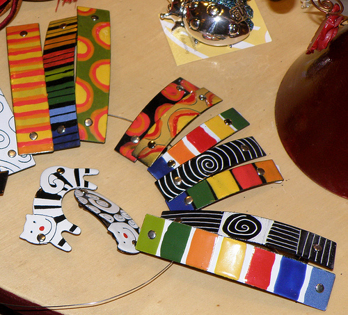
Label = water bottle	Label = match stick	Label = hair slide
CP = 5	CP = 10	CP =15
XP = 0.74	XP =0.99	XP =0.99

Figure 1: Examples with varying C-perplexity values.

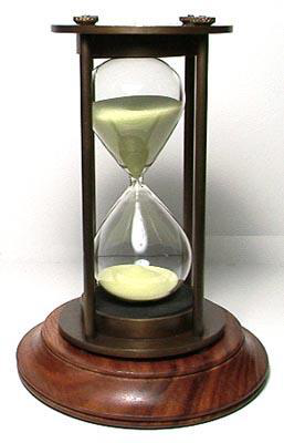
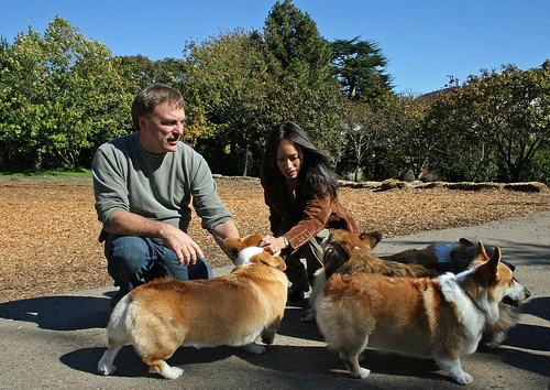
Label = hourglass	Label = stone wall	Label = mousetrap
XP = 0	XP =0.2	XP =0.4
CP = 1	CP =1.14	CP =8.07
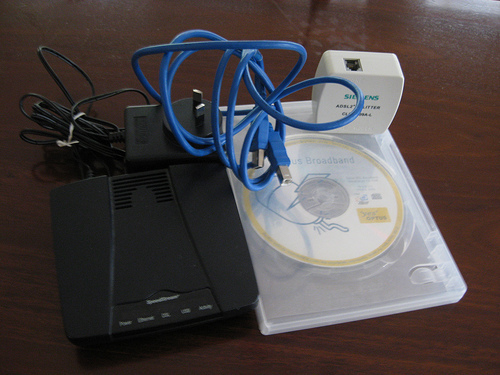
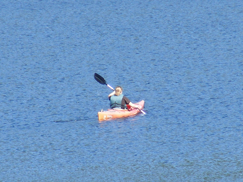
Label = modem	Label = paddle	Label = oil filter
XP = 0.6	XP =0.8	XP =1.0
CP = 4.37	CP = 10.9	CP =14.7

Figure 2: Examples with varying X-perplexity values.

Figure 3 shows the distribution of the examples over the C-perplexity values. As mentioned earlier, a C-perplexity value of $k$ amounts to the uncertainty of choosing among $k$ equally probable classes. The distribution indicates that, in most cases, the classifiers can narrow down the number of possible classes to small numbers. However, there are 5 images with C-perplexity larger than 30. One example is given in the figure.

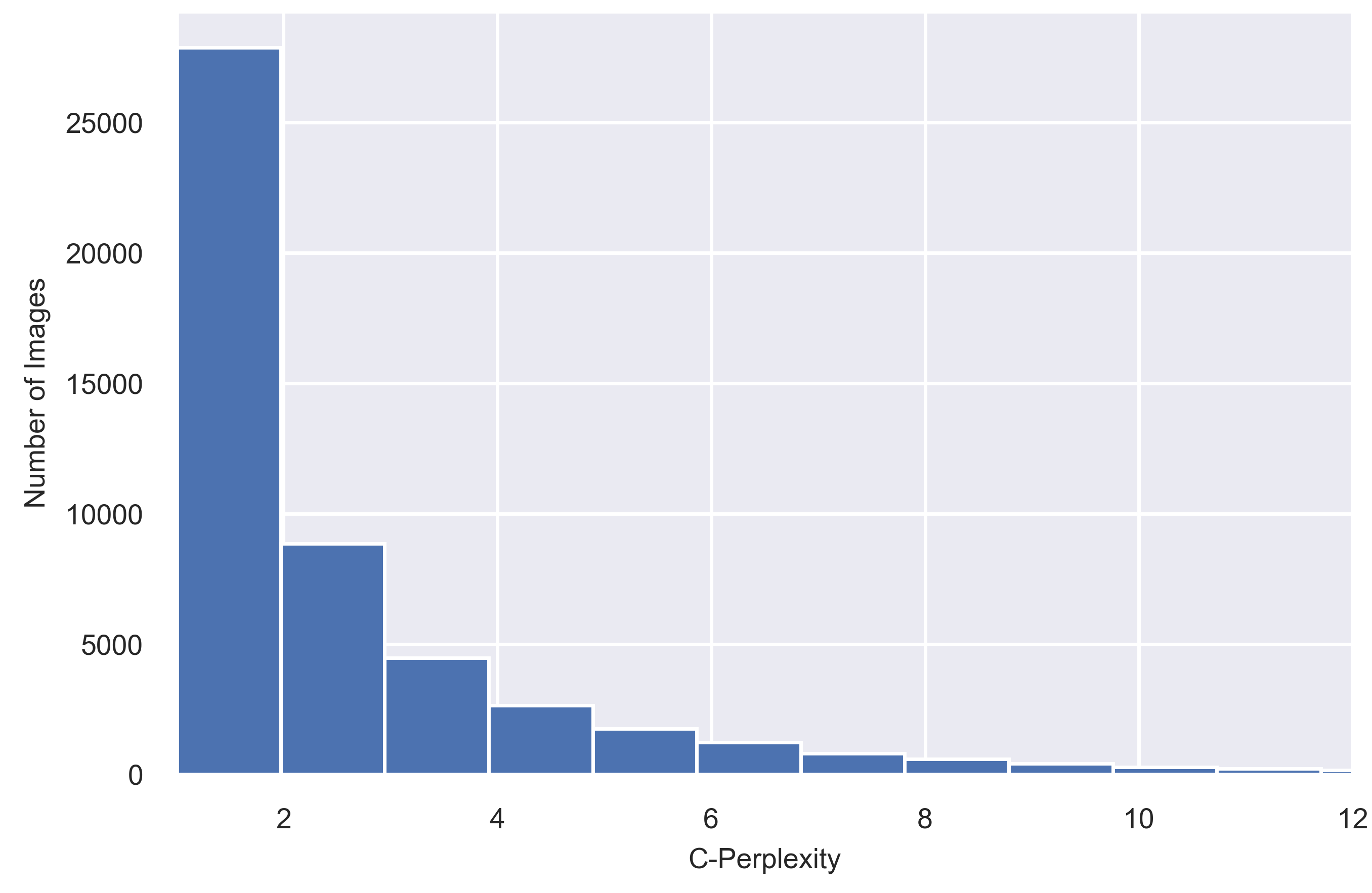
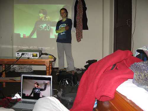
Label = home theatre

Figure 3: Distribution of examples over C-perplexity values (left), and one image with C-Perplexity value larger than 30 (right).

Figure 4 shows the distribution of the example over the X-perplexity values. It is interesting to observe that the curve is U-shaped. This means that, while the majority of the examples are easy to classify, many of them are difficult for most and even all the classifiers. There are two reasons: First, some images are genuinely confusing to the classifiers (Section 5). Second, some images are incorrectly or inappropriately labeled in the ImageNet dataset (Section 7). The two reasons will be analyzed in details later in this paper.

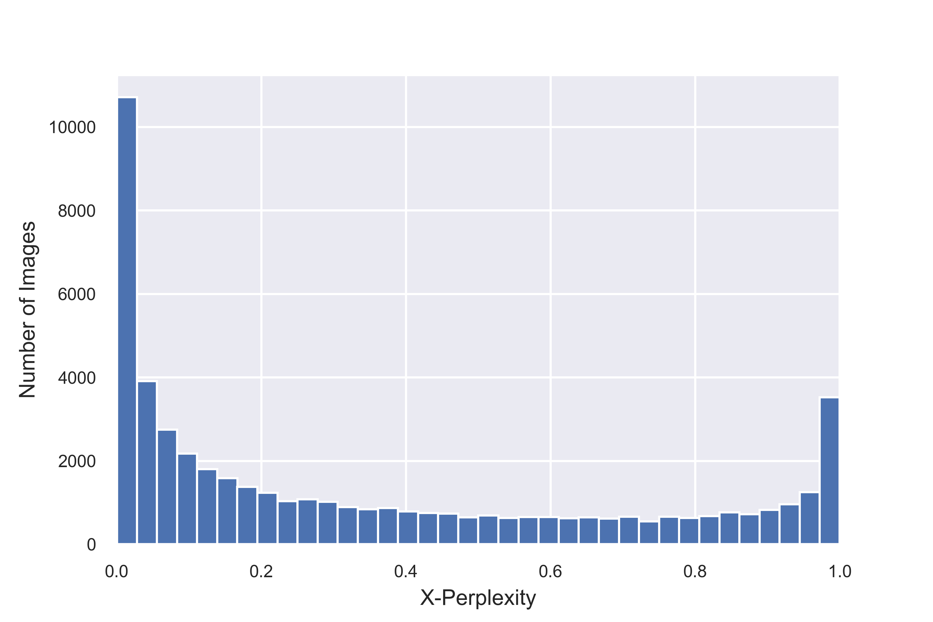
Figure 4: Distribution of examples over X-perplexity values.

C-perplexity and X-perplexity are strongly correlated. They are both influenced by the population of classifiers that is used in the computation. Detailed discussions of those issues can be found in Appendices 1 and 2 respectively.

5 What Makes an Image Difficult to Classify?

There are multiple factors that make an image difficult to classify, for example, clutter, occlusions, and adversarial perturbations. An inspection of examples with high perplexity reveals two other conceptually interesting reasons that we will exploit later in this project. The first one is attention confusion, which refers to the difficulty that a classifier faces, when classifying an image with multiple objects, in deciding which object to place attention on. The second one is class confusion, which refers to the difficulty that a classifier faces in deciding, among multiple visually similar classes, which class an object belongs to. The two concepts are illustrated in Figure 5.

In the case of attention confusion, a classifier is uncertain about which object to focus on and hence outputs significant probabilities for multiple class labels, with different labels corresponding to different regions of the image. This leads to high C-perplexity. In addition, no matter which class is designated as the label of the image, some classifiers will assign the image to other competing classes, resulting in high X-perplexity. In the case of class confusion, a classifier typically outputs significant probabilities for multiple visually similar classes, leading to high C-perplexity. In addition, classifiers might assign the image to the wrong classes, resulting in high X-perplexity.

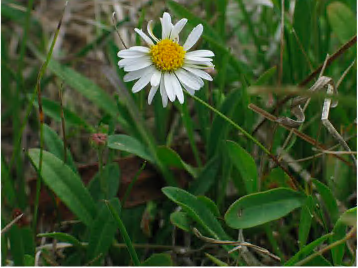
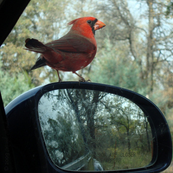
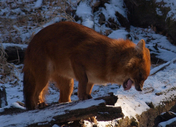
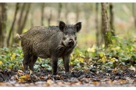
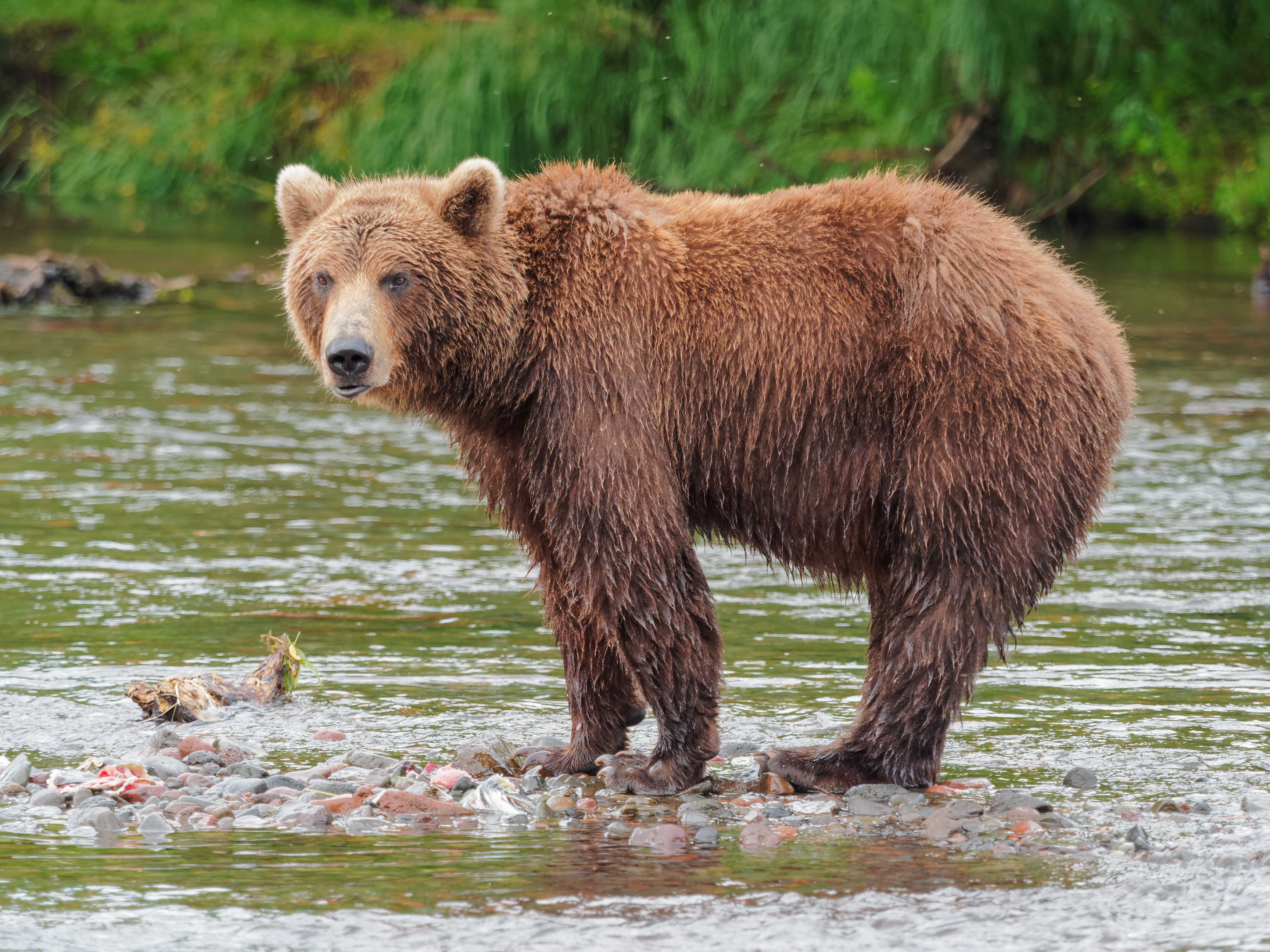
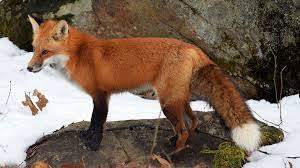
(a) Low perplexity (b) Attention confusion True label: Dhole Similar class: Wild boar Similar class: Brown bear Similar class: Red fox (c) Class confusion

Figure 5: Attention confusion and class confusion. (a): There is one main object in the image and it is visually distinct. Both the C-perplexity (1.26) and the X-perplexity (0.04) are low. (b): There are multiple (two) main objects, which causes attention confusion. The C-perplexity (1.77 ) and the X-perplexity (0.8) are higher than in the previous case. (c): There is one main object. However, it visually resembles objects from several other classes. This leads to class confusion. The C-perplexity (2.3) and the X-perplexity (0.25) are higher than in the case of (a).

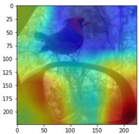
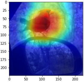
Original	Car mirror	House flinch

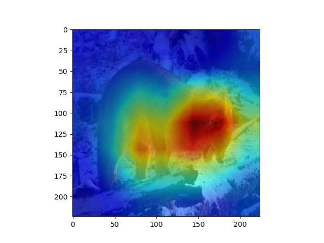
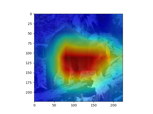
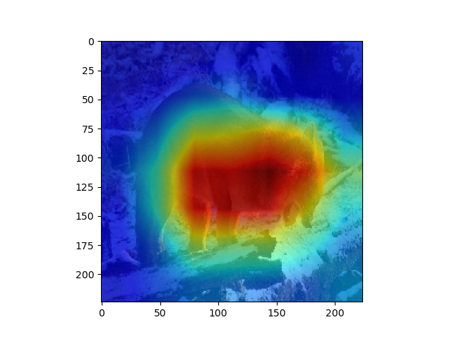
Original	Dhole	Brown bear	Wild boar

Figure 6: Grad-Cam heatmaps based on the best ResNet50 model. Top row: The classifier focuses at different regions of the image for different classes. The difficulty is to decide which part to focus on. Bottom row: The classifier focuses on the same region for different classes. The difficulty is to decide what the object is.

How do we know if attention confusion and/or class confusion play an role in the classification of an example? To answer this question, we need to introduce two concepts. The fraction of the classifiers that classify an example ${\bf x}$ into a class $j$ is:

$$f({\bf x},j)=\frac{1}{N}\sum_{i=1}^{N}{\bf 1}(C_{i}({\bf x})=j).$$

It can also be viewed as the fraction of the votes that ${\bf x}$ receives from the classifiers. We call the class labels with the highest numbers of the votes the top voted labels of ${\bf x}$.

The probability that ${\bf x}$ belongs to class $j$ according to classifier $i$ is $P_{i}(j|{\bf x})$. Imagine assigning ${\bf x}$ to a class via sampling according to $P_{i}(j|{\bf x})$ rather than to assign it to the class with the maximum probability. Then the expected number of classifiers that assign ${\bf x}$ to class $j$ would be:

$$f_{e}({\bf x},j)=\frac{1}{N}\sum_{i=1}^{N}P_{i}(j|{\bf x}).$$

It can also be viewed as the expected fraction of the votes that ${\bf x}$ receives from the classifiers. We call the class labels with the highest expected number votes the top expected labels of ${\bf x}$.

The top voted labels for the image in Figure 5 (b) are car mirror and house flinch. The top expected labels are the same. Apparently, those class labels correspond to different regions of the image (Figure 6, tope row). Therefore, we know that attention confusion is what makes the image difficult to classify for the classifiers.

For the image in Figure 5 (c) (top-right), the top 3 voted labels are dhole, brown bear and wild boar. The top 3 expected labels are dhole, brown bear and red fox. All those classes are visually similar, and are referring to the same object in the image (Figure 6, bottom row). Therefore, we know that class confusion is what makes the image difficult to classify for the classifiers.

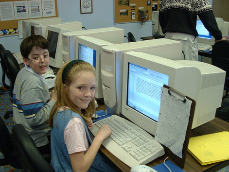
Figure 7: Mixed confusion. The C-perplexity (5.7) and the X-perplexity (0.86) are both high.

Often, a classifier must confront both attention confusion and class confusion. One example is shown in Figure 7. The ground truth label of the image is screen. In the results of ResNet50, the five classes with the highest probability values are: laptop (0.58), notebook (0.13), crossword puzzle (0.07), desk (0.06), desktop computer (0.03). They can be divided into three groups: (1) laptop, notebook, desktop computer; (2) crossword puzzle; and (3) desk. The difficulty in distinguishing between classes in the first group is due to class confusion, and the difficulty in distinguishing between different groups is due to attention confusion.

6 Class Perplexity

The validation set of ImageNet consists of 1,000 classes, each with 50 images. In the previous section, we have discussed perplexity of individual examples. In this section, we extend the concept to classes. Specifically, the C/X-perplexity of a class is defined to be the average of the C/X-perplexity values of all the examples in the class. The classes with the highest C-perplexity and X-perplexity are given in Table 2 .

Table 2: Classes with the highest C-perplexity and X-perplexity.

Class	C-perplexity	Class	X-perplexity
screwdriver	7.78	velvet	0.87
loupe	7.04	screen	0.85
miniskirt	6.73	sunglass	0.81
sunglasses	6.48	water jug	0.80
hair spray	6.17	hook	0.77
hatchet	6.15	spotlight	0.77
power drill	6.10	ladle	0.76
backpack	5.99	English foxhound	0.75
sunglass	5.77	laptop	0.75
plunger	5.61	chiffonier	0.75

What factors contribute to high class perplexity? In other words, what makes a class difficulty to classify? To answer this question, we need to introduce some new concepts for classes.

As defined in the previous section, $f({\bf x},j)$ denotes the fraction of the votes that the example ${\bf x}$ receives from the classifiers. For a given class $c$, let $f(c,j)$ be the average of $f({\bf x},j)$ over all the examples in the class. It is the frequency that class $c$ is confused as class $j$. Note that $f(c,j)\neq f(j,c)$ in general.

Define the voted-confusion between the two classes to be $s(c,j)=\frac{f(c,j)+f(j,c)}{2}$. We refer to the class labels $j$ with highest $f(c,j)$ as the top voted-confusion labels of class $c$. In a similar fashion, we define expected-confusion between classes and top expected-confusion labels of a class.

An inspection of pairs of top confusion classes reveals that two factors make a class difficult to classifier. The first factor is visual similarity between classes. Take English foxhound as an example. It has high voted-confusion with Walker hound and beagle. Examples of the three classes from ImageNet are shown in Figure 8. It is clear that the three classes do look very similar.

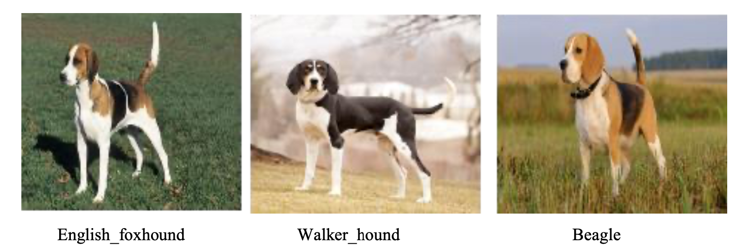
Figure 8: Example images of the classes English foxhound, Walker hound and beagle from ImageNet. The three classes have high voted-confusion.

The screwdriver class has high expected-confusion with springe and paintbrush. Examples of the three classes from ImageNet are shown in Figure 9. Although they might look very different for humans, they are actually very similar to the classifiers.

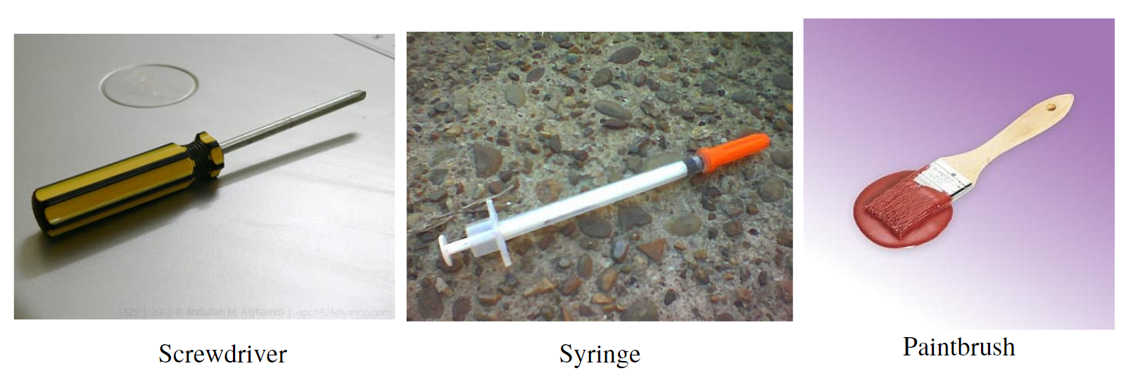
Figure 9: Example images of the classes screwdriver, syringe and paintbrush from ImageNet. The three classes have high expected-confusion.

The second reason for high class perplexity is class co-occurence. For example, the screen class has high voted-confusion with desk and mouse. Examples of the three classes from ImageNet are shown in Figure 11. In the image of each class, objects are the other two classes are also present. As a matter of fact, those three classes co-occur frequently.

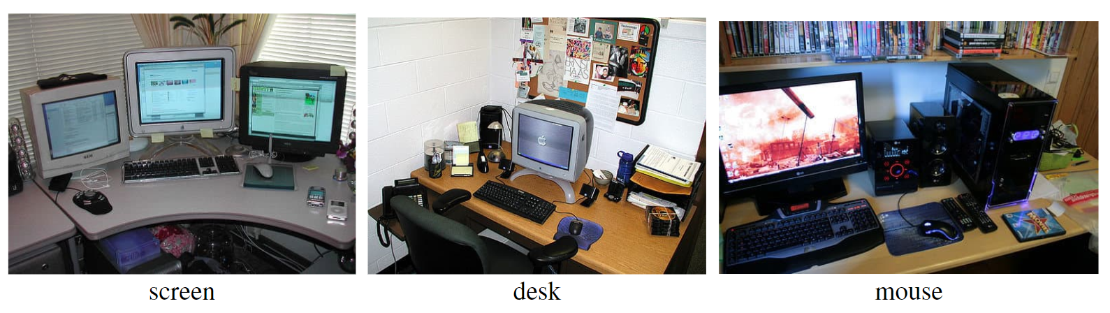
Figure 10: Example images of the classes screen, desk and mouse from ImageNet. The three classes co-occur frequently.

The velvet class has high expected-confusion with studio couch and pillow. Examples of the three classes from ImageNet are shown in Figure 11. There is a strong co-occurrence relationship because the couch and the pillows are made of materials that look like velvet.

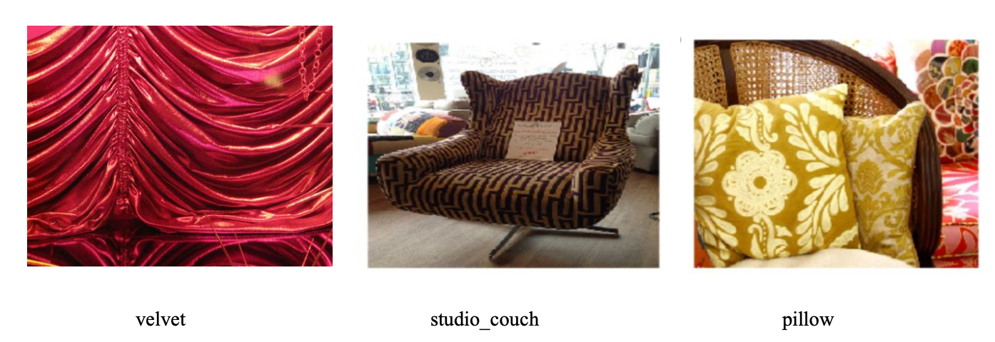
Figure 11: Example images of the classes velvet, studio couch and pillow from ImageNet. There is a strong co-occurrence relationship among the three classes because the couch and the pillows are made of materials that look like velvet

7 Imperfections in the ImageNet Dataset

Out of curiosity, we have examined images with extremely high X-perplexity (close to 1), and we found that some examples in the ImageNet might have been incorrectly or inappropriately labelled. Figure 12 shows several examples. They all have X-perplexity 1 and low C-perplexity. In other words, they are classified incorrectly by the classifiers with high confidence. As such, they are potentially mislabelled.

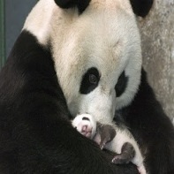
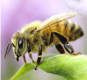
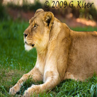
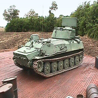
	(a)	(b)	(c)	(d)
ImageNet Label:	lesser panda	ant	hussar monkey	amphibian
X-Perplexity:	1	1	1	1
C-Perplexity:	1.00	1.14	1.00	1.15
TVL:	giant panda	bee	lion	tank

Figure 12: Potentially mislabeled images: “TVL” stands for top voted label, i.e., the class label that receives the highest number of votes from the classifiers.

Several other examples are shown in Figure 13. Their X-perplexity values are also 1, while their C-perplexity values vary. The top labels assigned by the classifiers seem to be more appropriate than the original ImageNet labels. As such, those examples might have inappropriately labelled.

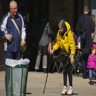
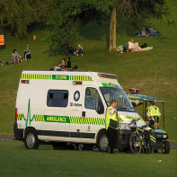
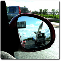
	(a)	(b)	(c)
ImageNet Label:	digital watch	golfcart	missile
X-Perplexity:	1	1	1
C-Perplexity:	14.81	1.30	1.11
TVLs:	crutch, stretcher, sax	ambulance, police van	car mirror
TELs :	crutch, stretcher, sax	police van, ambulance	car mirror, sunglasses

Figure 13: Potentially inappropriately labeled images.‘TVLs” stands for top voted labels, i.e., the class labels that receive the most number of votes from the classifiers. ‘TELs” stands for top expected labels, i.e., the class labels that have the highest expected numbers of votes from the classifiers if class assignment is done by sampling.

In Section 6, we have highlighted two reasons for high class perplexity, visually similarity between classes and class co-occurrence. An examination of highly confusing class pairs reveals a third reason: Some class labels might have been inappropriately included in the dataset. As shown in Figure 14, both corn and ear are class labels in ImageNet. It is unclear how they differ from each other. The same can be said about the confusing pair missile and projectile.

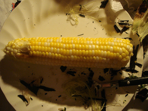
Corn	Ear	Missile	Projectile

Figure 14: Potentially problematic class labels.

8 Conclusions

In this paper, we have mainly addressed two research questions: (1) How to measure the perplexity of an example? (2) What factors contribute to high example perplexity? We propose two ways to measure example perplexity, namely C-perplexity and X-perplexity. The theory and algorithm for computing example perplexity are developed, and they are applied to ImageNet. The perplexity results on the ImageNet validation set are analyzed. Several interesting findings are made. In particular, some insights are gained regarding what makes some images harder to classify than others.

It is also found that perplexity analysis can reveal imperfections of a dataset, which can potentially help with data cleaning. This seems to be an interesting direction for further research.

Acknowledgements

Research on this paper was supported by Huawei Technologies Co., Ltd and Hong Kong Research Grants Council under grant 16204920. We also thank the deep learning computing framework MindSpore (https://www.mindspore.cn) and its team for the support on this work.

References

Appendix 1: Correlation between C-Perplexity and X-Perplexity

We can conclude the correlation relationship in one word: the X-Perplexity produced by the classifier population on ImageNet validation set is strongly correlated to C-Perplexity positively. The conclusion is suggested by Figure 15: Box Chart of C-Perplexity corresponding to different X-Perplexity classes, the relatively high Pearson Correlation coefficient 0.63644 between X-Perplexity and C-Perplexity, and the high Spearman’s Rank Correlation Coefficient 0.87425.

Figure 15: Box Chart of C-Perplexity corresponding to different X-Perplexity classes: looking the changing trend of 50% and 75% percentile line, generally with the increasing of X-Perplexity, the C-Perplexity increases also except the last X-Perplexity class.

Appendix 2: Impact of Classifier Population on Perplexity

Our classifier population includes a wide range of models with quite different prediction performance, starting from the best models trained by 100% ImageNet training images to the weakest models trained by sampled 25% training images. A remaining question here is how the perplexity is affected by the classifier population.

By the comparison of perplexity produced by different reference classifier population, we have two main findings:

a. With the increasing amount of weak classifiers in the reference classifier population, the more spread out the X-Perplexity and C-Perplexity distribution is. Figure 16 shows that most of the images with X-Perplexity closing to 0 and C-Perplexity closing to 1 under the population of strong classifiers, while the distribution under population of classifiers with mix strength is more dispersive. Similarly, from Figure 17, we can see that with more weaker classifiers adding into the population, the distribution become more and more spread out.

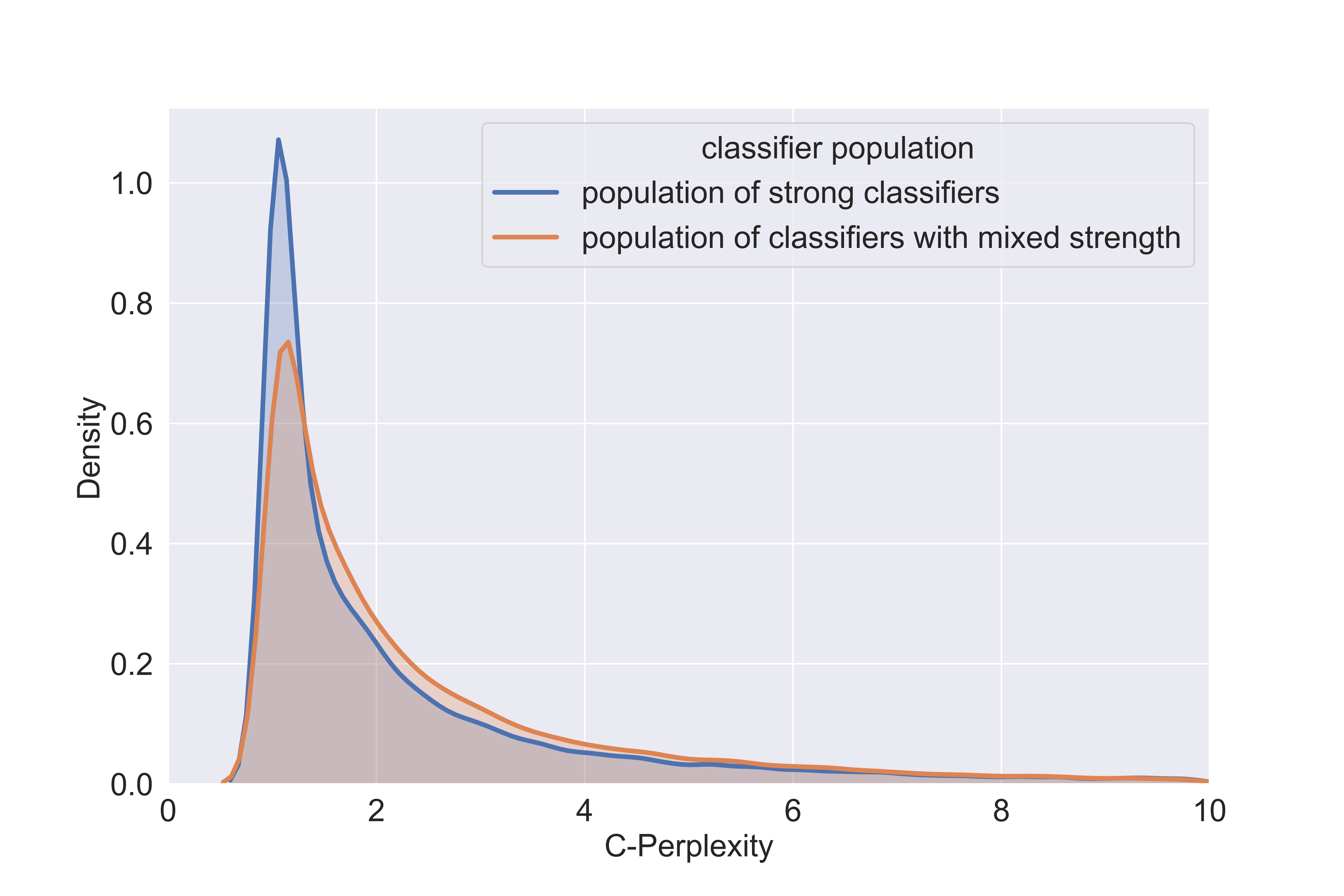
Figure 16: Comparison of X-Perplexity and C-Perplexity density plots (KDE) between population of strong classifiers (trained with 100% ImageNet training images) and population of classifiers with mixed strength (the 500 classifiers).

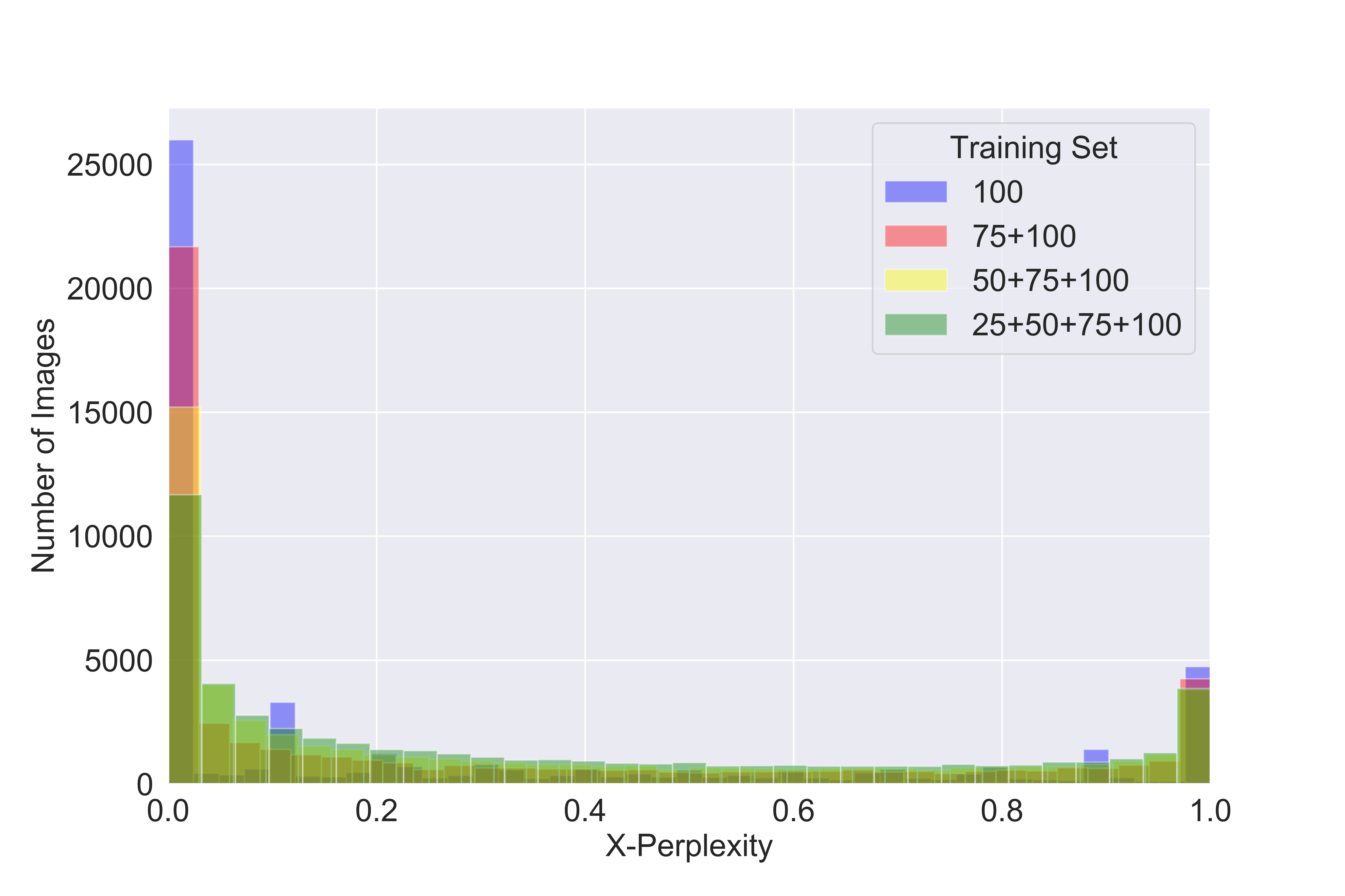
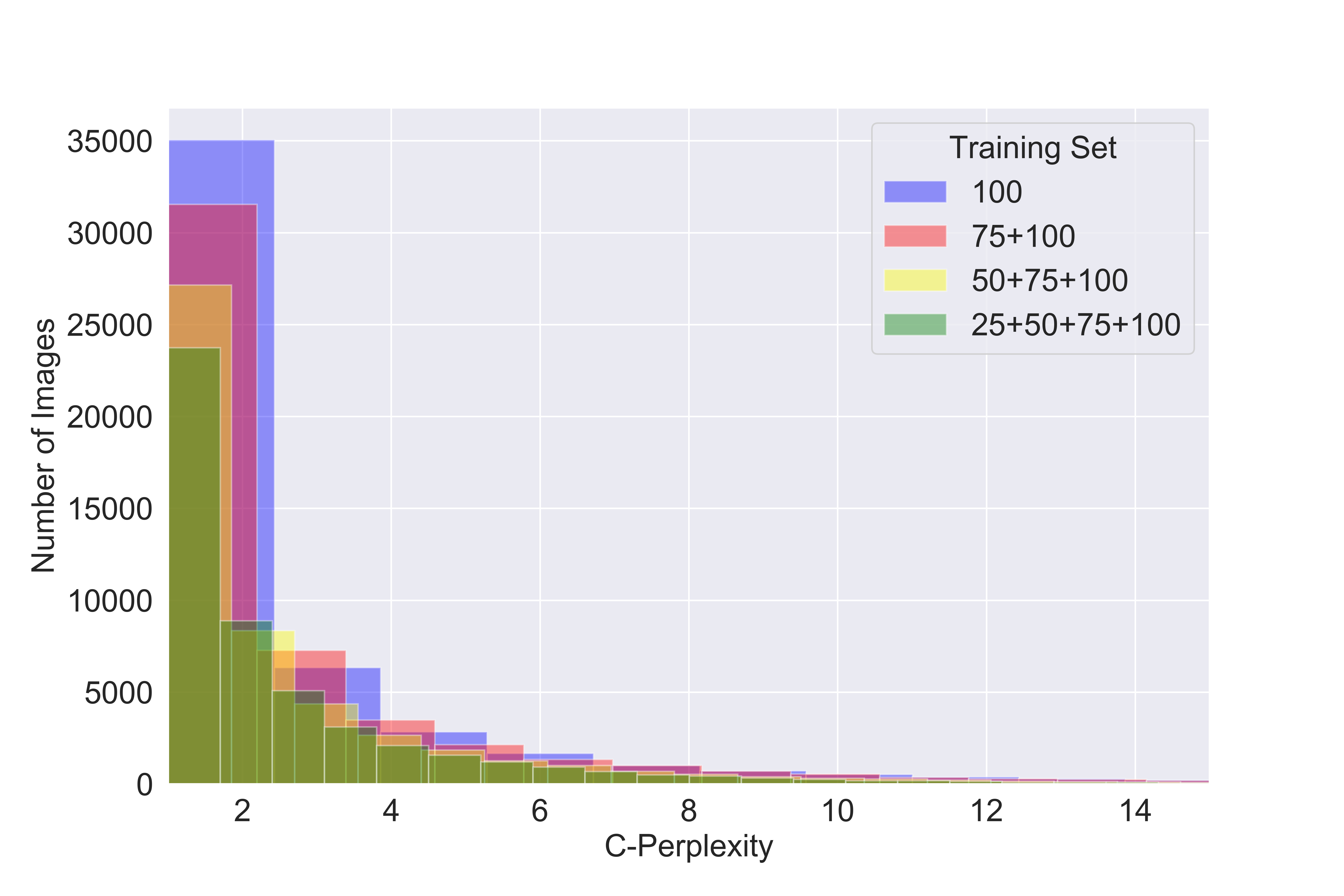
Figure 17: Comparison of X-Perplexity and C-Perplexity distribution with the adding of more weak classifiers: (1) 100-Population of best models trained by 100% ImageNet training images; (2) 75+100-Add models trained by 75% ImageNet training images into the population; (3) 50+75+100-Add models trained by 50% ImageNet training images into the population; (4) 25+50+75+100-Add models trained by 25% ImageNet training images into the population.

b. Although perplexity values vary according to the reference classifier population, the ordering they induce among the examples is stable across of a wide range of classifier populations generally. Specifically, the correlations are strong between populations with similar mixture of strong and weak classifiers. The correlations are relatively weak if the two populations have very different mixtures of strong and weak classifiers, for example one population consists of only strong classifiers and the other contains a significant fraction of weak classifiers.

The Kendall Tau correlation matrix in Figure 18 for X-Perplexity and C-Perplexity show the evidence for this point. For population of ‘Mixture(100)’ and ‘Mixture(500)’ , the mixture of strong and weak classifiers in these two population is similar and we can witness the high Kendall Tau correlation coefficient for both X-Perplexity(0.95) and C-Perplexity(0.96) between these two population. In contrast, the Kendall Tau correlation coefficient between ‘Mixture(100)’ and ‘10 strongest’ is much smaller, which is 0.61 for X-Perplexity and 0.7 for C-Perplexity.

This is another justification for the use of a population of classifiers with various strengths, since the population including mixture of weak and strong classifiers is robust enough for practical purposes while the classifiers including only strong classifiers shows lower robustness.

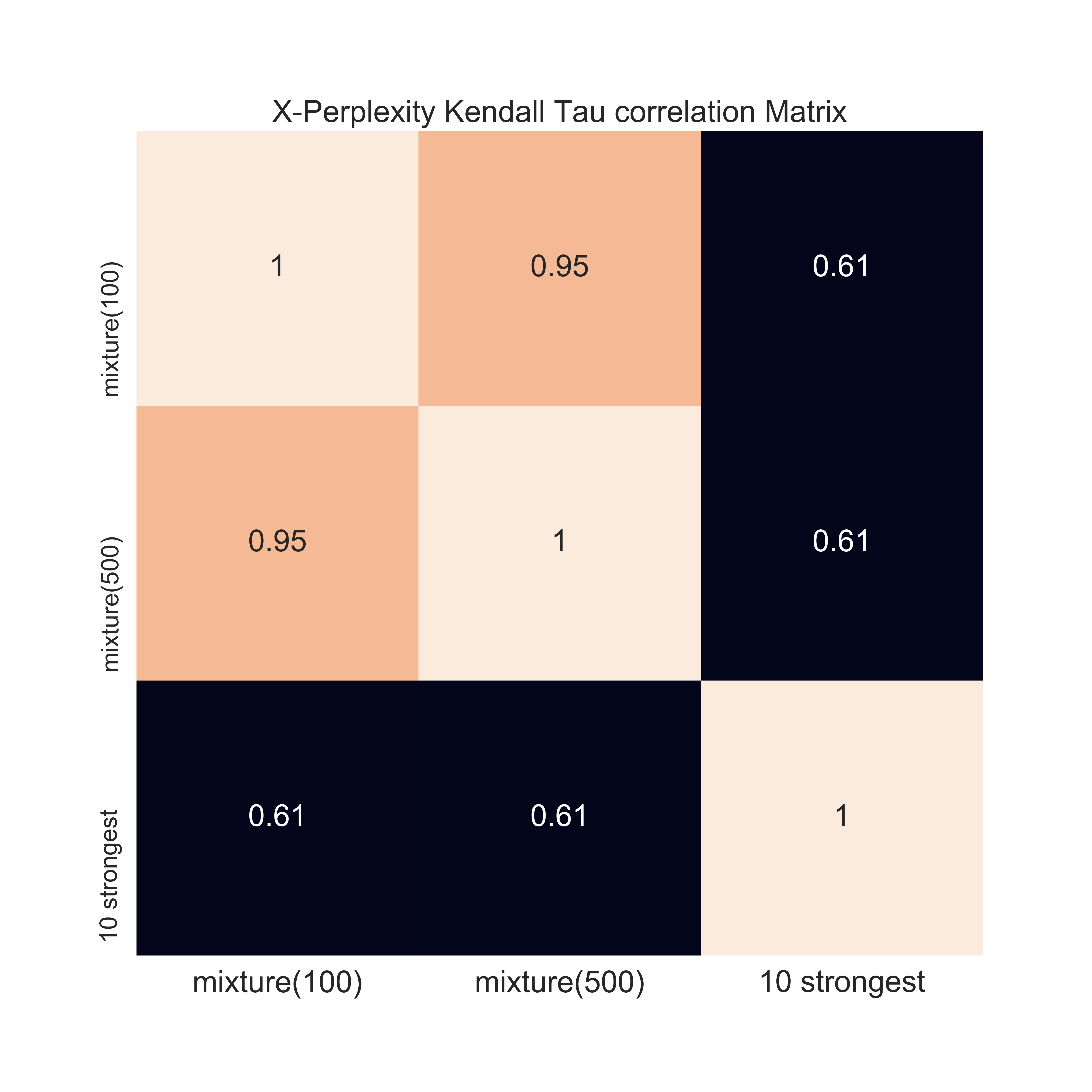
Mixture(100)- 25% ImageNet training images training model (30)+50% ImageNet training images training model (30)+75% ImageNet training images training model (30)+100% ImageNet training images training model (10);

Mixture(500)- 25% ImageNet training images training model (300)+50% ImageNet training images training model (300)+75% ImageNet training images training model (300)+100% ImageNet training images training model (100);

10 strongest: Only include 10 Best models trained by 100% ImageNet training images.

Figure 18: Kendall Tau Correlation matrix for X-Perplexity and C-Perplexity under different classifier population

References

- [1] Lucas Beyer, Olivier J Hénaff, Alexander Kolesnikov, Xiaohua Zhai, and Aäron van den Oord. Are we done with imagenet? arXiv preprint arXiv:2006.07159, 2020.
- [2] Susan E Embretson and Steven P Reise. Item response theory. Psychology Press, 2013.
- [3] Xiaoxiao Li, Ziwei Liu, Ping Luo, Chen Change Loy, and Xiaoou Tang. Not all pixels are equal: Difficulty-aware semantic segmentation via deep layer cascade. In Proceedings of the IEEE conference on computer vision and pattern recognition, pages 3193–3202, 2017.
- [4] Dong Nie, Li Wang, Lei Xiang, Sihang Zhou, Ehsan Adeli, and Dinggang Shen. Difficulty-aware attention network with confidence learning for medical image segmentation. In Proceedings of the AAAI Conference on Artificial Intelligence, volume 33, pages 1085–1092, 2019.
- [5] Florian Scheidegger, Roxana Istrate, Giovanni Mariani, Luca Benini, Costas Bekas, and Cristiano Malossi. Efficient image dataset classification difficulty estimation for predicting deep-learning accuracy. The Visual Computer, pages 1–18, 2020.
- [6] Dimitris Tsipras, Shibani Santurkar, Logan Engstrom, Andrew Ilyas, and Aleksander Madry. From imagenet to image classification: Contextualizing progress on benchmarks. arXiv preprint arXiv:2005.11295, 2020.
- [7] Radu Tudor Ionescu, Bogdan Alexe, Marius Leordeanu, Marius Popescu, Dim P Papadopoulos, and Vittorio Ferrari. How hard can it be? estimating the difficulty of visual search in an image. In Proceedings of the IEEE Conference on Computer Vision and Pattern Recognition, pages 2157–2166, 2016.
- [8] Shuang Yu, Hong-Yu Zhou, Kai Ma, Cheng Bian, Chunyan Chu, Hanruo Liu, and Yefeng Zheng. Difficulty-aware glaucoma classification with multi-rater consensus modeling. arXiv preprint arXiv:2007.14848, 2020.