Significance of chiral three-nucleon force contact terms for understanding of elastic nucleon-deuteron scattering

Abstract

We investigate the importance of the three-nucleon (3N) force contact terms in elastic nucleon-deuteron (Nd) scattering by applying the N⁴LO⁺ chiral semi-local momentum space (SMS) regularized nucleon-nucleon (NN) chiral potential supplemented by N²LO and all subleading N⁴LO three-nucleon force (3NF) contact terms. Strength parameters of the contact terms were obtained by least squares fitting of theoretical predictions to cross section and analyzing powers data at three energies of the impinging nucleon. Although the N³LO contributions to the 3N force were completely neglected, the results calculated with the contact terms multiplied by the fitted strength parameters yield an improved description of the elastic Nd scattering observables in a wide range of incoming nucleon energies below the pion production threshold.

I Introduction

Since the advent of numerically exact 3N Faddeev calculations [1, 2, 3] numerous clear-cut discrepancies between data and theoretical predictions have been found for observables in the elastic Nd scattering and deuteron breakup reactions. Surprisingly, the magnitudes of these discrepancies are to a large degree independent of the dynamical ingredients used in the calculations. They are comparable for calculations which employ high-precision (semi)phenomenological two-nucleon (2N) potentials supplemented by standard models of 3N forces (3NF) and for predictions obtained with the chiral NN and 3N N²LO interactions. The low-energy analyzing power puzzle – a clear underestimation of the maximum of the vector analyzing power in neutron-deuteron (nd) and proton-deuteron (pd) elastic scattering at low incoming nucleon laboratory energies (below $\approx 25$ MeV) – is one of the best known cases [4]. The underprediction of the elastic scattering angular distribution, starting at $\approx 60$ MeV, in the region of the c.m. cross section minimum, which extends to the backward c.m. angles and grows with the incoming nucleon energy [5] or a large gap at higher energies between the measured total cross section for the nd interaction and theoretical predictions [6, 7] are further examples of such discrepancies. Also the breakup reaction provides data which remain unexplained and the most prominent case is the cross section of the low-energy space-star geometry in the complete nd and pd breakup [8].

In the standard approach to a 3N continuum one selects a high-precision NN potential and augments it by some model of a 3N force, whose parameters provide a satisfactory description of the triton binding. The 3N continuum Faddeev equation is solved with such dynamical input and predictions for observables are made. For (semi)phenomenological potentials such an attitude is from the very beginning disputable due to the inconsistency between applied 2N and 3N interactions. The situation dramatically changed with the availability of chiral two- and many-body forces derived consistently in the framework of chiral perturbation theory ($\chi$PT) [9, 10, 11, 12, 13, 14, 15]. The high precision of the description of 2N data achieved by recent N⁴LO⁺ SMS NN potential of the Bochum group [16] together with the derivation of 3N forces up to N⁴LO order of the chiral expansion [17, 18, 19, 20, 21] provided a solid basis for a successful description of 3N continuum. However, in spite of great expectations the results of investigations performed up to now with the chiral 3N forces restricted to the third order (N²LO) of the chiral expansion, show that this new dynamics leads practically to the same 3N data description as the (semi)phenomenological 2N and 3N interactions [22, 23]. It means that the chiral 3NF at N²LO, which contains a 2$\pi$-exchange parameter free component supplemented by two contact terms [17], is more or less equivalent to the commonly used Urbana IX [24] or TM99 [25] 3NF’s.

The situation changed when the Pisa group published results of calculations for elastic pd scattering below the deuteron breakup threshold obtained with 3NF containing subleading N⁴LO chiral contact terms [26]. They showed that it is possible to correctly describe the elastic pd scattering data together with the ³H binding energy by augmenting the Urbana IX 3NF with the N⁴LO 3NF contact terms. It indicated that very probably the missing part of the 3N dynamics in up to now performed 3N continuum calculations, namely omitted N⁴LO contact terms, could be the reason for difficulties in explaining the discrepancies mentioned above. That offers a real prospect of even deeper understanding of 3N continuum data up to the pion production threshold, when chiral 3N continuum calculations with best chiral NN interaction, supplemented by a chiral 3NF at least up to an N³LO order of chiral expansion and including all subleading N⁴LO contact terms, becomes available.

The first nonvanishing contributions to the 3N force appear at N²LO [10, 17] and comprise, in addition to the parameter-free $2\pi$-exchange term, two contact contributions with strength parameters $c_{D}$ and $c_{E}$ [17, 27]. Since the chiral 3NF acquires at N³LO only parameter-free contributions, with all N⁴LO contact terms the 3N Hamiltonian depends additionally on 13 strength parameters $c_{E_{i}}$ of these short-range 3NF components [28, 29]. Since two pairs of N⁴LO contact terms are identical, the number of free parameters in the 3N Hamiltonian reduces eventually to 13. They must be fixed by a fit to the 3N data. This task is comparable if not easier than in the case of the 2N system, where the Hamiltonian required determination of 15 free parameters [16]. In the 2N system fitting parameters to 2N continuum data automatically provided the correct deuteron binding energy. One can hope that also for the 3N system strength parameters of the 3NF contact terms obtained by fitting theoretical predictions for different observables to 3N continuum data will lead to a 3N Hamiltonian able to reproduce the binding energies of ³H and ³He.

Using a chiral 3NF in 3N continuum calculations requires numerous time consuming computations with varying strengths of the contact terms in order to establish their values. Fine-tuning of the 3N Hamiltonian parameters requires an extensive analysis of available 3N elastic Nd scattering and breakup data. That ambitious goal calls for a significant reduction of computer time necessary to solve the 3N Faddeev equations and to calculate the observables. Thus finding an efficient emulator for exact solutions of the 3N Faddeev equations seems to be essential and of high priority.

In Ref. [30] we proposed such an emulator which enabled us to reduce significantly the required time of calculations. We tested its efficiency as well as ability to accurately reproduce exact solutions of 3N Faddeev equations. In Ref. [31] we introduced a new computational scheme, based on the perturbative approach of [30], which even by far more reduced the computer time necessary to obtain the observables in the elastic nucleon-deuteron scattering and deuteron breakup reactions at any energy, and which is well-suited for calculations with varying strengths of the contact terms in a chiral 3NF.

This development of the efficient emulator for 3N continuum calculations enables us to perform an investigation of 3N continuum with the inclusion of all 3NF contact terms up to the fifth order (N⁴LO) of the chiral expansion. Our aim is to check whether by using the best available chiral NN potential augmented by the recently developed consistent N²LO 3NF components [22, 23] and including all contact terms up to N⁴LO order of chiral expansion it is possible to fix parameters of the 3N Hamiltonian by fitting the theoretical predictions to the 3N continuum data basis. Furthermore, we will verify if such a Hamiltonian will simultaneously reproduce the ³H and ³He binding energies as well as the nd doublet scattering length ${}^{2}a_{nd}$. In addition we would like to examine what impact such an Hamiltonian will have on the description of the 3N continuum, e.g. whether its use will eliminate or reduce the discrepancies mentioned earlier.

The paper is organized as follows. In Sec.II for the convenience of the reader we describe the most essential points of our approach to 3N continuum calculations, especially the new emulator and very fast and efficient scheme for the computation of elastic scattering observables. The results on importance of contributions from different N²LO and N⁴LO contact terms to numerous nd elastic scattering observables as well as on a sensitivity pattern of these contributions are shown in Sec.III. In Sec.IV we determine the strengths of contact terms by fitting theoretical predictions to elastic scattering data and verify whether the established Hamiltonian leads to an improved description of Nd elastic scattering data. We summarize and conclude in Sec.V.

II Theory

For the reader’s convenience we briefly outline the 3N Faddeev formalism and the perturbative treatment of Ref. [30]. For details of the Faddeev formalism and numerical performance we refer the reader to  [1, 33, 34, 32].

The 3N Hamiltonian comprises pairwise interactions $v_{NN}=v_{12}+v_{23}+v_{31}$ and a 3N force $V_{123}=V^{(1)}+V^{(2)}+V^{(3)}$, where the latter is decomposed into three Faddeev components $V^{(i)}$, symmetric in the particle labels $j,k\neq i\in\{1,2,3\}$. Since nucleons are treated as identical particles, it is possible to single out the $(2,3)$ subsystem and use only $V^{(1)}$ in the Faddeev-type integral equation for the breakup operator $T$, which describes Nd scattering [1, 33, 34]

$$T|\phi\rangle = tP|\phi\rangle+(1+tG_{0})V^{(1)}(1+P)|\phi\rangle+tPG_{0}T|\phi\rangle$$ (1)

$$+ (1+tG_{0})V^{(1)}(1+P)G_{0}T|\phi\rangle\,.$$ (2)

The initial state $|\phi\rangle=|\vec{q}_{0}\rangle|\phi_{d}\rangle$ describes the free motion of the neutron and the deuteron with the relative momentum $\vec{q}_{0}$ and contains the internal deuteron wave function $|\phi_{d}\rangle$. The amplitude for elastic scattering leading to the final nd state $|\phi^{\prime}\rangle$ is then given by [1, 34]

$$\langle\phi^{\prime}|U|\phi\rangle = \langle\phi^{\prime}|PG_{0}^{-1}|\phi\rangle+\langle\phi^{\prime}|V^{(1)}(1+P)|\phi\rangle$$ (3)

$$+ \langle\phi^{\prime}|V^{(1)}(1+P)G_{0}T|\phi\rangle+\langle\phi^{\prime}|PT|\phi\rangle~{},$$ (4)

while the amplitude for the breakup reaction reads

$$\langle\vec{p}\vec{q}|U_{0}|\phi\rangle = \langle\vec{p}\vec{q}|(1+P)T|\phi\rangle,$$ (5)

where the free breakup channel state $|\vec{p}\vec{q}\rangle$ is defined in terms of the Jacobi (relative) momenta $\vec{p}$ and $\vec{q}$.

We solve Eq. (2) in the momentum-space partial-wave basis $|pq\alpha\rangle$, determined by the magnitudes of the Jacobi momenta $p$ and $q$ and a set of discrete quantum numbers $\alpha$ comprising the 2N subsystem spin, orbital and total angular momenta $s,l$ and $j$, as well as the spectator nucleon orbital and total angular momenta with respect to the center of mass (c.m.) of the 2N subsystem, $\lambda$ and $I$:

$$|pq\alpha\rangle\equiv|pq(ls)j(\lambda\frac{1}{2})I(jI)J(t\frac{1}{2})T\rangle~{}.$$ (6)

The total 2N and spectator angular momenta $j$ and $I$ as well as isospins $t$ and $\frac{1}{2}$, are finally coupled to the total angular momentum $J$ and isospin $T$ of the 3N system, respectively. In practice a converged solution of Eq. (2) using partial wave decomposition in momentum space at a given energy $E$ requires taking all 3N partial wave states up to the 2N angular momentum $j_{max}=5$ and the 3N angular momentum $J_{max}=\frac{25}{2}$, with the 3N force acting up to the 3N total angular momentum $J=7/2$. The number of resulting partial waves for given $J$ (equal to the number of coupled integral equations in two continuous variables $p$ and $q$) amounts to $142$. The required computer time to get one solution on a personal computer is about few hours. In the case when such calculations have to be performed for a big number of varying 3NF parameters, time restrictions become prohibitive.

The perturbative approach proposed in Ref. [30] and [31] leads to a significant reduction of the required computational time. It relies on the fact that it is possible to apply a perturbative approach in order to include the contact terms in 3N continuum calculations. Let us consider a chiral 3NF $V^{(1)}$ at a given order of chiral expansion with variable strengths of its contact terms. The contact terms are restricted to small 3N total angular momenta and to only few partial wave states for a given total 3N angular momentum $J$ and parity $\pi$ [17, 27]. We split the $V^{(1)}$ into a parameter-free term $V(\theta_{0})$ and a sum of $N$ contact terms $c_{i}\Delta V_{i}$ with strengths $c_{i}$:

$$V^{(1)} = V(\theta_{0})+\Delta V(\theta)=V(\theta_{0})+\sum_{i=1}^{N}c_{i}\Delta V_{i}~{},$$ (7)

with $\theta_{0}=(c_{i}=0,i=1,\dots,N)$ and $\theta=(c_{i},i=1,\dots,N)$ being the sets of contact terms strength values, for which we would like to find solution of Eq. (2).

We divide the 3N partial wave states into two sets: $\beta$ and the remaining one, $\alpha$. The $\beta$ set is defined by nonvanishing matrix elements of $\Delta V(\theta)$. Introducing $T(\theta_{0})$ and $\Delta T(\theta)$ such that $T\equiv T(\theta)=T(\theta_{0})+\Delta T(\theta)$, and using the fact that $\Delta V(\theta)$ has nonvanishing elements only for channels $|\beta\rangle$, one gets from Eq. (2) two separate sets of equations for $\langle\alpha|T(\theta_{0})|\phi\rangle$ and $\langle\alpha|\Delta T(\theta)|\phi\rangle$ (Eqs.(9) and (10) in [30] or Eqs.(6) and (7) in [31]). The first equations in sets (6) and (7) of Ref. [31] are the Faddeev equations (2) for $T(\theta_{0})$. The second equation in the set (7) for $\langle\beta|\Delta T(\theta)|\phi\rangle$ can be solved within the set of channels $|\beta\rangle$ only. Since $\Delta V(\theta)$ is small, it is possible to neglect the term $\langle\beta|(1+tG_{0})\Delta V(\theta)(1+P)G_{0}\Delta T(\theta)|\phi\rangle$ in the kernel and arrive at the following integral equation for $\langle\beta|\Delta T(\theta)|\phi\rangle$:

$$\langle\beta|\Delta T(\theta)|\phi\rangle = \langle\beta|(1+tG_{0})\Delta V(\theta)(1+P)|\phi\rangle$$ (8)

$$+ \langle\beta|(1+tG_{0})\Delta V(\theta)(1+P)G_{0}T(\theta_{0})|\phi\rangle$$ (9)

$$+ \langle\beta|(1+tG_{0})V(\theta_{0})(1+P)G_{0}\Delta T(\theta)|\phi\rangle$$ (10)

$$+ \langle\beta|tPG_{0}\Delta T(\theta)|\phi\rangle~{}.$$ (11)

That equation permits one to transfer the linear dependence on the strengths $c_{i}$ from the $\Delta V(\theta)$ on the $\Delta T(\theta)$. Namely, let $\langle\beta|\Delta T_{i}|\phi\rangle$ be a solution of Eq.(11) for a set $\theta_{i}=(c_{i}=1,c_{k\neq i}=0)$:

$$\langle\beta|\Delta T_{i}|\phi\rangle \equiv \langle\beta|(1+tG_{0})\Delta V_{i}(1+P)|\phi\rangle$$ (12)

$$+ \langle\beta|(1+tG_{0})\Delta V_{i}(1+P)G_{0}T(\theta_{0})|\phi\rangle$$ (13)

$$+ \langle\beta|(1+tG_{0})V(\theta_{0})(1+P)G_{0}\Delta T_{i}|\phi\rangle$$ (14)

$$+ \langle\beta|tPG_{0}\Delta T_{i}|\phi\rangle~{}.$$ (15)

then the solution of Eq. (11) is given by:

$$\langle\beta|\Delta T(\theta)|\phi\rangle = \sum_{i=1}^{N}c_{i}\langle\beta|\Delta T_{i}|\phi\rangle~{}.$$ (16)

In this way at a given energy the computation of observables in the elastic Nd scattering and deuteron breakup reaction for any combination of strengths $c_{i}$ of contact terms is reduced to solving once $N+1$ Faddeev equations: one equation for $T(\theta_{0})$ and N equations for $\Delta T_{i}$. In the first step, solution for $\langle\alpha(\beta)|T(\theta_{0})|\phi\rangle$ is found. Then Eq. (15) is solved for $\langle\beta|\Delta T_{i}|\phi\rangle$, from which the $\langle\alpha|\Delta T_{i}|\phi\rangle$ is calculated by:

$$\langle\alpha|\Delta T_{i}|\phi\rangle = \langle\alpha|tPG_{0}\sum_{\beta}\int_{p^{\prime}q^{\prime}}|p^{\prime}q^{\prime}\beta\rangle\langle p^{\prime}q^{\prime}\beta|\Delta T_{i}|\phi\rangle$$ (17)

$$+ \langle\alpha|(1+tG_{0})V(\theta_{0})(1+P)G_{0}$$ (19)

$$\sum_{\beta}\int_{p^{\prime}q^{\prime}}|p^{\prime}q^{\prime}\beta\rangle\langle p^{\prime}q^{\prime}\beta|\Delta T_{i}|\phi\rangle~{}.$$

The computations described above need to be done only once and then for any combination of the strengths $c_{i}$ $\langle\alpha(\beta)|T(\theta=(c_{i},i=1,\dots,N))|\phi\rangle$ is obtained by trivial summation:

$$\langle\alpha|T(\theta)|\phi\rangle = \langle\alpha|T(\theta_{0})|\phi\rangle+\sum_{i}c_{i}\langle\alpha|\Delta T_{i}|\phi\rangle$$ (20)

$$\langle\beta|T(\theta)|\phi\rangle = \langle\beta|T(\theta_{0})|\phi\rangle+\sum_{i}c_{i}\langle\beta|\Delta T_{i}|\phi\rangle~{}.$$ (21)

For a calculation of elastic scattering observables the required sum of the second and the third term in Eq. (4) is obtained by:

$$\langle\alpha|V^{(1)}(\theta)(1+P)|\phi\rangle+\langle\alpha|V^{(1)}(\theta)(1+P)G_{0}T(\theta)|\phi\rangle=$$ (22)

$$\langle\alpha|V(\theta_{0})(1+P)|\phi\rangle+\langle\alpha|V(\theta_{0})(1+P)G_{0}T(\theta_{0})|\phi\rangle$$ (23)

$$+\sum_{i}c_{i}[\langle\alpha|\Delta V_{i}(1+P)|\phi\rangle+\langle\alpha|\Delta V_{i}(1+P)G_{0}T(\theta_{0})|\phi\rangle$$ (24)

$$+\langle\alpha|V(\theta_{0})(1+P)G_{0}\Delta T_{i}|\phi\rangle]$$ (25)

$$+\sum_{i,k}c_{i}c_{k}\langle\alpha|\Delta V_{i}(1+P)G_{0}\Delta T_{k}|\phi\rangle~{}.$$ (26)

This computational scheme constitutes the improved emulator of Ref. [31]. The efficiency of the fitting procedure based on this emulator can be further increased because the elastic scattering $\langle\phi^{\prime}|U|\phi\rangle$ and breakup $\langle\vec{p}\vec{q}|U_{0}|\phi\rangle$ transition amplitudes are linear in the matrix elements $\langle pq\alpha|T|\phi\rangle$. Therefore also the final transition matrix elements are linked to the strengths $c_{i}$ in the same way as shown in Eqs.(21) and (26). It allows us at a given energy to perform only once all required interpolations, integrations over Jacobi momenta, as well as summations over the partial waves, total angular momenta and parities, to gain the contributions to the transition amplitudes, which are independent from the actual values of strengths $c_{i}$. Finally, the transition amplitudes for any particular set of strengths $c_{i}$ are obtained from the same simple relations as in Eqs.(21) and (26). It reduces radically the required time to compute observables and permits to get observables for hundreds of strengths combinations in the blink of an eye. An additional beneficial feature of that emulator, which makes it especially well-suited for optimization purposes, is the simple dependence of the transition amplitudes on the strengths $c_{i}$, enabling fast and easy access to the gradient with respect to strength parameters for any observable.

III Importance of contact terms in elastic nd scattering

Equipped with the new emulator we investigate the significance of the 3NF contact terms for understanding the Nd elastic scattering. To this end we take the state-of-the-art chiral SMS N⁴LO⁺ NN potential of the Bochum group [16] with the regularization parameter $\Lambda=450$ MeV, combined with the N²LO chiral 3NF [17] and supplemented by all subleading N⁴LO 3NF contact terms [28, 29]. Such a Hamiltonian comprises altogether 15 short range contributions to 3NF, two from N²LO [10, 17] with the strengths $D$ and $E$, and thirteen from N⁴LO [29] with the strengths $E_{i},i=1,\dots,13$. To all these contact terms we applied the same nonlocal Gaussian regulator defined in Eq. (13) of Ref.[27] with the cutoff parameter $\Lambda=450$ MeV. The strengths $D$, $E$, and $E_{i}$ can be expressed by dimensionless coefficients $c_{D}$, $c_{E}$, and $c_{E_{i}}$ according to [27]:

$$D=\frac{c_{D}}{F^{2}_{\pi}\Lambda_{\chi}},~{}~{}E=\frac{c_{E}}{F^{4}_{\pi}\Lambda_{\chi}},~{}~{}E_{i}=\frac{c_{E_{i}}}{F^{4}_{\pi}\Lambda^{3}_{\chi}}~{},$$ (27)

where $F_{\pi}=92.4$ MeV is the pion decay constant and $\Lambda_{\chi}=700$ MeV.

In order to explore the role of contact terms in 3N continuum, partial wave decomposition (PWD) of these 3NF components must be performed in the momentum space. It has been done in a standard way [32, 35]. The corresponding expressions for $D$ and $E$ terms can be found in Ref.[17] and for $E_{1}$ and $E_{7}$ terms in Ref.[27]. For the remaining N⁴LO contact terms the choice of the Faddeev component and its PWD are given in the Appendix. It turned out that PWD for the $E_{9}$ and $E_{11}$ terms yields the same result. The same was found for the $E_{10}$ and $E_{12}$ terms. Thus only 11 out of 13 N⁴LO contact terms are independent.

In view of the large number of contributing short-range terms one can ask the question, whether it is at all possible to find the unambiguous magnitudes of all these strengths using available Nd elastic scattering data. Only if the answer is affirmative, valuable predictions based on the resulting 3N Hamiltonian can be obtained.

Before we answer this pivotal question, let us consider the patterns, according to which short range 3NF terms contribute to different Nd elastic scattering observables. In particular it should be examined if some terms are more important than others for a specific class of observables, and how a pattern of sensitivity to different 3NF contact terms is changing with energy.

To that end we performed the 3N continuum Faddeev calculations at five laboratory energies of the incoming neutron $E=10$, $70$, $135$, $190$, and $250$ MeV using the dynamical input defined above and our emulator.

The selected energies cover the range of interesting discrepancies between theory and data mentioned in the introduction. To find out the pattern of sensitivity to a particular short range component we calculated at these energies all elastic nd scattering observables adding consecutively to the parameter free 3NF part $V(\theta_{0})$ only one component with a strength $c_{E_{i}}$ varied between $c_{E_{i}}=-2.0$ up to $c_{E_{i}}=+2.0$. The set of elastic scattering observables (55 in total) comprised the differential cross section, nucleon vector and deuteron vector and tensor analyzing powers, spin correlation coefficients, nucleon to nucleon, nucleon to deuteron, deuteron to nucleon and deuteron to deuteron spin transfer coefficients. For each observable we studied angular variations of predictions themselves as well as a quantity $\Delta$ which shows the sign and magnitude of the percent deviation from the prediction with the parameter free 3NF term ($V(\theta_{0})$) induced by that specific 3NF component, averaged over all c.m. angles $\theta_{k}$. Specifically, for a particular observable Obs, and for only one short range term with the strength $c_{j}$ active, ($c_{j}$ is one of the strength $c_{D}$, $c_{E}$, or $c_{E_{i}},i=1,\dots,10,13$), the quantity $\Delta$ is defined by:

$$\Delta\equiv\Delta(c_{j})=\frac{1}{N_{\theta}}\sum_{\theta_{k}}\frac{Obs(c_{j},\theta_{k})-Obs(\theta_{0},\theta_{k})}{Obs(\theta_{0},\theta_{k})}\times 100\%~{},$$ (28)

with $N_{\theta}=73$ and step of $\theta_{k}$ equal $2.5^{\circ}$.

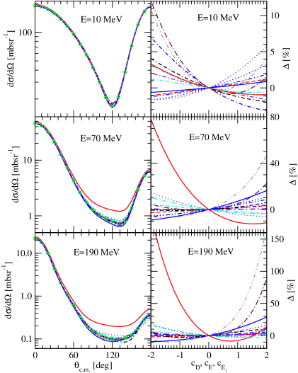
Figure 1: (color online) (left column) The elastic nd scattering differential cross section $\frac{d\sigma}{d\Omega}$ at the incoming neutron laboratory energies $E=10,70,$ and $190$ MeV. The lines depicted by (green) circles show the results obtained with the SMS N⁴LO⁺ NN potential with the regularization parameter $\Lambda=450$ MeV, supplemented by the parameter-free 2$\pi$-exchange N²LO 3NF. Other lines are the results when the above dynamics is augmented with a single contact term of strength $c_{i}=-1.0$: $D$ - (red) short-dashed, $E$ - (blue) short-dashed-dotted, $E_{1}$ - (blue) dotted, $E_{2}$ - (violet) short-dashed-dotted, $E_{3}$ - (cyan) short-dashed-dotted, $E_{4}$ - (maroon) long-dashed-dotted, $E_{5}$ - (brown) short-dashed-double-dotted, $E_{6}$ - (black) double-dashed-dotted, $E_{7}$ - (blue) solid, $E_{8}$ - (red) solid, $E_{9}$ - (turquoise) double-dashed-dotted, $E_{10}$ - (indigo) dotted, and $E_{13}$ - (blue) dashed-double-dotted. In the right column a percentage deviations $\Delta$ (see text) of the single contact term predictions with respect to the parameter-free part of the N²LO 3NF $V(\theta_{0})$ are shown as a function of the strength $c_{i}$. The lines in the right column correspond to those in the left column.

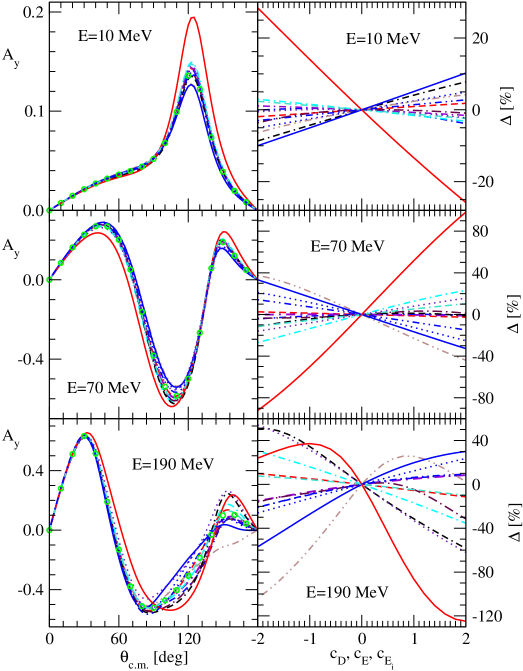
Figure 2: (color online) The same as in Fig.1 but for the nucleon analyzing power $A_{y}$.

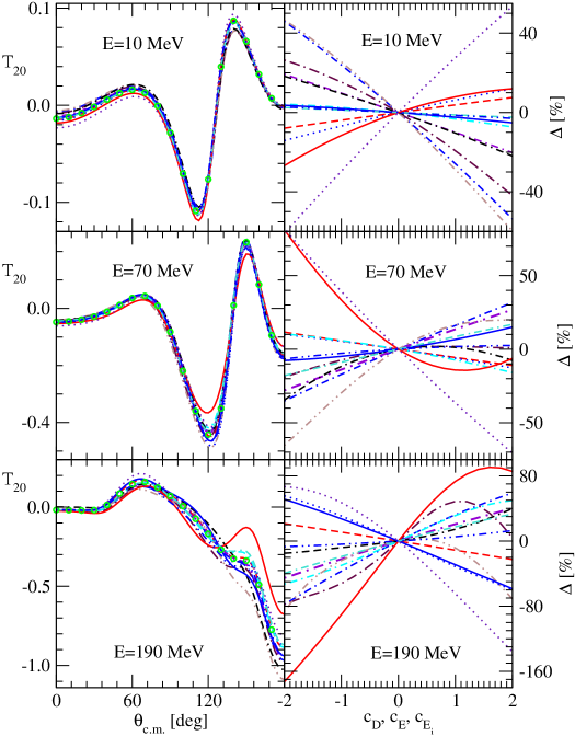
Figure 3: (color online) The same as in Fig.1 but for the deuteron tensor analyzing power $T_{20}$.

In Figs.1-3 we show the results of this investigation for three observables: the differential cross section $\frac{d\sigma}{d\Omega}$, the nucleon analyzing power $A_{y}$, and the deuteron tensor analyzing power $T_{20}$, at three energies $E=10$, $70$, and $190$ MeV. In the left column predictions for these observables, obtained with parameter free part of the N²LO 3NF $V(\theta_{0})$, as well as including in addition consecutively each of the 13 short range terms, are shown as a function of the c.m. scattering angle $\theta$. In the right column the quantity $\Delta$ is displayed for that particular observable and for each of the 13 short range terms, as a function of their strengths.

The pattern of sensitivities exemplified in Figs.1-3 reflects the features common for all studied observables. At low energy $E=10$ MeV the changes induced by different short-range components are of the order of about few percent, with the exception of few terms, which affect significantly a particular observable (see for example Fig. 2 displaying the dominating impact of the $E_{8}$ term on $A_{y}$). With increasing energy the pattern changes both with respect to the magnitudes of the induced changes and with respect to the number of appreciably contributing terms. For the cross section (see Fig.1) the magnitude of $\Delta$ reaches approximately 100 % at $190$ MeV with the dominating contributions coming from the $E_{5}$ and $E_{8}$ terms. Similarly, for $A_{y}$ (Fig.2) and $T_{20}$ (Fig.3) $E_{8}$ prevails at higher energies and its effects have opposite signs at $70$ MeV and $190$ MeV. Such alternating patterns of sensitivities with respect to the observable, energy, and contributing short-range contact term, foreshadow a successful determination of all the contact terms strengths by fitting theoretical predictions to Nd elastic scattering data.

It should be emphasised that practically for most of the studied observables and energies, the contributions from the N²LO $D$ and $E$ contact terms, expressed in terms of $\Delta$, do not belong to the most significant ones. In view of that, to determine how important the N⁴LO contact terms are for the 3N bound system, we calculated their expectation values in the triton arising from the N⁴LO⁺ SMS NN force ($\Lambda=450$ MeV) alone, taking their strengths $c_{i}=1.0$. (see Table 1). It is clear that nearly all short-range terms, with the exception of the $E_{7}$ and $E_{8}$ terms providing negligible contributions, make comparable and significant contributions to the triton potential energy. Therefore the subleading contact terms seem to play a significant role not only in 3N continuum but also in the bound states.

IV Fixing strengths of contact terms

Let us come back to the basic question, how precisely and reliably all the strengths of the 3NF short-range components can be determined. The results of the previous section are promising, since they reveal a pattern of high sensitivity (changing with the observable and energy) to practically all the short-range components of the considered chiral 3NF but this is only a necessary condition. The decisive is the quality and number of available Nd elastic scattering data points. As a consequence of strenuous efforts of experimentalists the amount and precision of the available pd data has recently radically improved. Still, the presently accessible pd data base is not so numerous as the proton-proton (pp) one. Below the pion production threshold pd data have been taken at a number of energies on the elastic scattering cross section, proton analyzing power, all deuteron vector and tensor analyzing powers, and in few cases some polarization transfer and spin correlation coefficients. For the nd data basis the situation is worse and only at few energies nd elastic scattering cross sections and neutron analyzing powers are available, with larger errors than in the case of the pd data. In addition, for the nd system also high precision data for the total nd cross section have been collected.

In the first step we investigate if the alternating pattern of large sensitivities found in the previous section and access to high quality Nd data would be sufficient for a successful determination of all the strengths. To be specific, we assume that we have high quality data for the cross section, the nucleon analyzing power and the deuteron vector and tensor analyzing powers. We generated such pseudo-data at five energies $E=10,70,135,190,$ and $250$ MeV, using our dynamical input and taking all 13 strengths $c_{i}=1.0$. The data covered the range of the c.m. angles $\theta_{c.m.}\in(40^{\circ}-170^{\circ})$ with a step of $5^{\circ}$ and had the preconditioned relative error of $5~{}\%$. To these data we applied the least-squares method by introducing the $\chi^{2}(c_{i})$ merit function:

$$\chi^{2}(c_{i}) = \sum_{Obs,\theta_{k},E}[\frac{Obs^{th}(c_{j},\theta_{k},E)-Obs^{ex}(\theta_{k},E)}{\Delta Obs^{ex}(\theta_{k},E)}]^{2}~{},$$ (29)

and looked for minimum of $\chi^{2}(c_{i})$ with respect to the strengths $c_{i}$. To find the minimum we applied the Levenberg-Marquard method [36, 37], which, in addition to $\chi^{2}$ values, requires also the gradient of $\chi^{2}$ with respect to the parameters $c_{i}$. Since the dependence of the elastic scattering transition amplitude U (Eq.(4)) on $c_{i}$ has the form:

$$U = \bar{U}+\sum_{i}c_{i}U_{i}+\sum_{i,k}c_{i}c_{k}U_{ik}~{},$$ (30)

the gradient of $\chi^{2}$ is quickly accessible for any set of strengths $c_{i}$.

Starting from different sets of initial values of strengths $c_{i}$ we found that it is relatively easy to reproduce very accurately the values of strengths incorporated in the pseudo-data. We succeeded in all cases to reproduce the input strengths by fitting observables at individual energies as well as performing a multi-energy search when including all energies.

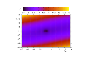
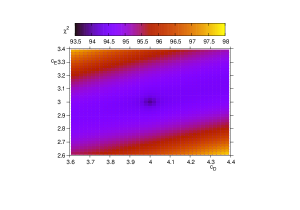
Figure 4: (color online) The maps of $\chi^{2}$ per datum point ($\chi^{2}/N$) values from fitting the pseudo-data at $E=70$ MeV with complete (up) and incomplete (down) theory (see text for explanations).

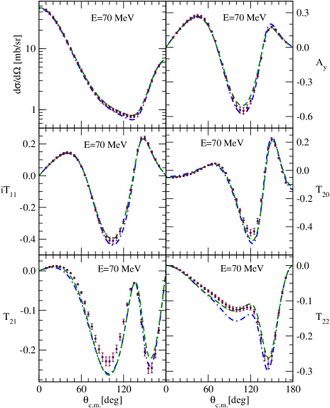
Figure 5: (color online) (left column) The influence of the lacking dynamics on the results of the least-squares fit on the example of pseudo-data ((maroon) circles) for elastic nd scattering differential cross section $\frac{d\sigma}{d\Omega}$ as well as for all the nucleon and deuteron analyzing powers: $A_{y}$, $iT_{11}$, $T_{20}$, $T_{21}$, and $T_{22}$, at $E=70$ MeV. The pseudo-data were generated with our emulator using the SMS N⁴LO⁺ NN potential with the regularization parameter $\Lambda=450$ MeV, supplemented with the N²LO 3NF with the strengths of contact terms $c_{D}=1.0$ and $c_{E}=1.0$. To each data point a relative error of $5\%$ was prescribed. The (blue) dashed-dotted line is the result of 3N calculations with the above-defined dynamics but omitting the parameter free 2$\pi$-exchange N²LO 3NF term. The (green) dashed line is the result of the least-squares fit to the pseudo-data with this lacking dynamics, which provided values of $c_{D}=3.98\pm 0.08$ and $c_{E}=2.99\pm 0.03$.

When studying that point we took a step further and investigated the situation in which the data are fitted with an incomplete theory, that is when some parts of the underlying dynamics are missing. Evidently such a situation occurs when we try to fix strengths of short-range contact terms without the N³LO 3NF components included in the calculations. To study such a case we generated similarly as previously pseudo-data at $E=70$ MeV taking chiral dynamics based on N⁴LO⁺ NN SMS interaction supplemented by the complete N²LO 3NF with strengths of the D and E terms $c_{D}=c_{E}=1.0$. To such pseudo-data we performed a least-squares fit in order to fix strengths $c_{D}$ and $c_{E}$, using original dynamics, omitting however parameter-free $2\pi$-exchange term in the N²LO 3NF. The results are shown in Fig.4 in the form of maps of $\chi^{2}$ per datum point values in space of $c_{D}-c_{E}$. With complete dynamics we recovered easily the incorporated strengths and obtained $c_{D}=1.00\pm 0.08$ and $c_{E}=1.00\pm 0.03$, reaching at that point values of $\chi^{2}=0.0$. When the fit was performed with incomplete dynamics we found a significant shift of the $\chi^{2}$ minimum position to larger values of $c_{D}=3.98\pm 0.08$ and $c_{E}=2.99\pm 0.03$, with concurrent deterioration of the quality of data description as evidenced by increased minimal values of $\chi^{2}$ per datum point $\chi^{2}/N\approx 80$ compared to $\chi^{2}/N\approx 0$ for complete dynamics. In Fig.5 we present in more detail the quality of pseudo-data description by showing pseudo-data themselves ((maroon) circles) and predictions obtained with the incomplete dynamics ((blue) dashed-dotted lines). The (green) dashed line is the result of the least-squares fit to the pseudo-data with incomplete dynamics, which, in general, improves slightly description of data but at the expense of increased strengths of short-range terms D and E.

Since the essential element, namely the N³LO components of the chiral 3NF, is missing in our dynamics, in view of above it is evident that results and conclusions of the present investigation have to be treated with caution and this study must be considered as preliminary. It should be repeated when the N³LO 3NF components become available. Nonetheless, having that restriction in mind, we are ready to answer our main question. To this end we prepared Nd elastic scattering data base at the five energies $E=10,70,135,190,$ and $250$ MeV, collecting data points for the differential cross section, the nucleon vector analysing power, and the deuteron vector and tensor analysing powers, which reflects more or less the status of the presently available Nd data and which are listed in Table 2, and performed multi-energy least-squares fit to data at three energies ($E=10,70,$ and $135$ MeV). Since our 3N continuum calculations neglect the proton-proton (pp) Coulomb force, whose effects in elastic pd scattering are restricted mostly to small energies and forward c.m. angles, we took only pd data at $\theta_{c.m.}>40^{\circ}$ when calculating $\chi^{2}$ (altogether $786$ data points).

The resulting values of strengths $c_{i}$ are listed in Table 3 together with errors (standard deviations) obtained from the covariance matrix $C(c_{i},c_{j})$ shown in Table 4. The four strengths which have large magnitudes belong to the subleading order N⁴LO: $c_{E_{1}}=6.40$, $c_{E_{2}}=7.80$, $c_{E_{3}}=6.97$, and $c_{E_{7}}=-7.40$. It is interesting to note that only strengths in this order, mostly those with large magnitude, $c_{E_{1}}$, $c_{E_{2}}$, and $c_{E_{3}}$, are strongly correlated as evidenced by the values of the corresponding correlation coefficients: $\rho(c_{E_{1}},c_{E_{2}})=0.95$, $\rho(c_{E_{1}},c_{E_{3}})=0.98$, $\rho(c_{E_{2}},c_{E_{3}})=0.93$. The strength $c_{E_{3}}$ is also strongly correlated with $c_{E_{4}}$: $\rho(c_{E_{3}},c_{E_{4}})=-0.92$, and $c_{E_{7}}$ with $c_{E_{8}}$: $\rho(c_{E_{7}},c_{E_{8}})=0.99$. There is only a small correlation between $c_{D}$ or $c_{E}$ and all subleading terms as well as between $c_{D}$ and $c_{E}$ themselves. The final value of $\chi^{2}$ per data point $\chi^{2}/N\approx 35$ indicates that the quality of data description is notably inferior than in the case of the nucleon-nucleon system. The large value of final $\chi^{2}/N$ as well as large magnitudes of some strengths probably reflect the omission of the N³LO term in the 3NF. Therefore the present investigation should be repeated when this term is available.

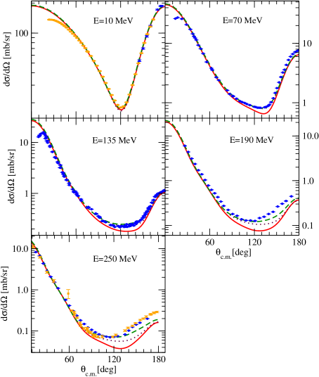
Figure 6: (color online) The elastic Nd scattering differential cross section $\frac{d\sigma}{d\Omega}$ at the incoming nucleon laboratory energies $E=10,70,135,190,$ and $250$ MeV. The (red) solid lines were obtained with the SMS N⁴LO⁺ NN potential with the regularization parameter $\Lambda=450$ MeV. When that potential is supplemented with the N²LO 3NF with the strengths of the contact terms $c_{d}=2.0$ and $c_{E}=0.2866$ (combination reproducing the ³H binding energy and providing a good description of the $70$ MeV pd cross sections) predictions are displyed with the (maroon) dotted lines. The (green) dashed lines show the results obtained with the strengths of contact terms presented in Table 3, fixed in the multi-energy least-squares fit to data at $E=10,70,$ and $135$ MeV (shown in Table 2). The (blue) circles and (orange) squares are $10$ MeV nd data from [38] and pd data from [39], respectively, The (blue) circles at other energies are pd data from: $70$ MeV [43], $135$ MeV [43, 45], $190$ MeV [46], $250$ MeV [50]. The (orange) squares at $250$ MeV are $248$ MeV nd data of [49].

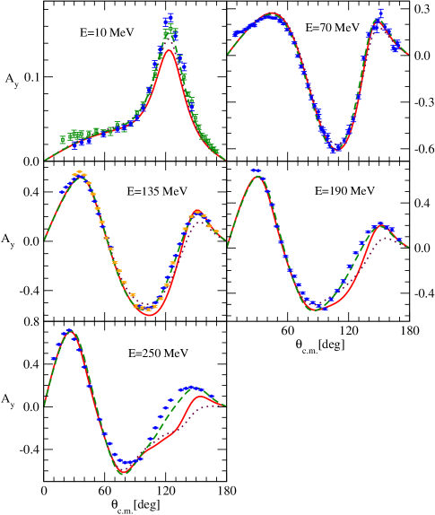
Figure 7: (color online) The same as in Fig.6 but for the nucleon analyzing power $A_{y}$. The data are from: $10$ MeV (blue) circles nd data [40] and (green) squares pd data [41], $70$ MeV (blue) circles pd data (at $65$ MeV) [44], $135$ MeV (blue) circles pd data [47] (orange) squares pd data [46], $190$ MeV (blue) circles pd data [46], $250$ MeV (blue) circles pd data [50].

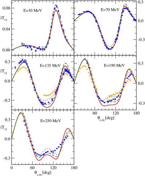
Figure 8: (color online) The same as in Fig.6 but for the deuteron vector analyzing power $iT_{11}$. The data are from: $10$ MeV (blue) circles pd data [42, 41], $70$ MeV (blue) circles pd data [43], $135$ MeV (blue) circles pd data [47] (orange) squares pd data [46], $190$ MeV (blue) circles pd data [48] (orange) squares pd data (at $200$ MeV) [47], $250$ MeV (blue) circles pd data [50].

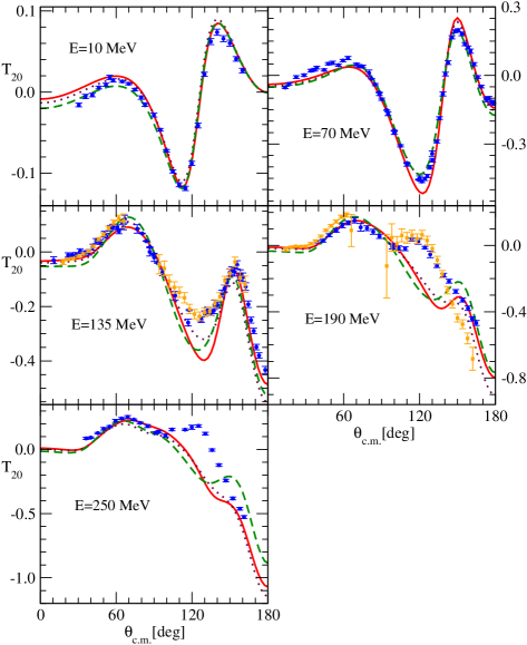
Figure 9: (color online) The same as in Fig.6 but for the deuteron tensor analyzing power $T_{20}$. The data are from: $10$ MeV (blue) circles pd data [41], $70$ MeV (blue) circles pd data [43], $135$ MeV (blue) circles pd data [48] (orange) squares pd data [47], $190$ MeV (blue) circles pd data [48] (orange) squares pd data (at $200$ MeV) [47], $250$ MeV (blue) circles pd data [51].

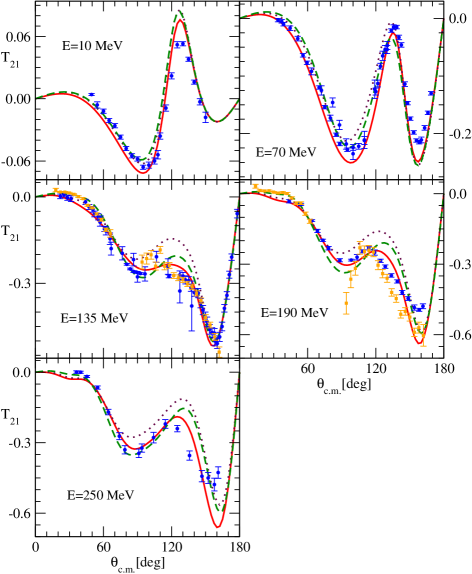
Figure 10: (color online) The same as in Fig.6 but for the deuteron tensor analyzing power $T_{21}$. The data are from: $10$ MeV (blue) circles pd data [41], $70$ MeV (blue) circles pd data [43], $135$ MeV (blue) circles pd data [48] (orange) squares pd data [47], $190$ MeV (blue) circles pd data [48] (orange) squares pd data (at $200$ MeV) [47], $250$ MeV (blue) circles pd data [51].

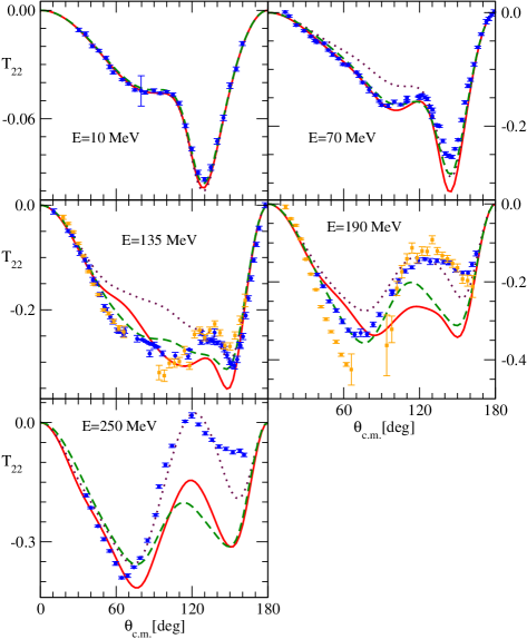
Figure 11: (color online) The same as in Fig.6 but for the deuteron tensor analyzing power $T_{22}$. The data are from: $10$ MeV (blue) circles pd data [41], $70$ MeV (blue) circles pd data [43], $135$ MeV (blue) circles pd data [43] (orange) squares pd data [47], $190$ MeV (blue) circles pd data [48] (orange) squares pd data (at $200$ MeV) [47], $250$ MeV (blue) circles pd data [51].

In Figs.6-11 we show how well the data from our basis (the (green) dashed lines) are described by the 3N Hamiltonian with fixed in this way strengths of contact terms. Since the least-squares fit was performed for data at 3 lowest energies the results at $190$ and $250$ MeV should be considered as predictions. To asses the magnitudes of the contact terms’ effects we show also predictions based on the NN SMS N⁴LO⁺ potential (the (red) solid lines) and the results obtained when the latter was augmented by the N²LO 3NF with the strengths of D and E terms, $c_{D}=2.0$, $c_{E}=0.2866$, determined from the ³H binding energy and the $70$ MeV pd cross section (the (maroon) dotted lines).

In nearly all cases the fit to data improves significantly the description of not only fitted data but also the data at the two largest energies. It is very clear, especially for the cross section (see Fig.6), where the discrepancy between data and theory, found in the region of the cross section minimum up to the backward c.m. angles, is practically removed at $70$ and $135$ MeV. At $190$ and $250$ MeV the inclusion of N⁴LO contact terms brings the theory closer to data.

For the nucleon $A_{y}$ and the deuteron vector $iT_{11}$ analyzing powers there is a significant improvement of the data description in the maximum of the analyzing power at $10$ MeV (see Figs.7 and 8). That effect was also found below the deuteron breakup threshold in Ref. [26] and supports the conclusion of  [26] that the low energy analyzing power puzzle may probably find its solution in the subleading N⁴LO 3NF contact terms.

A similar picture emerges for the tensor analysing powers (see Figs.9-11); here, however, at the largest energies big discrepancies to data remain.

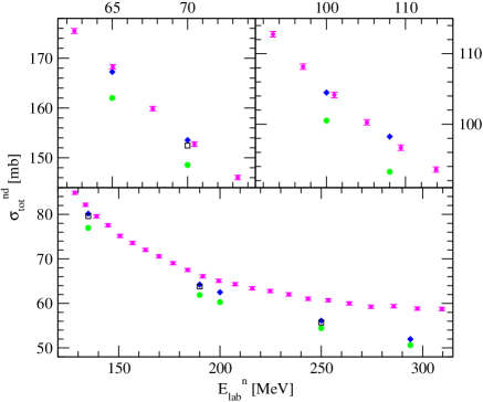
Figure 12: (color online) The total cross section for neutron-deuteron scattering. The (green) circles are predictions of the SMS N⁴LO⁺ NN potential with the regularization parameter $\Lambda=450$ MeV. That potential supplemented by N²LO 3NF with strengths $c_{D}=2.0$ and $c_{E}=0.2866$ gives (blue) diamonds (combination of strengths reproducing the ³H binding energy and the $70$ MeV pd cross section data). The (green) squares are the total nd cross sections obtained with the strengths of N²LO and N⁴LO contact terms fixed in the multi-energy ($E=10,70,$ and $135$ MeV) least-squares fit to Nd data, shown in Table 3. The (magenta) circles are the nd data from [6].

The large advancement in the description of the elastic Nd scattering cross section documented in Fig.6 at the two largest energies prompted us to verify the situation for the total nd scattering cross section. In Fig.12 we show at a few energies the SMS N⁴LO⁺ NN potential predictions (the (green) circles) together with results calculated with this NN force combined with the N²LO 3NF ((blue) diamonds). We display also the total cross section data from Ref. [6] ((magenta) circles). Additionally the total cross sections obtained with the contact terms fixed by the least-squares fit ((green) squares) are shown at the selected four energies. Up to $135$ MeV the inclusion of the 3NF (N²LO or N²LO combined with contact N⁴LO terms) agrees with the total cross section data. However, at $190$ and $250$ MeV even the addition of N⁴LO contact terms, what significantly improved the description of the elastic Nd scattering cross section, does not help to remove the growing with energy gap between data and theory. It means that very likely 3NF is not responsible for that discrepancy. Since at these energies pion production starts to play a role, it is very probably that this new channel, not taken into account in our purely nucleonic scheme, is responsible for this discrepancy.

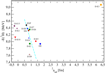
Figure 13: (color online) The doublet nd scattering length ${}^{2}a_{nd}$ and the triton binding energy $E_{{}^{3}H}$ (in 18 channel calculations ($j_{max}=2$)) for different combinations of 2N and/or 3N forces. The (red) circle is the result for the SMS N⁴LO⁺ NN potential with the regularization parameter $\Lambda=450$ MeV. Other symbols show results for that NN potential combined with the N²LO 3NF and supplemented by a sum of the consecutive N⁴LO contact terms (all contact terms with strengths from Table 3: (blue) circle (DE) - D+E N${}^{2}LO$, (green) square (D-E1=D+E+E1), (maroon) plus (D-E2=D+E+E1+E2), (blue) plus (D-E4), (red) diamond (D-E5), (green) square (D-E6), (black) x (D-E7), (blue) diamond (D-E8), (brown) triangle up (D-E9), (red) triangle down (D-E10), (maroon) triangle left (D-E13). The (cyan) dashed line is a Phillips line for (semi)phenomenological interactions from Ref. [52]. The (black) diamond shows the experimental values of ${}^{2}a_{nd}=0.645\pm 0.003$ fm  [53] and $E_{{}^{3}H}=-8.4820(1)$ MeV.

In investigations of the 3N continuum performed up to now with chiral forces, only N²LO components of a 3NF were included and the experimental triton binding energy was essential for determining the low energy constants $c_{D}$ and $c_{E}$, by providing a set of pairs ($c_{D}$,$c_{E}$) which reproduced that basic quantity (forming the so-called “correlation line” [22, 23, 27]). In this way it was ensured that the triton energy is correctly reproduced. Since the doublet nd scattering length ${}^{2}a_{nd}$ is strongly correlated with the triton binding energy $E_{{}^{3}H}$ (often displayed in the form of the so-called Phillips line [52]), it assures also a more or less correct description of this quantity. In Fig.13 we show predictions for the triton binding energy and for the doublet scattering length ${}^{2}a_{nd}$ obtained with the 3N Hamiltonian based on the SMS N⁴LO⁺ NN potential combined with N²LO 3NF together with all the subleading N⁴LO contact terms with the values of strengths of the short-range components from Table 3 ((D-E13 maroon) triangle left). We show also results for $E_{{}^{3}H}$ and ${}^{2}a_{nd}$ obtained by consecutive addition, to 2$\pi$-exchange term, of contact terms, starting from N²LO 3NF (only $D$ and $E$ terms added: $DE$) and terminating when all the N⁴LO contact terms are added ($D+E+E_{1}+\dots E_{13}$: $DE_{13}$). We display also the result for the SMS N⁴LO⁺ NN potential ((NN red) circle) and the Phillips line  [52], along which predictions for $E_{{}^{3}H}$ and ${}^{2}a_{nd}$ of (semi)phenomenological NN potentials, alone or combined with standard 3NF’s, congregate. We observe large scattering of predictions around Phillips line for different combinations of the contact terms. Especially large deviation from the Phillips line occurs when contact terms up to $E_{3}$ are added, leading to $E_{{}^{3}H}$ and ${}^{2}a_{nd}$ which are far away from the experimental values ($E^{exp}_{{}^{3}H}=-8.4820(1)$ MeV and ${}^{2}a^{exp}_{nd}=0.645\pm 0.03$ fm  [53]). It is evident that our 3N Hamiltonian is not able to reproduce the experimental values of the triton binding energy and the doublet ${}^{2}a_{nd}$ scattering length. It seems that the strategy for determining the low energy constants applied when only N²LO 3NF is included in 3N calculations, needs to be modified when N⁴LO short-range terms are also present. One has to forgo the correlation line and incorporate the experimental triton binding energy in the fitting procedure in a different way. One possibility would be to include ${}^{2}a_{nd}$ in the fit using the same approach as for the scattering, what by means of the Phillips line would probably provide the correct binding energy of ³H. Of course, with the availability of the N³LO 3NF part it should be checked how far the description of $E_{{}^{3}H}$ and ${}^{2}a_{nd}$ will be changed by a new set of determined strengths.

V Summary and conclusions

In this paper we investigate the significance of the chiral 3NF contact terms for the description of the Nd elastic scattering observables for the incoming nucleon energies up to the pion production threshold. We used the high precision SMS N⁴LO⁺ NN potential of Ref. [16] in combination with the N²LO chiral 3NF supplemented by all the N⁴LO contact terms. Our aim was to verify if it would be possible to fix strengths of all the contact terms by performing the least-squares fit of theory to Nd elastic scattering data.

The main results are summarized as follows.

• In addition to the two contact terms of the N²LO 3NF there are thirteen contact terms in the N⁴LO 3NF, with two pairs being fully equivalent. Therefore a 3N Hamiltonian depends altogether on 13 parameters which are the strengths of those contact terms. They have to be found by fitting theoretical predictions to 3N data. We found out that the pattern of sensitivities for elastic Nd scattering observables to these 3NF components is diversified and changes with energy, observable and contact terms themselves. This provides a good base to fix the strengths of all the contact terms by fitting theoretical predictions to Nd data. It should be emphasised that even at lower energies the N²LO contact terms are not the most essential and all the short range terms contribute equally.

• Using pseudo-data for the cross section and for a complete set of nucleon and deuteron analyzing powers, generated with our emulator, we checked that indeed it is possible to extract with high precision strengths of all the contact terms by the least-squares fit of theoretical predictions to such pseudo-data. Restricting to N²LO 3NF only and neglecting parameter-free $2\pi$-exchange term in the 3NF we discovered implications of the missing dynamics on the results of such a procedure. There is a significant shift of determined strengths with concurrent deterioration of the quality of data description.

• Taking available Nd data for the cross section and a complete set of nucleon and deuteron analyzing powers at $10,70,$ and $135$ MeV, we fixed strengths of all the contact terms by performing a least-squares fit to these data. With a 3N Hamiltonian defined in this way we received not only a more satisfactory description of the fitted data but for most cases also an improved description of the data taken at $190$ and $250$ MeV. Among others, we found a significant improvement of the description for the low-energy analyzing power $A_{y}$ and $iT_{11}$ as well as for the cross section at higher energies in the region around its minimum up to the backward angles. However, the large gap between the theory and data for the total nd cross section at energies above $\approx 200$ MeV remains, showing that it is not due to missing components of 3NF but results probably from opening a new channel with real pion production.

• We found that the improved description of Nd elastic scattering data does not lead simultaneously to a good description of the triton binding energy and the doublet nd scattering length ${}^{2}a_{nd}$. Especially the scattering length obtained with fixed strengths of the contact terms lies far away from its experimental value. It will be interesting to see if inclusion of N³LO 3NF component will improve the description of these two quantities.

It should be stressed out that in our dynamics the N³LO 3NF component is missing. Therefore one should take the determined values of the strengths with some caution. From the theoretical side, efforts to include in the 3N continuum calculations consistently regularized N³LO 3NF components are required what is the aim of the LENPIC collaboration. When such N³LO 3NF becomes available the present study will be repeated.

The elastic Nd scattering observables are driven by the S-matrix; therefore they are predominantly sensitive to the potential energy of three nucleons, whose main part is given by the pairwise interactions. Contrary to that, the nuclear bound states are sensitive to the interplay between the kinetic and potential energies of nucleons, being thus more sensitive to 3NF’s. Based on the presented results it seems very probable that N⁴LO contact terms will have also large influence on spectra of nuclei. Therefore it would be interesting to apply the nuclear Hamiltonian proposed in the present paper to bound nuclear systems and see what effects the N⁴LO contact terms have on the energy spectra and other properties of nuclei.

Appendix A Momentum space partial wave decomposition of the N⁴LO 3NF contact terms

Here we introduce our definitions of the Faddeev components corresponding to all the different N⁴LO 3NF contact terms: $E_{2},E_{3},E_{4},E_{5},E_{6},E_{8},E_{9},E_{10},$ and $E_{11}$. Then we provide their momentum-space partial wave decomposition in the basis $|p~{}q~{}\alpha>$. In the following $\vec{p}$ and $\vec{q}$ ($\vec{p}~{}^{\prime}$ and $\vec{q}~{}^{\prime}$) denote the relative initial (final) Jacobi momenta. The other vectors, $\vec{q}_{i}=\vec{p}_{i}~{}^{\prime}-\vec{p}_{i}$ and $\vec{K}_{i}=\frac{\vec{p}_{i}~{}^{\prime}+\vec{p}_{i}}{2}$, are defined by the individual initial $\vec{p}_{i}$ (final $\vec{p}_{i}~{}^{\prime}$) nucleon momenta ($i=1,2,3$).

The partial wave decomposition for the $E_{1}$ and $E_{7}$ terms can be found in [27]. For details on our notation we refer the reader to Ref. [1]. In particular we use $\hat{X}\equiv 2X+1$, where $X$ is an integer or a half-integer.

For the E₂-term

$$V_{3N} = E_{2}\sum_{i\neq j\neq k}\vec{q_{i}}^{2}\vec{\tau}_{i}\cdot\vec{\tau}_{j}$$ (31)

we define the Faddeev component as

$$V_{3N}^{(1)} = E_{2}\vec{q_{1}}^{2}(\vec{\tau}_{1}\cdot\vec{\tau}_{2}+\vec{\tau}_{1}\cdot\vec{\tau}_{3})$$ (32)

and arrive at the following matrix elements:

$$<p^{\prime}~{}q^{\prime}~{}\alpha^{\prime}|V_{3N}^{(1)}|p~{}q~{}\alpha> = \frac{1}{4\pi^{4}}E_{2}\delta_{s^{\prime}s}\delta_{l^{\prime}0}\delta_{l0}\delta_{sj^{\prime}}\delta_{sj}\delta_{T^{\prime}T}\delta_{M_{T^{\prime}}M_{T}}\delta_{t^{\prime}t}$$ (35)

$$\times[(q^{2}+q^{\prime 2})\delta_{\lambda^{\prime}0}\delta_{\lambda 0}\delta_{I^{\prime}\frac{1}{2}}\delta_{I\frac{1}{2}}-\frac{2}{3}qq^{\prime}\delta_{\lambda^{\prime}1}\delta_{\lambda 1}\delta_{I^{\prime}I}]$$

$$\times[-12\sqrt{\hat{t}\hat{t}^{\prime}}(-1)^{T-\frac{1}{2}}\begin{Bmatrix}t^{\prime}&t&1\\ \frac{1}{2}&\frac{1}{2}&T\end{Bmatrix}\begin{Bmatrix}t^{\prime}&t&1\\ \frac{1}{2}&\frac{1}{2}&\frac{1}{2}\end{Bmatrix}]~{}.$$

For the E₃-term

$$V_{3N} = E_{3}\sum_{i\neq j\neq k}\vec{q_{i}}^{2}\vec{\sigma}_{1}`\cdot\vec{\sigma}_{j}$$ (36)

we choose the Faddeev component as

$$V_{3N}^{(1)} = E_{3}\vec{q_{1}}^{2}(\vec{\sigma}_{i}\cdot\vec{\sigma}_{2}+\vec{\sigma}_{1}\cdot\vec{\sigma}_{3})$$ (37)

and obtain:

$$<p^{\prime}~{}q^{\prime}~{}\alpha^{\prime}|V_{3N}^{(1)}|p~{}q~{}\alpha> = -\frac{1}{2\pi^{4}}6E_{3}\delta_{s^{\prime}s}\delta_{l^{\prime}0}\delta_{l0}\delta_{sj^{\prime}}\delta_{sj}\delta_{T^{\prime}T}\delta_{M_{T^{\prime}}M_{T}}\delta_{t^{\prime}t}$$ (38)

$$\times(-1)^{J-\frac{1}{2}}\hat{s}\begin{Bmatrix}s&s&1\\ \frac{1}{2}&\frac{1}{2}&\frac{1}{2}\end{Bmatrix} [ (q^{2}+q^{\prime 2})\delta_{\lambda^{\prime}0}\delta_{\lambda 0}\delta_{I^{\prime}\frac{1}{2}}\delta_{I\frac{1}{2}}\begin{Bmatrix}s&s&1\\ \frac{1}{2}&\frac{1}{2}&J\end{Bmatrix}$$ (39)

$$-\frac{2}{3}qq^{\prime}\delta_{\lambda^{\prime}1}\delta_{\lambda 1}\sqrt{\hat{I}\hat{I}^{\prime}} \begin{Bmatrix}1&I^{\prime}&I\\ J&j&j^{\prime}\end{Bmatrix}\begin{Bmatrix}1&I^{\prime}&I\\ 1&\frac{1}{2}&\frac{1}{2}\end{Bmatrix}]~{}.$$ (40)

For the E₄-term

$$V_{3N} = E_{4}\sum_{i\neq j\neq k}\vec{q_{i}}^{2}\vec{\sigma}_{i}\cdot\vec{\sigma}_{j}\vec{\tau}_{i}\cdot\vec{\tau}_{j}$$ (41)

we choose the Faddeev component in the following form:

$$V_{3N}^{(1)} = E_{4}\vec{q_{1}}^{2}(\vec{\sigma}_{1}\cdot\vec{\sigma}_{2}\vec{\tau}_{1}\cdot\vec{\tau}_{2}+\vec{\sigma}_{1}\cdot\vec{\sigma}_{3}\vec{\tau}_{1}\cdot\vec{\tau}_{3})$$ (42)

and obtain

$$<p^{\prime}~{}q^{\prime}~{}\alpha^{\prime}|V_{3N}^{(1)}|p~{}q~{}\alpha> = -\frac{1}{2\pi^{4}}E_{4}36\sqrt{\hat{s}\hat{s}^{\prime}}\begin{Bmatrix}s^{\prime}&s&1\\ \frac{1}{2}&\frac{1}{2}&\frac{1}{2}\end{Bmatrix}\times(-1)^{J+\frac{1}{2}}$$ (43)

$$(-1)^{T^{\prime}-\frac{1}{2}} \sqrt{\hat{t}\hat{t}^{\prime}}\begin{Bmatrix}t^{\prime}&t&1\\ \frac{1}{2}&\frac{1}{2}&T\end{Bmatrix}\begin{Bmatrix}t^{\prime}&t&1\\ \frac{1}{2}&\frac{1}{2}&\frac{1}{2}\end{Bmatrix}\delta_{ll^{\prime}}\delta_{l^{\prime}0}\delta_{l0}\delta_{sj^{\prime}}\delta_{sj}\delta_{T^{\prime}T}\delta_{M_{T^{\prime}}M_{T}}$$ (46)

$$\times[(q^{2}+q^{\prime 2})\delta_{\lambda^{\prime}0}\delta_{\lambda 0}\delta_{I^{\prime}\frac{1}{2}}\delta_{I\frac{1}{2}}\begin{Bmatrix}s^{\prime}&s&1\\ \frac{1}{2}&\frac{1}{2}&J\end{Bmatrix}$$

$$-\frac{2}{3}qq^{\prime}\delta_{\lambda^{\prime}1}\delta_{\lambda 1}\sqrt{\hat{I}^{\prime}\hat{I}}(-1)^{s^{\prime}+s}\begin{Bmatrix}I^{\prime}&1&I\\ \frac{1}{2}&1&\frac{1}{2}\end{Bmatrix}\begin{Bmatrix}I^{\prime}&1&I\\ j&J&j^{\prime}\end{Bmatrix}]~{}.$$

For the E₅-term

$$V_{3N} = E_{5}\sum_{i\neq j\neq k}(3\vec{q}_{i}\cdot\vec{\sigma}_{i}\vec{q}_{i}\cdot\vec{\sigma}_{j}-\vec{q_{i}}^{2}\vec{\sigma}_{i}\cdot\vec{\sigma}_{j})$$ (47)

our definition of the Faddeev component is

$$V_{3N}^{(1)} = E_{5}[3\vec{q_{1}}\cdot\vec{\sigma}_{1}(\vec{q_{1}}\cdot\vec{\sigma}_{2}+\vec{q_{1}}\cdot\vec{\sigma}_{3})-\vec{q_{1}}^{2}(\vec{\sigma}_{1}\cdot\vec{\sigma}_{2}+\vec{\sigma}_{1}\cdot\vec{\sigma}_{3})]$$ (48)

and we get:

$$<p^{\prime}~{}q^{\prime}~{}\alpha^{\prime}|V_{3N}^{(1)}|p~{}q~{}\alpha> = \frac{1}{2\pi^{4}}E_{5}6\sqrt{\hat{s}\hat{s}^{\prime}}\begin{Bmatrix}s^{\prime}&s&1\\ \frac{1}{2}&\frac{1}{2}&\frac{1}{2}\end{Bmatrix}\delta_{l^{\prime}0}\delta_{l0}\delta_{j^{\prime}s^{\prime}}\delta_{js}\delta_{s^{\prime}s}\delta_{tt^{\prime}}\delta_{T^{\prime}T}\delta_{M_{T^{\prime}}M_{T}}$$ (49)

$$\times[3q^{\prime}q^{\prime}\sqrt{\frac{\hat{I}^{\prime}}{\hat{J}}}(-1)^{j^{\prime}+I^{\prime}+s}\delta_{\lambda 0}\delta_{I\frac{1}{2}} <1010|\lambda^{\prime}0>\sum_{S^{\prime}}{\hat{S}^{\prime}\sqrt{\hat{S}^{\prime}}(-1)^{S^{\prime}}\begin{Bmatrix}J&I^{\prime}&j^{\prime}\\ \frac{1}{2}&S^{\prime}&\lambda^{\prime}\end{Bmatrix}\begin{Bmatrix}S^{\prime}&J&\lambda^{\prime}\\ s^{\prime}&s&1\\ \frac{1}{2}&\frac{1}{2}&1\end{Bmatrix}}$$ (50)

$$+3qq\sqrt{{\hat{I}}{\hat{J}}}(-1)^{j+I+s^{\prime}}\delta_{\lambda^{\prime}0}\delta_{I^{\prime}\frac{1}{2}} <1010|\lambda 0>\sum_{S}\sqrt{{\hat{S}}}(-1)^{S}\begin{Bmatrix}J&I&j\\ \frac{1}{2}&S&\lambda\end{Bmatrix}\begin{Bmatrix}S&J&\lambda\\ s&s^{\prime}&1\\ \frac{1}{2}&\frac{1}{2}&1\end{Bmatrix}$$ (51)

$$-2q^{\prime}q\sqrt{{\hat{I}}{\hat{I}^{\prime}}}(-1)^{J+\frac{1}{2}+j^{\prime}}\delta_{\lambda^{\prime}1}\delta_{\lambda 1} \begin{Bmatrix}I^{\prime}&1&I\\ \frac{1}{2}&1&\frac{1}{2}\end{Bmatrix}\begin{Bmatrix}I^{\prime}&1&I\\ j&J&j^{\prime}\end{Bmatrix}$$ (54)

$$+(-1)^{J+\frac{1}{2}}\{(q^{2}+q^{\prime 2})\delta_{\lambda^{\prime}0}\delta_{\lambda 0}\delta_{I^{\prime}\frac{1}{2}}\delta_{I\frac{1}{2}}\begin{Bmatrix}s^{\prime}&s&1\\ \frac{1}{2}&\frac{1}{2}&J\end{Bmatrix}$$

$$-\frac{2}{3}qq^{\prime}\delta_{\lambda^{\prime}1}\delta_{\lambda 1}\sqrt{\hat{I}^{\prime}\hat{I}}\begin{Bmatrix}I^{\prime}&1&I\\ \frac{1}{2}&1&\frac{1}{2}\end{Bmatrix}\begin{Bmatrix}I^{\prime}&1&I\\ j&J&j^{\prime}\end{Bmatrix}\}]~{}.$$

For the E₆-term

$$V_{3N} = E_{6}\sum_{i\neq j\neq k}(3\vec{q}_{i}\cdot\vec{\sigma}_{i}\vec{q}_{i}\cdot\vec{\sigma}_{j}-\vec{q_{i}}^{2}\vec{\sigma}_{i}\cdot\vec{\sigma}_{j})\vec{\tau}_{i}\cdot\vec{\tau}_{j}$$ (55)

our choice of the Faddeev component reads

$$V_{3N}^{(1)} = E_{6}[(3\vec{q_{1}}\cdot\vec{\sigma}_{1}\vec{q_{1}}\cdot\vec{\sigma}_{2}-\vec{q_{1}}^{2}\vec{\sigma}_{1}\cdot\vec{\sigma}_{2})\vec{\tau}_{1}\cdot\vec{\tau}_{2}$$ (57)

$$+(3\vec{q_{1}}\cdot\vec{\sigma}_{1}\vec{q_{1}}\cdot\vec{\sigma}_{3}-\vec{q_{1}}^{2}\vec{\sigma}_{1}\cdot\vec{\sigma}_{3})\vec{\tau}_{1}\cdot\vec{\tau}_{3}]$$

and we get:

$$<p^{\prime}~{}q^{\prime}~{}\alpha^{\prime}|V_{3N}^{(1)}|p~{}q~{}\alpha> = -\frac{1}{2\pi^{4}}E_{6}36\sqrt{\hat{j}\hat{j}^{\prime}}\begin{Bmatrix}j^{\prime}&j&1\\ \frac{1}{2}&\frac{1}{2}&\frac{1}{2}\end{Bmatrix}\delta_{ll^{\prime}}\delta_{l^{\prime}0}\delta_{l0}\delta_{s^{\prime}j^{\prime}}\delta_{sj}$$ (58)

$$\times[3q^{\prime}q^{\prime}\sqrt{\frac{\hat{I}^{\prime}}{\hat{J}}}(-1)^{j^{\prime}+j+I^{\prime}}\delta_{\lambda 0}\delta_{I\frac{1}{2}} <1010|\lambda^{\prime}0>\sum_{S^{\prime}}{\hat{S}^{\prime}\sqrt{\hat{S}^{\prime}}(-1)^{S^{\prime}}\begin{Bmatrix}J&I^{\prime}&j^{\prime}\\ \frac{1}{2}&S^{\prime}&\lambda^{\prime}\end{Bmatrix}\begin{Bmatrix}S^{\prime}&J&\lambda^{\prime}\\ \frac{1}{2}&\frac{1}{2}&1\end{Bmatrix}}$$ (59)

$$+3qq\sqrt{{\hat{I}}{\hat{J}}}(-1)^{j^{\prime}+j+I}\delta_{\lambda^{\prime}0}\delta_{I^{\prime}\frac{1}{2}} <1010|\lambda 0>\sum_{S}{\sqrt{\hat{S}}(-1)^{S}\begin{Bmatrix}J&I&j\\ \frac{1}{2}&S&\lambda\end{Bmatrix}\begin{Bmatrix}S&J&\lambda\\ s&s^{\prime}&1\\ \frac{1}{2}&\frac{1}{2}&1\end{Bmatrix}}$$ (60)

$$-2q^{\prime}q\sqrt{{\hat{I}}{\hat{I}^{\prime}}}(-1)^{J+\frac{1}{2}+j^{\prime}}\delta_{\lambda^{\prime}1}\delta_{\lambda 1} \begin{Bmatrix}I^{\prime}&1&I\\ \frac{1}{2}&1&\frac{1}{2}\end{Bmatrix}\begin{Bmatrix}I^{\prime}&1&I\\ j&J&j^{\prime}\end{Bmatrix}$$ (61)

$$-(-1)^{J+\frac{1}{2}} \{(q^{2}+q^{\prime 2})\delta_{\lambda^{\prime}0}\delta_{\lambda 0}\delta_{I^{\prime}\frac{1}{2}}\delta_{I\frac{1}{2}}\begin{Bmatrix}s^{\prime}&s&1\\ \frac{1}{2}&\frac{1}{2}&J\end{Bmatrix}$$ (62)

$$-\frac{2}{3}qq^{\prime}\delta_{\lambda^{\prime}1}\delta_{\lambda 1}\sqrt{\hat{I}^{\prime}\hat{I}} (-1)^{j+j^{\prime}}\begin{Bmatrix}I^{\prime}&1&I\\ \frac{1}{2}&1&\frac{1}{2}\end{Bmatrix}\begin{Bmatrix}I^{\prime}&1&I\\ j&J&j^{\prime}\end{Bmatrix}\}]$$ (63)

$$\times[\delta_{T^{\prime}T}\delta_{M_{T^{\prime}}M_{T}}\sqrt{\hat{t}\hat{t}^{\prime}} (-1)^{T^{\prime}-\frac{1}{2}}\begin{Bmatrix}t^{\prime}&t&1\\ \frac{1}{2}&\frac{1}{2}&T\end{Bmatrix}\begin{Bmatrix}t^{\prime}&t&1\\ \frac{1}{2}&\frac{1}{2}&1\end{Bmatrix}]~{}.$$ (64)

For the E₈-term

$$V_{3N} = iE_{8}\sum_{i\neq j\neq k}\vec{q_{i}}\times(\vec{K}_{i}-\vec{K}_{j})\cdot(\vec{\sigma}_{i}+\vec{\sigma}_{j})\vec{\tau}_{j}\cdot\vec{\tau}_{k}$$ (65)

we choose the Faddeev component as

$$V_{3N}^{(1)} = iE_{8}[\vec{q_{1}}\times(\vec{K}_{1}-\vec{K}_{2})\cdot(\vec{\sigma}_{1}+\vec{\sigma}_{2})\vec{\tau}_{2}\cdot\vec{\tau}_{3}+\vec{q_{1}}\times(\vec{K}_{1}-\vec{K}_{3})\cdot(\vec{\sigma}_{1}+\vec{\sigma}_{3})\vec{\tau}_{3}\cdot\vec{\tau}_{2}]$$ (66)

and get:

$$<p^{\prime}~{}q^{\prime}~{}\alpha^{\prime}|V_{3N}^{(1)}|p~{}q~{}\alpha> = -\frac{1}{8\pi^{4}}E_{8}\delta_{T^{\prime}T}\delta_{M_{T^{\prime}}M_{T}}\delta_{t^{\prime}t}6(-1)^{t}\begin{Bmatrix}\frac{1}{2}&\frac{1}{2}&1\\ \frac{1}{2}&\frac{1}{2}&t\end{Bmatrix}$$ (74)

$$\times[\,-\sqrt{2}(1-(-1)^{s^{\prime}+s})(-1)^{J+\frac{1}{2}}$$

$$\times(\,~{}qp\delta_{l^{\prime}0}\delta_{\lambda^{\prime}0}\delta_{l1}\delta_{\lambda 1}\delta_{s^{\prime}j^{\prime}}\delta_{I^{\prime}\frac{1}{2}}\sqrt{\hat{j}\hat{I}}\begin{Bmatrix}1&s&s^{\prime}\\ j&1&1\end{Bmatrix}\begin{Bmatrix}s^{\prime}&j&1\\ I&\frac{1}{2}&J\end{Bmatrix}$$

$$~{}-qp^{\prime}\delta_{l^{\prime}1}\delta_{\lambda^{\prime}0}\delta_{l0}\delta_{\lambda 1}\delta_{sj}\delta_{I^{\prime}\frac{1}{2}}\sqrt{\hat{j}^{\prime}\hat{I}}\begin{Bmatrix}1&s^{\prime}&s\\ j^{\prime}&1&1\end{Bmatrix}\begin{Bmatrix}j^{\prime}&s&1\\ I&\frac{1}{2}&J\end{Bmatrix}$$

$$~{}-q^{\prime}p\delta_{l^{\prime}0}\delta_{\lambda^{\prime}1}\delta_{l1}\delta_{\lambda 0}\delta_{s^{\prime}j^{\prime}}\delta_{I\frac{1}{2}}\sqrt{\hat{j}\hat{I}^{\prime}}\begin{Bmatrix}1&s&s^{\prime}\\ j&1&1\end{Bmatrix}\begin{Bmatrix}j&s^{\prime}&1\\ I^{\prime}&\frac{1}{2}&J\end{Bmatrix}$$

$$~{}+q^{\prime}p^{\prime}\delta_{l^{\prime}1}\delta_{\lambda^{\prime}1}\delta_{l0}\delta_{\lambda 0}\delta_{sj}\delta_{I\frac{1}{2}}\sqrt{\hat{j}^{\prime}\hat{I}^{\prime}}\begin{Bmatrix}1&s^{\prime}&s\\ j^{\prime}&1&1\end{Bmatrix}\begin{Bmatrix}s&j^{\prime}&1\\ I^{\prime}&\frac{1}{2}&J\end{Bmatrix})\,$$

$$~{}+12qq^{\prime}\delta_{l^{\prime}0}\delta_{\lambda^{\prime}1}\delta_{l0}\delta_{\lambda 1}\delta_{s^{\prime}s}\delta_{s^{\prime}j^{\prime}}\delta_{sj}(\delta_{I^{\prime}I}(-1)^{I+\frac{1}{2}}\begin{Bmatrix}\frac{1}{2}&1&I\\ 1&\frac{1}{2}&1\end{Bmatrix}$$

$$+\delta_{s1}\sqrt{\hat{I}\hat{I}^{\prime}}(-1)^{I^{\prime}+I+J+\frac{1}{2}}\begin{Bmatrix}1&I&I^{\prime}\\ \frac{1}{2}&1&1\end{Bmatrix}\begin{Bmatrix}1&I&I^{\prime}\\ J&1&1\end{Bmatrix})]\,~{}.$$

For the E₉-term

$$V_{3N} = E_{9}\sum_{i\neq j\neq k}\vec{q}_{i}\cdot\vec{\sigma}_{i}\vec{q}_{j}\cdot\vec{\sigma}_{j}$$ (75)

we define the Faddeev component as

$$V_{3N}^{(1)} = E_{9}[\vec{q_{1}}\cdot\vec{\sigma}_{1}(\vec{q_{2}}\cdot\vec{\sigma}_{2}+\vec{q_{3}}\cdot\vec{\sigma}_{3})]$$ (76)

and get:

$$<p^{\prime}~{}q^{\prime}~{}\alpha^{\prime}|V_{3N}^{(1)}|p~{}q~{}\alpha> = \frac{1}{2\pi^{4}}E_{9}\delta_{tt^{\prime}}\delta_{T^{\prime}T}\delta_{M_{T^{\prime}}M_{T}}\begin{Bmatrix}s^{\prime}&s&1\\ \frac{1}{2}&\frac{1}{2}&\frac{1}{2}\end{Bmatrix}\sqrt{\hat{s}\hat{s}^{\prime}}$$ (77)

$$\times[(\frac{1-(-1)^{s+s^{\prime}}}{2})\{ - \sqrt{2}q^{\prime}p\delta_{l^{\prime}0}\delta_{\lambda^{\prime}1}\delta_{l1}\delta_{\lambda 0}\delta_{j^{\prime}s^{\prime}}\delta_{I\frac{1}{2}}\sqrt{{\hat{j}\hat{I}}{\hat{I}^{\prime}}}(-1)^{j^{\prime}+I^{\prime}+J+s}$$ (78)

$$\sum_{S}{\sqrt{\hat{S}}} \begin{Bmatrix}s&j&1\\ J&S&\frac{1}{2}\end{Bmatrix}\begin{Bmatrix}\frac{1}{2}&s&S\\ J&I^{\prime}&j^{\prime}\end{Bmatrix}\begin{Bmatrix}J&I^{\prime}&j^{\prime}\\ \frac{1}{2}&S&1\end{Bmatrix}$$ (79)

$$- \sqrt{2}qp^{\prime}\delta_{l^{\prime}1}\delta_{\lambda^{\prime}0}\delta_{l0}\delta_{\lambda 1}\delta_{js}\delta_{I^{\prime}\frac{1}{2}}\sqrt{\hat{j}^{\prime}\hat{I}\hat{I}^{\prime}}(-1)^{j+I+J+s^{\prime}}$$ (80)

$$\sum_{S}{\sqrt{\hat{S}}} \begin{Bmatrix}s^{\prime}&j^{\prime}&1\\ J&S&\frac{1}{2}\end{Bmatrix}\begin{Bmatrix}\frac{1}{2}&s&S\\ s^{\prime}&\frac{1}{2}&1\end{Bmatrix}\begin{Bmatrix}J&I&j\\ \frac{1}{2}&S&1\end{Bmatrix}$$ (81)

$$+ 2qp\delta_{l^{\prime}0}\delta_{\lambda^{\prime}0}\delta_{l1}\delta_{\lambda 1}\delta_{j^{\prime}s^{\prime}}\delta_{I^{\prime}\frac{1}{2}}\sqrt{{\hat{j}\hat{I}}{\hat{J}}}(-1)^{I^{\prime}-\frac{1}{2}-J-s}$$ (83)

$$\sum_{L,S}{\hat{L}\sqrt{\hat{S}}(-1)^{L+S}}\begin{Bmatrix}1&s&j\\ 1&\frac{1}{2}&I\\ L&S&J\end{Bmatrix}\begin{Bmatrix}J&S&L\\ s^{\prime}&s&1\\ \frac{1}{2}&\frac{1}{2}&1\end{Bmatrix}$$

$$+ 2q^{\prime}p^{\prime}\delta_{l^{\prime}1}\delta_{\lambda^{\prime}1}\delta_{l0}\delta_{\lambda 0}\delta_{js}\delta_{I\frac{1}{2}}\sqrt{{\hat{j}^{\prime}\hat{I}^{\prime}}}(-1)^{I-\frac{1}{2}-J+s^{\prime}}$$ (84)

$$\sum_{L^{\prime},S^{\prime}}{\hat{L}^{\prime}\hat{S}^{\prime}} (-1)^{L^{\prime}+S^{\prime}}\begin{Bmatrix}1&s^{\prime}&j^{\prime}\\ 1&\frac{1}{2}&I^{\prime}\\ L^{\prime}&S^{\prime}&J\end{Bmatrix}\begin{Bmatrix}J&S^{\prime}&L^{\prime}\\ s&s^{\prime}&1\\ \frac{1}{2}&\frac{1}{2}&1\end{Bmatrix}\}$$ (85)

$$+(\frac{1+(-1)^{s+s^{\prime}}}{2})\{-3q^{\prime}q^{\prime}\delta_{l0}\delta_{l^{\prime}0} \delta_{\lambda 0}\delta_{js}\delta_{j^{\prime}s^{\prime}}\delta_{I\frac{1}{2}}\sqrt{\frac{\hat{I}^{\prime}}{\hat{J}}}(-1)^{j^{\prime}-I^{\prime}+s+1}<1010|\lambda^{\prime}0>$$ (87)

$$\sum_{S^{\prime}}{\hat{S}^{\prime}\sqrt{\hat{S}^{\prime}}(-1)^{S^{\prime}}\begin{Bmatrix}J&I^{\prime}&j^{\prime}\\ \frac{1}{2}&S^{\prime}&\lambda^{\prime}\end{Bmatrix}\begin{Bmatrix}S^{\prime}&J&\lambda^{\prime}\\ s^{\prime}&s&1\\ \frac{1}{2}&\frac{1}{2}&1\end{Bmatrix}}$$

$$-3qq\delta_{l0}\delta_{l^{\prime}0} \delta_{\lambda^{\prime}0}\delta_{js}\delta_{j^{\prime}s^{\prime}}\delta_{I^{\prime}\frac{1}{2}}\sqrt{{\hat{I}}{\hat{J}}}(-1)^{j-I+s^{\prime}+1}<1010|\lambda 0>$$ (89)

$$\sum_{S}{\hat{S}(-1)^{S}\begin{Bmatrix}J&I&j\\ \frac{1}{2}&S&\lambda\end{Bmatrix}\begin{Bmatrix}S&J&\lambda\\ s&s^{\prime}&1\\ \frac{1}{2}&\frac{1}{2}&1\end{Bmatrix}}$$

$$+2q^{\prime}q\delta_{l0}\delta_{l^{\prime}0}\delta_{\lambda 1}\delta_{\lambda^{\prime}1}\delta_{js}\delta_{j^{\prime}s^{\prime}}\sqrt{{\hat{I}}{\hat{I}^{\prime}}}(-1)^{J+\frac{1}{2}+j^{\prime}} \begin{Bmatrix}I^{\prime}&1&I\\ \frac{1}{2}&1&\frac{1}{2}\end{Bmatrix}\begin{Bmatrix}I^{\prime}&1&I\\ j&J&j^{\prime}\end{Bmatrix}\}]~{}.$$ (90)

For the E₁₀-term

$$V_{3N} = E_{10}\sum_{i\neq j\neq k}\vec{q}_{i}\cdot\vec{\sigma}_{i}\vec{q}_{j}\cdot\vec{\sigma}_{j}\vec{\tau}_{i}\cdot\vec{\tau}_{j}$$ (91)

we choose the Faddeev component

$$V_{3N}^{(1)} = E_{10}\vec{q_{1}}\cdot\vec{\sigma}_{1}[\vec{q_{2}}\cdot\vec{\sigma}_{2}\vec{\tau}_{1}\cdot\vec{\tau}_{2}+\vec{q_{3}}\cdot\vec{\sigma}_{3}\vec{\tau}_{1}\cdot\vec{\tau}_{3}]$$ (92)

and get:

$$<p^{\prime}~{}q^{\prime}~{}\alpha^{\prime}|V_{3N}^{(1)}|p~{}q~{}\alpha> = \frac{1}{2\pi^{4}}E_{10}\begin{Bmatrix}s^{\prime}&s&1\\ \frac{1}{2}&\frac{1}{2}&\frac{1}{2}\end{Bmatrix}\sqrt{\hat{s}\hat{s}^{\prime}}$$ (93)

$$\times(-6\delta_{T^{\prime}T}\delta_{M_{T^{\prime}}M_{T}} \sqrt{\hat{t}\hat{t}^{\prime}}(-1)^{T-\frac{1}{2}}\begin{Bmatrix}t^{\prime}&t&1\\ \frac{1}{2}&\frac{1}{2}&T\end{Bmatrix}\begin{Bmatrix}t^{\prime}&t&1\\ \frac{1}{2}&\frac{1}{2}&\frac{1}{2}\end{Bmatrix})$$ (94)

$$\times[(\frac{1-(-1)^{l+l^{\prime}}}{2})\{ - \sqrt{2}q^{\prime}p\delta_{l^{\prime}0}\delta_{\lambda^{\prime}1}\delta_{l1}\delta_{\lambda 0}\delta_{j^{\prime}s^{\prime}}\delta_{I\frac{1}{2}}\sqrt{{\hat{j}\hat{I}}{\hat{I}^{\prime}}}(-1)^{j^{\prime}+I^{\prime}+J+s}$$ (96)

$$\sum_{S}{\sqrt{\hat{S}}\begin{Bmatrix}s&j&1\\ J&S&\frac{1}{2}\end{Bmatrix}\begin{Bmatrix}\frac{1}{2}&s&S\\ s^{\prime}&\frac{1}{2}&1\end{Bmatrix}\begin{Bmatrix}J&I^{\prime}&j^{\prime}\\ \frac{1}{2}&S&1\end{Bmatrix}}$$

$$- \sqrt{2}qp^{\prime}\delta_{l^{\prime}1}\delta_{\lambda^{\prime}0}\delta_{l0}\delta_{\lambda 1}\delta_{js}\delta_{I^{\prime}\frac{1}{2}}\sqrt{\hat{j}^{\prime}\hat{I}\hat{I}^{\prime}}(-1)^{j+I+J+s^{\prime}}$$ (98)

$$\sum_{S}{\sqrt{\hat{S}}\begin{Bmatrix}s^{\prime}&j^{\prime}&1\\ J&S&\frac{1}{2}\end{Bmatrix}\begin{Bmatrix}\frac{1}{2}&s&S\\ s^{\prime}&\frac{1}{2}&1\end{Bmatrix}\begin{Bmatrix}J&I&j\\ \frac{1}{2}&S&1\end{Bmatrix}}$$

$$+ 2qp\delta_{l^{\prime}0}\delta_{\lambda^{\prime}0}\delta_{l1}\delta_{\lambda 1}\delta_{j^{\prime}s^{\prime}}\delta_{I^{\prime}\frac{1}{2}}\sqrt{{\hat{j}\hat{I}}{\hat{J}}}(-1)^{I^{\prime}-\frac{1}{2}-J-s}$$ (100)

$$\sum_{L,S}{\hat{L}\sqrt{\hat{S}}(-1)^{L+S}}\begin{Bmatrix}1&s&j\\ 1&\frac{1}{2}&I\\ L&S&J\end{Bmatrix}\begin{Bmatrix}J&S&L\\ s^{\prime}&s&1\\ \frac{1}{2}&\frac{1}{2}&1\end{Bmatrix}$$

$$+ 2q^{\prime}p^{\prime}\delta_{l^{\prime}1}\delta_{\lambda^{\prime}1}\delta_{l0}\delta_{\lambda 0}\delta_{js}\delta_{I\frac{1}{2}}\sqrt{{\hat{j}^{\prime}\hat{I}^{\prime}}}(-1)^{I-\frac{1}{2}-J+s^{\prime}}$$ (101)

$$\sum_{L^{\prime},S^{\prime}}{\hat{S}^{\prime}\hat{L}^{\prime}} (-1)^{L^{\prime}+S^{\prime}}\begin{Bmatrix}1&s^{\prime}&j^{\prime}\\ 1&\frac{1}{2}&I^{\prime}\\ L^{\prime}&S^{\prime}&J\end{Bmatrix}\begin{Bmatrix}J&S^{\prime}&L^{\prime}\\ s&s^{\prime}&1\\ \frac{1}{2}&\frac{1}{2}&1\end{Bmatrix}\}$$ (102)

$$+(\frac{1+(-1)^{l+l^{\prime}}}{2})\{-3q^{\prime}q^{\prime}\delta_{l0}\delta_{l^{\prime}0} \delta_{\lambda 0}\delta_{js}\delta_{j^{\prime}s^{\prime}}\delta_{I\frac{1}{2}}\sqrt{\frac{\hat{I}^{\prime}}{\hat{J}}}(-1)^{j^{\prime}-I^{\prime}+s+1}<1010|\lambda^{\prime}0>$$ (104)

$$\sum_{S^{\prime}}{\hat{S}^{\prime}\sqrt{\hat{S}^{\prime}}(-1)^{S^{\prime}}\begin{Bmatrix}J&I^{\prime}&j^{\prime}\\ \frac{1}{2}&S^{\prime}&\lambda^{\prime}\end{Bmatrix}\begin{Bmatrix}S^{\prime}&J&\lambda^{\prime}\\ s^{\prime}&s&1\\ \frac{1}{2}&\frac{1}{2}&1\end{Bmatrix}}$$

$$-3qq\delta_{l0}\delta_{l^{\prime}0} \delta_{\lambda^{\prime}0}\delta_{js}\delta_{j^{\prime}s^{\prime}}\delta_{I^{\prime}\frac{1}{2}}\sqrt{{\hat{I}}{\hat{J}}}(-1)^{j-I+s^{\prime}+1}<1010|\lambda 0>$$ (106)

$$\sum_{S}{\hat{S}(-1)^{S}\begin{Bmatrix}J&I&j\\ \frac{1}{2}&S&\lambda\end{Bmatrix}\begin{Bmatrix}S&J&\lambda\\ s&s^{\prime}&1\\ \frac{1}{2}&\frac{1}{2}&1\end{Bmatrix}}$$

$$+2q^{\prime}q\delta_{l0}\delta_{l^{\prime}0}\delta_{\lambda 1}\delta_{\lambda^{\prime}1}\delta_{js}\delta_{j^{\prime}s^{\prime}}\sqrt{{\hat{I}}{\hat{I}^{\prime}}}(-1)^{J+\frac{1}{2}+j^{\prime}} \begin{Bmatrix}I^{\prime}&1&I\\ \frac{1}{2}&1&\frac{1}{2}\end{Bmatrix}\begin{Bmatrix}I^{\prime}&1&I\\ j&J&j^{\prime}\end{Bmatrix}\}]~{}.$$ (107)

There are three additional contact terms coming with strengths $E_{11}$, $E_{12}$, and $E_{13}$. For the E₁₁-term

$$V_{3N} = E_{11}\sum_{i\neq j\neq k}\vec{q}_{i}\cdot\vec{\sigma}_{j}\vec{q}_{j}\cdot\vec{\sigma}_{i}$$ (108)

we choose the Faddeev component as

$$V_{3N}^{(1)} = E_{11}[\vec{q_{1}}\cdot\vec{\sigma}_{2}\vec{q_{2}}\cdot\vec{\sigma}_{1}+\vec{q_{1}}\cdot\vec{\sigma}_{3}\vec{q_{3}}\cdot\vec{\sigma}_{1}]$$ (109)

For the E₁₂-term

$$V_{3N} = E_{12}\sum_{i\neq j\neq k}\vec{q}_{i}\cdot\vec{\sigma}_{j}\vec{q}_{j}\cdot\vec{\sigma}_{i}\vec{\tau}_{i}\cdot\vec{\tau}_{j}$$ (110)

we choose the Faddeev component

$$V_{3N}^{(1)} = E_{12}[\vec{q_{1}}\cdot\vec{\sigma}_{2}\vec{q_{2}}\cdot\vec{\sigma}_{1}\vec{\tau}_{1}\cdot\vec{\tau}_{2}+\vec{q_{1}}\cdot\vec{\sigma}_{3}\vec{q_{3}}\cdot\vec{\sigma}_{1}\vec{\tau}_{1}\cdot\vec{\tau}_{3}]$$ (111)

For the E₁₃-term

$$V_{3N} = E_{13}\sum_{i\neq j\neq k}\vec{q}_{i}\cdot\vec{\sigma}_{j}\vec{q}_{j}\cdot\vec{\sigma}_{i}\vec{\tau}_{i}\cdot\vec{\tau}_{k}$$ (112)

we choose the Faddeev component

$$V_{3N}^{(1)} = E_{13}[\vec{q_{1}}\cdot\vec{\sigma}_{2}\vec{q_{2}}\cdot\vec{\sigma}_{1}\vec{\tau}_{1}\cdot\vec{\tau}_{3}+\vec{q_{1}}\cdot\vec{\sigma}_{3}\vec{q_{3}}\cdot\vec{\sigma}_{1}\vec{\tau}_{1}\cdot\vec{\tau}_{2}]$$ (113)

The partial wave decomposition of the $E_{11}$ term is identical with the $E_{9}$ term and of the $E_{12}$ term with the $E_{10}$ term. The partial wave decomposition of the $E_{13}$ term differs from that of the $E_{10}$ term only by a factor of $(-1)^{t+t^{\prime}}$.

Table 1: Contributions of the N²LO and N⁴LO contact terms to the potential energy of the three nucleons in the triton. These expectation values were obtained for the ³H wave function calculated with the SMS chiral N⁴LO⁺ NN potential ($\Lambda=450$ MeV) and assuming strengths of contact terms $c_{i}=1.0$.

$V_{i}$	$<\psi_{{}^{3}H}|V_{i}|\psi_{{}^{3}H}>$
	[MeV]
$V_{D}$	0.1661
$V_{E}$	-1.4294
$V_{E1}$	0.3463
$V_{E2}$	-0.4173
$V_{E3}$	-0.2754
$V_{E4}$	-1.0390
$V_{E5}$	-0.9559
$V_{E6}$	-1.0699
$V_{E7}$	0.1798 $\times 10^{-4}$
$V_{E8}$	0.8817 $\times 10^{-2}$
$V_{E9}$	-0.2407
$V_{E10}$	1.0571
$V_{E11}$	-0.2407
$V_{E12}$	1.0571
$V_{E13}$	0.3060

Table 2: The data basis used for fixing the strengths of the contact terms $c_{i}$.

$E$	$\frac{d\sigma}{d\Omega}$	$A_{y}$	$iT_{11}$	$T_{20}$	$T_{21}$	$T_{22}$
[MeV]
10	nd [38], pd [39]	nd [40], pd [39, 41]	pd [41, 42]	pd [41]	pd [41]	pd [41]
70	pd [43]	pd [44] ($65$ MeV)	pd [43]	pd [43]	pd [43]	pd [43]
135	pd [43, 45]	pd [46, 47]	pd [43]	pd [43]	pd [43]	pd [43]
190	pd [46]	pd [46]	pd [48]	pd [48]	pd [48]	pd [48]
250	nd [49], pd [50]	pd [50]	pd [51]	pd [51]	pd [51]	pd [51]

Table 3: The values of strengths $c_{i}$ found in the least-squares fit to the data from Table. 2 at three energies $E=10,70$, and $135$ MeV.

$c_{D}$		-1.49 $\pm$ 0.06
$c_{E}$		-1.27 $\pm$ 0.06
$c_{E_{1}}$		6.40 $\pm$ 0.33
$c_{E_{2}}$		7.80 $\pm$ 0.36
$c_{E_{3}}$		6.97 $\pm$ 0.34
$c_{E_{4}}$		-2.06 $\pm$ 0.13
$c_{E_{5}}$		-0.36 $\pm$ 0.05
$c_{E_{6}}$		0.52 $\pm$ 0.03
$c_{E_{7}}$		-7.40 $\pm$ 0.14
$c_{E_{8}}$		-2.61 $\pm$ 0.05
$c_{E_{9}}$		-4.59 $\pm$ 0.22
$c_{E_{10}}$		-0.98 $\pm$ 0.05
$c_{E_{13}}$		-1.14 $\pm$ 0.05

Table 4: The covariance matrix for the strengths $c_{i}$ determined by the the least-squares fit of data from Table 2 at three energies $E=10,70,$ and $135$ MeV (the values shown are Cov($c_{i},c_{j}$) $\times 1000$).

	$c_{D}$	$c_{E}$	$c_{E_{1}}$	$c_{E_{2}}$	$c_{E_{3}}$	$c_{E_{4}}$	$c_{E_{5}}$	$c_{E_{6}}$	$c_{E_{7}}$	$c_{E_{8}}$	$c_{E_{9}}$	$c_{E_{10}}$	$c_{E_{13}}$
$c_{D}$	3.914	-0.456	1.412	4.573	0.843	0.844	-0.729	-0.892	1.109	0.267	-0.726	0.123	-0.207
$c_{E}$		3.560	0.947	-3.571	1.345	-0.633	-0.172	-0.217	-2.416	-0.809	-1.702	0.393	0.571
$c_{E_{1}}$			108.9	112.8	108.9	-35.13	1.409	-2.418	25.92	7.513	12.99	3.861	0.443
$c_{E_{2}}$				130.7	113.4	-35.15	-1.995	-3.241	32.43	9.561	-0.534	0.763	-3.332
$c_{E_{3}}$					112.9	-38.92	1.617	-1.814	27.52	8.068	8.366	1.598	-0.193
$c_{E_{4}}$						15.97	-1.966	-0.362	-10.50	-3.198	-4.866	0.345	-0.222
$c_{E_{5}}$							2.415	0.669	0.791	0.281	9.892	1.311	1.766
$c_{E_{6}}$								0.635	-0.874	-0.226	1.426	-0.226	0.210
$c_{E_{7}}$									20.33	6.455	3.464	-0.324	-1.463
$c_{E_{8}}$										2.071	1.041	-0.158	-0.462
$c_{E_{9}}$											50.23	9.133	8.813
$c_{E_{10}}$												2.625	1.910
$c_{E_{13}}$													2.499

References

• [1] W. Glöckle, H. Witała, D. Hüber, H. Kamada, J. Golak, Phys. Rep. 274, 107 (1996).
• [2] A. Kievsky, M. Viviani, S. Rosati, Phys. Rev. C 52, R15 (1993).
• [3] A. Deltuva, K. Chmielewski, and P.U. Sauer, Phys. Rev. C67, 034001 (2003).
• [4] H. Witała et al., Phys. Rev. C 63, 024007 (2001), and references therein.
• [5] H. Witała, W. Glöckle, D. Hüber, J. Golak, H. Kamada, Phys. Rev. Lett. 81, 1183 (1998).
• [6] W.P. Abfalterer et al., Phys. Rev. Lett. 81, 57 (1998).
• [7] H.Witała, H. Kamada, A. Nogga, W.Glöckle, Ch. Elster, D. Hüber, Phys. Rev. C59, 3035 (1999).
• [8] H. Witała, J. Golak, R. Skibiński, K. Topolnicki, E. Epelbaum, H. Krebs, P. Reinert, Phys. Rev. C104, 014002 (2021).
• [9] S. Weinberg, Nucl. Phys. B363, 3 (1991).
• [10] U. van Kolck, Phys. Rev. C 49, 2932 (1994).
• [11] E. Epelbaum, W. Glöckle, and U.-G. Meißner, Nucl. Phys. A747, 362 (2005).
• [12] E. Epelbaum, Prog. Part. Nuclear Phys. 57, 654 (2006).
• [13] R. Machleidt, D.R. Entem, Phys. Rep. 503, 1 (2011).
• [14] E. Epelbaum, H. Krebs and U.-G. Meißner, Eur. Phys. J. A51, 53 (2015).
• [15] E. Epelbaum, H. Krebs and U.-G. Meißner, Phys. Rev. Lett. 115, 122301 (2015).
• [16] P. Reinert, H. Krebs, and E. Epelbaum, Eur. Phys. J. A 54, 86 (2018).
• [17] E. Epelbaum et al., Phys. Rev. C66, 064001 (2002).
• [18] V. Bernard, E. Epelbaum, H. Krebs, and U.-G. Meißner, Phys. Rev. C 77, 064004 (2008).
• [19] V. Bernard, E. Epelbaum, H. Krebs, and U.-G. Meißner, Phys. Rev. C84, 054001 (2011).
• [20] H. Krebs, A. Gasparyan, E. Epelbaum, Phys. Rev. C 85, 054006 (2012).
• [21] H. Krebs, A. Gasparyan, E. Epelbaum, Phys. Rev. C 87, 054007 (2013).
• [22] E. Epelbaum et al. [LENPIC Collaboration], Phys. Rev. C 99, 024313 (2019).
• [23] P. Maris et al. [LENPIC Collaboration], Phys. Rev. C 103, 054001 (2021).
• [24] B. S. Pudliner et al., Phys. Rev. C56, 1720 (1997).
• [25] S. A. Coon, H.K. Han, Few Body Syst., 30, 131 (2001).
• [26] L. Girlanda, A. Kievsky, M. Viviani, L.E. Marcucci, Phys. Rev. C 99, 054003 (2019).
• [27] E. Epelbaum et al., Eur. Phys. J. A, 56 (2020).
• [28] L. Girlanda, A. Kievsky, M. Viviani, Phys. Rev. C 84, 014001-1-8 (2011).
• [29] L. Girlanda, A. Kievsky, M. Viviani, Phys. Rev. C 102.
• [30] H. Witała, J. Golak, R. Skibiński, K. Topolnicki, Few-Body Syst. 62, 23 (2021).
• [31] H. Witała, J. Golak, R. Skibiński, Eur. Phys. J. A 57, 241 (2021).
• [32] W. Glöckle, The Quantum Mechanical Few-Body Problem. Springer-Verlag 1983.
• [33] H. Witała, T. Cornelius and W. Glöckle, Few-Body Syst. 3, 123 (1988).
• [34] D. Hüber, H. Kamada, H. Witała, and W. Glöckle, Acta Physica Polonica B28, 1677 (1997).
• [35] S. A. Coon and W. Glöckle, Phys. Rev. C 2̱3, 1790, (1981).
• [36] W.H. Press, S.A. Teukolsky, W.T. Vetterling, B.P. Flannery, Numerical Recipes in FORTRAN: the art of scientific computing. Cambridge University Press 1992.
• [37] D.W. Marquardt, Journal of the Society for Industrial and Applied Mathematics, 11, 431 (1963).
• [38] C.R. Howell et al., Few-Body Syst. 16, 127 (1994).
• [39] K. Sagara et al., Phys. Rev. C 50, 576 (1994).
• [40] C.R. Howell et al., Few-Body Syst. 16, 2 (1987).
• [41] F. Sperisen et al., Nucl. Phys. A 422, 81 (1984).
• [42] M. Sawada et al., Phys. Rev. C 27, 1932 (1983).
• [43] K. Sekiguchi et al., Phys. Rev. C 65, 034003 (2002).
• [44] H. Shimizu et al., Nucl. Phys. A 382, 242 (1982).
• [45] H. Sakai et al., Phys. Rev. Lett. 84, 5288 (2000).
• [46] K. Ermisch et al., Phys. Rev. C 71, 064004 (2005).
• [47] B. v. Przewoski et al., Phys. Rev. C 74, 064003 (2006).
• [48] K. Sekiguchi et al., Phys. Rev. C96, 064001 (2017).
• [49] Y. Maeda et al., Phys. Rev. C 76, 014004 (2007).
• [50] K. Hatanaka et al., Phys. Rev. C 66, 044002 (2002).
• [51] K. Sekiguchi et al., Phys. Rev. C 89, 064007 (2014).
• [52] H.Witała, A. Nogga, H. Kamada, W.Glöckle, J. Golak, and R. Skibiński, Phys. Rev. C68, 034002 (2003).
• [53] K. Schoen et al., Phys. Rev. C67, 044005 (2003).