Convergence Acceleration of Preconditioned CG Solver Based on Error Vector Sampling for a Sequence of Linear Systems

Abstract

[Summary] In this paper, we focus on solving a sequence of linear systems with an identical (or similar) coefficient matrix. For this type of problems, we investigate the subspace correction and deflation methods, which use an auxiliary matrix (subspace) to accelerate the convergence of the iterative method. In practical simulations, these acceleration methods typically work well when the range of the auxiliary matrix contains eigenspaces corresponding to small eigenvalues of the coefficient matrix. We have developed a new algebraic auxiliary matrix construction method based on error vector sampling, in which eigenvectors with small eigenvalues are efficiently identified in a solution process. The generated auxiliary matrix is used for the convergence acceleration in the following solution step. Numerical tests confirm that both subspace correction and deflation methods with the auxiliary matrix can accelerate the solution process of the iterative solver. Furthermore, we examine the applicability of our technique to the estimation of the condition number of the coefficient matrix. The algorithm of preconditioned conjugate gradient (PCG) method with the condition number estimation is also shown.

1 Introduction

A preconditioned conjugate gradient (CG) solver is widely used to solve a linear system of equations of a symmetric positive-definite (s.p.d.) matrix arising in various applications. The computational time to solution is mostly given by the product of the number of iterations for convergence and the computational time per iteration. Whereas high performance and parallel computing techniques are effective to reduce the computational time per iteration, the convergence acceleration of the solver is also an important topic. It is well known that the convergence rate of the CG solver is affected by the condition number or the eigenvalue distribution of the coefficient matrix. In practical simulations, the coefficient matrix often has a few small isolated eigenvalues, which lead to a significant decline in convergence. For these problems, the subspace correction ¹ and deflation ² methods are widely used to improve the convergence rate of the iterative solver.

The procedure of the subspace correction and the deflation involves an auxiliary matrix to specify a certain subspace, in which errors are efficiently removed. Therefore, a proper setting of the auxiliary matrix (subspace) is a key to make these acceleration methods work well. For example, when the range of the matrix contains the eigenspaces corresponding to small isolated eigenvalues, the convergence rate of the solver is expected to be improved by the acceleration methods. However, it is not easy to identify these eigenspaces. Accordingly, in practical simulations, an effective auxiliary matrix is often derived from the knowledge of the problem. For example, the coarse grid correction in the multigrid method ^{3, 4}, which is regarded as one of the most successful subspace correction methods, uses the characteristics of discretized PDE problems. Other examples of the auxiliary matrix or the subspace which is determined based on physics or models can be seen in the literature ^{5, 6, 7, 8, 9} . However, there are many cases in which the eigenvector with a small eigenvalue is hardly identified from the knowledge of the problem. For these problems, an automatic (algebraic) auxiliary matrix construction method that does not use special knowledge of the problem has been investigated.

In this paper, we introduce an algebraic auxiliary matrix construction method for a problem involving a sequence of linear systems to be solved. When the coefficient matrices are identical, it is often called a multiple right-hand side problem. In our method, an auxiliary matrix to specify the subspace is constructed using the sampling of error vectors in the preceding iterative solution process. The idea is based on the expectation that the error which is not efficiently removed in the solution process contains useful information for the eigenvectors associated with small eigenvalues ¹⁰. Although the error vector sampling during the solution process may seem difficult, it can be implemented by sampling the approximate solution vectors for the targeted problem. After the solution process completes, the corresponding error vectors can be easily calculated. We apply the Rayleigh-Ritz method using the subspace spanned by these error vectors to obtain (approximate) eigenvectors associated with small eigenvalues. In our technique, the sampling plays a key role to save the additional memory footprint and computations for the subspace correction and the deflation, which is essential for many practical applications.

In this paragraph, we describe related works on algebraic auxiliary matrix construction for the convergence acceleration methods. Many related works can be found in the context of recycling Krylov subspace, deflation, augmented Krylov subspace, subspace recycling, and spectral preconditioning. After some early activities on the deflation in a GMRES solver ^{11, 12}, Moorgan proposed the GMRES-DR method. In the method, basis vectors generated in the Arnoldi process in a restart period are used to determine the subspace for deflation ¹³. Moorgan et al. also introduced some variants of the GMRES-DR method which includes an application to the flexible GMRES method ^{14, 15}. Carpenter describes five major methods to specify the subspace (enrichment vectors) in the context of solvers based on the GMRES method ¹⁶. For CG solvers, Saad et al. introduced the deflated Lanczos algorithm and developed the deflated-CG method ¹⁷. In this method, the vectors (subspace) used for the deflation are based on $A$-orthogonal basis vectors and are updated in the multiple linear system solution steps. Abdel-Rehim et al. introduced the deflated restarted Lanczos algorithm ¹⁸. The techniques mentioned above were enhanced for nonlinear application problems, for example, in the research ^{19, 20}. As a recently published work, we refer to the paper ²¹, in which Daas et. al. introduced a method based on the singular value decomposition. Moreover, it is noted that a block Krylov method can be used together with the convergence acceleration methods, though it is a popular technique for a multiple right-hand side problem in itself ²². Finally, we refer to a recent survey paper written by Soodhalter et. al ²³. The paper gives a comprehensive review of subspace recycling techniques to possibly cover most of related works to our research.

To the best of our knowledge, the above related papers do not explicitly discuss our approach based on error vector sampling. In this paper, we describe the auxiliary matrix construction method based on vector sampling for the subspace preconditioning and the deflation method. We also introduce a cost model for the convergence acceleration. Finally, we report the numerical results using test matrices of various application areas which were derived from the SuiteSparse Matrix Collection ²⁴, though our preliminary analyses only dealt with two computational electromagnetic problems ²⁵. The numerical results confirm the effectiveness of our method in terms of the convergence (# iterations) and the computational time. The numerical test also verifies our cost model and shows how the small eigenvalues are captured. Furthermore, we show that our method can be used for the condition number estimation without significant additional computations in the iterative solution process.

2 Problem definition

In this paper, we deal with solving a sequence of $n$-dimensional linear systems:

$$A_{k}\mbox{\boldmath$x$}_{k}=\mbox{\boldmath$b$}_{k},(k=1,2,\ldots,k_{t}),$$ (1)

where the coefficient matrix $A_{k}$ is a real symmetric positive-definite matrix. We assume that the right-hand side vector $\mbox{\boldmath$b$}_{k}$ depends on the previous solution vectors. Consequently, the linear systems are solved sequentially. In this paper, we discuss the case where the coefficient matrices are all identical;

$$A_{k}=A,(k=1,2,\ldots,k_{t}).$$ (2)

However, the technique introduced in the following sections is expected to work when the coefficient matrix changes but not dramatically. More precisely, when the coefficient matrices have identical eigenvectors associated with small eigenvalues, it is possibly effective. In this paper, we solve the linear system of equations (1) using a preconditioned Conjugate Gradient (CG) solver.

3 Convergence Acceleration for Iterative Linear Solvers

3.1 Convergence Acceleration Methods

In an iterative linear solver, its convergence rate directly affects the solution time. In this paper, we focus on convergence acceleration methods that use a (user-specified) subspace different from the subspace designated by the coefficient matrix such as the Krylov subspace. In these methods, the dimension of the subspace used is typically much smaller than $n$, and the error component involved in the subspace is efficiently removed by a special procedure. A multigrid method can be regarded as a typical example of this type of convergence acceleration method. In this paper, we discuss the subspace correction and deflation methods, both of which use a user-specified subspace to accelerate the convergence.

3.2 Subspace Correction Method

The subspace correction is a generalized version of the coarse grid correction of the multigrid method. We describe its procedure for an $n$-dimensional linear system; $A\mbox{\boldmath$x$}=\mbox{\boldmath$b$}$, where $x$ is the unknown vector, and $b$ is the right-hand-side vector.

In the subspace correction method, an approximate solution vector $\tilde{\mbox{\boldmath$x$}}$ is updated as follows:

Step 1: Compute $\mbox{\boldmath$f$}=W^{\top}(\mbox{\boldmath$b$}-A\tilde{\mbox{\boldmath$x$}})$

Step 2: Solve $(W^{\top}AW)\mbox{\boldmath$u$}=\mbox{\boldmath$f$}$

Step 3: Update $\tilde{\mbox{\boldmath$x$}}\leftarrow\tilde{\mbox{\boldmath$x$}}+W\mbox{\boldmath$u$}$

$W$ is the auxiliary matrix to designate the user-specified subspace. The number of columns of $W$ is typically much less than $n$.

When we use the subspace correction method together with a Krylov subspace method, we construct the preconditioner based on the correction like the multigrid (2-level) preconditioning ³. The subspace correction preconditioning can be combined with any other (standard) preconditioning techniques in the additive/multiplicative Schwarz preconditioning manner. When the stand-alone preconditioner is denoted by $M^{-1}$, the additive Schwarz subspace correction preconditioner $M_{sc}^{-1}$ is given by

$$M_{sc}^{-1}=M^{-1}+W(W^{\top}AW)^{-1}W^{\top}.$$ (3)

When the subspace preconditioning is only used, $M$ is given by the identity matrix $I$.

3.3 Deflation method

In this subsection, we describe the procedure of the deflated CG method ¹⁷ for $A\mbox{\boldmath$x$}=\mbox{\boldmath$b$}$. In the deflation method, we use the projector given by

$$P=I-W(W^{\top}AW)^{-1}(AW)^{\top}.$$ (4)

$P$ decomposes the $n$-dimensional space $\mathbb{R}^{n}$ into two $A$-orthogonal spaces $\mathcal{W}$ and $\mathcal{W}^{\bot}$. By using the projector, the solution vector $x$ can be split into two components:

$$\mbox{\boldmath$x$}=\mbox{\boldmath$y$}+\mbox{\boldmath$z$},\ \mbox{\boldmath$y$}=(I-P)\mbox{\boldmath$x$},\ \mbox{\boldmath$z$}=P\mbox{\boldmath$x$}.$$ (5)

In the deflation method, two vector components $y$ and $z$ are individually derived. The vector $y$ is in the lower dimensional space $range(W)$ and is given by

$$\mbox{\boldmath$y$}=(I-P)\mbox{\boldmath$x$}=W(W^{\top}AW)^{-1}W^{\top}\mbox{\boldmath$b$}.$$ (6)

Because it holds that $P^{\top}A(I-P)=O$, the second component $z$ is computed by solving the deflated system

$$P^{\top}A\mbox{\boldmath$z$}=P^{\top}\mbox{\boldmath$b$}.$$ (7)

In this paper, the deflated system having a semi-positive definite coefficient matrix (7) is solved using a preconditioned CG solver. Algorithm 1 shows the algorithm of the deflated CG method. It is noted that the projector $P$ is not explicitly constructed in practical implementations.

Algorithm 1 Deflated PCG method

1:$A$, $b$, $M$, $W$, $P$, $\mbox{\boldmath$x$}_{0}$, $\varepsilon$

2:$\mbox{\boldmath$r$}_{0}=P^{\top}(\mbox{\boldmath$b$}-A\mbox{\boldmath$x$}_{0})$

3:$\mbox{\boldmath$p$}_{0}=M^{-1}\mbox{\boldmath$r$}_{0}$

4:for $i=0,1,2,\ldots$ until $\|\mbox{\boldmath$r$}_{i}\|_{2}\leq\varepsilon\|\mbox{\boldmath$b$}\|_{2}$ do

5:     $\displaystyle\alpha_{i}=\frac{(M^{-1}\mbox{\boldmath$r$}_{i},\mbox{\boldmath$r$}_{i})}{(\mbox{\boldmath$p$}_{i},P^{\top}A\mbox{\boldmath$p$}_{i})}$

6:     $\mbox{\boldmath$x$}_{i+1}=\mbox{\boldmath$x$}_{i}+\alpha_{i}\mbox{\boldmath$p$}_{i}$

7:     $\mbox{\boldmath$r$}_{i+1}=\mbox{\boldmath$r$}_{i}-\alpha_{i}P^{\top}A\mbox{\boldmath$p$}_{i}$

8:     $\displaystyle\beta_{i}=-\frac{(M^{-1}\mbox{\boldmath$r$}_{i+1},\mbox{\boldmath$r$}_{i+1})}{(M^{-1}\mbox{\boldmath$r$}_{i},\mbox{\boldmath$r$}_{i})}$

9:     $\mbox{\boldmath$p$}_{i+1}=M^{-1}\mbox{\boldmath$r$}_{i+1}+\beta_{i}\mbox{\boldmath$p$}_{i}$

10:end for

11:$\mbox{\boldmath$x$}=P\mbox{\boldmath$x$}_{i}+W(W^{\top}AW)^{-1}W^{\top}\mbox{\boldmath$b$}$

12:$x$

4 Auxiliary matrix construction method based on error vector sampling

4.1 Auxiliary matrix based on eigenvectors

In the subspace correction and deflation methods, the key to the convergence acceleration is in proper setting of the auxiliary matrix $W$. Typically, when the range of $W$ contains eigenspaces corresponding to small eigenvalues of the coefficient matrix, the methods work. In practical problems, a coefficient matrix often has a few isolated small eigenvalues, which worsens the convergence of iterative solver. These eigenvalues typically arises from the physical property of the targeted problem.

Let us consider the situation that $W$ is an $n\times 1$ matrix and $W=[\mbox{\boldmath$u$}_{s}]$, where $\mbox{\boldmath$u$}_{s}$ is the eigenvector associated with the smallest eigenvalue $\lambda_{s}$. We assume that $\lambda_{s}\ll 1$ and it is isolated. It is also assumed that the coefficient matrix has an eigenvalue close to or larger than 1. In this case, the subspace correction preconditioning $M_{sc}^{-1}$ with $M=I$ only shifts the eigenvalue $\lambda_{s}$ to $\lambda_{s}$+1. In other words, the preconditioned coefficient matrix has an eigenvalue of $\lambda_{s}$+1 and $n-1$ eigenvalues that are identical to those of $A$ and larger than $\lambda_{s}$. Consequently, the condition number of the preconditioned coefficient matrix is better than that of $A$, which results in better convergence for the preconditioned system.

When we use the deflation method with the above setting for $W$, $\lambda_{s}$ is removed in the coefficient matrix of (7), $P^{\top}A$. $P^{\top}A$ has a zero eigenvalue which is associated with $\mbox{\boldmath$u$}_{s}$, and other eigenvalues and eigenvectors are the same as $A$. The (preconditioned) CG method can be applied to (7) because $P^{\top}\mbox{\boldmath$b$}$ is involved in range($P^{\top}A$), and its convergence rate is improved from that for the original linear system, $A\mbox{\boldmath$x$}=\mbox{\boldmath$b$}$.

The above discussion is straightforwardly extended to the case that $W$ consists of multiple eigenvectors associated with small eigenvalues. However, calculation of eigenvalues and eigenvectors typically requires more computational efforts than solving the linear system itself. Consequently, in practical simulations, the knowledge of the problem is often used for identifying the eigenvectors associated with small eigenvalues and constructing a proper auxiliary matrix. But, there are problems in which the origin of the small eigenvalue is unclear from the viewpoint of physics or simulation models. In this paper, we focus on a problem of solving a sequence of linear systems, and intend to develop an automatic auxiliary matrix construction method for the problem.

4.2 Auxiliary matrix construction method based on error vector sampling

This subsection describes our auxiliary matrix construction method based on error vector sampling for a sequence of linear systems (1). During the first iterative solution process for $A\mbox{\boldmath$x$}_{1}=\mbox{\boldmath$b$}_{1}$, we preserve $m$ approximation solution vectors $\tilde{\mbox{\boldmath$x$}}_{1}^{(s)}(s=1,2,\ldots,m)$. Typically, $m$ is much smaller than $n$. After the solution process is completed, the error vectors that correspond to $\tilde{\mbox{\boldmath$x$}}_{1}^{(s)}$ are calculated by

$$\mbox{\boldmath$e$}^{(s)}=\mbox{\boldmath$x$}_{1}-\tilde{\mbox{\boldmath$x$}}_{1}^{(s)}\,(s=1,2,\ldots,m).$$ (8)

Applying the Gram–Schmidt process to these error vectors, we obtain the mutually orthogonal $\bar{m}$ $(\leq$$\,m)$ normal basis vectors:

$$\bar{\mbox{\boldmath$e$}}^{(1)},\,\bar{\mbox{\boldmath$e$}}^{(2)},\,\cdots,\,\bar{\mbox{\boldmath$e$}}^{(\bar{m})}.$$ (9)

In our technique, the Rayleigh–Ritz method based on the space spanned by $\bar{\mbox{\boldmath$e$}}^{(s)}$ is used to identify approximate eigenvectors associated with small eigenvalues of $A$.

The auxiliary matrix construction method is given as follows:

Step 1: Solve the $\bar{m}$-dimensional eigenvalue problem :

$$E^{\top}AE\mbox{\boldmath$t$}=\lambda\mbox{\boldmath$t$},$$ (10)

where

$$E=[\bar{\mbox{\boldmath$e$}}^{(1)}\ \bar{\mbox{\boldmath$e$}}^{(2)}\ \cdots\ \bar{\mbox{\boldmath$e$}}^{(\bar{m})}]$$ (11)

Step 2: When Ritz value $\lambda$ is less than a preset threshold $\theta$, Ritz vector $E\mbox{\boldmath$t$}$ is adopted as a column vector of $W$. The number of Ritz values less than $\theta$ is denoted by $\tilde{m}$, and the Ritz vector that corresponds to each small Ritz value is written as $E\mbox{\boldmath$t$}_{i}(i=1,2,\ldots,\tilde{m})$. Finally, the auxiliary matrix $W$ is given by

$$W=[E\mbox{\boldmath$t$}_{1}\ E\mbox{\boldmath$t$}_{2}\ \cdots\ E\mbox{\boldmath$t$}_{\tilde{m}}].$$ (12)

The threshold is typically much less than 1, namely $(0<\theta\ll 1)$ when the coefficient matrix is diagonally (or properly) scaled.

4.3 Selection Method for Stored Approximation Vectors

In practical analyses, to avoid an excessive additional cost (in memory space and computations), the number of stored vectors, $m$, should be substantially small. We use the selection method based on “sampling”. We intend to store approximate solution vectors with a certain interval in the solution process. Considering the difficulty of prediction of the number of iterations for convergence, we use following two methods for sampling. In the sampling method A, we use the algorithm shown in Appendix A. When $m$ is set to be 4 and the (preconditioned) CG solver attains convergence at 1,000-th iteration, the sampling method preserve the approximation vectors at 256, 384, 512, and 768-th iterations. Another method (sampling method B) is based on the relative residual norm. We take a sample of approximation vector when the relative residual norm first reaches $10^{-s\alpha/(m+1)},(s=1,2,\ldots,m)$, when the convergence criteria is given by $10^{-\alpha}$. Based on the preliminary test result, we use the sampling method A when we do not explicitly mention the sampling method.

4.4 Computational Cost for Subspace Correction Preconditioning and Deflation

In this subsection, we discuss the additional computational cost for two convergence acceleration techniques. Computational time per iteration of preconditioned CG solver $T$ is split into two parts:

$$T=T_{pre}+T_{cg},$$ (13)

where $T_{pre}$ and $T_{cg}$ are the computational time for preconditioning and CG solver parts, respectively. Because the total data amount for matrices and vectors are typically larger than cache memory in practical simulations, most of computational kernels of the solver results in memory-bound. Consequently, we estimate the computational time using the amount of transferred data from main memory. In the analysis, double precision floating point numbers are used for matrices and vectors. The main part of the CG solver is a sparse matrix vector multiplication (spMV) kernel. We estimate the amount of transferred data for spMV as $20n+12nnz$, where $nnz$ is the number of nonzero elements of $A$ and the unit is Byte. Although the cache hit ratio for elements of the source vector depends on the nonzero pattern of $A$, we use relatively optimistic estimation. The transferred data for other parts that consist of inner products and vector updates is estimated as $56n$. When the effective memory bandwidth is denoted by $b_{m}$ Byte/s, $T_{cg}$ is estimated as

$$T_{cg}=(76n+12nnz)/b_{m}.$$ (14)

When we use IC preconditioning, the transferred data for preconditioning is almost the same as spMV. Finally, the computational time for an ICCG iteration that is denoted by $T_{iccg}$ is approximately given by

$$T_{iccg}=(100n+24nnz)/b_{m}.$$ (15)

When we consider the subspace correction (SC) preconditioning, the additional cost for $W(W^{\top}AW)^{-1}W^{\top}$ should be taken into account. In the estimation, we ignore the cost for $(W^{\top}AW)^{-1}$ because the dimension $\tilde{m}$ is much smaller than $n$ on the setting of $m\ll n$. The additional transferred data for the SC preconditioning is mainly for the $n\times\tilde{m}$ dense matrix $W$, and it is estimated as $16\tilde{m}n+16n$. When we use SC preconditioning together with IC preconditioning, the computational time for a SC-ICCG iteration that is denoted by $T_{sciccg}$ is estimated as

$$T_{sciccg}=(116n+16\tilde{m}n+24nnz)/b_{m}.$$ (16)

From (15) and (16), we can (roughly) estimate the ratio of the computational cost per iteration for two solvers, SC-ICCG and ICCG, which is denoted by $\gamma_{sciccg}$, as follows:

$$\gamma_{sciccg}=(116+16\tilde{m}+24nnz_{av})/(100+24nnz_{av}),$$ (17)

where $nnz_{av}$ is the average number of nonzero elements per row. When the number of iteration of SC-ICCG is less than $1/\gamma_{sciccg}$ of that of ICCG, SC-ICCG is expected to outperform ICCG.

Next, we consider the deflation method. When we use the deflation method, the additional cost is in calculating $P^{\top}A$. The data transferred for $P^{\top}A$ is estimated to be almost the same as SC preconditioning because both $AW$ and $W$ are dense matrices with the identical size. Consequently, (17) can be used for the ICCG solver with deflation.

Based on the expectation in the reduction of the iteration count and (17), we can set the number of sample vectors, $m$. For example, when we expect a 40% reduction by the convergence acceleration method for a problem of $nnz_{av}$$=\,$30, $\tilde{m}$ $(\leq$$\,m)$ should be less than $20$.

5 Numerical Results

5.1 Test Conditions

Numerical tests were conducted to examine the effect of convergence acceleration methods (subspace correction and deflation) based on our algebraic auxiliary matrix generation method. For the test matrix, we downloaded 30 relatively large matrices from the SuiteSparse Matrix Collection ²⁴ and applied the diagonal scaling to them. We picked up symmetric positive definite matrices that were mainly derived from computational science or engineering problems. Table 1 shows properties of the test matrices. For each coefficient matrix, we solve a linear system of equations 6 times. The convergence criterion is given by the relative residual 2-norm being less than $10^{-8}$. After the first solution process is completed, the auxiliary matrix is generated and used in the following 5 solution processes, in which the solver performance is evaluated. For the right-hand vector, we used two kinds of vectors; a vector of ones and a random vector. In the former case, we solve an identical linear system 6 times. When we use random vectors, each linear system to be solved is different to one another. In this paper, we report the result when the number of sampled vectors, $m$, is set to be 20.

Numerical tests were conducted on a computational node of Fujitsu CX2550 (M4) at Information Initiative Center, Hokkaido University. The node is equipped with two Intel Xeon (Gold6148, Skylake) processors, each of which has 20 cores, and 384GB memory. The program code was written in C and OpenMP for the thread parallelization. Intel C compiler version 19.1.3.304 was used with the option of “-O3 -qopenmp -ipo -xCORE-AVX512”. In the tests of parallel multithreaded solvers, 40 threads were used.

Table 1: Matrix information for the test problems

Data set	Problem type	Dimension	# nonzero	$nnz_{av}$
Queen_4147	2D/3D Problem	4,147,110	316,548,962	76.3
Bump_2911	2D/3D Problem	2,911,419	127,729,899	43.9
G3_circuit	Circuit Simulation Problem	1,585,478	7,660,826	4.8
Flan_1565	Structural Problem	1,564,794	114,165,372	73.0
Hook_1498	Structural Problem	1,498,023	59,374,451	40.0
StocF-1465	Computational Fluid Dynamics Problem	1,465,137	21,005,389	14.3
Geo_1438	Structural Problem	1,437,960	60,236,322	41.9
Serena	Structural Problem	1,391,349	64,131,971	46.1
thermal2	Thermal Problem	1,228,045	8,580,313	7.0
ecology2	2D/3D Problem	999,999	4,995,991	5.0
bone010	Model Reduction Problem	986,703	47,851,783	48.5
ldoor	Structural Problem	952,203	42,493,817	44.6
audikw_1	Structural Problem	943,695	77,651,847	82.3
Emilia_923	Structural Problem	923,136	40,373,538	43.7
boneS10	Model Reduction Problem	914,898	40,878,708	44.7
PFlow_742	2D/3D Problem	742,793	37,138,461	50.0
tmt_sym	Electromagnetics Problem	726,713	5,080,961	7.0
apache2	Structural Problem	715,176	4,817,870	6.7
Fault_639	Structural Problem	638,802	27,245,944	42.7
parabolic_fem	Computational Fluid Dynamics Problem	525,825	3,674,625	7.0
bundle_adj	Computer Vision Problem	513,351	20,207,907	39.4
af_shell8	Subsequent Structural Problem	504,855	17,579,155	34.8
af_shell4	Subsequent Structural Problem	504,855	17,562,051	34.8
af_shell3	Subsequent Structural Problem	504,855	17,562,051	34.8
af_shell7	Subsequent Structural Problem	504,855	17,579,155	34.8
inline_1	Structural Problem	503,712	36,816,170	73.1
af_0_k101	Structural Problem	503,625	17,550,675	34.8
af_4_k101	Structural Problem	503,625	17,550,675	34.8
af_3_k101	Structural Problem	503,625	17,550,675	34.8
af_2_k101	Structural Problem	503,625	17,550,675	34.8

5.2 Numerical results on the sequential solver

5.2.1 Performance evaluation

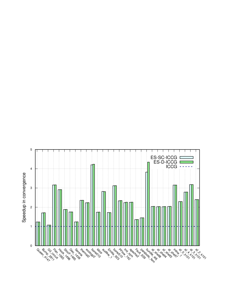
Figure 1: Speedup in convergence of ES-SC-ICCG and ES-D-ICCG over ICCG ($b$: random vector)

Table 2 lists the numerical results of the standard ICCG solver and its variants with the introduced convergence acceleration techniques, when a vector of ones is used for the right-hand side. ES-SC-ICCG denotes the CG solver with IC and subspace correction preconditioning based on the proposed error vector sampling method. ES-D-ICCG denotes the deflated ICCG solver using our technique. The table show the average computational time (sec) in 5 solution steps, which is denoted by $T_{t}$. Table 3 shows the results when random vectors are used for the right-hand side. The table shows the average number of iterations and computational time in 5 solution steps. The numerical results indicate that both solvers based on the proposed method achieve convergence acceleration for all 60 test cases (30 datasets $\times$ 2 kinds of right-hand side vectors). The convergence acceleration was significant for some of datasets. In the numerical tests using the vector of ones, the acceleration method attains more than 3-fold speedup in convergence for 16 out of 30 datasets. Even when we used random right-hand side vectors, the convergence was more than twice as fast as the ICCG solver for 20 out of 30 datasets as shown in Fig. 1.

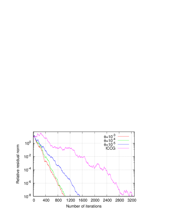
Figure 3: Convergence behavior of ES-D-ICCG (dataset: Flan_1565)

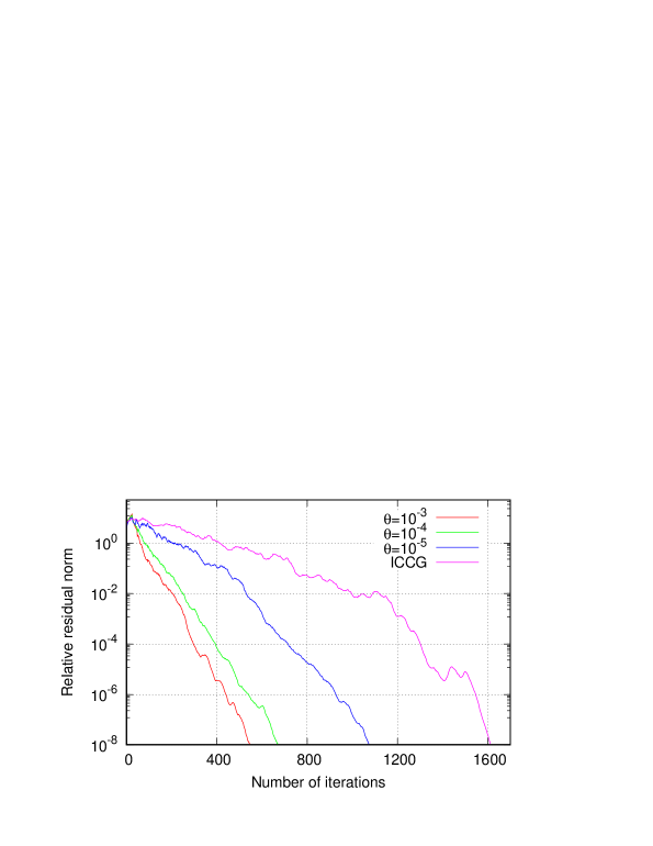
Figure 5: Convergence behavior of ES-D-ICCG (dataset: Hook_1498)

Figures 2, 3, 4, and 5 show the convergence behaviors of ES-SC-ICCG and ES-D-ICCG solvers for Flan_1565 and Hook_1498 datasets when a random vector is used for the right-hand side. The figures also confirm the effectiveness of the subspace correction and the deflation based on our technique. Numerical results imply that the larger $\theta$, which typically leads to larger $\tilde{m}$, results in the better convergence. This characteristic is also confirmed by the result listed in Tables 2 and 3. Figures 2, 3, 4, and 5 demonstrate that the convergence behaviors of two solvers are identical, though the treatments for the slow convergent error (eigenvectors associated with small eigenvalues) are different between two solvers ²⁹. While we examined the convergence behavior of the residual norm for all test cases, we observed that the convergence properties of two solvers were almost the same for most of test cases. The result indicates that the effects of the SC preconditioning and the deflation are similar when the coefficient matrix is diagonally scaled and the identical subspace that corresponds to eigenvectors associated with small eigenvalues is used.

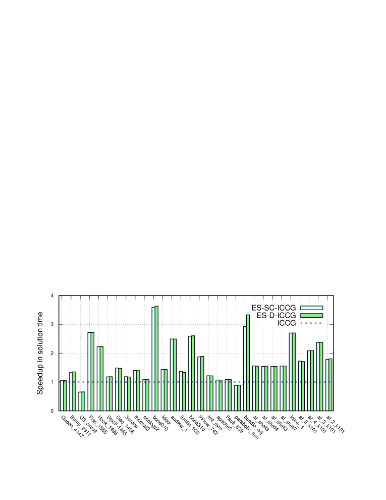
Figure 6: Speedup in computational time of ES-SC-ICCG and ES-D-ICCG over ICCG ($b$: random vector)

Next, we examine the computational time to solution. Table 2 shows that the solution time is reduced in 28 out of 30 cases in the tests using the right-hand side vector of ones. For 16 datasets, the computational time of the solvers using our technique (ES-SC- and ES-D-ICCG) is reduced to less than half of that of the normal ICCG solver. The performance difference between two solvers, ES-SC-ICCG and ES-D-ICCG is marginal. In the numerical test using random vectors, the computational time is also reduced in 28 out of 30 cases. Table 3 and Fig. 6 show the effectiveness of our technique in the random vector test. In these tests, performance improvement is not attained in the G3_circuit and parabolic_fem datasets, which have relatively small $nnz_{av}$ values. In (17), $\gamma_{sciccg}$ is enlarged when $nnz_{av}$ decreases. It means that it becomes difficult to obtain performance improvement in the solution time by the subspace correction preconditioning and the deflation method. In other words, for a dataset with a small $nnz_{av}$ value, the convergence rate should be substantially improved by the limited number of sample vectors to achieve solver performance improvement. In the numerical test, ES-SC-ICCG and ES-D-ICCG solvers obtained their best results for 12 out of 30 datasets when $\tilde{m}$ is equal to $m$ ($=$20). For these datasets, an increase in the number of sample vectors, $m$, possibly improves the solver performance.

5.2.2 Verification of the model for computational time per iteration

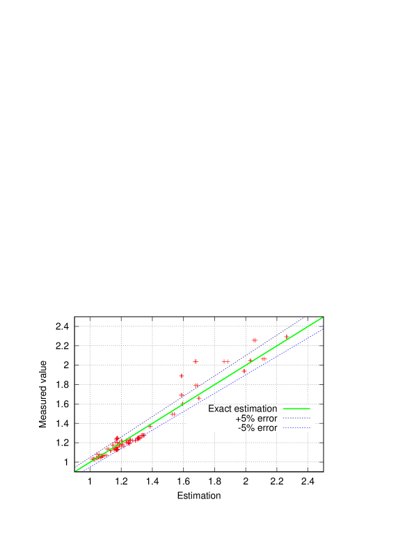
Figure 7: Comparison of estimated and measured values of computational time per iteration

The application of subspace correction or deflation typically leads to increase in the computational cost per iteration. In this subsection, we examine the performance model for iteration cost introduced in Sec. 4.4. In Fig. 7, we plot the measured and estimated values for the ratio of computational time of an ICCG iteration to that of an ES-SC- or ES-D-ICCG iteration. The estimated value for two solvers are given by (17). Figure 7 shows the result for all test cases, though only one mark is plotted for an identical $\tilde{m}$. For most of test cases, equation (17) gives good estimation for the ratio, and the error of the estimation is within $\pm$5%. Consequently, (17) can be used for estimation of the additional cost for subspace correction or deflation. However, in some test cases, especially when the measured value is over 2.0, relatively large estimation error is observed. These results arise in the G3_circuit, ecology2, and apache2 datasets. The coefficient matrices of these datasets commonly have a small number of nonzero elements per row ($nnz_{av}$) and a relatively structured nonzero element pattern. Namely, these matrices are derived from relatively simple problems, and (15) tends to give an overestimation for such a problem. Moreover, (17) implies that the impact of the additional cost for the convergence acceleration on the computational time tends to be large when $nnz_{av}$ is small. Accordingly, we recommend that the number of sampling vectors $m$ (the upper bound of $\tilde{m}$) should be small for a problem with small $nnz_{av}$.

5.2.3 Other factors on solver performance

Sampling method

In preliminary analyses, we compared two sampling methods A and B. Table 4 shows the results of the solver using the sampling method B for Flan_1565 and Hook_1498. In comparison of tables 2 and 4, the sampling method A gives better convergence acceleration than the method B. Because this tendency was observed for other test datasets, we decided to mainly use the sampling method A in our numerical tests. Moreover, the numerical test implies that the additional sampling of the approximation vector when the residual norm increases or stagnates is effective for improvement of the convergence acceleration effect. Because it is not straightforward to mathematically interpret the phenomenon, we intend to investigate the behavior of the error in the solution process in our future work based on numerical tests.

Sampling of residual vectors

In this paper, we consider the sampling of a relatively small number of vectors because it is practically important to save the additional memory space and computational cost. Considering other related techniques, the sampling of residual vectors might be of interest. We have an intuitive perspective for the comparison of sampling of error vectors and residual vectors. Because it holds that $A\mbox{\boldmath$e$}_{s}=\mbox{\boldmath$r$}_{s}$, the component corresponding small eigenvalues in $\mbox{\boldmath$e$}_{s}$ is numerically reduced in $\mbox{\boldmath$r$}_{s}$ by multiplication of $A$, where $\mbox{\boldmath$e$}_{s}$ and $\mbox{\boldmath$r$}_{s}$ are the sampled error and residual vectors, respectively. Consequently, it is expected that the error vector sampling is superior to the residual vector sampling to capture (approximate) eigenvectors that corresponds to small eigenvalues, which leads to better preconditioning effect for convergence. To verify our perspective, we conducted additional numerical tests of the solver using the residual vector sampling. In the numerical test using Flan_1565 and Hook_1498, it is shown that a small Ritz value less than $10^{-1}$ cannot be obtained and the convergence acceleration of the subspace correction and the deflation does not work well. Considering the numerical results, we can say that the error vector sampling outperforms the residual vector sampling to construct an effective mapping operator for subspaces used in the convergence acceleration techniques.

Verification of Ritz vector

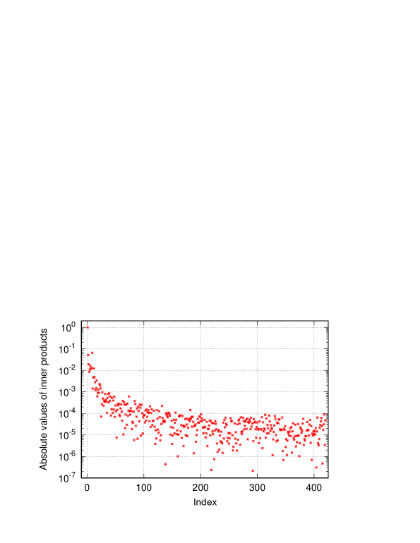
Figure 9: The absolute values of inner products, $\|(\tilde{\mbox{\boldmath$v$}}_{1},\mbox{\boldmath$v$}_{ir})\|,(ir=1,\ldots,420)$

In this section, we try to examine the property of Ritz vector calculated in our technique using a small size dataset (bccstk06: a 420 $\times$ 420 matrix). Figure 8 plots the eigenvalue distribution of the coefficient matrix and the Ritz values obtained in our method applied to a non-preconditioned CG solver. It is confirmed that some small eigenvalues including the smallest eigenvalue are well approximated by the obtained Ritz values. Moreover, we checked the orthogonality of the normalized Ritz vector that corresponds to the smallest Ritz value, $\tilde{\mbox{\boldmath$v$}}_{1}$, to the normalized eigenvectors of $A$ denoted by $\mbox{\boldmath$v$}_{ir},(ir=1,\ldots,420)$. It is noted that $ir$ is the index of eigenvalues in ascending order. Figure 9 shows the absolute value of the inner product $(\mbox{\boldmath$v$}_{r},\mbox{\boldmath$v$}_{ir})$. The magnitude of $|(\tilde{\mbox{\boldmath$v$}}_{1},\mbox{\boldmath$v$}_{1})|$ is close to 1 and it is substantially larger than those for other inner products, most of which are less than $10^{-3}$.

Table 2: Numerical results (sequential solver, $\mbox{\boldmath$b$}=(1,1,\ldots,1)^{\top}$)

		Queen_4147			Bump_2911			G3_circuit			Flan_1565			Hook_1498
Solver	$\theta$	$\tilde{m}$	#Ite.	$T_{t}$	$\tilde{m}$	#Ite.	$T_{t}$	$\tilde{m}$	#Ite.	$T_{t}$	$\tilde{m}$	#Ite.	$T_{t}$	$\tilde{m}$	#Ite.	$T_{t}$
ICCG		-	3128	2763	-	1551	584	-	898	44.8	-	3124	996	-	1617	287
ES-SC-ICCG	$10^{-3}$	20	995	1039	20	526	249	18	705	70.1	20	1082	398	20	472	108
	$10^{-4}$	19	2041	2121	18	824	382	9	707	54.8	19	1212	449	13	676	144
	$10^{-5}$	7	2816	2667	5	1118	445	1	887	49.6	8	1766	596	5	1080	209
ES-D-ICCG	$10^{-3}$	20	993	1036	20	459	218	18	702	70.1	20	942	347	20	469	108
	$10^{-4}$	19	2044	2120	18	821	381	9	706	54.1	19	1213	443	13	675	144
	$10^{-5}$	7	2818	2670	5	1117	449	1	887	49.8	8	1762	595	5	1078	209

		StocF-1465			Geo_1438			Serena			thermal2			ecology2
Solver	$\theta$	$\tilde{m}$	#Ite.	$T_{t}$	$\tilde{m}$	#Ite.	$T_{t}$	$\tilde{m}$	#Ite.	$T_{t}$	$\tilde{m}$	#Ite.	$T_{t}$	$\tilde{m}$	#Ite.	$T_{t}$
ICCG		-	56109	4741	-	443	79.6	-	301	55.7	-	2281	141	-	1823	49.7
ES-SC-ICCG	$10^{-3}$	20	14780	2011	15	248	58.2	7	243	49.6	20	849	89	20	813	50.1
	$10^{-4}$	20	14775	2001	2	387	72.5	0	-	-	17	994	99	15	902	48.5
	$10^{-5}$	20	14775	1998	0	-	-	0	-	-	4	1523	111	5	1329	50.3
ES-D-ICCG	$10^{-3}$	20	14731	1992	15	248	55.9	7	242	49.5	20	847	89	20	808	49.9
	$10^{-4}$	20	14717	1988	2	386	72.9	0	-	-	17	992	99	15	899	48.3
	$10^{-5}$	20	14717	2001	0	-	-	0	-	-	4	1519	111	5	1328	49.7

		bone010			ldoor			audikw_1			Emilia_923			boneS10
Solver	$\theta$	$\tilde{m}$	#Ite.	$T_{t}$	$\tilde{m}$	#Ite.	$T_{t}$	$\tilde{m}$	#Ite.	$T_{t}$	$\tilde{m}$	#Ite.	$T_{t}$	$\tilde{m}$	#Ite.	$T_{t}$
ICCG		-	4162	801	-	2160	293	-	2629	583	-	462	53.6	-	8532	1275
ES-SC-ICCG	$10^{-3}$	20	943	213	20	658	111	20	745	185	20	218	32.2	20	2688	486
	$10^{-4}$	18	967	216	16	1073	174	9	1138	265	19	266	38.9	20	2688	487
	$10^{-5}$	13	1302	280	3	1663	238	4	1521	343	5	373	46.5	20	2688	488
ES-D-ICCG	$10^{-3}$	20	935	211	20	655	110	20	756	188	20	201	29.7	20	2682	485
	$10^{-4}$	18	962	215	16	1072	173	9	1084	253	19	265	38.9	20	2682	485
	$10^{-5}$	13	1293	278	3	1662	237	4	1586	358	5	374	46.8	20	2682	486

		PFlow_742			tmt_sym			apache2			Fault_639			parabolic_fem
Solver	$\theta$	$\tilde{m}$	#Ite.	$T_{t}$	$\tilde{m}$	#Ite.	$T_{t}$	$\tilde{m}$	#Ite.	$T_{t}$	$\tilde{m}$	#Ite.	$T_{t}$	$\tilde{m}$	#Ite.	$T_{t}$
ICCG		-	33076	3357	-	1252	35.9	-	768	16.5	-	2187	177	-	1131	18.9
ES-SC-ICCG	$10^{-3}$	20	10359	1299	20	507	27.0	19	359	16.0	20	806	83	18	671	22.4
	$10^{-4}$	20	10360	1299	15	613	29.3	12	429	15.7	15	1366	134	7	862	20.7
	$10^{-5}$	20	10359	1299	3	1013	34.7	2	663	17.1	4	1905	164	0	-	-
ES-D-ICCG	$10^{-3}$	20	10269	1287	20	501	26.5	19	360	16.3	20	798	82	18	670	22.3
	$10^{-4}$	20	10269	1287	15	610	29.1	12	428	15.8	15	1364	133	7	861	20.7
	$10^{-5}$	20	10269	1285	3	1011	33.9	2	662	16.8	4	1901	164	0	-	-

		bundle_adj			af_shell8			af_shell4			af_shell3			af_shell7
Solver	$\theta$	$\tilde{m}$	#Ite.	$T_{t}$	$\tilde{m}$	#Ite.	$T_{t}$	$\tilde{m}$	#Ite.	$T_{t}$	$\tilde{m}$	#Ite.	$T_{t}$	$\tilde{m}$	#Ite.	$T_{t}$
ICCG		-	42809	2275	-	1048	52.0	-	1048	52.0	-	1048	52.3	-	1048	53.0
ES-SC-ICCG	$10^{-3}$	20	11705	824	18	483	31.4	18	481	31.1	18	481	31.4	18	483	31.5
	$10^{-4}$	18	11533	793	9	614	35.8	9	615	35.3	9	615	35.7	9	614	35.5
	$10^{-5}$	17	11460	781	0	-	-	0	-	-	0	-	-	0	-	-
ES-D-ICCG	$10^{-3}$	20	9740	686	18	481	31.4	18	479	31.0	18	479	31.4	18	481	31.5
	$10^{-4}$	18	10117	698	9	613	35.4	9	615	35.5	9	615	35.7	9	613	35.6
	$10^{-5}$	17	10532	717	0	-	-	0	-	-	0	-	-	0	-	-

		inline_1			af_0_k101			af_4_k101			af_3_k101			af_2_k101
Solver	$\theta$	$\tilde{m}$	#Ite.	$T_{t}$	$\tilde{m}$	#Ite.	$T_{t}$	$\tilde{m}$	#Ite.	$T_{t}$	$\tilde{m}$	#Ite.	$T_{t}$	$\tilde{m}$	#Ite.	$T_{t}$
ICCG		-	8487	879	-	12953	636	-	9993	489	-	8519	423	-	13092	648
ES-SC-ICCG	$10^{-3}$	20	2573	311	20	4153	276	20	3093	204	20	2632	176	20	4194	279
	$10^{-4}$	20	2572	310	20	4153	276	20	3094	204	20	2633	176	20	4194	279
	$10^{-5}$	19	2573	309	20	4153	275	20	3094	204	20	2632	176	20	4194	278
ES-D-ICCG	$10^{-3}$	20	2570	311	20	4150	275	20	3085	203	20	2624	175	20	4189	279
	$10^{-4}$	20	2571	311	20	4150	276	20	3086	203	20	2629	175	20	4189	278
	$10^{-5}$	19	2571	309	20	4150	275	20	3086	204	20	2624	175	20	4189	279

Table 3: Numerical results (sequential solver, $b$: random vector)

		Queen_4147			Bump_2911			G3_circuit			Flan_1565			Hook_1498
Solver	$\theta$	$\tilde{m}$	#Ite.	$T_{t}$	$\tilde{m}$	#Ite.	$T_{t}$	$\tilde{m}$	#Ite.	$T_{t}$	$\tilde{m}$	#Ite.	$T_{t}$	$\tilde{m}$	#Ite.	$T_{t}$
ICCG	-	-	3140	2776	-	1544	564	-	926	46.1	-	3196	1010	-	1613	282
ES-SC-ICCG	$10^{-3}$	20	2546	2648	20	906	428	19	865	88.8	20	1013	372	20	554	127
	$10^{-4}$	19	2566	2652	17	921	422	10	891	70.6	19	1048	382	13	672	143
	$10^{-5}$	7	2783	2626	5	1114	441	0	-	-	9	1524	518	5	1076	208
ES-D-ICCG	$10^{-3}$	20	2542	2652	20	900	424	19	863	88.2	20	1011	372	20	553	126
	$10^{-4}$	19	2561	2654	17	917	418	10	890	70.2	19	1048	383	13	671	141
	$10^{-5}$	7	2779	2630	5	1113	439	0	-	-	9	1523	517	5	1075	206

		StocF-1465			Geo_1438			Serena			thermal2			ecology2
Solver	$\theta$	$\tilde{m}$	#Ite.	$T_{t}$	$\tilde{m}$	#Ite.	$T_{t}$	$\tilde{m}$	#Ite.	$T_{t}$	$\tilde{m}$	#Ite.	$T_{t}$	$\tilde{m}$	#Ite.	$T_{t}$
ICCG		-	55799	4714	-	441	81.3	-	299	58.1	-	2261	141	-	1902	51.7
ES-SC-ICCG	$10^{-3}$	20	29693	4001	15	252	54.7	7	242	49.1	20	959	101	20	853	52.5
	$10^{-4}$	20	29693	4011	2	385	71.9	0	-	-	17	1020	101	16	933	51.5
	$10^{-5}$	20	29693	4007	0	-	-	0	-	-	4	1526	112	5	1268	47.8
ES-D-ICCG	$10^{-3}$	20	29600	3990	15	251	55.1	7	241	49.6	20	957	100	20	850	52.2
	$10^{-4}$	20	29600	3993	2	384	72.3	0	-	-	17	1019	101	16	930	51.2
	$10^{-5}$	20	29600	4002	0	-	-	0	-	-	4	1524	111	5	1267	47.4

		bone010			ldoor			audikw_1			Emilia_923			boneS10
Solver	$\theta$	$\tilde{m}$	#Ite.	$T_{t}$	$\tilde{m}$	#Ite.	$T_{t}$	$\tilde{m}$	#Ite.	$T_{t}$	$\tilde{m}$	#Ite.	$T_{t}$	$\tilde{m}$	#Ite.	$T_{t}$
ICCG		-	4189	804	-	2143	293	-	2420	533	-	459	54	-	8515	1274
ES-SC-ICCG	$10^{-3}$	20	996	225	20	1230	208	19	858	214	20	266	39	20	2733	492
	$10^{-4}$	17	1060	234	16	1259	204	8	1220	284	18	276	40	20	2733	494
	$10^{-5}$	13	1288	277	3	1649	236	4	1604	364	5	371	46	20	2733	494
ES-D-ICCG	$10^{-3}$	20	989	221	20	1227	206	19	861	214	20	267	40	20	2728	490
	$10^{-4}$	17	1053	231	16	1256	203	8	1207	280	18	276	40	20	2728	490
	$10^{-5}$	13	1281	273	3	1648	234	4	1579	356	5	370	47	20	2728	490

		PFlow_742			tmt_sym			apache2			Fault_639			parabolic_fem
Solver	$\theta$	$\tilde{m}$	#Ite.	$T_{t}$	$\tilde{m}$	#Ite.	$T_{t}$	$\tilde{m}$	#Ite.	$T_{t}$	$\tilde{m}$	#Ite.	$T_{t}$	$\tilde{m}$	#Ite.	$T_{t}$
ICCG		-	32971	3311	-	1256	35.8	-	770	16.8	-	2172	176	-	1208	20.1
ES-SC-ICCG	$10^{-3}$	20	14148	1774	20	562	29.8	20	342	15.7	20	1601	162	18	835	27.6
	$10^{-4}$	20	14148	1772	15	617	29.5	12	445	16.4	16	1629	159	9	889	22.8
	$10^{-5}$	20	14148	1769	3	1002	33.9	2	653	16.7	4	1899	162	0	-	-
ES-D-ICCG	$10^{-3}$	20	14042	1758	20	556	29.8	20	341	15.7	20	1595	163	18	833	27.6
	$10^{-4}$	20	14042	1758	15	614	29.5	12	444	16.4	16	1623	159	9	888	22.6
	$10^{-5}$	20	14042	1754	3	1000	33.8	2	653	16.6	4	1896	162	0	-	-

		bundle_adj			af_shell8			af_shell4			af_shell3			af_shell7
Solver	$\theta$	$\tilde{m}$	#Ite.	$T_{t}$	$\tilde{m}$	#Ite.	$T_{t}$	$\tilde{m}$	#Ite.	$T_{t}$	$\tilde{m}$	#Ite.	$T_{t}$	$\tilde{m}$	#Ite.	$T_{t}$
ICCG		-	43578	2325	-	1038	51.2	-	1039	51.7	-	1039	51.1	-	1038	51.6
ES-SC-ICCG	$10^{-3}$	20	11997	846	18	510	32.8	18	513	33.5	18	513	33.2	18	510	33.2
	$10^{-4}$	19	11394	795	9	606	34.9	9	602	34.9	9	602	34.7	9	606	35.2
	$10^{-5}$	19	11394	795	0	-	-	0	-	-	0	-	-	0	-	-
ES-D-ICCG	$10^{-3}$	20	10110	711	18	508	33.0	18	511	33.4	18	511	33.1	18	508	33.1
	$10^{-4}$	19	10030	700	9	605	34.9	9	601	34.9	9	601	34.7	9	605	35.1
	$10^{-5}$	19	10030	698	0	-	-	0	-	-	0	-	-	0	-	-

		inline_1			af_0_k101			af_4_k101			af_3_k101			af_2_k101
Solver	$\theta$	$\tilde{m}$	#Ite.	$T_{t}$	$\tilde{m}$	#Ite.	$T_{t}$	$\tilde{m}$	#Ite.	$T_{t}$	$\tilde{m}$	#Ite.	$T_{t}$	$\tilde{m}$	#Ite.	$T_{t}$
ICCG		-	8464	870	-	12961	641	-	9974	495	-	8501	420	-	12970	641
ES-SC-ICCG	$10^{-3}$	20	2686	324	20	5657	372	20	3582	238	20	2680	177	20	5413	361
	$10^{-4}$	20	2686	324	20	5657	372	20	3582	238	20	2680	177	20	5413	360
	$10^{-5}$	19	2686	322	20	5657	372	20	3582	238	20	2680	177	20	5413	360
ES-D-ICCG	$10^{-3}$	20	2683	324	20	5649	376	20	3575	238	20	2676	177	20	5409	356
	$10^{-4}$	20	2683	324	20	5649	376	20	3575	238	20	2676	177	20	5409	356
	$10^{-5}$	19	2684	322	20	5649	376	20	3575	237	20	2676	177	20	5409	355

Figure 2: Convergence behavior of ES-SC-ICCG (dataset: Flan_1565)

Figure 4: Convergence behavior of ES-SC-ICCG (dataset: Hook_1498)

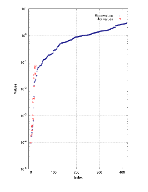
Figure 8: Comparison of eigenvalues and Ritz values (dataset: bcsstik06, $n$=420, $m$=20)

5.3 Numerical results on the parallel solver

In this subsection, we report the results of parallel (multithreaded) solver. The parallelization of the CG solver is relatively straightforward. But, the IC preconditioning step that consists of forward and backward substitutions is not naturally parallelized. While there are various parallel processing methods, we use one of simple but popular methods, namely block Jacobi IC preconditioning ³⁰ in the present research. The parallelization of the subspace correction preconditioning and the deflation method is relatively easy. The computationally dominant part for these methods is dense matrix vector multiplication, which can be straightforwardly parallelized. Because $\tilde{m}$ is typically tiny, we sequentially process the solution part for the linear system with an $\tilde{m}\times\tilde{m}$ coefficient matrix $W^{\top}AW$ that is involved in the methods.

Tables 5 and 6 list the numerical results of the parallel ICCG solver and its variants with the proposed techniques, when a vector of ones and random vectors are used, respectively. From the viewpoint of convergence, the results on the parallel solver are similar to those of the sequential solver. For all 60 test cases (30 datasets $\times$ 2 kinds of right-hand side vectors), convergence acceleration was attained by the proposed method. When a vector of ones was used, the convergence was more than twice as fast as the parallel ICCG solver for 27 out of 30 datasets. Figure 10 shows the speedup in the convergence of the parallel solver based on the proposed technique against the parallel ICCG solver, when random vectors are used for the right-hand side vectors. In the test using random vectors, the proposed method attains more than 2-fold speedup in convergence compared to the parallel ICCG solver for 21 out of 30 datasets.

Next, we examine the computational time. In the test using a vector of ones, the proposed method reduces the solution time for 28 out of 30 datasets. For the bundle_adj dataset, the parallel deflated ICCG solver based on our technique attains more than 4-fold speedup compared to the parallel ICCG solver. The test using random vectors also indicates that our technique is effective to reduce the computational time for most of test datasets (25 out of 30). In block Jacobi IC preconditioning, the computational cost for a PCG iteration is reduced as the number of threads increases. Consequently, the impact of the additional cost for the convergence acceleration (subspace correction preconditioning or deflation) on the preconditioned solver is substantially enlarged in the parallel execution by many threads. In other words, the ratio of the iteration costs is enlarged from (17). Because we used a number of threads (= 40) in our numerical tests, it becomes difficult to reduce the solution time compared with the sequential solver. However, Fig. 11 indicates that our convergence acceleration technique accelerates the solution process for most of test problems.

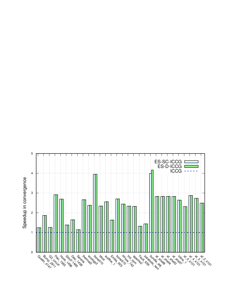
Figure 10: Speedup in convergence of ES-SC-ICCG and ES-D-ICCG over ICCG (Parallel multithreaded solver, $b$: random vector)

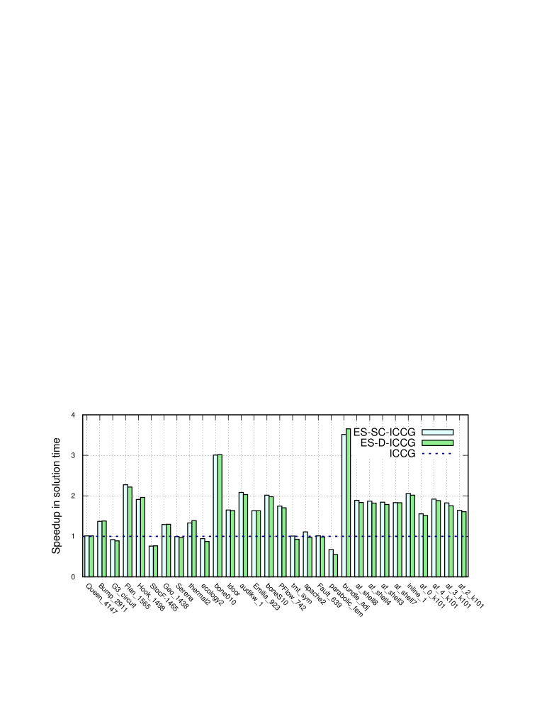
Figure 11: Speedup in computational time of ES-SC-ICCG and ES-D-ICCG over pICCG (Parallel multithreaded solver, $b$: random vector)

5.4 Condition number estimation

Figure 8 implies that our technique based on error vector sampling can be a useful tool for the estimation of the smallest eigenvalue. Because the estimation of the largest eigenvalue is relatively easy, the technique can be used for the estimation of the condition number of the coefficient matrix. Algorithm 2 shows the proposed procedure of PCG method with a condition number estimation. The largest eigenvalue is estimated by the power method which is combined with the procedure of CG method. The smallest eigenvalue is estimated by our technique. We conducted numerical tests using five relatively small matrices downloaded from SuiteSparse matrix collection to examine our technique. Diagonal scaling is applied to the matrices before the tests. Table 7 shows the estimation for the largest eigenvalue $\lambda_{max}$, the smallest eigenvalue $\lambda_{min}$, and the condition number $\kappa$ compared with the results calculated by the LAPACK library. Table 7 implies that the technique based on the error sampling is effective for the estimation of the condition number.

Because the number of sample vectors is much smaller than $n$ ($m\ll n$), the additional computational cost for the calculation of the smallest eigenvalue (Ritz value) is typically negligible compared with the iterative solution cost. Although the power method requires an additional sparse matrix vector multiplication (SpMV) operation, it is combined with the SpMV for CG method. In this case, the matrix data transferred from main memory are efficiently used for two vectors. Because the SpMV operation is typically memory bound, the impact of the power method on the iteration time is possibly limited. Most of iterative solvers like CG solver usually uses a convergence criterion based on a (relative) residual norm. If the estimation of the condition number of the coefficient matrix is given with the solution vector by the iterative solver, it can be a useful tool to evaluate the accuracy of the solution vector. The proposed solver provides this function without large amount of additional computations.

Algorithm 2 PCG method with condition number estimation

1:$A$, $b$, $M$, $\mbox{\boldmath$x$}_{0}$, $\varepsilon$, $m$

2:$\mbox{\boldmath$r$}_{0}=\mbox{\boldmath$b$}-A\mbox{\boldmath$x$}_{0}$

3:$\mbox{\boldmath$v$}_{0}\leftarrow$ Initialization (a unit random vector etc.)

4:for $i=1,2,\ldots$ do

5:     $\mbox{\boldmath$z$}_{i-1}=M^{-1}\mbox{\boldmath$r$}_{i-1}$

6:     $\rho_{i-1}=(\mbox{\boldmath$r$}_{i-1},\mbox{\boldmath$z$}_{i-1})$

7:     if i=1 then

8:         $\mbox{\boldmath$p$}_{1}=\mbox{\boldmath$z$}_{0}$

9:     else

10:         $\beta_{i-1}=\rho_{i-1}/\rho_{i-2}$

11:         $\mbox{\boldmath$p$}_{i}=\mbox{\boldmath$z$}_{i-1}+\beta_{i-1}\mbox{\boldmath$p$}_{i-1}$

12:     end if

13:     $(\mbox{\boldmath$q$}_{i}\ \mbox{\boldmath$v$}_{i})=A(\mbox{\boldmath$p$}_{i}\ \mbox{\boldmath$v$}_{i-1})$    // (SpMV)

14:     $\mbox{\boldmath$v$}_{i}=\mbox{\boldmath$v$}_{i}/\|\mbox{\boldmath$v$}_{i}\|_{2}$

15:     $\alpha_{i}=\rho_{i-1}/(\mbox{\boldmath$p$}_{i},\mbox{\boldmath$q$}_{i})$

16:     $\mbox{\boldmath$x$}_{i}=\mbox{\boldmath$x$}_{i-1}+\alpha_{i}\mbox{\boldmath$p$}_{i}$

17:     $\mbox{\boldmath$r$}_{i}=\mbox{\boldmath$r$}_{i-1}-\alpha_{i}\mbox{\boldmath$q$}_{i}$

18:     if $\|\mbox{\boldmath$r$}_{i}\|_{2}\leq\varepsilon\|\mbox{\boldmath$b$}\|_{2}$ then

19:         break

20:     end if

21:     if Sampling condition is satisfied then

22:         $\tilde{\mbox{\boldmath$x$}}^{(s)}=\mbox{\boldmath$x$}_{i},\ s\in\{1,2,\ldots,m\}$

23:     end if

24:end for

25:$\tilde{E}=(\mbox{\boldmath$x$}_{i}-\tilde{\mbox{\boldmath$x$}}^{(1)}\,\mbox{\boldmath$x$}_{i}-\tilde{\mbox{\boldmath$x$}}^{(2)}\,\ldots\,\mbox{\boldmath$x$}_{i}-\tilde{\mbox{\boldmath$x$}}^{(m)})$

26:Apply Gram-Schmidt method to $\tilde{E}$ and obtain $E$

27:Solve an eigenvalue problem: $E^{\top}AE\mbox{\boldmath$t$}=\lambda\mbox{\boldmath$t$}$ and obtain the smallest Ritz value $\lambda_{min}$

28:$\lambda_{max}=(\mbox{\boldmath$v$}_{i},A\mbox{\boldmath$v$}_{i})$

29:$\kappa=\lambda_{max}/\lambda_{min}$

30:$\mbox{\boldmath$x$}_{i}$, $\kappa$

6 Conclusion

In this paper, we introduce an algebraic auxiliary matrix construction method that can be used for the subspace correction preconditioning and the deflation method. We focus on a problem in which a sequence of linear systems with an identical coefficient matrix are solved. In our method, we sample the approximate solution vectors in the first iterative solution step, and calculate the error vectors corresponding to the sample vectors after the solution step is completed. Then, we perform the Rayleigh-Ritz method using a subspace spanned by these error vectors to identify (approximate) eigenvectors associated with small eigenvalues. Finally, the auxiliary matrix is constructed by the Ritz vectors associated with small Ritz values. We also present a cost model of the subspace preconditioning and the deflation method. Numerical tests using 30 coefficient matrices were conducted to verify our technique. The test results confirm that the proposed convergence acceleration technique efficiently reduces both the number of iterations for the convergence and the solution time of the serial and parallel preconditioned CG solvers. Moreover, additional numerical tests indicate that the proposed technique can be used for the condition number estimation.

Currently, we examine the effectiveness of the technique for a linear system having an unsymmetric coefficient matrix. Because the preliminary results show its effectiveness, we will report it in future. We are also investigating application of the technique to other problems. Especially, we examine the effectiveness in parallel-in-time (PinT) simulations, which often involves the solution process of multiple linear systems of coefficient matrices having a common property. We are also interested in the combination of our technique with preconditioning techniques suitable for GPU computing. In future, we will examine our technique in various situations of computational science or engineering problems.

Table 4: Solver performance using sampling method B (sequential solver, $\mbox{\boldmath$b$}=(1,1,\ldots,1)^{\top}$)

		Flan_1565			Hook_1498
Solver	$\theta$	$\tilde{m}$	#Ite.	$T_{t}$	$\tilde{m}$	#Ite.	$T_{t}$
ES-SC-ICCG	$10^{-3}$	20	1584	586	15	1075	233
	$10^{-4}$	15	1927	690	7	1157	229
	$10^{-5}$	7	2094	706	4	1208	230
ES-D-ICCG	$10^{-3}$	20	1579	585	15	1072	232
	$10^{-4}$	15	1925	687	7	1156	229
	$10^{-5}$	7	2093	704	5	1207	229

Table 5: Numerical results (parallel solver, $\mbox{\boldmath$b$}=(1,1,\ldots,1)^{\top}$)

		Queen_4147			Bump_2911			G3_circuit			Flan_1565			Hook_1498
Solver	$\theta$	$\tilde{m}$	#Ite.	$T_{t}$	$\tilde{m}$	#Ite.	$T_{t}$	$\tilde{m}$	#Ite.	$T_{t}$	$\tilde{m}$	#Ite.	$T_{t}$	$\tilde{m}$	#Ite.	$T_{t}$
ICCG		-	4663	215	-	3455	73.4	-	1461	5.40	-	4911	86.6	-	2312	23.4
ES-SC-ICCG	$10^{-3}$	20	1532	89	20	1062	30.8	20	468	3.81	20	1504	31.3	19.0	808	11.6
	$10^{-4}$	20	1532	88	17	1814	51.1	13	1067	7.22	18	1777	37.3	13.0	1036	13.9
	$10^{-5}$	6	4258	218	2	2977	68.1	2	1392	5.67	9	2415	47.2	5.0	1562	18.8
ES-D-ICCG	$10^{-3}$	20	1530	91	20	1062	31.3	20	468	3.90	20	1502	33.0	19.0	807	12.1
	$10^{-4}$	20	1530	93	17	1811	51.4	13	1066	7.08	18	1776	38.2	13.0	1035	14.3
	$10^{-5}$	6	4252	216	2	2977	68.7	2	1392	5.73	9	2409	46.6	5.0	1561	18.9

		StocF-1465			Geo_1438			Serena			thermal2			ecology2
Solver	$\theta$	$\tilde{m}$	#Ite.	$T_{t}$	$\tilde{m}$	#Ite.	$T_{t}$	$\tilde{m}$	#Ite.	$T_{t}$	$\tilde{m}$	#Ite.	$T_{t}$	$\tilde{m}$	#Ite.	$T_{t}$
ICCG		-	66348	329	-	904	9.62	-	628	6.77	-	3583	12.0	-	2131	3.29
ES-SC-ICCG	$10^{-3}$	20	16453	157	14	549	7.26	8	546	6.36	20	1128	8.1	20	885	4.40
	$10^{-4}$	20	16453	154	2	779	8.24	0	-	-	17	1555	10.7	15	1039	4.19
	$10^{-5}$	20	16453	157	0	-	-	0	-	-	4	2506	10.4	4	1656	3.95
ES-D-ICCG	$10^{-3}$	20	16452	148	14	548	7.27	8	545	6.39	20	1126	8.0	20	882	4.38
	$10^{-4}$	20	16452	147	2	778	8.40	0	-	-	17	1554	10.2	15	1037	4.33
	$10^{-5}$	20	16452	150	0	-	-	0	-	-	4	2504	10.8	4	1654	4.05

		bone010			ldoor			audikw_1			Emilia_923			boneS10
Solver	$\theta$	$\tilde{m}$	#Ite.	$T_{t}$	$\tilde{m}$	#Ite.	$T_{t}$	$\tilde{m}$	#Ite.	$T_{t}$	$\tilde{m}$	#Ite.	$T_{t}$	$\tilde{m}$	#Ite.	$T_{t}$
ICCG		-	7838	76.9	-	5227	38.0	-	2635	30.0	-	6542	42.1	-	14690	119
ES-SC-ICCG	$10^{-3}$	20	2141	29.6	20	1503	14.8	20	816	11.4	20	1893	17.3	20	5166	55
	$10^{-4}$	18	2207	28.6	18	2199	20.7	7	1549	19.1	19	2991	27.5	20	5164	56
	$10^{-5}$	12	2925	35.7	3	4040	29.6	3	1798	21.2	7	4829	36.0	19	5446	58
ES-D-ICCG	$10^{-3}$	20	2138	28.9	20	1504	14.8	20	813	11.6	20	1895	17.8	20	5162	57
	$10^{-4}$	18	2203	28.9	18	2196	20.9	7	1545	19.3	19	2989	29.1	20	5161	56
	$10^{-5}$	12	2921	36.3	3	4036	30.8	3	1796	21.9	7	4823	37.1	19	5446	59

		PFlow_742			tmt_sym			apache2			Fault_639			parabolic_fem
Solver	$\theta$	$\tilde{m}$	#Ite.	$T_{t}$	$\tilde{m}$	#Ite.	$T_{t}$	$\tilde{m}$	#Ite.	$T_{t}$	$\tilde{m}$	#Ite.	$T_{t}$	$\tilde{m}$	#Ite.	$T_{t}$
ICCG		-	37485	214	-	1576	2.26	-	1056	1.31	-	5083	26.2	-	2125	1.58
ES-SC-ICCG	$10^{-3}$	20	11633	95	20	638	2.40	19	408	1.51	20	1496	9.6	19	1419	3.50
	$10^{-4}$	20	11633	95	14	777	2.33	12	494	1.27	18	3075	19.4	8	1326	1.89
	$10^{-5}$	20	11633	99	3	1259	2.09	3	816	1.31	2	4735	22.6	0	-	-
ES-D-ICCG	$10^{-3}$	20	11617	100	20	636	2.44	19	408	1.53	20	1495	9.6	19	1417	4.03
	$10^{-4}$	20	11617	97	14	776	2.35	12	494	1.39	18	3074	18.8	8	1325	2.27
	$10^{-5}$	20	11617	102	3	1257	2.30	3	815	1.43	2	4739	22.2	0	-	-

		bundle_adj			af_shell8			af_shell4			af_shell3			af_shell7
Solver	$\theta$	$\tilde{m}$	#Ite.	$T_{t}$	$\tilde{m}$	#Ite.	$T_{t}$	$\tilde{m}$	#Ite.	$T_{t}$	$\tilde{m}$	#Ite.	$T_{t}$	$\tilde{m}$	#Ite.	$T_{t}$
ICCG		-	64356	797	-	1575	5.13	-	1575	5.31	-	1575	5.07	-	1575	4.91
ES-SC-ICCG	$10^{-3}$	20	14407	208	20	537	2.58	20	539	2.59	20	539	2.62	20	537	2.56
	$10^{-4}$	20	14407	207	11	764	3.08	11	764	3.10	11	764	3.17	11	764	3.07
	$10^{-5}$	19	14104	200	0	-	-	0	-	-	0	-	-	0	-	-
ES-D-ICCG	$10^{-3}$	20	13547	196	20	537	2.64	20	537	2.76	20	537	2.65	20	537	2.59
	$10^{-4}$	20	13547	196	11	764	3.25	11	763	3.33	11	763	3.24	11	764	3.20
	$10^{-5}$	19	13611	194	0	-	-	0	-	-	0	-	-	0	-	-

		inline_1			af_0_k101			af_4_k101			af_3_k101			af_2_k101
Solver	$\theta$	$\tilde{m}$	#Ite.	$T_{t}$	$\tilde{m}$	#Ite.	$T_{t}$	$\tilde{m}$	#Ite.	$T_{t}$	$\tilde{m}$	#Ite.	$T_{t}$	$\tilde{m}$	#Ite.	$T_{t}$
ICCG		-	23064	115	-	16157	48.6	-	12458	45.5	-	10595	34.9	-	16249	57.6
ES-SC-ICCG	$10^{-3}$	20	6393	44	20	5026	24.7	20	4230	20.7	20	3567	17.1	20	4924	24.6
	$10^{-4}$	20	6393	43	20	5026	23.9	20	4230	19.7	20	3567	16.9	20	4924	23.7
	$10^{-5}$	18	8969	60	20	5026	24.1	20	4230	19.5	20	3567	16.8	20	4924	22.8
ES-D-ICCG	$10^{-3}$	20	6390	46	20	5018	24.8	20	4237	21.6	20	3574	18.0	20	4920	24.9
	$10^{-4}$	20	6390	46	20	5018	24.7	20	4237	20.8	20	3574	17.6	20	4920	24.5
	$10^{-5}$	18	8964	62	20	5018	25.2	20	4237	20.4	20	3574	17.5	20	4920	24.4

Table 6: Numerical results (parallel solver, $b$: random vector)

		Queen_4147			Bump_2911			G3_circuit			Flan_1565			Hook_1498
Solver	$\theta$	$\tilde{m}$	#Ite.	$T_{t}$	$\tilde{m}$	#Ite.	$T_{t}$	$\tilde{m}$	#Ite.	$T_{t}$	$\tilde{m}$	#Ite.	$T_{t}$	$\tilde{m}$	#Ite.	$T_{t}$
ICCG		-	4684	215	-	3437	73.9	-	1455	5.27	-	4906	83.6	-	2309	24.3
ES-SC-ICCG	$10^{-3}$	20	3762	217	20	1844	53.9	20	1157	9.54	20	1684	36.8	19.0	858	12.7
	$10^{-4}$	19	3760	217	17	1929	54.6	13	1203	8.15	18	1768	37.8	13.0	1027	13.6
	$10^{-5}$	6	4166	212	2	2967	67.8	2	1388	5.74	9	2411	47.3	5.0	1557	18.3
ES-D-ICCG	$10^{-3}$	20	3761	220	20	1842	53.5	20	1159	9.71	20	1684	37.7	19	857	12.4
	$10^{-4}$	19	3758	218	17	1927	53.8	13	1202	8.24	18	1766	38.5	13	1026	13.9
	$10^{-5}$	6	4164	212	2	2964	67.0	2	1388	5.94	9	2410	48.2	5.0	1556	18.6

		StocF-1465			Geo_1438			Serena			thermal2			ecology2
Solver	$\theta$	$\tilde{m}$	#Ite.	$T_{t}$	$\tilde{m}$	#Ite.	$T_{t}$	$\tilde{m}$	#Ite.	$T_{t}$	$\tilde{m}$	#Ite.	$T_{t}$	$\tilde{m}$	#Ite.	$T_{t}$
ICCG		-	51167	258	-	901	9.37	20	625	6.49	-	3569	12.5	-	2225	3.48
ES-SC-ICCG	$10^{-3}$	20	37038	341	14	548	7.26	8	546	6.53	20	1343	9.4	20	937	4.67
	$10^{-4}$	20	37038	341	2	774	8.49	0	-	-	17	1597	10.4	17	1045	4.74
	$10^{-5}$	20	37038	342	0	-	-	0	-	-	4	2466	10.6	5	1471	3.69
ES-D-ICCG	$10^{-3}$	20	37036	342	14	547	7.22	8	545	6.69	20	1342	9.1	20	935	4.55
	$10^{-4}$	20	37036	340	2	773	8.57	0	-	-	17	1596	10.2	17	1044	4.64
	$10^{-5}$	20	37036	337	0	-	-	0	-	-	4	2465	10.8	5	1469	3.99

		bone010			ldoor			audikw_1			Emilia_923			boneS10
Solver	$\theta$	$\tilde{m}$	#Ite.	$T_{t}$	$\tilde{m}$	#Ite.	$T_{t}$	$\tilde{m}$	#Ite.	$T_{t}$	$\tilde{m}$	#Ite.	$T_{t}$	$\tilde{m}$	#Ite.	$T_{t}$
ICCG			8190	84.1	-	5198	36.2	-	2633	30.2	-	6507	43.0	-	14637	119
ES-SC-ICCG	$10^{-3}$	20	2077	28.3	20	2222	22.0	20	1031	14.5	20	3989	35.4	20	5422	60
	$10^{-4}$	19	2100	28.0	18	2320	21.9	7	1541	19.4	19	4027	36.7	20	5422	59
	$10^{-5}$	12	2883	35.6	3	4019	30.1	3	1791	21.7	7	4798	36.8	19	5432	59
ES-D-ICCG	$10^{-3}$	20	2074	27.9	20	2220	22.6	20	1028	14.9	20	3986	37.7	20	5419	61
	$10^{-4}$	19	2096	28.4	18	2319	22.1	7	1536	19.9	19	4026	37.9	20	5419	62
	$10^{-5}$	12	2870	37.1	3	4016	31.2	3	1789	21.8	7	4797	36.9	19	5428	60

		PFlow_742			tmt_sym			apache2			Fault_639			parabolic_fem
Solver	$\theta$	$\tilde{m}$	#Ite.	$T_{t}$	$\tilde{m}$	#Ite.	$T_{t}$	$\tilde{m}$	#Ite.	$T_{t}$	$\tilde{m}$	#Ite.	$T_{t}$	$\tilde{m}$	#Ite.	$T_{t}$
ICCG		-	37486	221	-	1569	2.13	-	1055	1.34	-	5047	22.7	-	2583	1.89
ES-SC-ICCG	$10^{-3}$	20	15380	127	20	673	2.53	19	454	1.68	20	3828	24.9	19	1798	4.33
	$10^{-4}$	20	15380	127	14	784	2.51	12	499	1.37	18	3872	24.3	9	1885	2.80
	$10^{-5}$	20	15380	130	3	1256	2.12	3	810	1.21	2	4710	22.4	0	-	-
ES-D-ICCG	$10^{-3}$	20	15354	131	20	671	2.55	19	454	1.64	20	3830	24.9	19	1797	4.84
	$10^{-4}$	20	15354	130	14	782	2.53	12	498	1.51	18	3869	24.6	9	1885	3.42
	$10^{-5}$	20	15354	133	3	1255	2.30	3	809	1.38	2	4708	23.0	0	-	-

		bundle_adj			af_shell8			af_shell4			af_shell3			af_shell7
Solver	$\theta$	$\tilde{m}$	#Ite.	$T_{t}$	$\tilde{m}$	#Ite.	$T_{t}$	$\tilde{m}$	#Ite.	$T_{t}$	$\tilde{m}$	#Ite.	$T_{t}$	$\tilde{m}$	#Ite.	$T_{t}$
ICCG		-	55336	701	-	1572	5.07	-	1572	5.06	-	1572	4.95	-	1572	5.04
ES-SC-ICCG	$10^{-3}$	20	13873	199	20	557	2.69	20	556	2.71	20	556	2.68	20	557	2.75
	$10^{-4}$	20	13873	200	11	760	3.05	11	760	3.04	11	760	3.04	11	760	3.03
	$10^{-5}$	19	13947	200	0	-	-	0	-	-	0	-	-	0	-	-
ES-D-ICCG	$10^{-3}$	20	13287	192	20	555	2.76	20	555	2.78	20	555	2.77	20	555	2.75
	$10^{-4}$	20	13287	193	11	759	3.23	11	759	3.21	11	759	3.19	11	759	3.22
	$10^{-5}$	19	13796	199	0	-	-	0	-	-	0	-	-	0	-	-

		inline_1			af_0_k101			af_4_k101			af_3_k101			af_2_k101
Solver	$\theta$	$\tilde{m}$	#Ite.	$T_{t}$	$\tilde{m}$	#Ite.	$T_{t}$	$\tilde{m}$	#Ite.	$T_{t}$	$\tilde{m}$	#Ite.	$T_{t}$	$\tilde{m}$	#Ite.	$T_{t}$
ICCG		-	23054	124	-	16121	51.5	-	12425	39.9	-	10584	33.7	-	16237	50.9
ES-SC-ICCG	$10^{-3}$	20	8738	60	20	6977	33.1	20	4327	20.8	20	3877	19.6	20	6526	31.0
	$10^{-4}$	20	8738	61	20	6977	33.1	20	4327	20.9	20	3877	18.8	20	6526	31.1
	$10^{-5}$	18	9090	62	20	6977	33.5	20	4327	20.5	20	3877	18.5	20	6526	31.3
ES-D-ICCG	$10^{-3}$	20	8732	61	20	6966	34.0	20	4322	21.2	20	3873	19.2	20	6523	32.1
	$10^{-4}$	20	8732	62	20	6966	34.6	20	4322	21.2	20	3873	19.3	20	6523	31.7
	$10^{-5}$	18	9086	65	20	6966	34.5	20	4322	21.3	20	3873	19.3	20	6523	32.2

Table 7: Condition number estimation based on error vector sampling

	Estimation			LAPACK
Dataset	$\lambda_{max}$	$\lambda_{min}$	$\kappa$	$\lambda_{max}$	$\lambda_{min}$	$\kappa$
bcsstk07	2.88	9.11$\times 10^{-5}$	3.16$\times 10^{4}$	2.90	9.11$\times 10^{-5}$	3.18$\times 10^{4}$
msc01440	3.62	3.08$\times 10^{-4}$	1.18$\times 10^{4}$	3.62	2.86$\times 10^{-4}$	1.27$\times 10^{4}$
ex33	3.93	2.86$\times 10^{-11}$	1.37$\times 10^{11}$	3.93	2.59$\times 10^{11}$	1.52$\times 10^{11}$
494_bus	1.99	2.55$\times 10^{-5}$	7.81$\times 10^{4}$	2.00	2.53$\times 10^{-5}$	7.90$\times 10^{4}$
bcsstk06	2.89	9.21$\times 10^{-5}$	3.14$\times 10^{4}$	2.90	9.11$\times 10^{-5}$	3.18$\times 10^{4}$

Appendix A Selection method for approximation vectors

Algorithm 3 shows the sampling method A for the approximate solution vector ²⁵. In the algorithm, $i$ is the iteration count, and $m$ is the number of sample vectors. The parameter $l_{max}$ is set to satisfy $m^{l_{max}}>N_{max}$, where $N_{max}$ is the preset maximum iteration count of the solver.

Algorithm 3 Selection of approximate solution vectors

$h=1$

for $i=1,2,\cdots$ do

     Solver part

     Convergence check

     if $(\mbox{mod}(i,h)==0)$ then

         $i_{t}=\sum_{l=0}^{l_{max}}(-1)^{l}\lfloor(i-1)/m^{l}\rfloor$

         $s=\mbox{mod}(i_{t},m)+1$

         $\tilde{\mbox{\boldmath$x$}}^{(s)}=\tilde{\mbox{\boldmath$x$}}_{i}$

         if $(i==h*m)$ then

              $h=h*2$

         end if

     end if

end for

References

- 1 J. Xu, “Iterative methods by space decomposition and subspace correction,” SIAM Rev., vol. 34, pp. 581–613, 1992.
- 2 R. A. Nicolaides, “Deflation of Conjugate Gradients with Applications to Boundary Value Problems,” SIAM J. Numer. Anal., vol. 24, no. 2, pp. 355–365, 1987.
- 3 U. Trottenberg, C.W. Oosterlee, and A. Schüller, Multigrid, Elsevier, San Diego, 2001.
- 4 P. Wesseling, An introduction to multigrid methods (Chap. 8), John Wiley & Sons Ltd., 1992, Corrected Reprint., R.T.Edwards, Inc., 2004.
- 5 C. Vuik, A. Segal and J. A. Meijerink, “An efficient preconditioned CG method for the solution of a class of layered problems with extreme contrasts in the coefficients,” J. Comp. Phys., vol. 152, pp. 385–403, 1999.
- 6 C Vuik and J. Frank, “Deflated ICCG method applied to problems with extreme contrasts in the coefficients,” Proc. 16th IMACS World Congress, 2000.
- 7 H. De Gersem and K. Hameyer, “A deflated iterative solver for magnetostatic finite element models with large differences in permeability,” Eur. Phys. J. AP, vol. 13, pp. 45–49, 2001.
- 8 T. Mifune, S. Moriguchi, T. Iwashita, and M. Shimasaki, “Convergence Acceleration of Iterative Solvers for the Finite Element Analysis Using the Implicit and Explicit Error Correction Methods,” IEEE Trans. Magn., vol. 45, no. 3, pp. 1438–1441, 2009.
- 9 H. Igarashi and K. Watanabe, “Deflation Techniques for Computational Electromagnetism: Theoretical Considerations,” IEEE Trans. Magn., vol. 47, no. 5, pp. 1438–1441, 2011.
- 10 T. Iwashita, S. Kawaguchi, T. Mifune and T. Matsuo, “Automatic mapping operator construction for subspace correction method to solve a series of linear systems,” JSIAM Letters, vol. 9, pp. 25–28, 2017.
- 11 S. A. Kharchenko and , A. Yu. Yeremin, “Eigenvalue translation based preconditioners for the GMRES () method,” Numer. Linear Algebra Appl., vol. 2, no. 1, pp. 51–77, 1995.
- 12 J. Erhel, K. Burrage, and B. Pohl, “Restarted GMRES preconditioned by deflation,” J. Comput. Appl. Math., vol. 69, no. 2, pp. 303–318, 1996.
- 13 R. B. Morgan, “GMRES with deflated restarting,” SIAM J. Sci. Comput., vol. 24, no.1, pp. 20–37, 2002.
- 14 R. B. Morgan and W. Wilcox, “Deflated iterative methods for linear equations with multiple right-hand sides,” arXiv preprint, math-ph/0405053, 2004.
- 15 L. Giraud, S. Gratton, X. Pinel, and X. Vasseur, “Flexible GMRES with deflated restarting,” SIAM J. Sci. Comput., vol. 32, no. 4, pp. 1858–1878, 2010.
- 16 M. H. Carpenter, C. Vuik, P. Lucas, M. vanGijzen, and H. Bijl, “A general algorithm for reusing Krylov subspace information. I. unsteady Navier-Stokes,” NASA/TM-2010-216190, 2010.
- 17 Y. Saad, M. Yeung, J. Erhel, and F. Guyomarc’h, “A deflated version of the conjugate gradient algorithm,” SIAM J. Sci. Comput., vol. 21, no. 5, pp. 1909–1926, 2000.
- 18 A. M. Abdel-Rehim, R. B. Morgan, D. A. Nicely, and W. Wilcox, “Deflated and restarted symmetric Lanczos methods for eigenvalues and linear equations with multiple right-hand sides,” SIAM J. Sci. Comput., vol. 32, no. 1, pp. 129–149, 2010.
- 19 M. E. Kilmer and E. De Sturler, “Recycling subspace information for diffuse optical tomography,” SIAM J. Sci. Comput., vol. 27, no. 6, pp. 2140–2166, 2006.
- 20 P. Gosselet, C. Rey, and J. Pebrel, “Total and selective reuse of Krylov subspaces for the resolution of sequences of nonlinear structural problems,” Int. J. Numer. Meth. Engng, vol. 94, pp. 60–83, 2013.
- 21 H. A. Daas, L. Grigori, P. Hénon, and P. Ricoux, “Recycling Krylov Subspaces and Truncating Deflation Subspaces for Solving Sequence of Linear Systems,” ACM Trans. Math. Softw. , vol. 47, no. 2, 1–30, 2021.
- 22 R. B. Morgan, “Restarted block-GMRES with deflation of eigenvalues,” Appl. Numer. Math., vol. 54, no. 2, pp. 222–236, 2005.
- 23 K. M. Soodhalter, E. de Sturler, and M. E. Kilmer, “A survey of subspace recycling iterative methods,” GAMM-Mitteilungen, vol. 43, no. 4, e202000016, 2020.
- 24 T. A. Davis and Y. Hu “The university of Florida sparse matrix collection,” ACM Trans. Math. Softw., vol. 38, pp. 1–25, 2011.
- 25 T. Iwashita, S. Kawaguchi, T. Mifune, and T. Matsuo, “Acceleration of Transient Non-Linear Electromagnetic Field Analyses Using an Automated Subspace Correction Method,” IEEE Trans. Magn., vol. 55, no. 6, pp. 1–4, 2019.
- 26 M. D. Mihajlovic and S. Mijalkovic, “A component decomposition preconditioning for 3D stress analysis problems,” Numer. Linear Algebra Appl., vol. 9, pp. 567–583, 2002.
- 27 E. E. Ovtchinnikov and L. S. Xanthis, “The discrete Korn’s type inequality in subspaces and iterative methods for thin elastic structures,” Comput. Methods in Appl. Mech. Eng., vol. 160, pp. 23–37, 1998.
- 28 B. Carpentieri, L. Giraud, and S. Gratton, “Additive and Multiplicative Two-Level Spectral Preconditioning for General Linear Systems,” SIAM J. Sci. Comput., vol. 29, no. 4, pp. 1593–1612, 2007.
- 29 T. Zhao, “A spectral analysis of subspace enhanced preconditioners,” J. Sci. Comput., vol. 66, no. 1, pp. 435–457, 2016.
- 30 Y. Saad, Iterative Methods for Sparse Linear Systems, Second ed., SIAM, Philadelphia, PA, 2003.