Predicting Value at Risk for Cryptocurrencies With Generalized Random Forests

Abstract

We study the prediction of Value at Risk (VaR) for cryptocurrencies. In contrast to classic assets, returns of cryptocurrencies are often highly volatile and characterized by large fluctuations around single events. Analyzing a comprehensive set of 105 major cryptocurrencies, we show that Generalized Random Forests (GRF) (Athey et al., 2019) adapted to quantile prediction have superior performance over other established methods such as quantile regression, GARCH-type and CAViaR models. This advantage is especially pronounced in unstable times and for classes of highly-volatile cryptocurrencies. Furthermore, we identify important predictors during such times and show their influence on forecasting over time. Moreover, a comprehensive simulation study also indicates that the GRF methodology is at least on par with existing methods in VaR predictions for standard types of financial returns and clearly superior in the cryptocurrency setup.

Keywords: Generalized Random Forests, Value at Risk, Quantile Prediction, Backtesting, Cryptocurrencies, Conditional Predictive Ability.

JEL Classification: C58,G17,C22

1 Introduction

Cryptocurrencies are an important and rising part of today’s digital economy. Currently, the market capitalization of the top 10 cryptocurrencies in the world is close to $2 trillion and growing. The use of cryptocurrencies in terms of daily volume exploded from 2016 to 2018, which not only attracts individuals but also business users such as hedge funds or merchants as well as long-term investors such as crypto-focused and traditional investment funds (Vigliotti and Jones, 2020). The crypto asset market, however, remains highly volatile where e.g. an investment in Bitcoin in 2013 would have seen a return of roughly $20,000\%$ in 2017, but an investment in 2017 would have led to a performance of -75% in 2019. Consequently, there is a need to predict and monitor the risks associated with cryptocurrencies. To address this, we find that classic approaches such as historical simulation, GARCH-type, or CaViaR methods are too restrictive. More general non-linear methods provide more flexibility to account for such non-standard time series behaviour that might be attributed to a large extend to speculators.

In this paper, we propose a novel flexible way for out-of-sample prediction of the Value at Risk for cryptocurrencies. We use a quantile version of Generalized Random Forests (GRF, see Athey et al., 2019), which builds upon mean random forests (Breiman, 2001) now tailored to quantiles. This framework shows to be especially promising when dealing with more volatile classes of cryptocurrencies due to the non-linear structure of their returns. In a comprehensive out-of-sample scenario using more than 100 of the largest cryptocurrencies, GRF outperforms other established methods such as CAViaR (Engle and Manganelli, 2004), quantile regression (Koenker and Hallock, 2001) or GARCH-models (Bollerslev, 1986; Glosten et al., 1993) over a rolling window, particularly in unstable times. This can be attributed to the non-parametric approach of random forests that is flexible and adaptable considering important factors and non-linearity. We further analyze performance in different important subperiods, consider different classes of cryptocurrencies, and employ different sets of covariates with the forest-based methods and the benchmark procedures.

Previous studies have confirmed that there exist speculative bubbles (Cheah and Fry, 2015; Hafner, 2020), and we find that our approach assesses risks especially well during such times. Moreover, we account for a large number of covariates that describe volatility, liquidity, and supply (Liu and Tsyvinski, 2020). It can be seen that variable importance differs substantially depending on time, where long-term measures of standard deviation, that are an important predictor in stable times, are not relevant predictors for VaR in unstable, volatile times. Furthermore, only few of the additional covariates beside lagged standard deviations and lagged returns are relevant. We find that for other, less volatile classes of cryptocurrencies such as stablecoins, especially GJR-GARCH models and quantile regression can compete with GRF. A simulation study also highlights that the proposed GRF methodology is at least on par in prediction of VaR also for standard-type financial returns with clear advantages in the crypto-currency type case.

Our paper contributes to the growing literature on cryptocurrencies. Analyses performed in the past include GARCH models (Chu et al., 2017) as well as ARMA-GARCH models (Platanakis and Urquhart, 2019), approaches using RiskMetrics (Pafka and Kondor, 2001) and GAS-models (Liu et al., 2020), application of extreme value theory (Gkillas and Katsiampa, 2018), vine copula-based approaches (Trucios et al., 2020), Markov-Switching GARCH models (Maciel, 2020), non-causal autoregressive models (Hencic and Gouriéroux, 2015) and also some machine learning-based approaches (see e.g. Takeda and Sugiyama, 2008). Additionally, cryptocurrencies can be used for diversification in investment strategies with other, traditional assets (see e.g. Trimborn et al., 2020; Petukhina et al., 2021), as the correlation between them and more established assets tends to be low (Elendner et al., 2017; Platanakis and Urquhart, 2019). This again poses the question of assessing the risks of cryptocurrencies, where new methods of addressing the above mentioned challenges need to be explored.

The paper is structured as follows. Section 2 presents the underlying data and cryptocurrencies with descriptive statistics and standard Box-Jenkins time-series checks. In Section 3, we introduce the main random forest-type techniques for conditional quantiles and present the employed evaluation tests and framework. The comprehensive simulation study in Section 4 demonstrates the performance of the different methods under various data generating processes. The empirical results are contained in Section 5, where we present aggregate prediction results for all currencies in coverage performance (Section 5.1.1) as well as in pairwise comparison tests (Section 5.1.2). In Section 5.2, we analyze representative important currencies in detail and study the importance of specific factors. Finally, we conclude in Section 6.

2 Data

We use daily log-returns of 105 of the largest cryptocurrencies from coinmetrics by market capitalization in US-Dollar (USD) at time of retrieval, in the period from 07/2010 to 03/2022. The coinmetrics data includes spot-market information from 30 different exchanges, such as Binance, ZB.COM, FTX, OKX, Coinbase, KuCoin, or Kraken. Depending on the currency (i.e. the first trade date on the exchanges), the number of available observations varies between 261 and 4264. The data is summarized in Table 1. We see that there are some very negative and positive returns in the data, as well as high excess-kurtosis confirming the observations in the depicted quantiles. Furthermore, there are some assets with a high skewness, both positive and negative, indicating asymmetry in the distribution of returns.

We do not detect any stochastic non-stationarities in the data, which is supported by Augmented Dickey-Fuller (ADF) tests and Kwiatkowski-Phillips-Schmidt-Shin (KPSS) tests (Kwiatkowski et al., 1992). With Alpha Finance Lab (alpha), Polymath (poly), and Synthetix (snx), KPSS tests against level stationarity seem slightly significant, while trend KPSS tests and ADF tests suggest stationarity. With Algorand (algo), Binance Coin (bnb), Curve DAO Token (crv), FTX Token (ftt), Internet Computer (icp), Aave (lend), OMG Network (omg), SushiSwap (sushi), and Monero (xmr), KPSS tests against trend stationarity are slightly significant, while ADF tests and level KPSS tests again suggest stationarity. All results of the stationarity tests can be found in Table 10 in the appendix.

Table 1: Descriptive Statistics of Log-Returns of Cryptocurrencies

	Min	1%	5%	Median	95%	99%	Max	Skewness	Excess-Kurtosis	Standard Deviation	Observations
Min%	-1.264	-0.308	-0.168	-0.006	0.001	0.002	0.006	-3.556	1.671	0.001	261.000
1%	-1.120	-0.268	-0.158	-0.006	0.001	0.002	0.006	-2.691	1.965	0.001	314.960
5%	-0.830	-0.243	-0.139	-0.004	0.002	0.006	0.016	-1.195	3.043	0.002	526.200
25%	-0.576	-0.199	-0.114	-0.001	0.089	0.170	0.342	-0.190	6.482	0.060	717.000
50%	-0.492	-0.181	-0.104	0.000	0.109	0.209	0.461	0.298	10.708	0.073	1354.000
75%	-0.362	-0.160	-0.086	0.001	0.120	0.239	0.704	1.030	23.164	0.080	1669.000
95%	-0.022	-0.006	-0.002	0.002	0.153	0.318	1.258	2.241	75.697	0.101	2851.800
99%	-0.006	-0.002	-0.001	0.003	0.197	0.412	1.431	3.472	160.129	0.117	3264.120
Max%	-0.005	-0.002	-0.001	0.003	0.201	0.539	1.462	3.753	216.567	0.136	4264.000

Note: The rows show the quantiles of the sample-measures in the columns that are for log-returns of all cryptocurrencies combined. For example, over all cryptocurrencies, there is a median of 1354 observations per cryptocurrency.

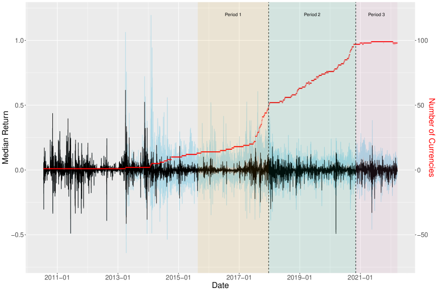
Figure 1: Pointwise median returns over all currencies with $5\%$ and $95\%$ sample quantiles in blue over each date. The number of currencies that have a return at the time is indicated in red. The orange, green, and purple shaded areas correspond to the three periods we analyze closer in Section 5.

For the cryptocurrencies, Figure 1 illustrates the median returns (black) over all cryptocurrencies by date. We can see that in the beginning of the time period, only one currency, namely Bitcoin, was present in the data set. From 2014, we see an incremental increase (red line), while there is a jump up in 2017 and an consecutively faster increase in available cryptocurrencies. We also see that the returns are very different between currencies from 2014 to 2018 (blue), which marks a period of hype leading to a crash in the beginning of 2018. Later, there are large negative spikes corresponding to the many waves of the Covid-19 pandemic. Based on these observations, we divide our data into three periods. The first period ranges from August 2015 (2015-08-22) to the end of 2017 (2017-12-21), while the second period subsequently lasts until November 2020 (2020-11-05). The last period then covers the rest of our data (until 2022-03-20).

Since we are in a time series setup, we include classic covariates based on lagged return in our analysis. Additionally, we employ information specific to each cryptocurrency in 7 external covariates. The five time-series based covariates consist of the one-day lagged return and the lagged 3,7,30, and 60 day return standard deviation. The external covariates are the number of unique active daily addresses (Active_Users), the number of unique addresses that hold any amount of native units of that currency or at least 10 or 100 USD equivalent (Total_Users, Total_Users_USD10,Total_Users_USD100), the supply equality ratio (SER), i.e. the ratio of supply held by addresses with less than $1/10^{7}$ of the current supply to the top 1% of addresses with the highest current supply, the number of initiated transactions (Transactions), and the velocity of supply in the current year (Velocity), which describes the the ratio of current supply to the sum of the value transferred in the last year. See also Table 12 in the appendix for details on the covariates.

Table 2: Summary of Covariates for Different Time Periods

Quantile	Ret	Active_Users	Total_Users	Total_Users_USD100	Total_Users_USD10	SER	Transactions	Velocity	sd_3	sd_7	sd_30	sd_60	CapMrktCurMUSD
Period 1: 5 Currencies
5%	-0.094	7691	233361	7768	32688	0.001	3304	9.321	0.007	0.014	0.022	0.026	17
Median	-0.001	127679	2579591	297029	615602	0.013	49170	33.708	0.036	0.044	0.051	0.055	2611
95%	0.104	324662	9697275	3562101	5930594	0.031	110698	109.281	0.137	0.134	0.123	0.124	185407
Period 2: 15 Currencies
5%	-0.085	3592	95320	5271	16960	0.001	16618	4.668	0.008	0.015	0.024	0.027	70
Median	-0.001	66921	2629309	233835	540993	0.008	128481	16.244	0.034	0.041	0.047	0.049	5008
95%	0.094	179852	8601014	2135275	4469914	0.018	655221	67.849	0.122	0.119	0.111	0.109	99979
Period 3: 77 Currencies
5%	-0.082	2138	533215	15647	41396	0.002	25250	5.255	0.008	0.017	0.026	0.030	233
Median	-0.000	19371	1218761	80236	215034	0.007	137082	15.325	0.035	0.041	0.047	0.049	1794
95%	0.086	76081	2793940	565048	1195791	0.012	424953	53.743	0.111	0.105	0.101	0.096	26105
Full Data: 105 Currencies
5%	-0.089	1857	559862	16964	44887	0.002	19135	5.626	0.009	0.019	0.028	0.033	461
Median	-0.000	15406	1095198	72651	186751	0.006	106286	14.371	0.038	0.045	0.051	0.054	2367
95%	0.095	62448	2389786	434200	917576	0.010	339294	44.627	0.120	0.113	0.108	0.102	21085

Note: values are means of quantiles over all assets contained in the specific time period. CapMrktCurMUSD describe the market cap in Mio. USD and is not included as a covariate due to multicollinearity reasons.

Table 2 gives an overview of the employed covariates and their values in the different time periods. We can see that in Period 1, we have the most extreme returns on average as well as the most extreme lagged standard deviations. This is not surprising looking at the first period (853 days), which arguably marks the most volatile period, with many new currencies being created, as well as the second longest period. In the following period (1050 days), the average median market cap reaches a high as well as the number of users invested in the currencies, indicating that the market is growing while stabilizing more. This is followed by a sharp drop in the market cap for the last, shortest period (500 days), which starts at the beginning of the Covid-19 pandemic. There, the number of active users as well as the SER decreases, indicating that more smaller addresses are pushed off the market, while it is the period with the most currencies.

Given this hugely dynamic cryptocurrency market evolution we distinguish between the three systematically different periods in terms of actively traded currencies and market capitalization. The first one is characterized by a few, rapidly changing currencies and extreme returns and volatilities, while the second period is less extreme and more characterized by a strong increase in median market caps with a few dozens of market components. The third period, in the end, is very short but contains more than five times the number of currencies in comparison to the second period.

3 Methodology

For the prediction of cryptocurrencies, we advocate the use of non-linear machine learning based techniques. In this way, we intend to accommodate the documented large share of speculation (Ghysels and Nguyen, 2019; Baur et al., 2018; Selmi et al., 2018; Glaser et al., 2014) and resulting frequent changes in unconditional volatility which make predictions in this market peculiar. In particular, we focus on generalized random forest methods that are tailored for conditional quantiles of returns and thus allow to forecast the VaR. The flexible but interpretable non-linearity of the approach allows for a direct comparison to standard linear and (G)ARCH-type models. We also argue that the difference in forecasting performance can moreover be employed to detect periods of bubbles and extensive speculation.

Recall that for daily log returns $r_{t}$ the $VaR_{t}$ at level $\alpha\in(0,1)$ conditional on some covariates $x_{t-1}$ is defined as

$$VaR^{\alpha}_{t}(x_{t-1})=\sup_{r_{t}}\left(F(r_{t}|x_{t-1})<\alpha\right)\ ,$$ (1)

where $F$ marks the distribution of $r_{t}$ conditional on $x_{t-1}$. Generally, the conditioning variables could consist of past lagged returns, standard deviations, but also of external (market) information or other assets. We employ these as covariates that are explained in Section 2.

We propose the use of two different types of random forest-based techniques which directly model the conditional VaR in (1). Both build on the classic random forest (Breiman, 2001) which is an ensemble of (decorrelated) decision trees (see e.g. Hastie et al., 2009) for the mean of $r_{t}$. In a decision tree, each outcome $r_{t}$ is sorted into leafs of the tree by binary splits. These splits are performed based on different $x_{t-1}$ components falling above or below specific adaptive threshold values that need to be calculated, for example by the Gini Impurity or MSE-splitting in Classification and Regression Trees (CART) (Breiman et al., 1984), or using other criteria. Finally, the prediction for a new $r_{t}$ is a weighted version of each tree prediction.

In the proposed method that we employ, the generalized random forest (GRF) from on Athey et al. (2019), the random forest split criterion is adapted to mimic the task of quantile regression rather than minimizing a standard mean squared loss criterion for mean regression tasks. Intuitively, the splits in each leaf are conducted by minimizing the Gini-loss, which separates the returns $r_{t}$ as best as possible at different quantiles. To transform the minimizing problem in the splits into a classification task, the response variable $r_{t}$ is transformed in each split to obtain pseudo-outcomes $\rho_{t}=\sum_{k=1}^{K}1\{r_{t}>\theta_{k}\}$, where $\Theta=(\theta_{q_{1}},\dots,\theta_{q_{K}})$ describe a set of $K$ pilot-quantiles of $r_{t}$ in the parent node. These quantiles with levels $\tau=q_{1},\dots,q_{K}$ are then used to calibrate the split. In Athey et al. (2019), this is formally motivated by moment conditions and gradient approximations, but practically, $r_{t}$ is relabeled to a nominal scale depending on the largest quantile it does not exceed. In a final step, the optimal split on a variable component $p$ of $x_{t-1}$ and $j=1,\dots,J$ observations in the parent node is then based on minimizing the above-mentioned Gini impurity criterion for classification. For a separation into two possible leaf sets $v=l,r$, the Gini impurity for one leaf $v$ is $G_{p}^{v}=1-\sum_{k=1}^{K}p_{k,v}^{2}$, where $p_{k,v}=\sum_{j=1}^{J}1\{\rho_{j}=k\textit{ and }\rho_{j}\in v\}/|v|$ is the proportion of $\rho_{j}$ in group $v$ with value $k=1,\dots,K$. The full loss is then an average weighted by leaf size, yielding

$$G_{p}=(|l|G_{p}^{l}+|r|G_{p}^{r})/(|l|+|r|)\ .$$ (2)

We choose the Gini-loss since it is fast and, for certain configurations, produces purer nodes than for example using entropy as a splitting criterion (see e.g Breiman, 1996). This can be particularly helpful when dealing with changing variance (and thus time-varying quantiles) of returns, where we would like to detect single extreme events. For our specific case of $\alpha=0.05$, this implies that values larger than $\theta_{0.05}$ in the parent node are given the value $1$, while others are $0$. Algorithm 1 briefly summarizes the tree building algorithm from Athey et al. (2019) for the quantile version of GRF, where the main differences with regard to the splitting regime in comparison to a classic CART occur in every step the tree is grown.

In addition to that, the outcome that is predicted is not the mean but the $\alpha$-quantile (i.e. $VaR^{\alpha}$), which is done in a way that you do not calculate a weighted average of $r_{t}$ but a weighted average of the empirical CDF $\hat{F}(r_{t}\rvert x_{t-1})=E[1_{\{r_{t}\}|x_{t-1}}]$. Intuitively, log returns $r_{t}$ that have similar $x_{t-1}$ in comparison to a new observation $x_{v}$ receive higher weight in the empirical CDF. Similarity weights $w_{t}(x_{v})$ are measured as the relative frequency on how often $x_{v}$ falls in the same terminal leaf as $x_{t-1}$, for $t=1,\dots,T$, and averaged over all trees for each $x_{t-1}$. This last step was originally introduced by Meinshausen (2006) for random forests.

As a benchmark, we employ the quantile regression forest (QRF) based on Meinshausen (2006). This random forest, however, uses the same splitting regime as the original CART random forest and therefore does not account explicitly for situations where the variance and therefore the quantile changes, as splits are conducted based on a mean-squared error criterion. Since such volatility changes are to be expected for cryptocurrencies in our data, we expect GRF to perform better than QRF, but still include both in the analysis to see potential differences in predictions. Furthermore, GRF uses so-called “honest” trees, meaning that different data (usually the subsampled data for each tree is split again in half) is used for building and “filling” each of the trees with values.

Algorithm 1 Generalized Random Forest - Tree Building

1:Set of “honest”, subsampled observations $X_{T}$ and $R_{T}$; minimum node size $n_{m}$; quantile probabilities $\tau_{K}=(\tau_{1},\dots,\tau_{K})$

2:Growing the tree Create root node $P_{0}$

3:Initialize queue Q with $P_{0}$

4:while Queue is not empty do

5:   Take the oldest element from Q (Parent Node $P$) and remove it from Q

6:   Take a random subsample of $p$ variables index by set $P_{sub}=\{\tilde{1},\dots,\tilde{p}\}$ from $X_{T}$ on which to potentially split and take observations $x^{(P_{sub})}_{i}=(x^{(\tilde{1})}_{i},\dots,x^{(\tilde{P})}_{i})$ from $P$.

7:   Set $loss=\infty$

8:   for h in 1 to p do

9:      Compute quantiles $\theta_{k}$ of $r_{t}$ from parent node $P$ at $\tau_{1},\dots,\tau_{K}$ and compute pseudo outcomes $\rho_{t}=\sum_{k=1}^{K}1\{r_{t}>\theta_{k}\}$ for each $r_{t}\in P$.

10:      For each possible split point in $x^{(h)}$, compute the criterion from Equation (2)

11:      Save loss $s_{h}$ that minimizes this splitting criterion

12:      Save optimal split point $split_{h}$

13:      if $s_{h}<loss$ then

14:         $loss\leftarrow s_{h}$

15:         $ind_{h}\leftarrow h$

16:      end if

17:   end for

18:   if Split on variable $h$ with $split_{ind_{h}}$ succeeded (based on hyperparameters) then

19:      Determine children $C_{1},C_{2}$ according to optimal split

20:      Add both children $C_{1},C_{2}$ to a new daughter node each with corresponding observations left and add these to Q

21:   end if

22:end while

23:One tree of the forest

As benchmarks we further include two types of standard time series methods. We use the CAViaR (CAV) methodology by Engle and Manganelli (2004) and standard quantile regression (Koenker and Hallock, 2001). Both make use of quantile regression (QR) techniques (Koenker and Bassett, 1978) that do not minimize the squared error as in ordinary regression, but use the check function $\rho_{\alpha}(u)=u\left(\alpha-1\{u\leq 0\}\right)$ to minimize $L_{\alpha}(f_{\alpha}(\cdot),x_{t})=\sum_{t=1}^{T}\rho_{\alpha}\left(r_{t}-f_{\alpha}(x_{t})\right)$. For CAV, we use a symmetric absolute value (SAV) component for $f_{\alpha}(\cdot)$, i.e $f_{\alpha}(x_{t},r_{t})=\beta_{1}+\beta_{2}f_{\alpha}(x_{t-1},r_{t-1})+\beta_{3}|r_{t-1}|$, and $f_{\alpha}(r_{t-1},x_{t})=\beta_{4}^{\prime}x_{t}+\beta_{5}r_{t-1}$ for the quantile regression. In contrast to the former methods, they can only capture parametric (non)-linear effects which limits their flexibility.

For comparison, we use a GJR-GARCH(1,1) model (Glosten et al., 1993), a GARCH(1,1) (Bollerslev, 1986) model, a simple historical simulation (Hist), meaning that we predict $VaR^{\alpha}_{t+1}$ at level $\alpha$ as the sample $\alpha$-quantile of the preceding returns in a window of length $K$, i.e. $(r_{t-K+1},\dots,r_{t})$, and one that fits a normal distribution to the sample data and uses the theoretical fitted $\alpha$-quantile as the prediction for $VaR^{\alpha}_{t+1}$ (NormFit). We do not expect the latter to perform well as we have high skewness and excess-kurtosis in the data (see Table 1 in Section 2).

For the proposed random forest-type and all benchmark procedures that allow for additional covariates (GRF, QRF, QR) we include lagged standard deviations (SD) in addition to the lagged level $r_{t-1}$ in the model. We expect these to capture the strongly varying levels of unconditional volatility in particular for the cryptocurrencies in the non-linear structure. Additionally, we also employ the above methods and the GARCH(1,1) model using both the latter covariates as well as the 7 external covariates described in Section 2. These methods are GRF-X, QRF-X, QR-X, and GARCH-X. To establish a fair common ground in used model complexity for the QR, QRF, GARCH-X, and GRF, we select a common set of different SD lags as covariates from an additional Monte-Carlo study. In this, we use the simple SAV-model from Section 4 as a baseline of which the respective specification is tailored to regime changes in the unconditional volatilities as observed form the cryptocurrencies. The model is essentially linear autoregressive of order 1 in the VaR and thus directly yields the VaR as outputs. With this, it is possible to use a MSE-minimizing criterion and select the MSE-minimizing variables for the subsequent simulations and data analysis. Table 3 summarizes the results of this short simulation study, which is why we use 3, 7, 30, and 60 day lagged SD as covariates.

Table 3: MSE Prediction Error for Different Covariate Combinations

Lagged SD (in days)	3	7	30	3 and 7	3 and 30	7 and 30	3, 7 and 30	3, 7, 30, and 60
GRF-MSE	0.124	0.095	0.089	0.075	0.070	0.069	0.059	0.057

MSE prediction error for a simulated SAV-model as in Section 4 for GRF (QRF). The minimum MSE is marked in bold.

To compare the performance of the above methods, we use two types of evaluation approaches. First, we test how well each model predicts the conditional $\alpha$-VaR over the entire out-of-sample horizon using three different sets of evaluation techniques. The simplest way of checking whether a model predicts $VaR^{\alpha}$ correctly over a time horizon is to look at its coverage meaning the number of times $r_{t}$ is smaller than the predicted $VaR^{\alpha}_{t}$. Ideally, this should be exactly $\alpha T$ times. This measure is called Actual over Expected Exceedances (AoE) and is computed as $AoE_{\alpha}=(\alpha T)^{-1}\sum_{t=1}^{T}1\{r_{t}<VaR^{\alpha}_{t}\}$. To test this intuition formally, we employ three tests, the DQ-test from Engle and Manganelli (2004), the Christoffersen-test (Christoffersen, 1998) and the Kupiec-test (Kupiec, 1995). All three tests assume that the forecasts have correct coverage under the null hypothesis. The Kupiec-test is simply the formalization of the above intuition, the Christoffersen-test is robust against serial correlation by assuming that $g_{t}=1\{r_{t}<VaR^{\alpha}_{t}\}\sim Bern(\alpha)$, and the DQ-test additionally accounts for problems with conditional coverage due to clustering of the hits exceedance sequences $g_{t}$ with a regression-based approach. In the empirical analysis, we only report the values of the DQ-test, which is the strictest of the tests, for reasons of clarity. Results for the other tests do not differ substantially and are available upon request from the authors.

Secondly, for comparing the forecast performance of two models 1 and 2 directly, we implement the one-step ahead test for conditional predictive ability (CPA) from Giacomini and White (2006), Theorem 1, that assumes under the null hypothesis that forecasts of model 1 and model 2 have on average equal predictive ability conditional on previous information. As suggested by Giacomini and Komunjer (2005), we use the quantile loss function $L_{\alpha}$ for the test. This tests assumes under the null hypothesis that $H_{0}:\ E\left[\Delta L_{t}|\mathcal{F}_{t-1}\right]=E\left[L_{\alpha}(f_{\alpha}^{(1)},r_{t})-L_{\alpha}(f_{\alpha}^{(2)},r_{t})|\mathcal{F}_{t-1}\right]\equiv E\left[h_{t-1}\Delta L_{t}\right]=0$ and that this loss difference is a martingale difference sequence, where $\mathcal{F}_{t-1}$ contains all information up to time $t-1$ and $f_{\alpha}^{(1)}$ and $f_{\alpha}^{(2)}$ are two competing forecasts. The test statistic is computed using a Wald-type test with a set of factors $h_{t-1}$ that can possibly predict the loss difference $\Delta L_{t}$ and is $\chi^{2}_{q}$-distributed under $H_{0}$. More specifically, we choose $h_{t-1}=(1,\Delta L_{t-1})$ (i.e. $q=2$), i.e. using the lagged loss difference and an intercept as predictors in a linear regression with parameter $\beta_{0}$ for the simulation and application.

4 Simulation

In this section, we study the finite sample forecast performance in quantiles for true DGPs of standard stock-type dynamics as well as for set-ups of cryptocurrency type. Overall, we find that, as expected, GRF performs best in all settings, in particular in settings which are designed to mimic the cryptocurrency behaviour over time but also in those similar to stock index behaviour. For QRF, the performance is entirely different, at least for the chosen parsimonious model specification and the relatively short estimation intervals.

We study two different types of DGPs. The first one is a standard GARCH(1,1) process, i.e

$$r_{t} =z_{t}\sigma_{t}$$ (3)

$$\sigma^{2}_{t} =\omega+\beta_{0}\varepsilon^{2}_{t-1}+\beta_{1}\sigma^{2}_{t-1}\ ,$$ (4)

where the parameters are estimated on the full Bitcoin data to mimic the behavior of cryptocurrencies (with $z_{t}\sim N(0,1)$). We denote this setting as sim GARCH Bitcoin fit. Moreover, we also consider the specification with $\beta_{0}=0.1$, $\beta_{1}=0.8$, $\omega=10^{-4}$ and $z_{t}\sim N(0,1)$ (sim GARCH) and with $z_{t}$ as $t_{5}$-distributed (sim GARCH t), which corresponds to standard stock index data. Secondly, for the Sim SAV-Model setting, we fit a symmetric absolute value (SAV) model to normal returns, i.e.

$$\textit{VaR}_{t+1}=\gamma_{0}+\gamma_{1}\textit{VaR}_{t}+\gamma_{2}|r_{t}^{(\textit{init})}-\gamma_{3}|\ ,$$ (5)

with $r_{t}^{(\textit{init})}\sim N(0,\sigma_{t}^{2})$ and $\dfrac{\sigma_{t}}{65}\sim\chi^{2}_{2}$, where new draws of $\sigma_{t}$ are only taken every 100 observations, keeping $\sigma_{t}$ constant meanwhile. We then generate the final return as $r_{t}\sim N\left(0,\dfrac{\widehat{VaR}_{t}}{\Phi(\alpha)^{-1}}\right)$ from the fitted SAV-model, where $\Phi(\alpha)^{-1}$ is the quantile function of a standard normal variable. We do this to obtain returns that have exactly the VaR that we obtained from the SAV model before.

Table 4: Simulation: $5\%$ VaR

Rolling Window	$l=500$				$l=1000$
	DQ	Kupiec	Christoffersen	AoE		DQ	Kupiec	Christoffersen	AoE
Sim GARCH Normal
QRF	$0.940$ $(0.008)$	$0.325$ $(0.200)$	$0.200$ $(0.275)$	1.185		$0.725$ $(0.063)$	$0.160$ $(0.377)$	$0.090$ $(0.393)$	1.148
GRF	$0.495$ $(0.163)$	$0.000$ $(0.583)$	$0.015$ $(0.549)$	1.040		$0.225$ $(0.317)$	$0.020$ $(0.547)$	$0.030$ $(0.525)$	1.030
QR	$0.760$ $(0.048)$	$0.085$ $(0.441)$	$0.090$ $(0.438)$	1.095		$0.305$ $(0.270)$	$0.040$ $(0.537)$	$0.040$ $(0.496)$	1.042
Hist	$0.835$ $(0.045)$	$0.015$ $(0.554)$	$0.195$ $(0.365)$	1.047		$0.630$ $(0.110)$	$0.060$ $(0.490)$	$0.195$ $(0.368)$	1.030
NormFit	$0.740$ $(0.071)$	$0.040$ $(0.551)$	$0.205$ $(0.329)$	1.006		$0.555$ $(0.130)$	$0.065$ $(0.475)$	$0.195$ $(0.345)$	1.001
CAV	$0.785$ $(0.051)$	$0.025$ $(0.514)$	$0.010$ $(0.545)$	1.073		$0.275$ $(0.286)$	$0.055$ $(0.513)$	$0.025$ $(0.511)$	1.032
GARCH(1,1)	$0.445$ $(0.209)$	$0.030$ $(0.511)$	$0.155$ $(0.394)$	1.046		$0.205$ $(0.327)$	$0.055$ $(0.531)$	$0.095$ $(0.428)$	1.028
Sim GARCH t
QRF	$0.920$ $(0.018)$	$0.315$ $(0.203)$	$0.210$ $(0.277)$	1.188		$0.655$ $(0.085)$	$0.175$ $(0.348)$	$0.100$ $(0.399)$	1.162
GRF	$0.435$ $(0.188)$	$0.010$ $(0.579)$	$0.025$ $(0.537)$	1.029		$0.260$ $(0.341)$	$0.030$ $(0.522)$	$0.020$ $(0.518)$	1.022
QR	$0.770$ $(0.060)$	$0.130$ $(0.407)$	$0.105$ $(0.407)$	1.109		$0.275$ $(0.303)$	$0.040$ $(0.507)$	$0.035$ $(0.468)$	1.049
Hist	$0.725$ $(0.077)$	$0.020$ $(0.573)$	$0.200$ $(0.360)$	1.036		$0.580$ $(0.121)$	$0.115$ $(0.440)$	$0.185$ $(0.334)$	1.016
NormFit	$0.695$ $(0.090)$	$0.310$ $(0.271)$	$0.370$ $(0.220)$	0.839		$0.550$ $(0.155)$	$0.340$ $(0.275)$	$0.370$ $(0.239)$	0.817
CAV	$0.525$ $(0.135)$	$0.010$ $(0.523)$	$0.010$ $(0.542)$	1.059		$0.175$ $(0.331)$	$0.055$ $(0.499)$	$0.040$ $(0.502)$	1.032
GARCH(1,1)	$0.405$ $(0.232)$	$0.135$ $(0.381)$	$0.210$ $(0.316)$	0.893		$0.270$ $(0.308)$	$0.200$ $(0.368)$	$0.220$ $(0.344)$	0.862
Sim SAV-Model
QRF	$0.960$ $(0.010)$	$0.315$ $(0.188)$	$0.180$ $(0.265)$	1.187		$0.735$ $(0.071)$	$0.150$ $(0.352)$	$0.115$ $(0.413)$	1.158
GRF	$0.495$ $(0.148)$	$0.005$ $(0.571)$	$0.025$ $(0.570)$	1.047		$0.210$ $(0.317)$	$0.040$ $(0.518)$	$0.035$ $(0.548)$	1.048
QR	$0.895$ $(0.024)$	$0.050$ $(0.435)$	$0.045$ $(0.452)$	1.102		$0.310$ $(0.234)$	$0.045$ $(0.490)$	$0.045$ $(0.530)$	1.064
Hist	$0.290$ $(0.220)$	$0.035$ $(0.595)$	$0.070$ $(0.523)$	1.047		$0.165$ $(0.353)$	$0.070$ $(0.525)$	$0.080$ $(0.496)$	1.048
NormFit	$0.215$ $(0.360)$	$0.040$ $(0.539)$	$0.110$ $(0.502)$	0.994		$0.145$ $(0.418)$	$0.080$ $(0.501)$	$0.070$ $(0.474)$	0.999
CAV	$0.775$ $(0.053)$	$0.030$ $(0.525)$	$0.030$ $(0.563)$	1.067		$0.235$ $(0.289)$	$0.045$ $(0.527)$	$0.045$ $(0.563)$	1.038
GARCH(1,1)	$0.135$ $(0.338)$	$0.030$ $(0.567)$	$0.065$ $(0.528)$	1.021		$0.065$ $(0.469)$	$0.045$ $(0.546)$	$0.040$ $(0.524)$	1.018
Sim GARCH Bitcoin fit
QRF	$0.875$ $(0.018)$	$0.325$ $(0.200)$	$0.200$ $(0.275)$	1.185		$0.585$ $(0.110)$	$0.160$ $(0.377)$	$0.090$ $(0.393)$	1.148
GRF	$0.255$ $(0.303)$	$0.000$ $(0.583)$	$0.015$ $(0.549)$	1.040		$0.160$ $(0.454)$	$0.020$ $(0.547)$	$0.030$ $(0.525)$	1.030
QR	$0.635$ $(0.095)$	$0.085$ $(0.441)$	$0.090$ $(0.438)$	1.095		$0.170$ $(0.380)$	$0.040$ $(0.537)$	$0.040$ $(0.496)$	1.042
Hist	$0.600$ $(0.102)$	$0.015$ $(0.554)$	$0.195$ $(0.365)$	1.047		$0.385$ $(0.269)$	$0.060$ $(0.490)$	$0.195$ $(0.368)$	1.030
NormFit	$0.540$ $(0.159)$	$0.040$ $(0.551)$	$0.205$ $(0.329)$	1.006		$0.330$ $(0.299)$	$0.065$ $(0.475)$	$0.195$ $(0.345)$	1.001
CAV	$0.970$ $(0.007)$	$0.375$ $(0.178)$	$0.280$ $(0.224)$	0.814		$0.655$ $(0.055)$	$0.305$ $(0.236)$	$0.270$ $(0.273)$	0.791
GARCH(1,1)	$0.230$ $(0.319)$	$0.030$ $(0.536)$	$0.180$ $(0.399)$	1.054		$0.100$ $(0.458)$	$0.040$ $(0.545)$	$0.080$ $(0.438)$	1.032

The table displays rejection rates of t-tests of empirical quantile levels against the nominal level of $5\%$ for DQ-, Kupiec- and Christoffersen-tests and mean p-values in parentheses. Thus higher p-values and lower rejection rates indicate better model performance. The GARCH case uses predictions from the QMLE-fit of a GARCH(1,1) specification with normally distributed errors and can therefore be seen as an oracle for the GARCH-simulated specifications.

For all settings, we generate 2000 return observations and forecast the one-step ahead VaR over the different rolling window lengths $l=500,1000$. We repeat this generation process 200 times for $\alpha=0.01$ and $\alpha=0.05$. For comparison of the different methods described in Section 3, we use the DQ-test, the Kupiec test, the Christoffersen-test, and the AoE. Note that for all tests, we present aggregate results from two-sided t-tests of the empirical versus the nominal coverage. The results are therefore rejection rates of t-tests against the nominal level of 5%. Therefore, a lower rejection rate and higher mean p-values (in parentheses) indicate better performance. For GRF, QRF, and QR, we use a common set of lagged covariates as described at the end of Section 3.

Table 4 summarizes the results of the simulation for the 5% $VaR$. According to the more advanced $DQ$- and Christoffersen-tests for evaluation, GRF consistently outperforms the other methods in almost all cases, indicating superior predictive quality. This is very much in contrast to the QRF which is consistently dominated by the other models. For the Sim GARCH and Sim GARCH t cases which mimic standard stock indices, the performances of GRF, CAV and QR appear in a similar range with mostly advantages for GRF in particular for smaller sample sizes. This holds generally for normally distributed as well as heavy tailed innovations which lead to similar results also in magnitude of the rejection rates. As expected, forecasting performance increases throughout all models with larger estimation windows, though with CAV often profiting the most from the larger sample sizes. For these settings with GARCH as the true DGP, the performance of the GARCH model serves as an oracle reference. In the t-innovation case, it has coverage problems and GRF is even able to outperform it in Christoffersen-tests.

For the Sim SAV Model and the Sim GARCH Bitcoin fit the situation, however, differs substantially. In these cryptocurrency-like cases, the GRF clearly dominates the QR and CAV particularly strongly in the small 500 observations setting. Considering our application where only a relatively small time span is available, this seems crucial. Moreover, CAV runs into coverage problems according to the AoE results which even deteriorate for larger sample sizes for Sim GARCH Bitcoin fit. In the latter case, the GRF rejection rates are close to the GARCH benchmark while the strong conditional dependence structure in the tails of the Sim SAV Model setting shows that for such extreme cases, the unconditional coverage of GRF is still excellent, but the conditional coverage measured by the DQ-test is only average among all models for the larger estimation samples and even below for the smaller ones. These relative findings generally prevail for the 1% VaR forecasts, but absolute performance is generally worse for all methods, especially with a smaller rolling window of 500 (see Table 16 in the appendix.). Intuitively, this finding is reasonable, since relevant observations for the 1% level should in theory only occur in 5 of the 500 observations, making it harder for the data-driven methods to predict such unlikely events.

Additionally, we conduct direct pairwise comparison tests between the superior random forest type method GRF against the best performing non-oracle other parametric methods via CPA-tests for each scenario. The respective results are reported in Table 5. In the majority of cases, GRF outperforms its competitors on average, however, mean p-values are mostly not significant. For example, GRF has a smaller loss (i.e. quantile loss) than QR in about 90% of the forecasts (aggregated over all runs) but a mean p-value of 0.298, which would not qualify as a significant out-performance (on average). This of course does not mean that the test never rejects but is likely be caused by high variances in the p-values over different simulation runs. Furthermore, the competing methods are also slightly improving with window length, which further implies that GRF can deal better with a smaller training time frame.

Table 5: CPA-tests on Predictions of $5\%$ VaR for Different Window Lengths and Different Models

Rolling Window	$l=500$				$l=1000$
GRF vs:	QR	Hist	CAV		QR	Hist	CAV
Sim GARCH Normal
Mean P-Value	${0.429}$	${0.351}$	${0.334}$		${0.491}$	${0.388}$	${0.463}$
No. P-Values $<0.1$	${34}$	${55}$	${50}$		${24}$	${44}$	${27}$
GRF-Performance	${0.780}$	${0.755}$	${0.847}$		${0.501}$	${0.744}$	${0.659}$
Sim GARCH t
Mean P-Value	${0.392}$	${0.382}$	${0.396}$		${0.431}$	${0.397}$	${0.446}$
No. P-Values $<0.1$	${43}$	${40}$	${34}$		${30}$	${37}$	${15}$
GRF-Performance	${0.732}$	${0.707}$	${0.692}$		${0.439}$	${0.717}$	${0.529}$
Sim SAV-Model
Mean P-Value	${0.298}$	${0.311}$	${0.374}$		${0.471}$	${0.381}$	${0.448}$
No. P-Values $<0.1$	${53}$	${63}$	${42}$		${26}$	${50}$	${22}$
GRF-Performance	${0.903}$	${0.279}$	${0.775}$		${0.657}$	${0.321}$	${0.658}$
Sim GARCH Bitcoin fit
Mean P-Value	${0.429}$	${0.351}$	${0.001}$		${0.491}$	${0.388}$	${0.003}$
No. P-Values $<0.1$	${34}$	${55}$	${200}$		${24}$	${44}$	${199}$
GRF-Performance	${0.780}$	${0.755}$	${0.995}$		${0.501}$	${0.745}$	${0.994}$

Note: the table displays CPA-tests for $5\%$ one-day ahead VaR-forecasts of the best performing random forest type techniques GRF in Table 4 versus the best parametric time series models. We report mean p-values, the number of significant p-values over 200 iterations and the rate at which GRF outperforms the competing method (i.e. a value of 0.8 means that GRF has a smaller error loss than the competing method in 80% of the rolling window forecasts over all runs). Low p-values paired with performance rates larger than 0.5 indicate that GRF outperforms the competing methods.

5 Results

In this section, we highlight the advantages from using non-linear machine learning-based methods for forecasting the VaR of cryptocurrencies. In particular, we show for a large cross-section of more than 100 cryptocurrencies that the proposed random forest method GRF yields superior performance across a wide range of different types of cryptocurrencies and different time periods. Investigating the underlying drivers, we illustrate that the non-linear model predictions excel especially for assets that are frequently traded by a large amount of different users, and for more volatile assets and times.

More specifically, we predict the $5\%-\textit{VaR}$ as a key quantity in risk management for our comprehensive set of cryptocurrencies. In an extensive out-of-sample forecasting study, we compare the random forest-based machine learning methods to standard linear time series and GARCH-type models including approaches with exogenous asset information in covariates. The prediction performance is assessed with the DQ-test to obtain an overall aggregate picture on the realized coverages as well as pairwise CPA-tests across different time periods and types of cryptocurrencies. Based on these findings, we focus our analysis on three important selected currencies comprising Bitcoin (btc) as the largest currency by far regarding market cap, Tether (usdt) as a stablecoin with lower volatility, and Cardano (ada) as a currency specifically allowing for smart contracts. For these we also consider predicted loss series by CPA-tests and variable importance measures to uncover important drivers. We furthermore identify single events that majorly affect the predictive ability of the procedures.

5.1 Aggregated Forecasting Performance

In this section, we provide results on aggregate forecast performance of the different modeling approaches over all cryptocurrencies.

5.1.1 Backtesting

Table 6: Medians of P-Values for DQ-Tests in Different Time Periods

Period	GRF	QRF	QR	CAV	GJR-GARCH	Hist	GRF-X	QRF-X	QR-X	GARCH-X
1	0.16	0.29	0.08	0.06	0.03	0.00	0.00	0.00	0.00	0.00
2	0.27	0.09	0.06	0.27	0.17	0.08	0.13	0.06	0.00	0.00
3	0.18	0.05	0.07	0.03	0.30	0.01	0.20	0.10	0.00	0.03

Note: Higher median p-values indicate correct conditional coverage according to the DQ-test. Periods correspond to the times indicated in Figure 1.

Table 7: Medians of P-Values for DQ-Tests Sorted by SER in Different Time Periods

Group	GRF	QRF	QR	CAV	GJR-GARCH	Hist	GRF-X	QRF-X	QR-X	GARCH-X
Period 1
High	0.16	0.92	0.00	0.00	0.12	0.00	0.01	0.00	0.00	0.00
Low	0.13	0.28	0.10	0.10	0.02	0.00	0.00	0.00	0.00	0.00
Period 2
High	0.16	0.08	0.20	0.19	0.11	0.08	0.13	0.07	0.00	0.00
Low	0.29	0.10	0.06	0.31	0.25	0.10	0.32	0.06	0.00	0.09
Period 3
High	0.47	0.05	0.22	0.11	0.21	0.01	0.51	0.12	0.00	0.00
Low	0.07	0.04	0.03	0.02	0.32	0.00	0.18	0.07	0.00	0.06

Note: The currencies are divided into two groups based on specific covariate values for each time period. The groups are constructed to best separate the sorted covariate values of the currencies. They are therefore separated around their steepest decay to obtain two groups with homogeneous SER values. Detailed plots for the group separation can be found in Figure 10, column 1. The remaining details correspond to Table 6.

We analyze the three fundamentally distinct periods 08/2015–12/2017, 01/2018–11/2020, and 12/2020–03/2022 of the cryptocurrency market which differ according to the number of actively traded currencies, the market capitalization and the overall market situation (see Section 2). We thus analyze each period separately, with a focus on the last period 3 in the aggregate, where the number of available currencies is relatively high. Given the largely different market situations, we refrain from reporting results for the full time period. We assess the performance of VaR forecasts by their conditional coverage and the dependence structure of exceedances, which we test with the DQ-test (see Section 3 for details). This test is the most strict of all backtests, conditioning on past information, and therefore most accurately captures the coverage abilities of the procedures. The results over the different time periods for the 5% VaR-predictions are shown in Table 6. We can see that depending on the time period, the median p-values vary strongly, which is not surprising giving the different characteristics of each period and the increasing number of cryptocurrencies in the later periods. In general, GRF is the only method with median values consistently over the 10% level, indicating that it is the most consistently calibrated forecasting method. The QRF performs extremely well in the first time period, but rejects the test often in the third period. Adding external covariates as listed in Table 2 does not improve performance and in general leads to substantially lower p-values especially for the QR. Only in the final third period, adding external covariates increases the p-values slightly for the GRF and substantially for the QRF (GRF-X, QRF-X). This indicates that those extra covariates are not necessarily predictive for extreme returns, or rather that the existing measures such as lagged returns and SD comprise the information already quite well. Compared to its non-forest counterparts, only CAV and GJR-GARCH can partly keep up with GRF. GJR-GARCH has higher median p-values than GRF in the third period, which is the shortest and which contains the most currencies. It is also marked by less extreme returns and a large reduction in active users (see Table 2), which could indicate that the forest methods excel in particular in highly volatile periods, when large shifts in the market are present. On the other hand, CAV has a similar, slightly worse performance in the second period while performing much worse than GRF in the other periods. This highlights the inability of the parametric methods to adapt to rapidly changing situations such as in Period 1 and 3. QR, Hist, and GARCH-X are all fully dominated by GRF throughout the three time periods as expected, as QR can only incorporate changes linearly, and GARCH-X and Hist serve as simple baselines. Additionally, when checking the unconditional (median) coverage represented as the ratio of exceedances relative to the expected ones, random forest-type methods also show superior performance over standard GARCH-type methods, which have quite low coverage in all (GARCH-X) or the first period (GJR-GARCH).

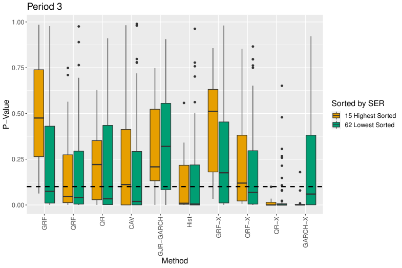
Figure 2: Boxplots of p-values of DQ-tests over all cryptocurrencies contained in Period 3 separated into groups with high vs low SER for every method. For details on the groups, see Table 7. The dashed horizontal line depicts a level of 0.1.

We investigate Period 3, which contains 77 cryptocurrencies, more in detail, especially with regard to how conditional coverage is characterized by external information. For this, we split the currencies into two groups depending on the value of the SER, which characterizes the concentration of supply to users. A low SER consequently implies that most supply is concentrated on a few, large users, often indicating a more stable currency. Figure 2 depicts boxplots over p-values of DQ-tests for each group and procedure in Period 3. GRF(-X) performs particularly well for the groups with a high SER, which arguably are more prone to speculations during hype/bubble periods due to the large amount of supply held by many small addresses. For the (arguably) more stable addresses with a smaller SER, GJR-GARCH has higher p-values, followed by GRF-X, which has the most consistent performance in this period. This is in contrast to CAV, QR, or QRF, which are always outperformed by GRF(-X), as well as the simple baselines Hist and GARCH-X. For details on all time periods and groups according to the different observable factors active users and lagged standard deviation, see Table 13 in the appendix.

5.1.2 Direct Pairwise Forecast Comparisons

In addition to assessing the coverage performance, we conduct pairwise CPA-tests for all considered methods in the three different specified time periods over all cryptocurrencies. The results of the tests are contained in Table 8 and Figure 4. Note that the CPA-tests require the rolling window length to be smaller than the out-of-sample forecast window to produce valid results. Therefore the results from the shortest period Period 3, where both window sizes are equal to 500 might have less power. Thus by construction, for the only recently introduced cryptocurrencies in period 3, the out-of-sample size is too low for the CPA-tests to have high power. Therefore, we additionally look at the direct comparisons of predicted losses (as suggested by Giacomini and White (2006), Section 4), where we compare in the loss series how often GRF is better, i.e. has a smaller loss, than its competitors (GRF-Performance). Note that a value of one thus indicates that GRF has a smaller predicted loss over the full loss series.

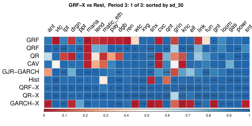
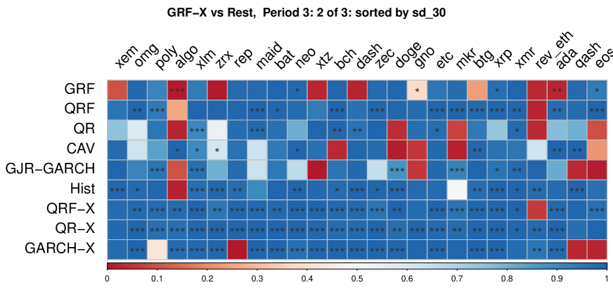
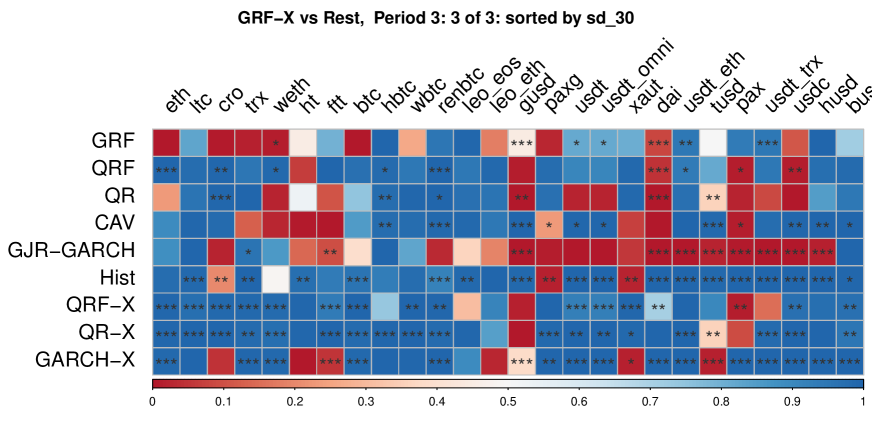
Figure 9: Overview of results for CPA-tests of GRF-X vs. all other methods for cryptocurrencies in the third period ordered by 30 day lagged standard deviation from highest to lowest, left to right. The color of each box indicates the performance of GRF-X, with 1 indicating that GRF-X has a smaller predicted loss in 100% of cases. *, **, *** indicate significance on a level of 10%, 5%, and 1%.

In general, GRF performs better than its competitors for a majority of crypotocurrencies over all time periods. Table 8 summarizes the results. We can see that QRF is almost always outperformed, and for around 50% of cryptocurrencies, losses are even significantly smaller. This is not surprising, as QRF has a similar structure to GRF while not being tuned to predict the quantiles directly. Thus, we expect it to be less sensitive to changes that only affect the quantile of the return distribution, for example large shock events. The same holds for the GARCH-X and Hist, which are clearly outperformed by the GRF, as well as the QR-X and QRF-X. Adding exogenous information in covariates as part of the non-linear GRF (i.e. GRF-X) is better especially in later periods (see Figure 9 in the appendix). This is interesting, since the other methods cannot benefit as much as GRF from additional covariates. Generally, for cryptocurrencies, the non-parametric form of the GRF helps to extract information from exogenous covariates in contrast to standard parametric methods such as QR and GARCH. As GRF accounts specifically for the quantiles in the random forest splitting function, this helps to also favorably integrate additional covariates $X$ in contrast to QRF. Overall, however, both GRF-procedures seem to perform very similarly, especially in pairwise comparisons. For full results of the GRF-X, see Table 14 and Figure 9 in the appendix. While CAV, QR, and GJR-GARCH are outperformed over the majority of cryptocurrencies, only 20% to 50% of these out-performances reach significance. In subsection 5.2, we will focus on specific cryptocurrencies for a more in-depth understanding.

Table 8: Performance and Significance of CPA-tests Over Different Time Periods for GRF Without Additional Covariates

GRF vs.:	QRF	QR	CAV	GJR-GARCH	Hist	GRF-X	QRF-X	QR-X	GARCH-X
Share of GRF With Better Performance
Period 1	1.00	0.80	0.80	1.00	1.00	0.60	1.00	1.00	1.00
Period 2	1.00	0.73	0.87	0.80	0.93	0.40	1.00	1.00	1.00
Period 3	0.92	0.68	0.71	0.64	0.90	0.44	0.92	0.96	0.70
Full Data	0.91	0.74	0.75	0.71	0.82	0.44	0.90	0.97	0.72
Share of GRF With Significantly Better Performance
Period 1	0.40	0.40	0.20	0.20	1.00	0.00	1.00	1.00	0.60
Period 2	0.53	0.33	0.27	0.33	0.73	0.00	1.00	0.87	0.67
Period 3	0.43	0.21	0.23	0.19	0.51	0.09	0.74	0.78	0.53
Full Data	0.41	0.31	0.24	0.18	0.41	0.12	0.69	0.83	0.54

The top part shows summary values that are shares over all cryptocurrencies in the respective time period. It describes the number of times that GRF had a better performance (i.e. more than 50% of predicted losses by the CPA test were smaller for the GRF) relative to all crytpocurrencies (in that period), and the number of times that GRF was significantly better (at least at a 10% level) as judged by the CPA test over all crytpocurrencies (in that period). The bottom part shows the detailed results of CPA-tests with the color of each box indicating the performance of GRF. Blue signifies a performance of 1, meaning that GRF has a smaller predicted loss in 100% of cases. *, **, *** shows significance on a level of 10%, 5%, and 1%. The values are ordered by 30 day lagged standard deviation from highest to lowest (top/left to bottom/right).

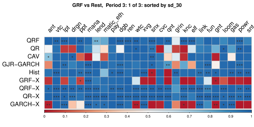
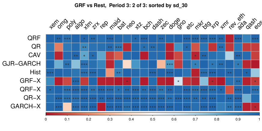
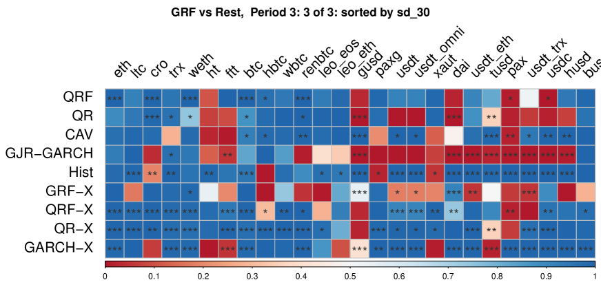
Figure 4: Overview of results for CPA-tests of GRF vs. all other methods for cryptocurrencies in the third period ordered by 30 day lagged standard deviation from highest to lowest, left to right. The color of each box indicates the performance of GRF, with 1 (blue) indicating that GRF has a smaller predicted loss in 100% of cases. *, **, *** indicate significance on a level of 10%, 5%, and 1%.

When considering the single time periods, it is notable how for Period 1 and 2 (bottom part of Table 8), GRF(-X) is constantly outperforming the other methods for most cryptocurrencies, and only has somewhat worse performance for doge and the stablecoins, although these are insignificant (see below). For the first two periods, QR is maybe the most competitive of the other methods, while there is a general tendency for the classic methods to perform worse with higher volatility of returns, which can be seen in Table 8 for Period 2 where the currencies are ordered from highest 30 day lagged SD on the left to the lowest on the right. This becomes more apparent in Period 3, where we deal with much more cryptocurrencies (77) and a much shorter time horizon (500 out-of-sample observations). Here, methods such as GJR-GARCH and QR are on par with GRF or even better when looking at low-volatility (partly regulated) stablecoins such as pax, gusd, tusd, dai, and usdt with its derivatives (e.g. usdt_eth,usdt_trx). CAV, on the other hand, is only rarely better here (as indicated by CPA tests), while being significantly outperformed for important and large assets such as btc, ada, xlm, and most stablecoins where the QR and GJR-GARCH performed well.

To highlight the specific properties of currencies where GRF outperforms the other methods, we split the assets into two groups. The first group (Group_low) contains assets where GRF performance is low in comparison to the three other methods that were able to compete in some cases with GRF, namely QR, CAV, and GJR-GARCH. We add an asset into that group when at least two of the methods outperform GRF (in terms of loss difference) for that asset, separately for each time period. All other assets are sorted into the second group (Group_high), indicating high performance of GRF. Table 9 summarizes the results over these groups for each time period and covariate. In each group, we take the mean over all cryptocurrencies of median values for each covariate. We then divide Group_low by Group_high. For example, An SER of 0.15 in Period 3 indicates that cryptocurrencies in Group_low have, on average, a median SER that is only 15% to that of Group_high, or in other words, the median SER for Group_high is around $6.7=\dfrac{1}{0.15}$ times higher than that of Group_low on average. We see that covariates of cryptocurrencies for which GRF performs better have much higher volatility (especially for the second and third period), a much higher SER, indicating a larger concentration of supply at a lot of small addresses, a higher market capitalization, a lower rate of turnover (Velocity), and more active and total users. To summarize, this confirms the observation that GRF performs better for assets with highly varying returns that are traded by a large amount of users, which could thus also be prone to speculation. On the other side, methods such as QR or GJR-GARCH are better with more stable currencies that are used more as a hedging device (e.g. stablecoins). This confirms our findings from the backtests in Section 5.1.1, where GRF excels in particular for currencies with high SER values, high volatility, and a large number of active users.

Table 9: Difference Between Covariates of Cryptos Where GRF is Better vs. Worse

	Period 1	Period 2	Period 3	Full Data
Ret	1.20	0.16	1.05	0.92
Active_Users	0.34	0.15	0.26	0.34
Total_Users	0.79	0.18	0.13	0.15
Total_Users_USD100	0.22	0.17	0.27	0.35
Total_Users_USD10	0.41	0.17	0.19	0.25
CapMrktCurUSD	0.08	0.11	0.37	0.33
SER	1.07	0.50	0.15	0.21
Transactions	0.42	0.04	1.20	1.53
VelCur1yr	4.68	3.11	1.48	1.43
sd_3	0.89	0.52	0.59	0.58
sd_7	0.91	0.54	0.59	0.57
sd_30	0.90	0.52	0.59	0.58
sd_60	0.91	0.54	0.58	0.57

Note: Values are shares of groups of cryptocurrencies where at least two of CAV, QR, and GJR-GARCH have better CPA-performance than GRF divided by the remaining rest. Raw values before division are mean values over all cryptocurrencies for the median of each covariate in the respective time period. A value smaller than 1 indicates that currencies where GRF performs better have a higher average median values of the respective covariate than the rest of the currencies.

5.2 Extension: In-Depth Analysis of Specific Classes of Assets

To identify which specific events drive the performance of these methods, we analyze the predicted loss series of CPA tests over the full horizon of availability for the three cryptocurrencies Bitcoin, Cardano, and Tether separately. We furthermore show which covariates are important over the full data and specific time periods using variable importance measures of GRF-X.

We choose Bitcoin since it is the largest currency by market cap, with the longest data availability, Tether as the largest stablecoin by daily volume and market cap, and Cardano as a fairly new (i.e. fewer observations), however large currency (again by market cap), which can be used for smart contracts, identity verification, or supply chain tracking. Since we deal with VaR-predictions, the initial loss function is the quantile loss with a quantile $\alpha=0.05$.

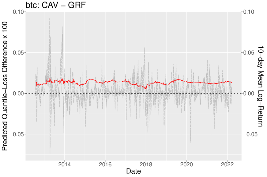
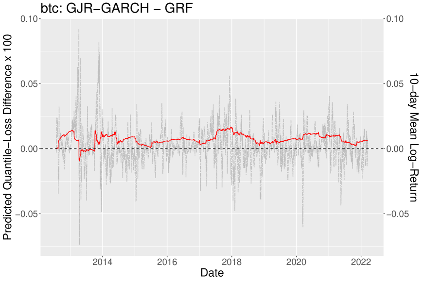
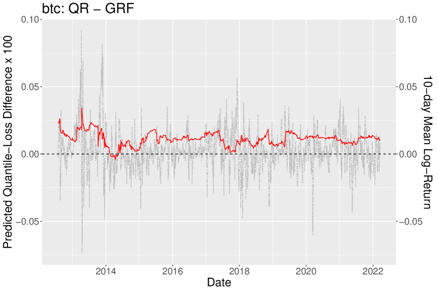
Figure 5: Rolling 180-day mean of predicted loss difference series (red) of $h_{t}\hat{\beta}_{0}$ of CPA tests on Bitcoin (btc) predicted 5% VaR with $l=500$ for GRF vs. CAV (left), GJR-GARCH (right), and QR (bottom center) with rolling mean 10-day log-returns in grey. A positive predicted loss difference indicates that the prediction error of GRF is smaller than of the compared method.

First, we look at Bitcoin (btc), the largest and most popular currency, where GRF largely outperforms QR, CAV, and GJR-GARCH in the CPA-tests. Figure 5 shows the predicted loss difference for each of the different methods. GRF outperforms the other methods consistently for most time frames. This is most likely due to the specific tailoring of the methodology to quantiles, as it outperforms QRF (not plotted) consistently here. For the parametric methods GJR-GARCH and QR, there are two short time periods where they have a smaller loss. For GJR-GARCH, this happens in the very beginning of the out-of-sample periods in April 2013, where btc crashed with negative log-returns of up to $-0.66$. Since this was the first drop of that magnitude for btc, GRF, as a forest based-method, had never seen such an extreme event, therefore could have technically not predicted it. GJR-GARCH, on the other hand, as a parametric method, has no range restriction in that regard. In the following crashes, GRF correctly predicts these extreme events better than GJR-GARCH, which is visible from the loss series. For QR, the short time frame is only caused by the predictions of the CPA test itself, while actual losses are smaller for GRF.

Secondly, as summarized on the left in Figure 6, we look at Cardano (ada), a large and fairly new currency offering e.g. smart contracts or supply chain tracking. There, GRF is significantly outperforming GJR-GARCH and CAV, while being slightly better than QR, although not reaching a significant level. This lack of power for QR is likely due to the small out-of-sample size (roughly 1000) for the fairly new asset compared to the training window of $l=500$. Again, we can see that around the most extreme spike in March 2020, GJR-GARCH is slightly better, as GRF has not yet seen such an extreme event, therefore is not able to correctly predict the size of the loss. One normal solution would be to increase the training length, which is not possible in this case with a fairly new currency. Interestingly, in the later extreme events in May 2022, GRF increases in performance compared to GJR-GARCH, confirming the challenge with lacking training data.

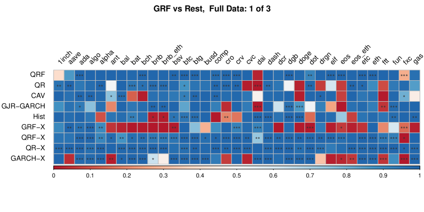
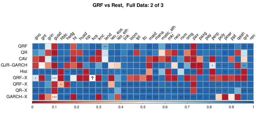
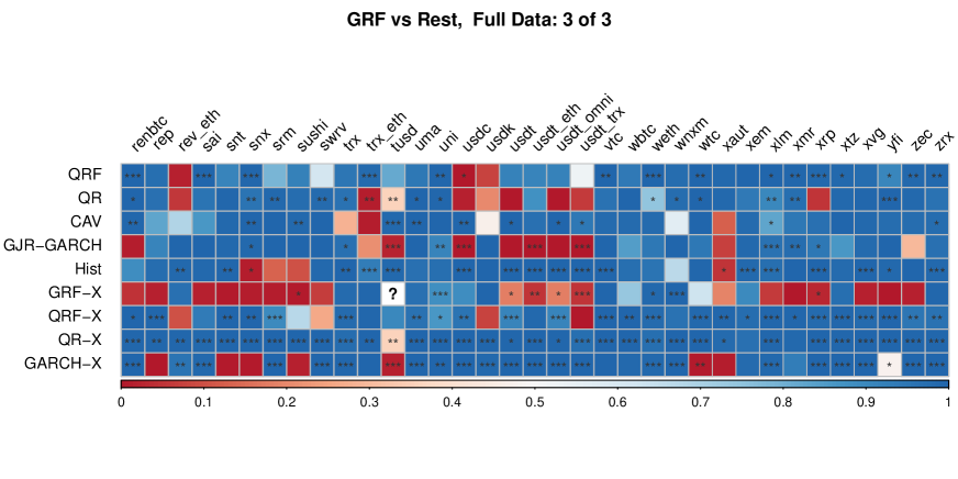
Figure 13: Overview of results for CPA-tests of GRF vs. all other methods for cryptocurrencies for the full data set ordered alphabetically. The color of each box indicates the performance of GRF, with 1 indicating that GRF has a smaller predicted loss in 100% of cases. *, **, *** indicate significance on a level of 10%, 5%, and 1%.

Finally, we also look more closely at Tether (usdt) as the largest stablecoin that is roughly bound to the USD. The right part of Figure 6 shows the 30-day rolling means of the predicted loss differences. Notably, the rolling loss difference and rolling mean-return are already around 10 times smaller than those of btc or ada, indicating that usdt substantially differs from the other two currencies. While the losses of QR are very similar to those of GRF, CAV is significantly worse. Only GJR-GARCH consistently has lower predicted losses than GRF, although they are deemed not significant by the CPA tests (see Figure 13 in the appendix for detailed results for the full time frame). We can see, however, that for the relatively rare tail events in 2017, which are still not too extreme, there is some variation in the predicted loss difference. For the first event that is quite extreme, GJR-GARCH reacts too late, and only the second event is correctly detected by GJR-GARCH, as there is some limited information of anticipation. In general, GRF tends too overshoot less in these situations, which is also reflected in the DQ-tests, where GRF tends to be better for assets that are more prone to speculative bubbles.

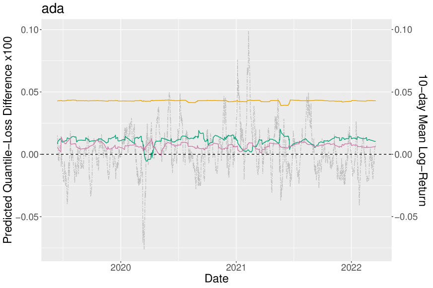
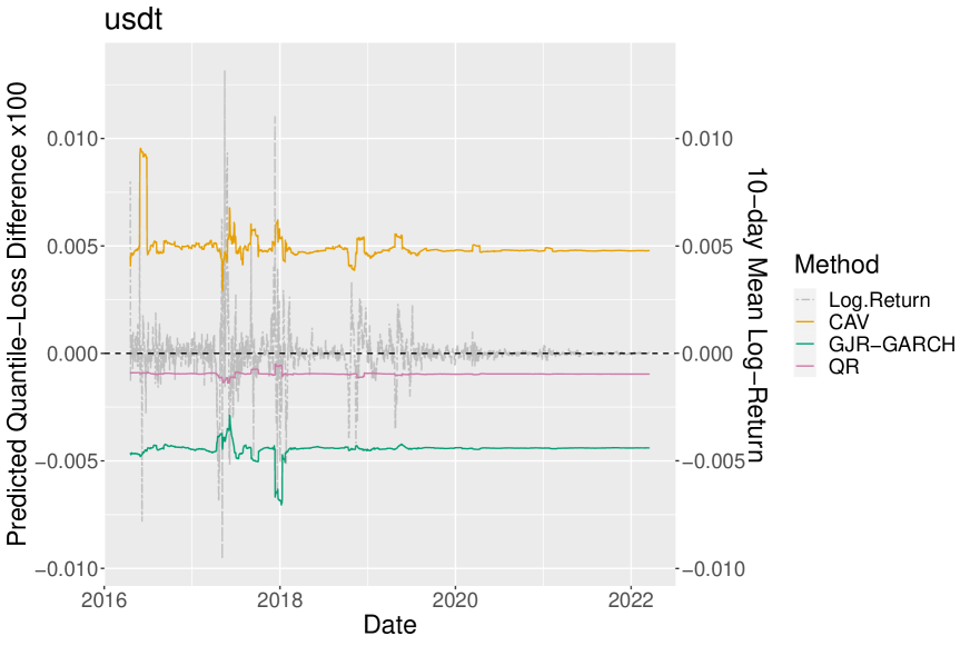
Figure 6: Rolling 30-day mean of predicted loss difference series of $h_{t}\hat{\beta}_{0}$ of CPA tests on Cardano/Tether (ada/usdt) predicted 5% VaR with $l=500$ for GRF vs. CAV (orange), GJR-GARCH (green), and QR (purple) with rolling mean 10-day log-returns in grey. A positive predicted loss difference indicates that the prediction error of GRF is smaller than of the compared method.

To further understand the drivers of the GRF performance, we obtain variable importance measures that depict the frequency of inclusion in splits of the forest. The variable importance of a covariate $x_{p}$ is measured as the proportion of splits on $x_{p}$ relative to all splits in a respective layer $l$ (over all trees in a trained forest), weighted by layer $l$. In Figure 7, the importance difference of certain covariates over time for the three currencies is clearly visible.

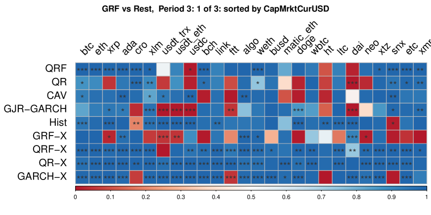
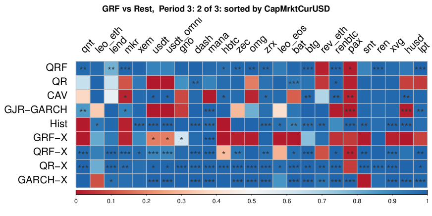
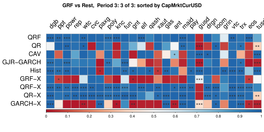
Figure 12: Overview of results for CPA-tests of GRF vs. all other methods for cryptocurrencies in the third period ordered by market cap from highest to lowest, left to right. The color of each box indicates the performance of GRF, with 1 indicating that GRF has a smaller predicted loss in 100% of cases. *, **, *** indicate significance on a level of 10%, 5%, and 1%.

Overall, the lagged return is very important for predicting VaR when returns are quite extreme relative to all returns in a specific asset, in the case of btc in times of hypes and crashes. Intuitively, this finding seems reasonable as in times of bubbles, when the volatility is driven by some short, bubble-like events and returns are highly variable, volatility lagged over a longer time horizon is less predictive for VaR and predictions are driven by events happening shortly before the prediction. In rather unstable times, but not in extreme cases, the lagged SD-measures gain importance, while the extra covariates only play a role for assets with relatively small volumes, e.g. when new currencies are created. This also explains why GRF-X performs much better for new, low-market-cap assets in Period 3 (see e.g. Figure 12 in the appendix).

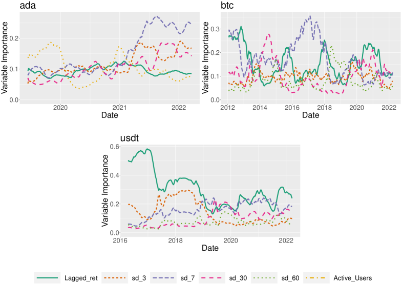
Figure 7: Rolling 30-day mean of the GRF variable importance in the out-of-sample period for the full data of ada, btc, and usdt, for predicted one-day ahead 5% VaR with $l=500$. Plotted are the 5 most important variables for each cryptocurrency. Variable importance of covariate $x_{p}$ is measured as the proportion of splits on $x_{p}$ relative to all splits in a respective layer $l$ (over all trees in a trained forest), weighted by layer $l$. Variable description can be seen in Section 2.

Starting with ada, we see that it is the only asset of the three where the number of active addresses plays an important role, where for the other two assets, the 60-day lagged standard deviation is more important. The importance of variables can be split into two periods. The period until the beginning of 2021 is largely dominated by measures that somehow account for trading activity (Active_Users,Total_Users/_USD100/_USD10, Transactions). For reasons of clarity, we only plot the most important one of these measures, Active_Users. The spike of the latter in importance at the beginning of 2021 is likely caused by the massive increase in price and market cap during that time, representing a period of hype with many actively trading users. For the rest of the time period, lagged SD, mostly 3-day lagged SD, followed by 30-day and 60-day SD, is dominating the predictions of GRF. This change of importance seems reasonable as the structure of the asset fundamentally changes with the price increasing tenfold and the volume increasing strongly at the same time.

For btc, we have much more data covering 10 years, which is why the important variables change frequently in different periods. Lagged return is naturally important in phases of extreme hype and crashes that are characterized by large positive and negative returns, e.g. in the very beginning (where the price was still quite low), at the end of 2013 (the first time btc had a price of USD 1000), at the end of 2017 (with a price over USD 19,000), and from mid 2020 to the mid 2021, where there were multiple hypes and crashes during the Covid-19 pandemic. Between these hype periods, the lagged SDs are most important. In 2014-2015 and from the end of 2019 to mid 2021 , 30-day SD is contributing most to the GRF-predictions, followed by 7-day SD in 2016-2018 and 60-day SD 20 from 2018 to the end of 2019. This changing scheme is interesting, as 30-day SD seems to be a good predictor especially in very unstable times (return-wise), while 7-day and 60-day SD are more important in relatively stable times.

Finally, the stablecoin usdt is an exception, being largely dominated by the lagged return. Given that by construction usdt is essentially bound to the US dollar, its dynamic properties also largely correspond to those of standard currencies. From mid 2019, the prices and returns are rather stable and the volume increases strongly, and the influence lagged 7-day SD increases slightly, while still being less important than lagged return. This is not surprising, as usdt is quite stable in comparison to btc and ada.

6 Conclusion

In this paper, we show that random forests can significantly improve the forecasting performance for VaR-predictions when tailored to conditional quantiles. In both simulations and analyzing return data of 105 of the largest cryptocurrencies, the proposed GRF-type random forest shows superior prediction performance. In particular, the adaptive non-linear form of GRF appears to capture time-variations of volatility and spike-behavior in cryptocurrency returns especially well in contrast to more conventional financial econometric methods. We further show that the GRF is better in assessing the tail risk of cryptocurrencies in times where volatility in returns is high which often coincides with increased speculation in the market. In such periods, standard time-series based procedures, even when augmented with external factors, are substantially inferior in VaR predictions suggesting that a comparison of predicted losses could serve as an easy, empirical pre-screening device to detect such speculative bubbles.

Our findings are highly relevant for the risk assessment of cryptocurrencies where we show that classic methods might lead to a miss-quantification of associated risks. Such results directly impact investment and hedging decisions for respective assets. Specifically, we detect superior performance of GRF especially for highly volatile cryptocurrencies that have a high number of active users and could thus be potentially prone to speculation and hypes. On the other hand, for the class of stablecoins that are usually tied to some large, classic currency such as the USD, and which are usually dominated by a smaller number of large accounts, other classic methods such as GJR-GARCH or quantile regression are more on par with GRF. This corresponds also to the simulation results mimicking the behavior of conventional assets such as as stock returns where the advantage of GRF decreases. Major gains of GRF, however, occur the more cryptocurrency-like the set-up becomes.

The proposed random forest methodology allows identifying important external factors despite the non-linearity of the methodology. We show that such factors are time-varying and changing particularly in unstable times. For future research, this set of covariates could even be further augmented with other potentially driving real-time factors, such as for example properly extracted and filtered social media information. The relevance of such factors might also provide additional guidance for relevant exogenous information to be included in standard parametric models such as CAViaR.

Appendix A Appendix

Table 10: Overview of Non-Stationarity Tests

	KPSS_level	KPSS_trend	ADF
algo	0.09	0.02	0.01
alpha	0.02	0.10	0.01
bnb	0.06	0.05	0.01
bnb_eth	0.06	0.05	0.01
btc	0.05	0.10	0.01
crv	0.10	0.03	0.01
dash	0.07	0.10	0.01
dcr	0.10	0.08	0.01
dot	0.10	0.10	0.01
eth	0.10	0.08	0.01
ftt	0.10	0.04	0.01
gno	0.10	0.10	0.01
gnt	0.10	0.04	0.01
icp	0.10	0.02	0.01
lend	0.10	0.02	0.01
loom	0.05	0.10	0.01
neo	0.10	0.08	0.01
omg	0.10	0.02	0.01
poly	0.04	0.10	0.01
ppt	0.10	0.07	0.01
snx	0.02	0.10	0.01
sushi	0.10	0.01	0.01
uni	0.10	0.08	0.01
weth	0.05	0.10	0.01
wtc	0.10	0.09	0.01
xem	0.07	0.10	0.01
xmr	0.10	0.04	0.01
xtz	0.10	0.09	0.01
yfi	0.08	0.10	0.01

Note: Values in columns show p-values for KPSS-test and ADF-tests as described in Section 2. We only show values for assets that have values smaller than $0.1$ for the KPSS-tests. No asset had p-values larger than $0.01$ for the ADF-tests.

Table 11: Overview of All Employed Crypto Assets

id	Asset	Start-Date	End-Date	Obs.	X	Time Periods	id	Asset	Start-Date	End-Date	Obs.	X	Time Periods
1inch	1inch	2020-12-26	2022-03-21	451	7		eos	EOS	2018-06-09	2022-03-21	1382	2	3
aave	Aave	2020-10-10	2022-03-21	528	7		eos_eth	EOS ETH	2017-06-29	2018-06-02	339	7
ada	Cardano	2017-12-01	2022-03-21	1572	7	3	etc	Ethereum Classic	2016-07-25	2022-03-21	2066	9	3
algo	Algorand	2019-06-22	2022-03-21	1004	7	3	eth	Ethereum	2015-08-08	2022-03-21	2418	9	2,3
alpha	Alpha Finance Lab	2020-10-11	2022-03-21	527	7		ftt	FTX Token	2019-08-20	2022-03-21	945	7	3
ant	Aragon	2017-08-29	2022-03-21	1666	7	3	fun	FunFair	2017-09-02	2022-03-21	1662	7	3
bal	Balancer	2020-06-25	2022-03-21	635	7		fxc	Flexacoin	2019-07-17	2021-01-25	559	6
bat	Basic Attention Token	2017-10-06	2022-03-21	1628	7	3	gas	Gas	2017-08-08	2022-03-21	1687	7	3
bch	Bitcoin Cash	2017-08-01	2022-03-21	1694	8	3	gno	Gnosis	2017-05-02	2022-03-21	1785	7	3
bnb	Binance Coin	2017-07-15	2019-04-22	647	7		gnt	Golem (gnt)	2017-02-19	2022-03-21	1857	7	3
bnb_eth	bnb_eth	2017-07-15	2019-04-22	647	7		grin	Grin	2019-01-29	2022-03-21	1148	2	3
bsv	Bitcoin SV	2018-11-15	2022-03-21	1220	8		gusd	Gemini Dollar	2018-09-16	2022-03-21	1283	7	3
btc	Bitcoin	2010-07-18	2022-03-21	4265	9	1,2,3	hbtc	Huobi Bitcoin	2019-12-09	2022-03-21	834	5	3
btg	Bitcoin Gold	2017-10-25	2022-03-21	1609	7	3	hedg	HedgeTrade	2019-11-02	2022-01-27	818	7
busd	Binance USD	2019-09-20	2022-03-21	914	7	3	ht	Huobi Token	2019-03-06	2022-03-21	1112	7	3
comp	Compound	2020-06-18	2022-03-21	642	7		husd	HUSD	2019-07-20	2022-03-21	976	7	3
cro	Crypto.com Coin	2019-03-20	2022-03-21	1098	7	3	icp	Internet Computer	2021-05-11	2022-03-21	315	7
crv	Curve DAO Token	2020-08-15	2022-03-21	584	7		kcs	KuCoin Token	2020-04-04	2022-03-22	718	0
cvc	Civic	2017-09-11	2022-03-21	1653	7	3	knc	Kyber Network	2017-09-27	2022-03-21	1637	7	3
dai	Dai	2019-11-20	2022-03-21	853	7	3	lend	Aave (lend)	2017-12-09	2022-03-21	1564	7	3
dash	Dash	2014-02-08	2022-03-21	2964	8	1,2,3	leo_eos	UNUS SED LEO EOS	2019-05-21	2022-03-21	1036	3	3
dcr	Decred	2016-05-17	2022-03-21	2133	8	2	leo_eth	UNUS SED LEO ETH	2019-05-21	2022-03-21	1036	7	3
dgb	DigiByte	2015-02-10	2022-03-21	2597	8	2,3	link	Chainlink	2017-09-29	2022-03-21	1635	7	3
doge	Dogecoin	2014-01-23	2022-03-21	2980	8	1,2,3	loom	Loom Network	2018-05-03	2022-03-21	1419	7	3
dot	Polkadot	2020-08-20	2022-03-21	579	7		lpt	Livepeer	2018-12-20	2022-03-21	1182	7	3
drgn	Dragonchain	2018-01-03	2022-03-21	1539	7	3	ltc	Litecoin	2013-04-01	2022-03-21	3277	8	1,2,3
elf	aelf	2017-12-22	2022-03-21	1551	7	3	maid	MaidSafeCoin	2014-07-10	2022-03-21	2812	7	2,3

Table 11: (Continued)

id	Asset	Start-Date	End-Date	Obs.	X	Time Periods	id	Asset	Start-Date	End-Date	Obs.	X	Time Periods
mana	Decentraland	2017-08-25	2022-03-21	1670	7	3	tusd	TrueUSD	2018-07-06	2022-03-21	1355	0	3
matic_eth	matic_eth	2019-04-27	2022-03-21	1060	7	3	uma	UMA	2020-09-08	2022-03-21	560	7
mkr	Maker	2017-12-26	2022-03-21	1547	7	3	uni	Uniswap	2020-09-18	2022-03-21	550	7
neo	Neo	2017-07-15	2022-03-21	1711	7	3	usdc	USD Coin	2018-09-28	2022-03-21	1271	7	3
nxm	Nexus Mutual	2020-08-26	2022-03-21	573	7		usdk	USDK	2020-06-13	2022-03-21	647	7
omg	OMG Network	2017-07-15	2022-03-21	1711	7	3	usdt	Tether	2014-10-06	2022-03-21	2724	7	2,3
pax	Paxos Standard	2018-11-30	2022-03-21	1208	7	3	usdt_eth	TetherETH	2017-11-28	2022-03-21	1575	7	3
paxg	PAX Gold	2020-02-15	2022-03-21	766	7	3	usdt_omni	usdt_omni	2014-10-06	2022-03-21	2724	7	2,3
pay	TenX	2017-10-03	2022-03-21	1631	7	3	usdt_trx	TetherTRON	2019-04-16	2022-03-21	1071	7	3
perp	Perpetual Protocol	2021-02-04	2022-03-21	411	7		vtc	Vertcoin	2014-01-29	2022-03-21	2974	8	1,2,3
poly	Polymath	2018-06-15	2022-03-21	1376	7	3	wbtc	Wrapped Bitcoin	2018-11-27	2022-03-21	1211	7	3
powr	Power Ledger	2017-11-02	2022-03-21	1601	7	3	weth	Wrapped Ether	2017-12-18	2022-03-21	1555	7	3
ppt	Populous	2017-09-20	2022-03-21	1644	7	3	wnxm	Wrapped NXM	2020-08-26	2022-03-21	573	7
qash	QASH	2017-11-06	2022-03-21	1597	7	3	wtc	Waltonchain	2017-08-28	2022-03-21	1667	7	3
qnt	Quant	2019-03-16	2022-03-21	1102	7	3	xaut	Tether Gold	2020-02-24	2022-03-21	757	7	3
ren	Ren	2018-12-07	2022-03-21	1201	7	3	xem	NEM	2015-04-01	2022-03-21	2547	2	2,3
renbtc	renBTC	2020-05-13	2022-03-21	678	7	3	xlm	Stellar	2015-09-30	2022-03-21	2365	7	2,3
rep	Augur	2016-10-04	2022-03-21	1995	7	3	xmr	Monero	2014-05-20	2022-03-21	2863	3	2,3
rev_eth	rev_eth	2020-03-26	2022-03-21	726	7	3	xrp	XRP	2014-08-15	2022-03-21	2776	7	2,3
sai	Sai	2017-12-23	2019-11-30	708	7		xtz	Tezos	2018-06-30	2022-03-21	1361	7	3
snt	Status	2017-06-20	2022-03-21	1736	7	3	xvg	Verge	2017-09-30	2022-03-21	1634	8	3
snx	Synthetix	2020-04-09	2022-03-21	712	7	3	yfi	yearn.finance	2020-07-25	2022-03-21	605	7
srm	Serum	2020-08-11	2022-03-21	588	7		zec	Zcash	2016-10-29	2022-03-21	1970	8	3
sushi	SushiSwap	2020-09-01	2022-03-21	567	7		zrx	0x	2017-08-11	2022-03-21	1684	7	3
swrv	Swerve	2020-09-22	2022-03-21	546	7
trx	TRON	2018-06-25	2022-03-21	1366	2	3
trx_eth	TronETH	2017-10-07	2018-06-25	262	7

Note: Obs. is the number of observations in total, i.e. including also the time points used for training. X depicts the number of additional covariates contained for each cryptocurrency, and Time Periods describes the sub-periods that the specific currency is in. Blank spaces indicate that a currency is not contained in any sub-period, which can occur when the currency is not available for the full out-of-sample sub-period.

Table 12: External Covariates and Descriptions

Variable Name	Coding Coinmetrics	Description
Active_Users	AdrActCnt	The number of unique active daily addresses
Total_Users	AdrBalCnt	The number of unique addresses that hold any amount of native units of that currency
Total_Users_USD100	AdrBalUSD100Cnt	The number of unique addresses that hold at least 100 USD of native units of that currency
Total_Users_USD10	AdrBalUSD10Cnt	The number of unique addresses that hold at least 10 USD of native units of that currency
SER	SER	The supply equality ratio, i.e. the ratio of supply held by addresses with less than 1 over 10 millionth of the current supply to the top one percent of addresses with the highest current supply
Transactions	TxCnt	The number of daily initiated transactions
Velocity	VelCur1yr	The velocity of supply in the current year, which describes the the ratio of current supply to the sum of the value transferred in the last year

Note: variable coding corresponds to https://docs.coinmetrics.io/. Detailed variable descriptions are available on https://docs.coinmetrics.io/info/metrics.

Table 13: Medians of P-Values for DQ-Tests Sorted by Covariate Values in Different Time Periods

Period	Sorting	GRF	QRF	QR	CAV	GJR-GARCH	Hist	GRF-X	QRF-X	QR-X	GARCH-X
High Group
SER
1	1 Highest	0.16	0.92	0.00	0.00	0.12	0.00	0.01	0.00	0.00	0.00
2	5 Highest	0.16	0.08	0.20	0.19	0.11	0.08	0.13	0.07	0.00	0.00
3	15 Highest	0.47	0.05	0.22	0.11	0.21	0.01	0.51	0.12	0.00	0.00
Number of Active Users
1	1 Highest	0.16	0.92	0.00	0.00	0.12	0.00	0.01	0.00	0.00	0.00
2	5 Highest	0.16	0.09	0.40	0.19	0.11	0.08	0.13	0.07	0.00	0.00
3	15 Highest	0.38	0.06	0.05	0.01	0.21	0.00	0.17	0.18	0.00	0.00
7-Day Lagged Standard Deviation
1	1 Highest	0.16	0.02	0.03	0.00	0.01	0.00	0.00	0.00	0.00	0.02
2	12 Highest	0.29	0.06	0.23	0.21	0.20	0.12	0.16	0.05	0.00	0.00
3	60 Highest	0.19	0.02	0.03	0.01	0.23	0.01	0.21	0.05	0.00	0.04
Low Group
SER
1	4 Lowest	0.13	0.28	0.10	0.10	0.02	0.00	0.00	0.00	0.00	0.00
2	10 Lowest	0.29	0.10	0.06	0.31	0.25	0.10	0.32	0.06	0.00	0.09
3	62 Lowest	0.07	0.04	0.03	0.02	0.32	0.00	0.18	0.07	0.00	0.06
Number of Active Users
1	4 Lowest	0.13	0.28	0.10	0.10	0.02	0.00	0.00	0.00	0.00	0.00
2	10 Lowest	0.42	0.09	0.06	0.31	0.20	0.10	0.26	0.06	0.00	0.09
3	62 Lowest	0.13	0.04	0.07	0.03	0.32	0.01	0.21	0.07	0.00	0.07
7-Day Lagged Standard Deviation
1	4 Lowest	0.13	0.42	0.10	0.10	0.07	0.00	0.01	0.00	0.00	0.00
2	3 Lowest	0.00	0.11	0.00	0.32	0.00	0.00	0.00	0.06	0.00	0.00
3	17 Lowest	0.06	0.47	0.24	0.30	0.60	0.00	0.15	0.45	0.00	0.00

Note: The currencies are divided into two groups based on specific covariate values for each time period. The groups are constructed to best separate the sorted covariate values of the currencies. They are therefore separated at their steepest decay to obtain two groups with homogeneous covariate values. Detailed plots for the cutoff can be found in Figure 10. The remaining details correspond to Table 6.

Table 14: Performance and Significance of CPA-tests with GRF-X Over Different Time Periods

GRF-X vs.:	GRF	QRF	QR	CAV	GJR-GARCH	Hist	QRF-X	QR-X	GARCH-X
Share of GRF With Better Performance
Period 1	0.40	1.00	0.80	0.60	0.80	1.00	1.00	1.00	1.00
Period 2	0.60	1.00	0.67	0.87	0.80	1.00	1.00	1.00	1.00
Period 3	0.55	0.90	0.66	0.75	0.66	0.90	0.94	0.96	0.73
Full Data	0.54	0.89	0.72	0.76	0.73	0.83	0.92	0.97	0.76
Share of GRF With Significantly Better Performance
Period 1	0.00	0.20	0.20	0.00	0.20	1.00	1.00	1.00	0.60
Period 2	0.20	0.40	0.27	0.20	0.40	0.80	0.93	0.93	0.67
Period 3	0.12	0.40	0.19	0.23	0.19	0.58	0.73	0.81	0.51
Full Data	0.13	0.39	0.30	0.24	0.19	0.47	0.69	0.86	0.52

The top part shows summary values that are shares over all cryptocurrencies in the respective time period. It describes the number of times that GRF-X had a better performance (i.e. more than 50% of predicted losses by the CPA test were smaller for the GRF-X) relative to all crytpocurrencies (in that period), and the number of times that GRF-X was significantly better (at least at a 10% level) as judged by the CPA test over all crytpocurrencies (in that period). The bottom part shows the detailed results of CPA-tests with the color of each box indicating the performance of GRF-X. Blue signifies a performance of 1, meaning that GRF-X has a smaller predicted loss in 100% of cases. *, **, *** shows significance on a level of 10%, 5%, and 1%. The values are ordered by 30 day lagged standard deviation from highest to lowest.

Table 15: Difference Between Covariates of Cryptos Where GRF-X is Better vs. Worse

	Period 1	Period 2	Period 3	Full Data
Ret	1.20	0.63	-0.40	-0.08
Active_Users	0.34	0.22	0.32	0.39
Total_Users	0.79	0.26	0.31	0.34
Total_Users_USD100	0.22	0.23	0.22	0.27
Total_Users_USD10	0.41	0.23	0.16	0.20
CapMrktCurUSD	0.08	0.16	0.45	0.38
SER	1.07	0.72	0.17	0.22
Transactions	0.42	0.06	3.26	3.74
Velocity	4.68	4.44	1.31	1.23
sd_3	0.89	0.31	0.65	0.65
sd_7	0.91	0.32	0.64	0.64
sd_30	0.90	0.33	0.63	0.64
sd_60	0.91	0.34	0.63	0.65

Note: values are shares of groups of cryptocurrencies where at least two of CAV, QR, and GJR-GARCH have better CPA-performance than GRF-X divided by the remaining rest. Raw values before division are mean values over all cryptocurrencies for the median of each covariate in the respective time period.

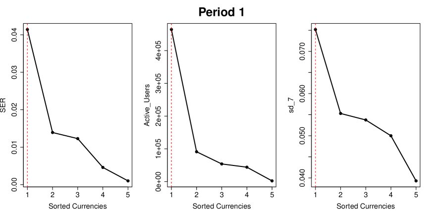
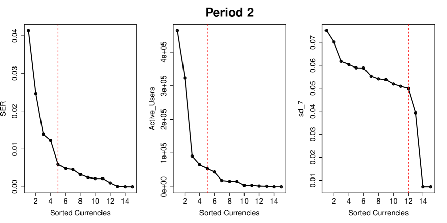
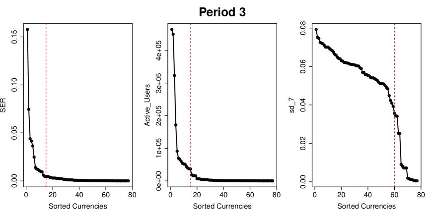
Figure 10: Sorted variable means and cutoff values for groups that separate the cryptocurrencies based on variables for each period. These groups are used in backtests in Table 13. The cutoff value is depicted in red dotted lines fro each variable and time period.

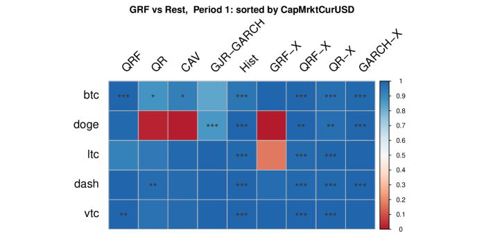
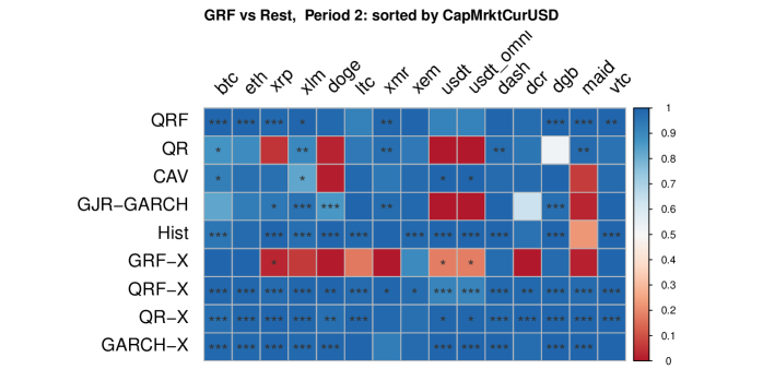
Figure 11: Overview of results for CPA-tests of GRF vs. all other methods for cryptocurrencies in the first and second period ordered by market cap from highest to lowest. The color of each box indicates the performance of GRF, with 1 indicating that GRF has a smaller predicted loss in 100% of cases. *, **, *** indicate significance on a level of 10%, 5%, and 1%.

Figure 14: Log-returns of the specific cryptocurrencies analyzed in Substection 5.2.

Table 16: Simulation: $1\%$ VaR

Rolling Window	$l=500$				$l=1000$
	DQ	Kupiec	Christoffersen	AoE		DQ	Kupiec	Christoffersen	AoE
Sim GARCH Normal
QRF	$0.995$ $(0.002)$	$0.910$ $(0.017)$	$0.855$ $(0.029)$	1.894		$0.830$ $(0.053)$	$0.580$ $(0.128)$	$0.395$ $(0.180)$	1.751
GRF	$0.635$ $(0.121)$	$0.120$ $(0.396)$	$0.115$ $(0.388)$	1.265		$0.410$ $(0.318)$	$0.100$ $(0.459)$	$0.050$ $(0.518)$	1.193
QR	$0.945$ $(0.018)$	$0.500$ $(0.122)$	$0.485$ $(0.155)$	1.575		$0.520$ $(0.235)$	$0.140$ $(0.433)$	$0.090$ $(0.469)$	1.273
Hist	$0.830$ $(0.046)$	$0.045$ $(0.421)$	$0.195$ $(0.339)$	1.231		$0.675$ $(0.171)$	$0.120$ $(0.477)$	$0.140$ $(0.456)$	1.122
NormFit	$0.700$ $(0.116)$	$0.055$ $(0.470)$	$0.200$ $(0.392)$	1.165		$0.625$ $(0.209)$	$0.130$ $(0.441)$	$0.145$ $(0.450)$	1.152
CAV	$0.890$ $(0.038)$	$0.365$ $(0.181)$	$0.340$ $(0.215)$	1.486		$0.450$ $(0.304)$	$0.130$ $(0.435)$	$0.080$ $(0.508)$	1.245
GARCH(1,1)	$0.440$ $(0.268)$	$0.060$ $(0.468)$	$0.150$ $(0.412)$	1.128		$0.310$ $(0.408)$	$0.060$ $(0.532)$	$0.075$ $(0.525)$	1.072
Sim GARCH t
QRF	$0.990$ $(0.002)$	$0.890$ $(0.016)$	$0.845$ $(0.029)$	1.942		$0.815$ $(0.060)$	$0.665$ $(0.108)$	$0.500$ $(0.152)$	1.801
GRF	$0.625$ $(0.127)$	$0.135$ $(0.372)$	$0.155$ $(0.396)$	1.286		$0.410$ $(0.297)$	$0.100$ $(0.455)$	$0.055$ $(0.523)$	1.222
QR	$0.925$ $(0.014)$	$0.570$ $(0.106)$	$0.575$ $(0.134)$	1.676		$0.565$ $(0.227)$	$0.165$ $(0.393)$	$0.130$ $(0.431)$	1.290
Hist	$0.755$ $(0.077)$	$0.080$ $(0.412)$	$0.215$ $(0.385)$	1.232		$0.665$ $(0.160)$	$0.125$ $(0.454)$	$0.175$ $(0.434)$	1.133
NormFit	$0.890$ $(0.028)$	$0.655$ $(0.092)$	$0.670$ $(0.096)$	1.693		$0.760$ $(0.083)$	$0.510$ $(0.184)$	$0.450$ $(0.209)$	1.669
CAV	$0.815$ $(0.042)$	$0.320$ $(0.190)$	$0.310$ $(0.230)$	1.466		$0.425$ $(0.298)$	$0.155$ $(0.410)$	$0.090$ $(0.472)$	1.248
GARCH(1,1)	$0.855$ $(0.045)$	$0.750$ $(0.057)$	$0.745$ $(0.068)$	1.769		$0.595$ $(0.174)$	$0.500$ $(0.176)$	$0.430$ $(0.196)$	1.680
Sim SAV-Model
QRF	$0.990$ $(0.001)$	$0.940$ $(0.015)$	$0.835$ $(0.028)$	1.891		$0.810$ $(0.063)$	$0.575$ $(0.133)$	$0.405$ $(0.187)$	1.749
GRF	$0.585$ $(0.140)$	$0.065$ $(0.417)$	$0.045$ $(0.462)$	1.251		$0.300$ $(0.352)$	$0.080$ $(0.460)$	$0.035$ $(0.550)$	1.180
QR	$0.940$ $(0.015)$	$0.445$ $(0.129)$	$0.375$ $(0.179)$	1.553		$0.560$ $(0.200)$	$0.190$ $(0.406)$	$0.090$ $(0.473)$	1.289
Hist	$0.360$ $(0.239)$	$0.060$ $(0.515)$	$0.075$ $(0.534)$	1.195		$0.275$ $(0.415)$	$0.060$ $(0.513)$	$0.060$ $(0.597)$	1.097
NormFit	$0.215$ $(0.449)$	$0.105$ $(0.452)$	$0.110$ $(0.527)$	1.166		$0.240$ $(0.520)$	$0.135$ $(0.448)$	$0.090$ $(0.553)$	1.147
CAV	$0.855$ $(0.035)$	$0.255$ $(0.207)$	$0.250$ $(0.239)$	1.444		$0.485$ $(0.273)$	$0.075$ $(0.439)$	$0.050$ $(0.518)$	1.221
GARCH(1,1)	$0.215$ $(0.407)$	$0.090$ $(0.502)$	$0.090$ $(0.532)$	1.155		$0.210$ $(0.513)$	$0.105$ $(0.471)$	$0.055$ $(0.574)$	1.122
Sim GARCH Bitcoin fit
QRF	$0.975$ $(0.004)$	$0.910$ $(0.017)$	$0.855$ $(0.029)$	1.894		$0.750$ $(0.090)$	$0.580$ $(0.128)$	$0.395$ $(0.180)$	1.751
GRF	$0.470$ $(0.207)$	$0.120$ $(0.396)$	$0.115$ $(0.388)$	1.265		$0.275$ $(0.424)$	$0.100$ $(0.459)$	$0.050$ $(0.518)$	1.193
QR	$0.880$ $(0.040)$	$0.500$ $(0.122)$	$0.485$ $(0.155)$	1.575		$0.370$ $(0.328)$	$0.140$ $(0.433)$	$0.090$ $(0.469)$	1.273
Hist	$0.675$ $(0.090)$	$0.045$ $(0.421)$	$0.195$ $(0.339)$	1.231		$0.530$ $(0.259)$	$0.120$ $(0.477)$	$0.140$ $(0.456)$	1.122
NormFit	$0.540$ $(0.203)$	$0.055$ $(0.470)$	$0.200$ $(0.392)$	1.165		$0.500$ $(0.296)$	$0.130$ $(0.441)$	$0.145$ $(0.450)$	1.152
CAV	$0.745$ $(0.091)$	$0.105$ $(0.405)$	$0.155$ $(0.400)$	1.243		$0.435$ $(0.345)$	$0.045$ $(0.486)$	$0.030$ $(0.555)$	1.046
GARCH(1,1)	$0.345$ $(0.328)$	$0.065$ $(0.459)$	$0.190$ $(0.385)$	1.157		$0.215$ $(0.510)$	$0.050$ $(0.537)$	$0.070$ $(0.512)$	1.082

Results for $1\%$ VaR show rejection rates of t-tests of empirical levels against the nominal level of $1\%$ for DQ-, Kupiec- and Christoffersen-tests and mean p-values in parentheses. Higher p-values and lower rejection rates indicate better model performance. GARCH depicts an oracle GARCH-model that fits an GARCH(1,1) process with normally distributed errors.

References

- Ardia et al. (2019) Ardia, D., K. Boudt, and L. Catania (2019): “Generalized autoregressive score models in R: The GAS package,” Journal of Statistical Software, 88.
- Athey et al. (2019) Athey, S., J. Tibshirani, and S. Wager (2019): “Generalized random forests,” Annals of Statistics, 47, 1179–1203.
- Baur et al. (2018) Baur, D. G., K. H. Hong, and A. D. Lee (2018): “Bitcoin: Medium of exchange or speculative assets?” Journal of International Financial Markets, Institutions and Money, 54, 177–189.
- Bollerslev (1986) Bollerslev, T. (1986): “Generalized autoregressive conditional heteroskedasticity,” Journal of Econometrics, 31, 307–327.
- Breiman (1996) Breiman, L. (1996): “Some properties of splitting criteria,” Machine Learning, 24, 41–47.
- Breiman (2001) ——— (2001): “Random Forests,” Machine Learning, 45, 5–32.
- Breiman et al. (1984) Breiman, L., J. Friedman, C. J. Stone, and R. A. Olshen (1984): Classification and regression trees, CRC press.
- Cheah and Fry (2015) Cheah, E. T. and J. Fry (2015): “Speculative bubbles in Bitcoin markets? An empirical investigation into the fundamental value of Bitcoin,” Economics Letters, 130, 32–36.
- Christoffersen (1998) Christoffersen, P. F. (1998): “Evaluating Interval Forecasts,” International Economic Review, 39, 841.
- Chu et al. (2017) Chu, J., S. Chan, S. Nadarajah, and J. Osterrieder (2017): “GARCH Modelling of Cryptocurrencies,” Journal of Risk and Financial Management, 10, 17.
- Elendner et al. (2017) Elendner, H., S. Trimborn, B. Ong, and T. M. Lee (2017): “The Cross-Section of Crypto-Currencies as Financial Assets: Investing in Crypto-Currencies Beyond Bitcoin,” in Handbook of Blockchain, Digital Finance, and Inclusion, Volume 1: Cryptocurrency, FinTech, InsurTech, and Regulation, Elsevier, 145–173.
- Engle and Manganelli (2004) Engle, R. F. and S. Manganelli (2004): “CAViaR: Conditional autoregressive value at risk by regression quantiles,” Journal of Business and Economic Statistics, 22, 367–381.
- Ghysels and Nguyen (2019) Ghysels, E. and G. Nguyen (2019): “Price Discovery of a Speculative Asset: Evidence from a Bitcoin Exchange,” Journal of Risk and Financial Management, 12, 164.
- Giacomini and Komunjer (2005) Giacomini, R. and I. Komunjer (2005): “Evaluation and combination of conditional quantile forecasts,” Journal of Business and Economic Statistics, 23, 416–431.
- Giacomini and White (2006) Giacomini, R. and H. White (2006): “Tests of conditional predictive ability,” Econometrica, 74, 1545–1578.
- Gkillas and Katsiampa (2018) Gkillas, K. and P. Katsiampa (2018): “An application of extreme value theory to cryptocurrencies,” Economics Letters, 164, 109–111.
- Glaser et al. (2014) Glaser, F., K. Zimmermann, M. Haferkorn, M. C. Weber, and M. Siering (2014): “Bitcoin - Asset or currency? Revealing users’ hidden intentions,” ECIS 2014 Proceedings - 22nd European Conference on Information Systems, 1–14.
- Glosten et al. (1993) Glosten, L. R., R. Jagannathan, and D. E. Runkle (1993): “On the Relation between the Expected Value and the Volatility of the Nominal Excess Return on Stocks,” The Journal of Finance, 48, 1779–1801.
- Hafner (2020) Hafner, C. M. (2020): “Testing for Bubbles in Cryptocurrencies with Time-Varying Volatility,” Journal of Financial Econometrics, 18, 233–249.
- Hastie et al. (2009) Hastie, T., R. Tibshirani, and J. Friedman (2009): The Elements of Statistical Learning, Springer, second ed.
- Hencic and Gouriéroux (2015) Hencic, A. and C. Gouriéroux (2015): “Noncausal autoregressive model in application to bitcoin/USD exchange rates,” in Studies in Computational Intelligence, Springer, vol. 583, 17–40.
- Koenker and Bassett (1978) Koenker, R. and G. Bassett (1978): “Regression Quantiles,” Econometrica, 46, 33.
- Koenker and Hallock (2001) Koenker, R. and K. F. Hallock (2001): “Quantile regression,” Journal of economic perspectives, 15, 143–156.
- Kupiec (1995) Kupiec, P. H. (1995): “Techniques for Verifying the Accuracy of Risk Measurement Models,” The Journal of Derivatives, 3, 73–84.
- Kwiatkowski et al. (1992) Kwiatkowski, D., P. C. Phillips, P. Schmidt, and Y. Shin (1992): “Testing the null hypothesis of stationarity against the alternative of a unit root. How sure are we that economic time series have a unit root?” Journal of Econometrics, 54, 159–178.
- Liu et al. (2020) Liu, W., A. Semeyutin, C. K. M. Lau, and G. Gozgor (2020): “Forecasting Value-at-Risk of Cryptocurrencies with RiskMetrics type models,” Research in International Business and Finance, 54, 101259.
- Liu and Tsyvinski (2020) Liu, Y. and A. Tsyvinski (2020): “Risks and Returns of Cryptocurrency,” The Review of Financial Studies, 34, 2689–2727.
- Maciel (2020) Maciel, L. (2020): “Cryptocurrencies value-at-risk and expected shortfall: Do regime-switching volatility models improve forecasting?” International Journal of Finance & Economics.
- Meinshausen (2006) Meinshausen, N. (2006): “Quantile Regression Forests,” Journal of Machine Learning Research, 7, 983–999.
- Pafka and Kondor (2001) Pafka, S. and I. Kondor (2001): “Evaluating the RiskMetrics methodology in measuring volatility and Value-at-Risk in financial markets,” Physica A: Statistical Mechanics and its Applications, 299, 305–310.
- Petukhina et al. (2021) Petukhina, A., S. Trimborn, W. K. Härdle, and H. Elendner (2021): “Investing with cryptocurrencies – evaluating their potential for portfolio allocation strategies,” Quantitative Finance, 0, 1–29.
- Platanakis and Urquhart (2019) Platanakis, E. and A. Urquhart (2019): “Portfolio management with cryptocurrencies: The role of estimation risk,” Economics Letters, 177, 76–80.
- Selmi et al. (2018) Selmi, R., A. Tiwari, and S. Hammoudeh (2018): “Efficiency or speculation? A dynamic analysis of the Bitcoin market,” Economics Bulletin, 38, 2037–2046.
- Takeda and Sugiyama (2008) Takeda, A. and M. Sugiyama (2008): “N-Support Vector Machine As Conditional Value-At-Risk Minimization,” Proceedings of the 25th International Conference on Machine Learning, 1056–1063.
- Trimborn et al. (2020) Trimborn, S., M. Li, and W. K. Härdle (2020): “Investing with Cryptocurrencies - A Liquidity Constrained Investment Approach,” Journal of Financial Econometrics, 18, 280–306.
- Trucios et al. (2020) Trucios, C., A. K. Tiwari, and F. Alqahtani (2020): “Value-at-risk and expected shortfall in cryptocurrencies’ portfolio: A vine copula–based approach,” Applied Economics, 52, 2580–2593.
- Vigliotti and Jones (2020) Vigliotti, M. G. and H. Jones (2020): “The Rise and Rise of Cryptocurrencies,” in The Executive Guide to Blockchain, Springer, 71–91.