L-band Integral Field Spectroscopy of the HR 8799 Planetary System

Abstract

Understanding the physical processes sculpting the appearance of young gas-giant planets is complicated by degeneracies confounding effective temperature, surface gravity, cloudiness, and chemistry. To enable more detailed studies, spectroscopic observations covering a wide range of wavelengths is required. Here we present the first L-band spectroscopic observations of HR 8799 d and e and the first low-resolution wide bandwidth L-band spectroscopic measurements of HR 8799 c. These measurements were facilitated by an upgraded LMIRCam/ALES instrument at the LBT, together with a new apodizing phase plate coronagraph. Our data are generally consistent with previous photometric observations covering similar wavelengths, yet there exists some tension with narrowband photometry for HR 8799 c. With the addition of our spectra, each of the three innermost observed planets in the HR 8799 system have had their spectral energy distributions measured with integral field spectroscopy covering $\sim 0.9$ to $4.1~{}\mu\mathrm{m}$. We combine these spectra with measurements from the literature and fit synthetic model atmospheres. We demonstrate that the bolometric luminosity of the planets is not sensitive to the choice of model atmosphere used to interpolate between measurements and extrapolate beyond them. Combining luminosity with age and mass constraints, we show that the predictions of evolutionary models are narrowly peaked for effective temperature, surface gravity, and planetary radius. By holding these parameters at their predicted values, we show that more flexible cloud models can provide good fits to the data while being consistent with the expectations of evolutionary models.

1 Introduction

More than a decade of direct imaging photometric and spectroscopic probes of gas-giant exoplanets have provided an important understanding of the physical processes sculpting their atmospheres. The HR 8799 system, which includes four giant planets (Marois et al., 2010), is by far the most well studied system for direct imaging. In addition to the appeal of comparing the appearance of multiple coeval planets, HR 8799 is also observable from both hemispheres, includes a bright host star required for high-performance adaptive optics (AO) systems, and the planets are observed with projected separations and contrasts amenable for modern AO instruments at the world’s largest telescopes. In fact, the outermost planet falls outside the narrow field of view of many of the latest high angular resolution instruments.

Early studies identified that the HR 8799 planets occupied a rarefied locus of near-IR color magnitude diagrams (Marois et al., 2008), being redder and/or fainter than typical brown dwarfs with similar effective temperatures. Model atmosphere fits to the HR 8799 planets, and to other young directly imaged planetary mass companions, match these measurements reasonably well (Patience et al., 2010) but with scaling factors that implied planet radii ($<1~{}R_{\mathrm{Jup}}$) which are much too small to be consistent with our understanding of gas-giant planetary structure.

Atmospheric modelers and brown dwarf observers quickly aided our understanding of some of these observations by pointing out that atmospheres, especially substellar atmospheres, are not single parameter systems described only by effective temperature. Surface gravity, particularly for young planets that are low mass with extended radii, is an essential consideration for a proper interpretation of the data (see Stephens et al., 2009; Barman et al., 2011; Marley et al., 2012). Low gravity atmospheres can loft clouds above their photospheres at cooler temperatures than higher gravity objects (Barman et al., 2011; Marley et al., 2012). Additionally, low-gravity atmospheres are more susceptible to vigorous mixing that can alter the balance of chemical species in the photosphere, including the relative abundance of methane and carbon monoxide (Hubeny & Burrows, 2007).

Even so, model fits to data are plagued by degeneracies between temperature, gravity, cloudiness, and chemistry (see Currie et al., 2014). Cloud structure in particular is confounding because of the complex physics governing cloud formation (and dissipation) and because of the number of parameters needed to describe them, including cloud thickness, cloud coverage (patchy/homogeneous), cloud particle size distribution, and cloud composition, among others. For the HR 8799 planets in particular, models with either homogeneous cloud coverage and small grain size (e.g., Bonnefoy et al., 2016; Konopacky et al., 2013; Greenbaum et al., 2018) or patchy cloud models (e.g., Currie et al., 2011; Skemer et al., 2014; Currie et al., 2014) can provide reasonable fits to the data.

Detailed narrowband spectroscopic observations can enable studies to characterize certain aspects of planetary atmospheres in ways that do not seem to depend on the details of cloud structure, such as C/O ratio (Konopacky et al., 2013; Barman et al., 2015; Wang et al., 2020; Mollière et al., 2020). Photometric studies constraining a large portion of the planetary spectral energy distribution (SED) can be successful in breaking model degeneracies to constrain planet composition (Skemer et al., 2016). Notably, Wang et al. (2020) find that their free retrieval with L- and M-band data yields solutions that are closer to physically and chemically motivated models compared to excluding this wavelength range, and remark that this data data helps constrain the abundances and cloud condition. The Arizona Lenslets for Exoplanet Spectroscopy (ALES, Skemer et al., 2015, 2018a) instrument was built to increase the wavelength coverage of high-contrast spectroscopic observations to improve our understanding of gas-giant atmospheres.

In this paper, we present the first L-band spectroscopy of HR 8799 d, and e. For HR 8799 c some previous spectroscopic observations exist at these wavelengths, including the early work of Janson et al. (2010) presenting three spectral channels covering a small range of the atmospheric window, and the high-resolution work presented by Wang et al. (2018). We present the first broadband low-resolution spectroscopy of HR 8799 c in the L-band.

After describing our observations and data reduction approach in Section 2, we compare our measurements to those from the literature in Section 2.6 finding general agreement with earlier photometric measurements, although we identify some tension at LNB5 and LNB6 for HR 8799 c. With the addition of our data, each of the three innermost directly imaged planets in the HR 8799 system have had their emission spectra measured with low-resolution integral field spectrograph (IFS) spectroscopy spanning $\sim 0.9-4.1~{}\mu\mathrm{m}$. In Section 3 we compile data from the literature for each planet and describe a model fitting approach to match spectra from two families of synthetic atmosphere models and blackbodies. The results of our fitting are presented in Section 3.3. Our initial fitting approach did not impose any restrictions on planet radius or other bulk quantities. We show that the Barman/Brock family of models (Barman et al., 2011; Brock et al., 2021) are capable of providing reasonable fits to the data as well as reasonable planet radii in some cases, but that the radii required for the DRIFT-Phoenix models (Witte et al., 2011) were not consistent with expectations based on evolutionary models of gas-giant structure. As expected, the blackbody models provided neither a good approximation to the data nor reasonable radii.

Many previous studies have appealed to evolutionary models to constrain their atmospheric modeling efforts (e.g., Barman et al., 2011; Marley et al., 2012; Konopacky et al., 2013; Rajan et al., 2017; Brock et al., 2021). In Section 4 we develop a Monte Carlo approach to generating quantitative priors for atmospheric model fitting. This approach incorporates the details of constraints on system parameters such as age, mass, and luminosity, and results in priors for $T_{\mathrm{eff}}$, $\log(g)$, and radius that can be directly tied to specific evolutionary models.

For the HR 8799 planets, we point out that the luminosity of each, with such broad spectroscopic coverage, is tightly constrained —depending little on the choice of well-scaled atmospheric model used to interpolate between observations and extrapolate beyond them. We use this luminosity together with constraints on system age and planet masses, to show that the predictions of hot-start luminosity models are narrowly peaked in effective temperature, surface gravity, and radius. We follow the example of Brock et al. (2021) and rerun our fits, fixing effective temperature, surface gravity and radius, and using more flexible atmospheric models to explore what can be inferred about cloud structure assuming gas-giant evolution models are reliable. Finally, in Section 5 we summarize our results and comment on future applications of both the technology demonstrated and the analysis performed particularly towards Gaia-detected companions.

2 Observations and data reduction

We observed HR 8799 on 2019 September 18 for 1 hour 53 minutes with the upgraded LBTI/ALES instrument (Skemer et al., 2018a; Hinz et al., 2018). ALES is an adaptive optics-fed integral field spectrograph with sensitivity out to 5 microns (Skemer et al., 2015, 2018a) and is used as a mode of the LMIRCam instrument (Skrutskie et al., 2010; Leisenring et al., 2012), part of the Large Binocular Telescope Interferometer architecture (Hinz et al., 2016). We used the main mode of ALES with a square field of view of $\sim$2.2 arcseconds on a side with a spectral resolution of $\sim$35, spanning the $2.8-4.2$ $\mu$m range. The detector integration time was set to 3.934 seconds and the first and last 0.492-second read of each ramp was saved to enable the subtraction of detector reset noise (correlated double sampling). The conditions were stable with seeing between 0.8 and 1.1 arcseconds. We acquired 1300 frames on-target for a total of 1 hour 24 minutes. The LBTI architecture does not include an instrument derotator and our images include a total field rotation of $85\fdg 64$ through meridian crossing.

The observations were conducted as part of early characterization efforts using a new apodizing phase plate upstream of the IFS within LMIRCam. The double-grating 360^∘ vector apodizing phase plate (dgvAPP360 Doelman et al., 2020; Wagner et al., 2020) suppresses the stellar diffraction halo by multiple orders of magnitude over the full $2-5~{}\mu\mathrm{m}$ bandwidth. The dgvAPP360 is different from the more commonly used grating-vAPP (Snik et al., 2012; Otten et al., 2017; Doelman et al., 2021), which creates two images of the star each with a D-shaped dark zones on opposite sides. The additional grating in the dgvAPP360 diffracts the light back on-axis, such that the two apodized images overlap, resulting in a single image of the star. Furthermore, the phase design of the dgvAPP360 creates a dark zone in a full annulus (covering 360^∘) surrounding the star. The resulting point spread function (PSF) is much smaller compared to the gvAPP and is consequently better suited for the small field of view of an IFS.

As a pupil plane optic, the dgvAPP360 is particularly well suited for ALES, as careful alignment of the IFS magnifiers with a focal plane spot is not necessary. Since the dgvAPP360 response is tip/tilt invariant, drifts in the PSF location during observing do not result in a loss of performance, i.e. dark zone contrast. Additionally, the location of the star is known in every frame. This is ideal because with our short thermal-IR exposure times we are able to increase contrast with post-processing shift and add techniques.

In order to increase on-source efficiency we chose not to periodically nod to a sky position to track variable background emission. Instead, we collected a total of 99 background frames, where the first 13 were taken after 100 science frames and the other 86 directly after the science sequence. We achieved a ratio of on-target to background integration of 93%. However, as described in Section 2.3, our original plan for removing the sky background at each wavelength within each cube was complicated as a result of an instrument related issue, requiring a more sophisticated data reduction approach than envisioned at the time our observations were designed. This issue is the movement of the stellar PSF and associated structures with respect to non-uniform thermal background.

Wavelength calibration of our spectral cubes was achieved by observing through four narrowband ($R\sim 100$) filters. The filters, spanning $2.9~{}\mu\mathrm{m}$ to $3.9~{}\mu\mathrm{m}$, are all located upstream of the ALES optics within LMIRCam, and are observed sequentially (Stone et al., 2018). Thermal emission from the sky fills the ALES field of view and provides fiducial wavelength spots at every position. Images were saved with 3.934 second exposures. For the two shorter wavelength filters we saved 25 frames each. For the two longer wavelength filters we saved 10 frames each. We saved 200 dark frames with the same exposure time.

2.1 Raw Frame Preprocessing

Prior to making cubes, each of our ALES frames were preprocessed to correct for reset noise, variable channel offsets, hot pixels, and a fixed light leak from within the instrument that causes off-axis light to pass through the lenslet array and fill some of the pixels between the on-sky spectral traces. This light leak can bias the measured position of the wavelength calibration spots and result in an inaccurate estimate of some of the spectral spatial profiles, significantly affecting the quality of our spectral cubes.

For each image we subtracted the first read from the last. This removes the reset noise and most of the channel offsets seen in the raw images. Residual channel offsets were then removed using a median of the $4\times 64$ lower overscan pixels in each channel. We noticed that the 127th and 128th columns (and the corresponding columns every 128 pixels) behaved differently than the other columns within their channels, so we treated these individually, subtracting only the median of the lower four overscan pixels in the same column. In the orthogonal direction, eight overscan pixels in each row are median combined and the resulting 2048 pixel column is then smoothed with a Savitzky-Golay filter using a window length of 31 and polynomial order of 3. The resulting smoothed overscan column is then removed from each column in the image.

Figure 1: Flowchart of the data-reduction method.

To correct for the light leak, an empirical model of the leak was subtracted from each frame. To build this model, we first median combined the narrowband filter wavelength calibration images for each of the four filters. The resulting medians were then median combined. This approach removes the narrow spots, leaving behind only the light leak signal.

Bad pixels in each processed frame were replaced using the median of the 4 nearest good pixels. Bad pixels were identified as overly hot in dark frames and/or overly cold in flat illuminated frames.

2.2 Spectral cube extraction

We extracted $(x,y,\lambda)$ data cubes using an inverse variance and spatial profile weighted extraction approach on each of the $63\times 67$ micro-spectra across the ALES field (Horne, 1986; Briesemeister et al., 2018). To build extraction weights we used the 99 sky images to define the spatial profile and variance. We built the spatial profile for each microspectrum assuming a constant profile with wavelength and median combining along wavelength direction. To mitigate crosstalk we enforced a seven pixel wide window, which accommodates the full width at half maximum for spectra near the center of the field of view, but crops more light for some aberrated spectra near the edge of the field of view. For each of the microspectra we also masked out the right side of the spatial profile for the bluest wavelengths of the spectrum where the risk of contamination (spectral crosstalk) from the brightest red part of the neighboring microspectrum is highest.

A quadratic wavelength solution, mapping pixel position to wavelength, was fit to each spectrum using the peak pixel for each narrowband wavelength filter image and the corresponding wavelength from a cryogenic filter trace. Since each of the microspectra are not sampled in exactly the same way by the pixels of LMIRCam, in order to produce a spectral cube with constant wavelength at each slice, cubic interpolation was used on each spectrum to extract the same wavelengths at each position.

The new ALES lenslet array has lower amplitude optical aberrations than the previous array, but the spot produced by each lenslet is affected by a residual astigmatism whose axis rotates as a function of position in the array. This creates a varying spatial profile and a varying spectral resolution that both contribute to a varying throughput as a function of position and wavelength. A lenslet flat was generated to quantify this throughput by extracting a cube of the median sky image and normalizing each wavelength slice. This flat is then used to correct each of the science cubes.

As a final step, we binned the data per four frames in time by averaging, reducing the number of cubes from 1300 to 325.

2.3 High Contrast Image Processing

As mentioned before, our original plan for removing the sky background at each wavelength within each cube is complicated by the issue of movement of the stellar PSF with respect to a non-uniform thermal background. The thermal background has spatial structures, of which the total intensity varies in time, yet the relative intensity of the structures are constant. During the observation sequence the PSF moves with respect to these background structures in a u-shape. This u-shape is $\sim 35$ mas (=1 spaxel) in the x-direction and $\sim 70$ mas in the y-direction, while the frame-to-frame jitter is $\sim 4$ mas. A known source of PSF movement in ALES is the lenslet array, which moves due to flexure of the instrument with telescope pointing. The movement of the PSF on the detector is correlated with elevation, suggesting that flexing is indeed a contributor. A possible second contributor is the atmospheric dispersion separating the visible star that remains fixed by the AO, and the Thermal-IR star which will move along the position of the star in the y direction.

Figure 2: Left: Background-subtracted PSF at 3.55 $\mu$m, using 10 PCA components of the 99 background frames. Residual structures indicate the presence of a ghost, some speckles, and a horizontal periodic structure. Right: Same as left, but clipped at $2\sigma$ inside the area of a mask, indicated by the white lines in the left-hand image.

The total PSF motion with respect the thermal background structures complicate the data reduction. This decoupled motion is difficult for standard angular differential imaging Marois et al. (2006) processing approaches that center on the star and results in non-optimal removal of the thermal background. As we chose to not frequently nod to sky we have a limited number of background frames. Using only these 99 frames will give background-subtracted science frames that are limited by photon noise related to the thermal background. The solution is to use science images to calculate the thermal background, of which there are 1300 before binning. Extracting a model of the thermal background from the science image is not straightforward. In addition to the thermal background, the science frames also contain the stellar and planetary PSFs. Because the planets move across the detector with the parallactic angle we can mask their predicted locations, and generate an estimate of the background. The star constitutes a larger problem, as possible quasi-static speckles or ghosts will contaminate the estimated background. In addition, the background on the stellar PSF location is inaccessible, which makes accurate stellar photometry impossible.

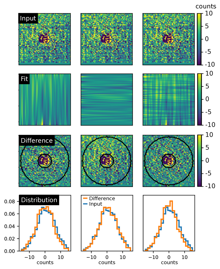
Figure 3: Removal of row and column discontinuities by fitting a third-order polynomial to every row and column.

We introduce a combined method where we model the star and background separately and subtract them from all frames for each wavelength. A flowchart of the method is shown in Fig. 1. We start by subtracting the 99 background frames from the science data to create a stellar PSF model. The additional background noise from the subtraction is much lower than the local stellar photon noise. Therefore, an accurate model of the stellar PSF can be extracted by centering and co-adding the background subtracted frames. The combined images revealed additional structures that are co-moving with the star on the detector. These are an optical ghost arising from the L-band filter and electrical ghosts caused by inter-channel capacitive coupling on the detector (Finger et al., 2008). They are shown in in Fig. 2, in addition to our method to extract these features for the stellar model. We create a mask that surrounds these features for every wavelength bin and only keep the signal that is more than $2\sigma$ compared to the background outside of the mask. Removing the stellar PSF from the science data using this PSF model is now straightforward. We fit a decentered PSF model to background subtracted data frames for each wavelength, retrieving the stellar PSF intensity and the science frames without the stellar PSF.

After masking the planets, we can model the background from the star-subtracted science frames. For every frame we select the frames separated in time by 30 minutes to minimize self-subtraction. We note that the change of the parallactic angle with time during the observations is relatively constant, with 24, 30, and 24 degrees change in three 30 minute windows. From the time separated frames we calculate 10 PCA components. We optimally subtract these components, such that the residuals in the frame are dominated by the photon noise of the star and background. This method of background subtraction results in cubes with a subtracted star and background, where the background is calculated from the science frames themselves. Now, we can check if this method indeed reduces the background noise compared to simply using 10 PCA components of the 99 background frames. By subtracting 10 PCA components from the raw data for both methods, we compare the standard deviation of the residuals after masking the star. Between $2.9$ $\mu$m and $4.2$ $\mu$m, we obtain a reduction of 10% in the standard deviation of the residuals using the background estimate from the on-source frames compared to the background model derived from the off-source frames. Therefore, we use the science data background estimate for all further data reduction.

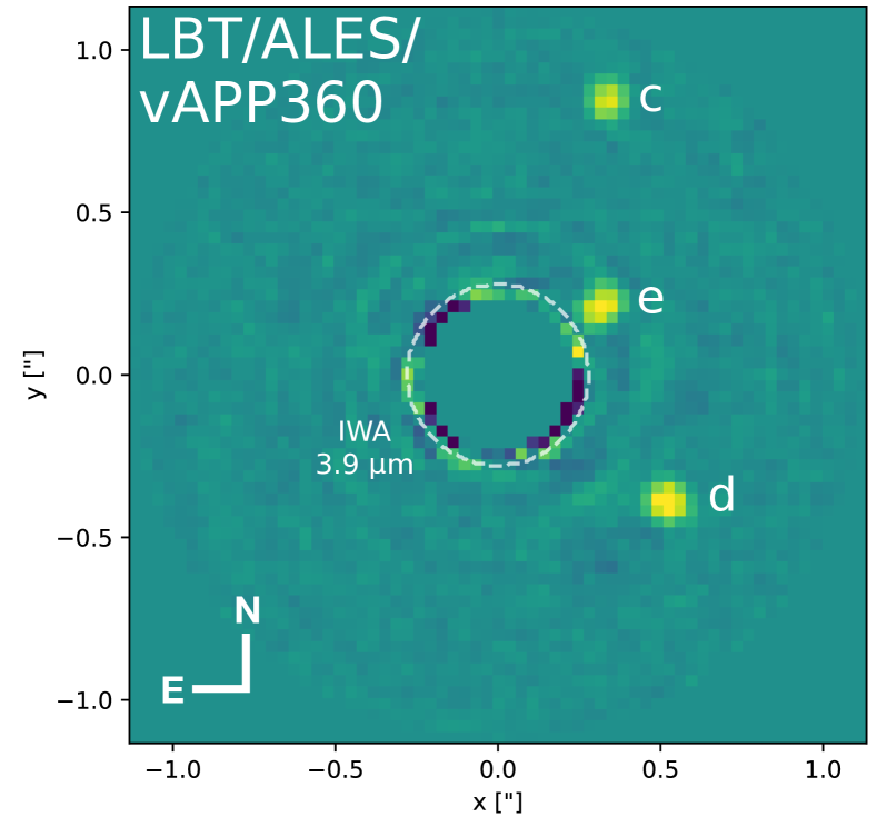
Figure 4: LMIRCam/ALES image of HR 8799 c, d, and e using the dgvAPP360 coronagraph. The final image is the combination of the individual wavelength slices between 3.55-4.15 $\mu$m. North is up, East is left.

We inspect the star- and background-subtracted frames for residual structure by averaging them in time and wavelength. The residuals are not well described by purely Gaussian noise, but contain structures that are column and row specific and vary in time, see Fig. 3. The structures are faint (1-10 counts) and originate from the way in which the ALES microspectra intersect the different channels of the LMIRCam detector. These discontinuities are characterized by fitting polynomials of the third order to each row and column, which are shown in Fig. 3. A third order polynomial is low-order enough over the 65 pixels that it is minimally affected by planet signal, but to be sure we mask the star with an 18 pixel circular mask and the planets with a 5 pixel circular mask and remove those pixels from the fit. Using a Kolmogorov-Smirnov test we verify that both the before and after distributions are non-Gaussian, however we find that the average of the noise distribution is now consistent with zero and the standard deviation of a background region is reduced by 10%. We note that the polynomial background fit has a large number of variables for the full image, but we found it to be the only method that captured the behavior of this phenomenon. Combined with the stellar PSF removal and the background removal, the row and column fits remove most structures present in the data in a way that minimizes self-subtraction of planets.

We center and derotate the background and star subtracted cubes and median stack them along the time axis to create a single master image cube. The final cube is put through a high-pass filter where we remove global structures on the background by subtracting a Gaussian smoothed frame for each wavelength in the final cube. The Gaussian has a standard deviation of 5 pixels (FWHM = 11.8 pixels) and we mask the locations of the HR 8799 planets and the star with NaN values. These NaN values were interpolated over using Astropy.convolve (Astropy Collaboration et al., 2013) to retrieve an estimate of global structures in the background inside the mask.

2.4 Final sensitivity

HR 8799 c, d, and e are detected with high S/N using the combination of ALES with the dgvAPP360. At the location of HR 8799 e there are some residuals from speckles, yet the residuals at the locations of HR 8799 c and d are dominated by the thermal background. HR 8799 b is outside of the field of view of ALES. To estimate our sensitivity we create a crude contrast curve using our data. We focus on the wavelengths where the throughput of the dgvAPP360 is highest, combining images between $3.5$ $\mu$m and $4.15$ $\mu$m. The wavelength-binned image is shown in Fig. 4, where all three planets are clearly visible. At each radius, a ring of subapertures is created, each with diameter of 1.7$\lambda/D$, avoiding the planets when necessary. Flux within each subaperture is summed and the standard deviation of fluxes at each radius is taken as the noise. Contrast is determined by performing similar aperture photometry on the primary star. The resulting contrast curve, not corrected for varying sample size with radius, is shown in Fig. 5, and quickly reaches a noise floor beyond the inner working angle. HR 8799 c, d, and e are detected with S/N ratios of 29, 25 and 19 respectively.

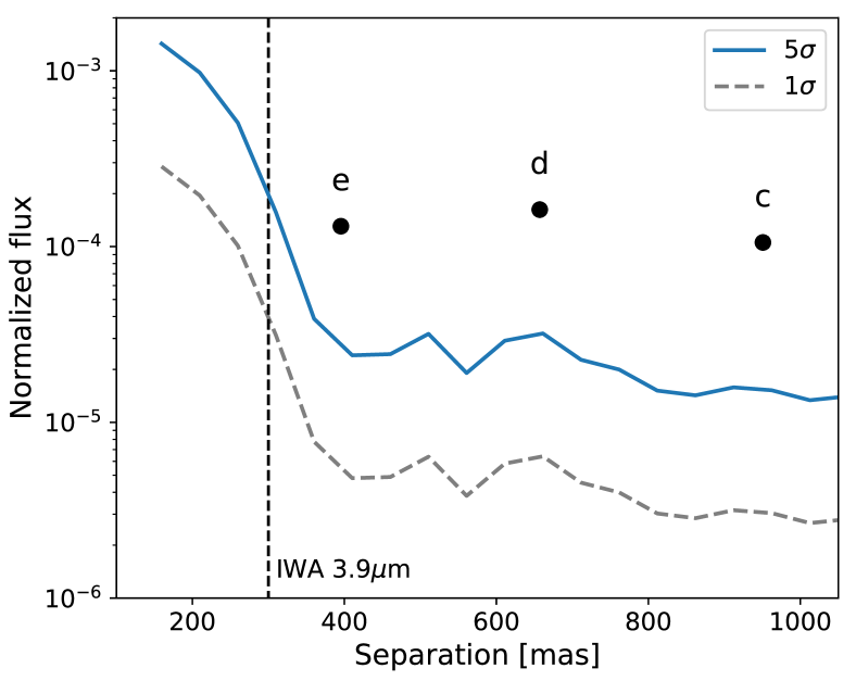
Figure 5: Contrast as a function of separation using LMIRCam/ALES with the dgvAPP360. The background limit is quickly reached outside the inner working angle of the coronagraph.

2.5 Spectral extraction

To extract contrast spectra for each planet from the data, we inject negative planet signals at the locations of the HR 8799 planets in each frame. The injected planets are scaled copies of the stellar PSF at each wavelength. This is a unique strength of the dgvAPP360: we have an unsaturated stellar PSF that acts as a reference PSF for the planets for every science exposure. The planet-subtracted cubes are reduced using the same method described above and in Fig. 1. For each planet and each wavelength bin we optimize the planet location and amplitude by evaluating the Hessian at the planet location in a circular aperture with a diameter of 7 pixels. The Hessian is a measure of the curvature of the image surface, which is minimal when the planet is completely removed (Stolker et al., 2019). Additionally, we find that the distribution of the retrieved locations has a standard deviation of 0.4 pixels for HR 8799 c and d, and 0.6 pixels in HR 8799 e. The resulting flux loss for a PSF that is masked with a circular aperture of 7 pixels with a shift of 0.6 pixels is around 8%. This is smaller than the error bars in the retrieved flux calculated from bootstrapping.

To generate error bars for the retrieved contrast spectra we apply bootstrapping to the data reduction method, selecting 325 frames (with replacement) at random from the data 50 times in total. For the purposes of the bootstrap, the fluxes of the planets for each wavelength are retrieved using aperture photometry, rather than fake planet injection, as the data reduction method is computationally expensive. Assuming that the self-subtraction is similar for all iterations, the distribution of retrieved amplitudes should be a good approximation of the distribution with negative planet injection. The standard deviation of measured fluxes at each wavelength is the $1\sigma$ error due to random noise. Bootstrapping cannot be used to estimate systematic or persistent issues with the data. The scatter seen in the spectrum HR 8799 e, may indicate that the data are influenced by residual speckle noise, especially toward shorter wavelengths.

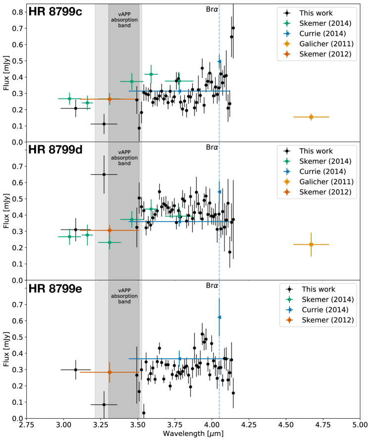
Figure 6: Spectra recovered with negative planet injection for HR 8799 c, d, and e, showing apparent flux. We compare our LMIRCam/ALES spectra to the 3.3 $\mu$m magnitudes from Skemer et al. (2012), the narrow-band magnitudes from Skemer et al. (2014), the broad $L$’-band and [4.05] magnitudes from Currie et al. (2014), and the M-band magnitudes from (Galicher et al., 2011). The light gray and dark gray vertical swaths correspond to the vAPP absorption band, with an absolute transmission of 40% and 25% respectively, as shown in Figure 11.

ALES made no significant detection of any planet between 3.35 $\mu$m and 3.5 $\mu$m due to the absorption of the dgvAPP360 coronagraph (see Appendix A for spectral characterization of the dgvAPP360). We bin the data between 2.99 and 3.17 $\mu$m and 3.17 and 3.35 $\mu$m to retrieve two photometric points for wavelengths short of the dgvAPP360 absorption feature. For this purpose, the negative planet is injected for all wavelength slices separately with a constant spectral slope and the final evaluation of the Hessian is performed on the median combined images. Bootstrapping is applied to find the error on these measurements as well.

We perform flux calibration of the planet contrast spectra by multiplying by a calibrated spectrum of the primary star. We used the SED analyzer VOSA (Bayo et al., 2008) to fit a BT-Settl model to the SED of the host star including data from Tycho2, 2MASS, and WISE (Høg et al., 2000; Cutri et al., 2003; Cutri & et al., 2012). We retrieved a temperature of 7200 K, log(g) = 4 log(cm/s²), a metallicity of 0.5, an $\alpha$ = 0 and a multiplicative dilution factor of 6.416e-19. We smoothed this BT-Settl model to the resolution of ALES and sampled it at the same wavelengths as our final cube. We then multiply this calibrated smoothed and sampled spectrum of the star by the contrast spectra of the planets to yield flux calibrated spectra of HR 8799 c, d, and e. The retrieved spectra can be found in Appendix B.

2.6 Comparison to other measurements in the band

Figure 6 compares our ALES measurements with previous thermal-IR measurements in the literature for HR 8799 c, d, and e. To quantitatively compare our ALES measurements to literature measurements with wider bandwidths than our spectral channels, we calculate synthetic photometry using our ALES spectra and cryogenic filter traces provided by the Spanish Virtual Observatory (Rodrigo et al., 2012; Rodrigo & Solano, 2020). Since the NIRC2 $L^{\prime}$ band extends into the vAPP absorption band where we do not have ALES measurements, we interpolate through the vAPP absorption band to the $3.1~{}\mu\mathrm{m}$ synthetic photometry point. This is a reasonable interpolation because Skemer et al. (2014) observed no significant absorption through these wavelengths. We cannot synthesize a photometric measurement for the Br-$\alpha$ narrowband filter photometry presented by Currie et al. (2014), or for the LNB1 and LNB2 filters presented by Skemer et al. (2014) as these filters all have narrower bandwidths than the ALES spectral channels.

We use a Monte Carlo approach to propagate correlated uncertainty in the ALES measurements to the synthetic photometry. First, the spectrum of each planet is modeled as a multi-dimensional Gaussian distribution with means determined by our spectra and covariance estimated using the method of Greco & Brandt (2016). Next, photometry is measured for each of 100 draws from these distributions and the uncertainty taken as the standard deviation of the measurements. Table 1 lists the results.

Our flux scaling and photometry for the system is consistent with photometry presented by Currie et al. (2014), the ALES $L^{\prime}$ measurements appearing a bit low for planet c, a bit high for planet d, and nearly the same for planet e. For planets c and d, we can also compare to the LMIRCam-LNB5 and LNB6 measurements from Skemer et al. (2014). For planet c there exists some tension, with the ALES measurements fainter by 2.35$\sigma$ and 1.95$\sigma$ for LNB5 and LNB6, respectively. For planet d, the ALES measurements seem consistent with the previous results.

Table 1: Comparing to Photometry

Filter	ALES synth. phot.	Lit. phot.	Difference
	(mJy)	(mJy)	($\sigma$)
planet c
NIRC2-$L^{\prime}$	$0.286\pm 0.01$	$0.337\pm 0.02$	-1.8
LMIRCam-LNB5	$0.273\pm 0.02$	$0.435\pm 0.06$	-2.35
LMIRCam-LNB6	$0.271\pm 0.01$	$0.392\pm 0.05$	-1.95
planet d
NIRC2-$L^{\prime}$	$0.437\pm 0.02$	$0.387\pm 0.03$	1.6
LMIRCam-LNB5	$0.366\pm 0.02$	$0.436\pm 0.06$	-1.12
LMIRCam-LNB6	$0.421\pm 0.01$	$0.393\pm 0.05$	0.53
planet e
NIRC2-$L^{\prime}$	$0.350\pm 0.07$	$0.395\pm 0.055$	-0.48

3 Atmospheric model fitting

3.1 Compiling low-resolution data

In combination with these ALES spectra, low resolution integral field spectroscopy has measured the z, J, H, K, and L band emission from HR 8799 c, d, and e. We fit model atmosphere spectra to these data, and, when available, we include photometric measurements between and beyond the bands covered by spectroscopy. For all the planets, measurements with a signal to noise less than unity were clipped, and covariance matrices for IFS data were generated following the approach outlined by Greco & Brandt (2016). We assumed that the significant binning required to produce the ALES synthetic photometry point decoupled that point from the rest of the ALES spectra.

Below we briefly summarize the data compilations for each planet.

3.1.1 Planet c data

We combined our ALES measurements with the Project-1640 zJ band measurements (we used the version extracted with a PCA-based image post processing algorithm Oppenheimer et al., 2013) and included the GPI H and K band measurements (Greenbaum et al., 2018). For the GPI measurements, we clipped data in the overlapping region of the K1 and K2 filters (removing the last three points in the K1 spectrum and the first eight points of K2). The LBTI/LMIRCam LNB1, LNB2, and LNB3 measurements from Skemer et al. (2014) were used in place of the binned ALES measurements between 2.99 $\mu\mathrm{m}$ and 3.36 $\mu\mathrm{m}$ because they provide finer wavelength sampling and higher precision. The Keck/NIRC2 $M$-band measurement from Galicher et al. (2011) was also included.

3.1.2 Planet d data

For planet d, we combined our ALES measurements with the SPHERE IFS YH band measurements (Zurlo et al., 2016) and the GPI H and K-band measurements (Greenbaum et al., 2018). We clipped the SPHERE data at the red end in order to not overlap with the GPI H band measurements and clipped the GPI K1 and K2 spectra in the overlapping region, removing the last three points of K1 and the first eight points of K2. The LBTI/LMIRCam LNB1, LNB2, and LNB3 measurements from Skemer et al. (2014) were used in place of the binned ALES measurements between 2.99 $\mu\mathrm{m}$ and 3.36 $\mu\mathrm{m}$ because they provide finer wavelength sampling and higher precision.The Keck/NIRC2 $M$-band measurement from Galicher et al. (2011) were included.

3.1.3 Planet e data

For planet e, we combined our ALES measurements with the SPHERE IFS YH band measurements (Zurlo et al., 2016) and the GPI H and K-band measurements (Greenbaum et al., 2018). We clipped the SPHERE data at the red end in order to not overlap with the GPI H band measurements, and clipped the GPI K1 and K2 spectra in the overlapping region, removing the last three points in of K1 and the first eight points of K2. The 2.99 $\mu\mathrm{m}$ to 3.17 $\mu\mathrm{m}$ ALES synthetic photometry point is included, as this bin appears consistent with previous observations for planets c and d. The 3.17 $\mu\mathrm{m}$ to 3.36 $\mu\mathrm{m}$ ALES synthetic photometry point is not used because this measurement appears to be affected by poor transmission through the dgvAPP360.

3.2 Fitting Approach

We fit synthetic spectra from three distinct families of models to the measurements of each planet. The models were: 1) blackbodies; 2) DRIFT-Phoenix models (Witte et al., 2011), which use a microphysics-based cloud prescription and provide subsolar, solar, and supersolar metallicities; and 3) solar metallicity Phoenix-based models with a parameterized cloud (Barman et al., 2015; Brock et al., 2021). The $P_{\mathrm{c.t.}}$ parameter of the Barman/Brock models is the pressure below which cloud particle density declines exponentially. The median grain size and the eddy diffusion coefficient used for the Barman/Brock models are $1~{}\mu\mathrm{m}$ and $10^{8}~{}\mathrm{cm}^{2}\mathrm{s}^{-1}$, respectively. The parameter ranges and step sizes for each grid are summarized in Table 2.

The models were interpolated to provide finer sampling of their parameters using multi-dimensional linear interpolation after rescaling input parameters to the unit cube. For the synthetic atmosphere models we created 10 K steps in effective temperature and steps of 0.1 dex in surface gravity. For the DRIFT models, we created 0.1 dex steps in metallicity. For the Barman/Brock models, we created 0.3 dex steps in the pressure below which cloud particle density decays exponentially. Blackbody models were precomputed with 2 K steps.

Table 2: Description of Model Libraries Used

Parameter	Barman/Brock	DRIFT	Blackbody	Comments
$T_{\mathrm{eff}}$ range	800–1500 K	1000–1500 K	800–1500 K	100 K gridpoints interpolated to 10 K steps
$\log(\frac{g}{\mathrm{cms}^{-2}})$ range	3.5–5.0	3.5–5.0	$\cdots$	0.5 dex gridpoints interpolated to steps of 0.1
$\log(\frac{z}{z_{\odot}})$ range	$\cdots$	-0.3–0.3	$\cdots$	0.5 dex gridpoints interpolated to steps of 0.1
$P_{\mathrm{c.t.}}$	0.5, 1, 2, 4	$\cdots$	$\cdots$	bars, the 2 bar model is interpolated

Table 3: Model Fits to HR 8799 c, d, e

Parameter	planet c	planet d	planet e
Barman/Brock Phoenix Models
$T_{\mathrm{eff}}$ [K]	1240	1140	1140
$\log(\frac{g}{\mathrm{cm}\cdot\mathrm{s}^{2}})$	3.6	3.6	3.8
$P_{\mathrm{ct}}$ [bar]	2	1	0.5
$R$ [$R_{\mathrm{Jup}}$]	0.91	1.27	1.19
$\log(\frac{L_{\mathrm{bol}}}{L_{\odot}})$	-4.71	-4.62	-4.61
$\chi^{2}$	234	1357	1379
degrees of freedom	163	169	149
DRIFT Phoenix Models
$T_{\mathrm{eff}}$ [K]	1500	1430	1480
$\log(\frac{g}{\mathrm{cm}\cdot\mathrm{s}^{2}})$	3.5	3.5	3.9
$\log(\frac{z}{z_{\odot}})$	0.3	-0.3	-0.3
$R$ [$R_{\mathrm{Jup}}$]	0.65	0.75	0.66
$\log(\frac{L_{\mathrm{bol}}}{L_{\odot}})$	-4.67	-4.64	-4.67
$\chi^{2}$	485	1933	1841
degrees of freedom	163	169	149
Blackbody Models
$T_{\mathrm{eff}}$ [K]	1424	1516	1620
$R$ [$R_{\mathrm{Jup}}$]	0.75	0.62	0.5
$\log(\frac{L_{\mathrm{bol}}}{L_{\odot}})$	-4.65	-4.69	-4.70
$\chi^{2}$	664	4323	3745
degrees of freedom	165	171	151

Prior to fitting, model spectra were preprocessed to match the characteristics of each instrument. This included smoothing to R=33 for fits to P1640 and SPHERE spectra. For the GPI spectra we used the method presented in Stone et al. (2016) to smooth the models with a linearly increasing spectral resolution going from R=45 to R=80 from the beginning of H-band to the end of K2. ALES data were fit with models smoothed to R=20. After smoothing, all model spectra were sampled at the wavelengths provided by each instrument. We also preprocessed photometry for the LMIRCam/LNB1, LNB2, LNB3, and the NIRC2 $M$-band points used.

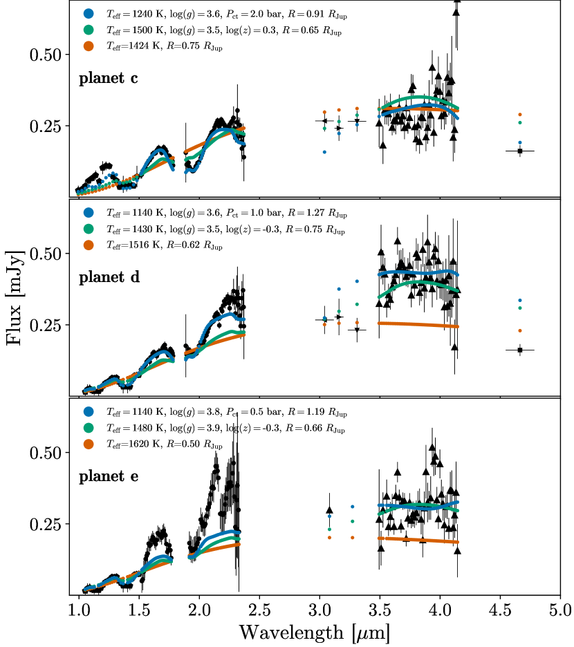
Figure 7: The measured portions of the spectral energy distributions for planets HR 8799 c, d, and e (black markers, data source-eps-converted-to.pdfs described in the text). Colored markers indicate best fit model spectra from three model families. Blue points are from the Barman/Brock Phoenix models. Teal points show DRIFT-Phoenix models, and orange points are blackbodies.

Data were fit using a Gaussian likelihood function, treating each band, $i$, individually

$$\mathcal{L}_{i}(\theta,R,\varpi))\propto\\ \mathrm{exp}\left(-\frac{1}{2}((R\varpi)^{2}x(\theta)-\mu_{i})^{T}\Sigma_{i}^{-1}((R\varpi)^{2}x(\theta)-\mu_{i})\right),$$ (1)

where $\theta$ represents a vector of model parameters for the given model family, $R$ is the object radius, $\varpi$ is the system parallax, and $\mu_{i}$ and $\Sigma_{i}$ are the measured data and covariance matrix for the given spectrum or photometric measurement. We performed our fit using a grid-based approach that facilitated the construction of a global likelihood function through multiplication grid-cell by grid-cell

$$\mathcal{L}(\theta,R,\varpi)=\prod_{i}\mathcal{L}_{i}(\theta,R,\varpi)).$$ (2)

We multiplied our likelihood grids by priors for each fitted parameter. For each model family we used a log-uniform prior on $R$, extending from 0.5 to 2 $R_{\mathrm{Jup}}$, and a Gaussian prior on $\varpi$ using the $Gaia$ measurement and uncertainty ($24.46\pm 0.045$ mas) as the mean and standard deviation, respectively Gaia Collaboration et al. (2018). For $T_{\mathrm{eff}}$, $\log(g)$, and $\log(z)$ a uniform prior was used. The prior for $P_{\mathrm{c.t.}}$ was log-uniform.

3.3 Model Fitting Results

Table 3 lists and Figure 7 displays our fitting results. The Barman/Brock set of models, with greater cloud flexibility, can provide reasonably close fits to the observations of planets c and d. Neither the DRIFT models nor the Barman/Brock models fit planet e particularly well, the H and K-bands being especially hard. As expected, the black-body models provide a poor fit to the spectrum of each planet. For each planet, best fit models align most closely with the data having smallest uncertainty, consistent with expectations. For HR 8799 c, since the GPI data has the smallest uncertainty (and densest sampling), the optimal models prefer to fit the H and K bands even if it costs a poorer fit through the z, J, and L bands. For HR 8799 d, and e the SPHERE data has the smallest uncertainty, so optimal models prefer to fit the z and J bands even if it costs a poorer fit through the H, K, and L-bands.

Systematic differences between the models dominate our parameter uncertainty. While within a model family, allowed parameter ranges (that is, the $\Delta\chi^{2}$=1 surface) typically span only one grid-cell, between the different models temperatures for planet c span $\sim 1200$ to $1500~{}\mathrm{K}$, temperatures for planet d span $\sim 1100$ to $1400~{}K$, and temperatures for planet e span $\sim 1100$ to $1600~{}\mathrm{K}$. Surface gravity has less variance between the models, constrained at the 0.1 dex level. Best fit planet radii span 0.65 to 0.91 $R_{\mathrm{Jup}}$ for planet c, 0.62 to 1.27 $R_{\mathrm{Jup}}$ for planet d, and 0.5 to 1.19 $R_{\mathrm{Jup}}$ for planet e.

Table 3 reports the inferred bolometric luminosity of each planet. To derive the planet luminosity, a hybrid approach was employed utilizing observed flux measurements wherever possible and integrating under the best-fit model atmosphere at wavelengths between and beyond the measured bands. The uncertainty in the luminosity estimate is dominated by the choice of atmospheric model family, yet the resulting values span only 0.09 dex, a very small uncertainty compared to the predictions of evolutionary models —resulting in a mass error of $\lesssim 1~{}M_{\mathrm{Jup}}$ for a given age, or an age error of less than 10 Myr for a given mass for the (Baraffe et al., 2003, See Figure 8). The result suggests that luminosity is not particularly sensitive to the choice of well scaled model, especially in this case where we have broad wavelength coverage near the peak of each planet’s spectral energy distribution.

4 Discussion

Hot-start evolutionary models predict a very narrow range of effective temperatures, surface gravity, and planetary radius constrained by the fundamental parameters of the HR 8799 planets. Constrained parameters include system age ($33^{+7}_{-13}$ Myr or $90^{381}_{-50}$ Myr, Baines et al., 2012), planet mass (planets c and d $\lesssim 10~{}M_{\mathrm{Jup}}$, planet e $9.6^{+1.9}_{-1.8}~{}M_{\mathrm{Jup}}$, Fabrycky & Murray-Clay, 2010; Brandt et al., 2021), and bolometric luminosity (Table 3).

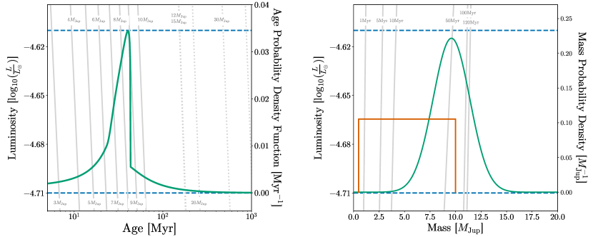
Figure 8: Left: Luminosity versus age. The gray curves represent the predictions of the Baraffe et al. (2003) evolutionary models. Blue horizontal lines indicate the luminosity constraints for the HR 8799 planets. The green curve corresponds to the right axis and shows the system age probability distribution function giving equal weight to the contracting and expanding scenarios from Baines et al. (2012). Right: Luminosity versus mass. Gray curves are from the evolution model. Blue horizontal lines indicate the luminosity constraints. The orange and green curves correspond to the right axis and indicate probability distribution functions derived from stability arguments (orange) and from the astrometric influence of planet e (green).

To illustrate this we used the ‘evolve’ module of the SpeX Prism Library Analysis Toolkit (SPLAT, Burgasser & Splat Development Team, 2017) to construct a distribution of evolution model predictions for effective temperature, surface gravity, and radius. We used a Monte Carlo approach to build distributions for four different models (Burrows et al., 2001; Saumon & Marley, 2008; Baraffe et al., 2003). 1.2 million age-mass points were input into the evolutionary models and the output discarded if the returned luminosity was outside the measured range. For the system age, we modeled each of the ranges indicated by Baines et al. (2012) using a generalized extreme value distribution (Possolo et al., 2019), giving equal weight to the younger and the older ranges. Planet masses were sampled from a uniform distribution spanning 0.5 to 10 $M_{\mathrm{Jup}}$, consistent with dynamical constraints (e.g., Fabrycky & Murray-Clay, 2010). Since the allowed luminosity ranges for each planet are similar, we used a single range for all planets, spanning $\log_{10}(\frac{L_{\mathrm{bol}}}{L_{\odot}})$=-4.71 to -4.61. The intersection of these constraints on the Baraffe et al. (2003) evolutionary models are plotted in Figure 8 as an example.

The results of our Monte Carlo sampling are displayed in Figure 9. We repeated the sampling exercise using a Gaussian distributed mass constraint approximating the results of Brandt et al. (2021, $M=9.6\pm 1.8~{}M_{\mathrm{Jup}}$) and no significant change to the resulting distributions resulted.

The predictions of gas-giant evolution models are sensitive to the initial entropy assumed during early times. For 10 $M_{\mathrm{Jup}}$ objects hot-start and cold-start evolutionary models do not converge for $\sim 1$ Gyr (less massive objects converge faster Marley et al., 2007). Each of the four models we use assume hot-start evolution. Hot start models are consistent with initial entropy constraints for the planets Marleau & Cumming (2014), however ”warm”-start models are also allowed.

Assuming hot-start evolution, Figure 9 suggests $T_{\mathrm{eff}}\approx 1075$ K, $\log(g)\approx 4.1$, and $R\approx 1.29~{}R_{\mathrm{Jup}}$. Comparing to Table 3 we see that the best-fit Barman/Brock Phoenix models provide reasonable parameters for HR 8799 d and HR 8799 e, with $T_{\mathrm{eff}}$ within 100 K, $\log(g)$ within 0.5 dex, and plausible planet radii. The best-fit for HR 8799 c has more tension with the evolutionary models, suggesting a radius of 0.91 $R_{\mathrm{Jup}}$. The best-fit DRIFT models have temperatures much higher (and radii much smaller) than predicted by evolution models.

Given the narrowly peaked distributions in Figure 9, we re-ran our fitter, fixing $T_{\mathrm{eff}}=1075$ K and $\log(g)$=4.1. We fit twice, using different constraints on planet radius each time. First, we restricted $R$ to be within 1.25 and 1.45 $R_{\mathrm{Jup}}$. Second we fixed $R$ at 1.29 $R_{\mathrm{Jup}}$. We also used more flexible models, now exposing both cloud top pressure and median grain size as tunable parameters. Our question was: Assuming evolutionary models are correct, what does that imply about the physical state of the atmosphere? The results are shown in Figure 10.

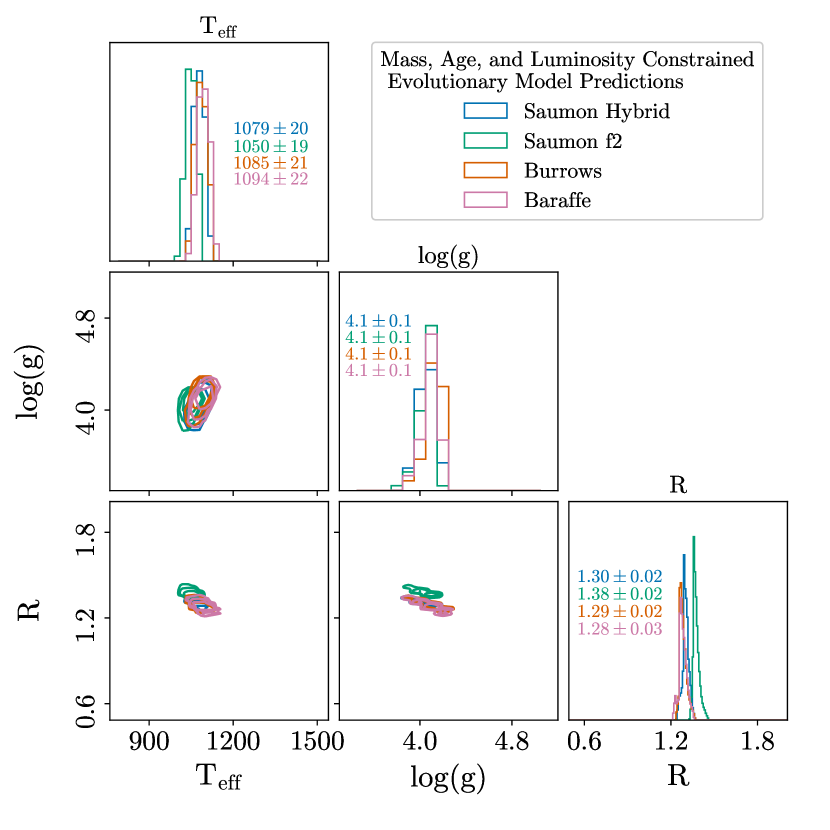
Figure 9: Temperature, surface gravity, and radius predictions from four hot-start evolutionary models, given the age, mass, and luminosity constraints for HR 8799 c, d, and e. Predictions are narrowly peaked and are relatively model independent.

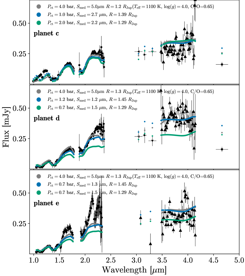
Figure 10: The measured portions of the spectral energy distributions for planets HR 8799 c, d, and e (black markers, data sources described in the text). Barman/Brock Phoenix models with temperature and surface gravity fixed at the values predicted by hot-start evolutionary models ($T_{\mathrm{eff}}=1075$ K, $\log(g)=4.1$) are fit to the data by varying two cloud parameters. Blue points are for a fit letting the radius float between 1.25 and 1.45 $R_{\mathrm{Jup}}$. Teal points show a fit where radius is fixed to $1.29~{}R_{\mathrm{Jup}}$. Thick clouds with small grains are preferred for each planet, suggesting such conditions are necessary to bring atmospheric models and evolutionary models into agreement. We also show the $T_{\mathrm{eff}}=1100$ K, $\log(g)=4$, Phoenix model presented by Konopacky et al. (2013) and Greenbaum et al. (2018) (gray markers). This model is also consistent with the evolutionary model predictions. It was drawn from the same Barman/Brock family of models presented here but includes a supersolar C/O ratio.

By adjusting both the cloud top pressure and the median grain size, we are able to find reasonably good fits to the data at the expected temperature and surface gravity. In all cases, small median grain-size, $<3~{}\mu\mathrm{m}$, are preferred. HR 8799 e is fit with the most extended cloud, but this planet is also the least well matched by the models, the H and K-band spectra are systematically under predicted. Given that HR 8799 e is the closest-in and hardest to observe planet, it is hard to distinguish persistent systematic issues with the spectroscopy from deficiencies of the model atmospheres and probably both are at play. For HR 8799 d, as seen in the middle panel of Figure 10, the fixed $R=1.29~{}R_{\mathrm{Jup}}$ fit is a poor match to the data, especially compared to the more flexible constrained fit and the unconstrained fit.

Additional atmospheric model parameters are necessary to provide improved fits. In Konopacky et al. (2013) a Phoenix model from the same family as the Barman/Brock models used here is fit to higher resolution K-band spectroscopy of HR 8799 c. The atmospheric model, with $T_{\mathrm{eff}}=1100$ K and $\log(g)=4.0$, is consistent with the predictions of hot-start evolution models, and matches low-resolution spectroscopy and the broadband SED reasonably well (Greenbaum et al., 2018). In addition to cloud top pressure and median grain size, the Konopacky et al. (2013) model also adjusts the C/O ratio in the planetary atmosphere. Figure 10 compares our results with the Phoenix model of Konopacky et al. (2013).

Our analysis does not utilize models with a cloud coverage/patchiness parameter, yet some previous studies suggest that this may be important for the HR 8799 planets (e.g., Currie et al., 2014; Skemer et al., 2014). For HR 8799 c, our fits in Figures 7 and 10 show that matching the zJ band emission while simultaneously fitting longer wavelengths is challenging. One way to enhance emission from the z through J bands is with cloud patches (Marley et al., 2010).

5 Conclusion

New coronagraphic L-band integral field spectroscopy of the HR 8799 system are presented using the LMIRCam/ALES instrument and a double-grating vector apodizing phase plate. These are the first L-band spectroscopic measurements of HR 8799 d and e, and the first broadband spectroscopy of HR 8799 c at these wavelengths. Our measurements are generally consistent with earlier photometric probes covering portions of this band, although there is some tension with Skemer et al. (2014) for HR 8799 c.

Atmospheric model fits incorporating a parameterized treatment of clouds can provide a reasonable fit to the 1-4.6 $\mu\mathrm{m}$ spectral energy distribution of the planets when the median grain size is small. HR 8799 d is particularly well fit with atmospheric models that agree with the predictions of hot-start evolutionary models.

An approach of sampling evolution models is developed to create distributions of predicted temperature, gravity, and radius given constraints on several fundamental parameters of the HR 8799 system. Re-running of fits fixing these parameters enables the use of a more flexible synthetic atmosphere model.

While evolution models depend on initial conditions for ages $\lesssim 1$ Gy, our approach can be applied to older systems where ambiguity about the formation path is less of an issue. Powerful thermal-IR instruments, such as LMIRCam/ALES, are capable of direct imaging observations of older planets, which maintain their thermal-IR flux even as the near-IR fades dramatically. Future facilities like JWST and the next generation of 30-m class telescopes with mid-IR instruments such as METIS (Brandl et al., 2021) and PSI-red (Skemer et al., 2018b) will extend this capability to fainter/older targets. When paired with the power of Gaia to find and constrain the masses of wide orbit planets, in future studies we will be well equipped to make use of evolutionary models to provide quantitative priors for their atmospheric model fitting.

Appendix A Characterization of the dgvAPP360.

The double grating vector apodizing phase plate 360 (dgvAPP360) was installed in LMIRCam early September 2018. The design and first-light results are presented in Doelman et al. (2020). Observations of the PDS 201 system using this dgvAPP360 show that the vAPP has an improved sensitivity of a factor two compared to non-coronagraphic imaging in the regions closest to the star (450-800 mas) (Wagner et al., 2020). Here we provide further characterization of the dgvAPP360 performance, focusing on the throughput as a function of wavelength.

The double-grating vAPP has two separate liquid-crystal layers, an additional glue layer and an extra substrate compared to a standard gvAPP (Doelman et al., 2017, 2020). These additional layers lead to extra absorption, specifically in the $3.24$-$3.5$ $\mu$m range, where both the liquid-crystal molecules and the glue molecules have an infra-red absorption feature due to carbon-carbon bonds (Otten et al., 2017). Because these features are in the spectral range of ALES, we conduct an experiment to measure their impact. We disperse the coronagraphic (vAPP) PSF and non-coronagraphic (clear pupil) PSF using a grism in tandem with the $L$-Spec filter, using only the left aperture (SX) of the internal pupil mask. The dispersed PSFs are shown in Fig. 11.

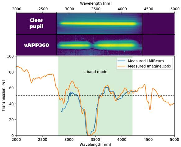
Figure 11: Transmission measurements of the vAPP in the 2.8-4.2 $\mu$m range using a grism to disperse the vAPP and non-coronagraphic PSF.

In addition, we obtain narrow band images at $2.9$ $\mu$m, $3.3$ $\mu$m, $3.5$ $\mu$m, and $3.9$ $\mu$m that are used for wavelength calibration. Because the pupil selection mask is in the same filter wheel as the narrow band filters, the narrow band images are the coherent sum of both pupils, creating Fizeau fringes. We remove this effect for our wavelength calibration by summing the flux in 100 pixels in the fringe direction. We fit a Gaussian to the one-dimensional sum of each wavelength to retrieve accurate centroids. We then use the centroids to calculate the wavelength solution of the dispersion.

Calculating the transmission of the vAPP is complicated by the difference in intrinsic Strehl between the two PSFs. The vAPP has an intrinsic Strehl of 46% and the PSF core is slightly broadened due to the apodization by the vAPP in the pupil plane. We retrieve the throughput by forward modelling both PSFs for the full bandwidth. For continuous wavelength coverage, we generate a wavelength-scaled PSF every 2 pixels in the image, corresponding to an average spectral resolution of 10 nm. The model PSF is the incoherent sum of all individual PSFs with an individual scale factor. We minimize the difference between the simulated and measured PSF by changing these scale factors, thereby retrieving the true input spectrum. The final transmission is the optimized vAPP spectrum divided by the non-coronagraphic spectrum, and is shown in Fig. 11. We compare the results with the transmission that is measured by the manufacturer. The curves are in good agreement except for the transmission between 2.9 and 3.2 micron. It is unclear what causes the difference of more than 10% in this spectral bin, compared to the LMIRCam average transmission of 47%. A significant fraction of the spectral band is unavailable when using the vAPP because of the absorption feature. Specifically, the absorption is centered on a spectral feature of CH₄. While this inhibits the detection of methane in the atmospheres of L-type gas giants, cooler gas giants with more CH₄ will have a measurable spectral slope between 3.5-4.1 $\mu$m, where the average transmission of the vAPP is 51%.

Appendix B Tabulated Planet Spectra

Table 4: ALES spectra of HR 8799 c, d, and e

Wavelength	Planet c flux	Planet c flux uncertainty	Planet d flux	Planet d flux uncertainty	Planet e flux	Planet e flux uncertainty
(micons)	(mJy)	(mJy)	(mJy)	(mJy)	(mJy)	(mJy)
3.081	0.2078	0.0536	0.3101	0.0713	0.2984	0.0597
3.272	0.1115	0.0614	0.6491	0.1169	0.0842	0.0831
3.493	0.2594	0.0848	0.3242	0.1215	0.2654	0.1754
3.509	0.0861	0.0892	0.5048	0.0953	0.1647	0.0605
3.525	0.1822	0.0659	0.4510	0.0598	0.2986	0.0615
3.540	0.3052	0.0503	0.4271	0.0571	0.0333	0.0557
3.556	0.2967	0.0420	0.3218	0.0464	0.3469	0.0581
3.571	0.2916	0.0422	0.3553	0.0383	0.2400	0.0325
3.586	0.3143	0.0479	0.3385	0.0353	0.2753	0.0513
3.601	0.2443	0.0279	0.3830	0.0415	0.3096	0.0450
3.616	0.2690	0.0425	0.4038	0.0364	0.2403	0.0284
3.631	0.2668	0.0467	0.4258	0.0389	0.3487	0.0381
3.646	0.2842	0.0338	0.5437	0.0484	0.4311	0.0355
3.660	0.3135	0.0456	0.4506	0.0598	0.3433	0.0265
3.675	0.2659	0.0346	0.4689	0.0432	0.2420	0.0241
3.689	0.2846	0.0290	0.4590	0.0586	0.3296	0.0301
3.704	0.2434	0.0406	0.4452	0.0412	0.3295	0.0282
3.718	0.3126	0.0391	0.4194	0.0345	0.1988	0.0276
3.732	0.2514	0.0290	0.4327	0.0508	0.2697	0.0317
3.746	0.2788	0.0402	0.4573	0.0465	0.3248	0.0325
3.760	0.3766	0.0545	0.3540	0.0426	0.2621	0.0272
3.774	0.3901	0.0382	0.4274	0.0459	0.2842	0.0439
3.788	0.2463	0.0402	0.3886	0.0379	0.2732	0.0369
3.802	0.2038	0.0426	0.4995	0.0533	0.2888	0.0431
3.815	0.2525	0.0369	0.4869	0.0466	0.3122	0.0526
3.829	0.1946	0.0421	0.3630	0.0450	0.3213	0.0520
3.842	0.2813	0.0454	0.3975	0.0645	0.2657	0.0525
3.856	0.2780	0.0356	0.5138	0.0601	0.1936	0.0608
3.869	0.3239	0.0379	0.3785	0.0845	0.3054	0.0575
3.882	0.2110	0.0498	0.4156	0.0730	0.4325	0.0938
3.895	0.2439	0.0571	0.5400	0.0953	0.3248	0.0689
3.908	0.3220	0.0876	0.4696	0.0619	0.3148	0.0500
3.921	0.2872	0.0450	0.4135	0.0429	0.3405	0.0760
3.934	0.4545	0.0598	0.3760	0.0647	0.5182	0.0680
3.947	0.2267	0.0495	0.4902	0.0434	0.4687	0.0509
3.960	0.3507	0.0442	0.5168	0.0584	0.4867	0.0654
3.973	0.3741	0.0485	0.4035	0.0659	0.3334	0.0456
3.985	0.4246	0.0678	0.4740	0.0892	0.2675	0.0354
3.998	0.3697	0.0523	0.3944	0.0522	0.4600	0.0503
4.010	0.2847	0.0473	0.3899	0.0497	0.3536	0.0508
4.023	0.3388	0.0606	0.4036	0.0679	0.3208	0.0597
4.035	0.2933	0.0566	0.3124	0.0819	0.2460	0.0642
4.048	0.3333	0.0785	0.4057	0.0755	0.3103	0.0398
4.060	0.4194	0.0842	0.3149	0.0543	0.3127	0.0459
4.072	0.3649	0.0785	0.4215	0.1421	0.2336	0.0372
4.084	0.4044	0.0662	0.3252	0.1486	0.3682	0.0635
4.096	0.4092	0.1552	0.3696	0.0943	0.3655	0.0716
4.108	0.2094	0.0841	0.4724	0.1497	0.2363	0.0649
4.120	0.2367	0.0817	0.1724	0.0959	0.2806	0.0799
4.132	0.6473	0.1246	0.3555	0.1159	0.3597	0.1081
4.144	0.7018	0.1879	0.3727	0.2420	0.1557	0.0930

Table 5: Spectral correlation parameters for ALES spectra of HR 8799 planets

Planet	$A_{\rho}$	$\sigma_{\rho}$	$A_{\lambda}$	$\sigma_{\lambda}$	$A_{\delta}$
c	1.24E-2	1.61E02	3.95E-1	2.42E-3	5.94E-1
d	1.17E-2	1.02E03	4.09E-1	2.47E-3	5.81E-1
e	2.92E-2	1.36E04	1.24E-1	2.57E-2	8.47E-1

Note. — Parameters as defined by Greco & Brandt (2016)

References

- Astropy Collaboration et al. (2013) Astropy Collaboration, Robitaille, T. P., Tollerud, E. J., et al. 2013, A&A, 558, A33
- Baines et al. (2012) Baines, E. K., White, R. J., Huber, D., et al. 2012, ApJ, 761, 57
- Baraffe et al. (2003) Baraffe, I., Chabrier, G., Barman, T. S., Allard, F., & Hauschildt, P. H. 2003, A&A, 402, 701
- Barman et al. (2015) Barman, T. S., Konopacky, Q. M., Macintosh, B., & Marois, C. 2015, ApJ, 804, 61
- Barman et al. (2011) Barman, T. S., Macintosh, B., Konopacky, Q. M., & Marois, C. 2011, ApJ, 733, 65
- Bayo et al. (2008) Bayo, A., Rodrigo, C., Barrado Y Navascués, D., et al. 2008, A&A, 492, 277
- Bonnefoy et al. (2016) Bonnefoy, M., Zurlo, A., Baudino, J. L., et al. 2016, A&A, 587, A58
- Brandl et al. (2021) Brandl, B., Bettonvil, F., van Boekel, R., et al. 2021, The Messenger, 182, 22
- Brandt et al. (2021) Brandt, G. M., Brandt, T. D., Dupuy, T. J., Michalik, D., & Marleau, G.-D. 2021, ApJ, 915, L16
- Briesemeister et al. (2018) Briesemeister, Z., Skemer, A. J., Stone, J. M., et al. 2018, in Society of Photo-Optical Instrumentation Engineers (SPIE) Conference Series, Vol. 10702, Ground-based and Airborne Instrumentation for Astronomy VII, ed. C. J. Evans, L. Simard, & H. Takami, 107022Q
- Brock et al. (2021) Brock, L., Barman, T., Konopacky, Q. M., & Stone, J. M. 2021, ApJ, 914, 124
- Burgasser & Splat Development Team (2017) Burgasser, A. J., & Splat Development Team. 2017, in Astronomical Society of India Conference Series, Vol. 14, Astronomical Society of India Conference Series, 7–12
- Burrows et al. (2001) Burrows, A., Hubbard, W. B., Lunine, J. I., & Liebert, J. 2001, Reviews of Modern Physics, 73, 719
- Currie et al. (2011) Currie, T., Burrows, A., Itoh, Y., et al. 2011, ApJ, 729, 128
- Currie et al. (2014) Currie, T., Burrows, A., Girard, J. H., et al. 2014, ApJ, 795, 133
- Cutri & et al. (2012) Cutri, R. M., & et al. 2012, VizieR Online Data Catalog, II/311
- Cutri et al. (2003) Cutri, R. M., Skrutskie, M. F., van Dyk, S., et al. 2003, VizieR Online Data Catalog, II/246
- Doelman et al. (2020) Doelman, D. S., Por, E. H., Ruane, G., Escuti, M. J., & Snik, F. 2020, PASP, 132, 045002
- Doelman et al. (2017) Doelman, D. S., Snik, F., Warriner, N. Z., & Escuti, M. J. 2017, in Society of Photo-Optical Instrumentation Engineers (SPIE) Conference Series, Vol. 10400, Society of Photo-Optical Instrumentation Engineers (SPIE) Conference Series, 104000U
- Doelman et al. (2021) Doelman, D. S., Snik, F., Por, E. H., et al. 2021, Appl. Opt., 60, D52
- Fabrycky & Murray-Clay (2010) Fabrycky, D. C., & Murray-Clay, R. A. 2010, ApJ, 710, 1408
- Finger et al. (2008) Finger, G., Dorn, R. J., Eschbaumer, S., et al. 2008, in Society of Photo-Optical Instrumentation Engineers (SPIE) Conference Series, Vol. 7021, High Energy, Optical, and Infrared Detectors for Astronomy III, ed. D. A. Dorn & A. D. Holland, 70210P
- Gaia Collaboration et al. (2018) Gaia Collaboration, Brown, A. G. A., Vallenari, A., et al. 2018, A&A, 616, A1
- Galicher et al. (2011) Galicher, R., Marois, C., Macintosh, B., Barman, T., & Konopacky, Q. 2011, ApJ, 739, L41
- Greco & Brandt (2016) Greco, J. P., & Brandt, T. D. 2016, ApJ, 833, 134
- Greenbaum et al. (2018) Greenbaum, A. Z., Pueyo, L., Ruffio, J.-B., et al. 2018, AJ, 155, 226
- Hinz et al. (2018) Hinz, P. M., Skemer, A., Stone, J., Montoya, O. M., & Durney, O. 2018, in Society of Photo-Optical Instrumentation Engineers (SPIE) Conference Series, Vol. 10702, Ground-based and Airborne Instrumentation for Astronomy VII, ed. C. J. Evans, L. Simard, & H. Takami, 107023L
- Hinz et al. (2016) Hinz, P. M., Defrère, D., Skemer, A., et al. 2016, in Society of Photo-Optical Instrumentation Engineers (SPIE) Conference Series, Vol. 9907, Optical and Infrared Interferometry and Imaging V, ed. F. Malbet, M. J. Creech-Eakman, & P. G. Tuthill, 990704
- Høg et al. (2000) Høg, E., Fabricius, C., Makarov, V. V., et al. 2000, A&A, 355, L27
- Horne (1986) Horne, K. 1986, PASP, 98, 609
- Hubeny & Burrows (2007) Hubeny, I., & Burrows, A. 2007, ApJ, 669, 1248
- Hunter (2007) Hunter, J. D. 2007, Computing in Science Engineering, 9, 90
- Janson et al. (2010) Janson, M., Bergfors, C., Goto, M., Brandner, W., & Lafrenière, D. 2010, ApJ, 710, L35
- Konopacky et al. (2013) Konopacky, Q. M., Barman, T. S., Macintosh, B. A., & Marois, C. 2013, Science, 339, 1398
- Leisenring et al. (2012) Leisenring, J. M., Skrutskie, M. F., Hinz, P. M., et al. 2012, in Society of Photo-Optical Instrumentation Engineers (SPIE) Conference Series, Vol. 8446, Ground-based and Airborne Instrumentation for Astronomy IV, 84464F
- Marleau & Cumming (2014) Marleau, G. D., & Cumming, A. 2014, MNRAS, 437, 1378
- Marley et al. (2007) Marley, M. S., Fortney, J. J., Hubickyj, O., Bodenheimer, P., & Lissauer, J. J. 2007, ApJ, 655, 541
- Marley et al. (2012) Marley, M. S., Saumon, D., Cushing, M., et al. 2012, ApJ, 754, 135
- Marley et al. (2010) Marley, M. S., Saumon, D., & Goldblatt, C. 2010, ApJ, 723, L117
- Marois et al. (2006) Marois, C., Lafrenière, D., Doyon, R., Macintosh, B., & Nadeau, D. 2006, ApJ, 641, 556
- Marois et al. (2008) Marois, C., Macintosh, B., Barman, T., et al. 2008, Science, 322, 1348
- Marois et al. (2010) Marois, C., Zuckerman, B., Konopacky, Q. M., Macintosh, B., & Barman, T. 2010, Nature, 468, 1080
- Mollière et al. (2020) Mollière, P., Stolker, T., Lacour, S., et al. 2020, A&A, 640, A131
- Oppenheimer et al. (2013) Oppenheimer, B. R., Baranec, C., Beichman, C., et al. 2013, ApJ, 768, 24
- Otten et al. (2017) Otten, G. P. P. L., Snik, F., Kenworthy, M. A., et al. 2017, ApJ, 834, 175
- Patience et al. (2010) Patience, J., King, R. R., de Rosa, R. J., & Marois, C. 2010, A&A, 517, A76
- Possolo et al. (2019) Possolo, A., Merkatas, C., & Bodnar, O. 2019, Metrologia, 56, 045009
- Rajan et al. (2017) Rajan, A., Rameau, J., De Rosa, R. J., et al. 2017, AJ, 154, 10
- Rodrigo & Solano (2020) Rodrigo, C., & Solano, E. 2020, in XIV.0 Scientific Meeting (virtual) of the Spanish Astronomical Society, 182
- Rodrigo et al. (2012) Rodrigo, C., Solano, E., & Bayo, A. 2012, SVO Filter Profile Service Version 1.0, IVOA Working Draft 15 October 2012, , , doi:10.5479/ADS/bib/2012ivoa.rept.1015R
- Saumon & Marley (2008) Saumon, D., & Marley, M. S. 2008, ApJ, 689, 1327
- Skemer et al. (2018a) Skemer, A. J., Hinz, P., Stone, J., et al. 2018a, in Society of Photo-Optical Instrumentation Engineers (SPIE) Conference Series, Vol. 10702, Ground-based and Airborne Instrumentation for Astronomy VII, ed. C. J. Evans, L. Simard, & H. Takami, 107020C
- Skemer et al. (2012) Skemer, A. J., Hinz, P. M., Esposito, S., et al. 2012, ApJ, 753, 14
- Skemer et al. (2014) Skemer, A. J., Marley, M. S., Hinz, P. M., et al. 2014, ApJ, 792, 17
- Skemer et al. (2015) Skemer, A. J., Hinz, P., Montoya, M., et al. 2015, in Society of Photo-Optical Instrumentation Engineers (SPIE) Conference Series, Vol. 9605, Techniques and Instrumentation for Detection of Exoplanets VII, ed. S. Shaklan, 96051D
- Skemer et al. (2016) Skemer, A. J., Morley, C. V., Zimmerman, N. T., et al. 2016, ApJ, 817, 166
- Skemer et al. (2018b) Skemer, A. J., Stelter, D., Mawet, D., et al. 2018b, in Society of Photo-Optical Instrumentation Engineers (SPIE) Conference Series, Vol. 10702, Ground-based and Airborne Instrumentation for Astronomy VII, ed. C. J. Evans, L. Simard, & H. Takami, 10702A5
- Skrutskie et al. (2010) Skrutskie, M. F., Jones, T., Hinz, P., et al. 2010, in Society of Photo-Optical Instrumentation Engineers (SPIE) Conference Series, Vol. 7735, Ground-based and Airborne Instrumentation for Astronomy III, 77353H
- Snik et al. (2012) Snik, F., Otten, G., Kenworthy, M., et al. 2012, in Society of Photo-Optical Instrumentation Engineers (SPIE) Conference Series, Vol. 8450, Modern Technologies in Space- and Ground-based Telescopes and Instrumentation II, ed. R. Navarro, C. R. Cunningham, & E. Prieto, 84500M
- Stephens et al. (2009) Stephens, D. C., Leggett, S. K., Cushing, M. C., et al. 2009, ApJ, 702, 154
- Stolker et al. (2019) Stolker, T., Bonse, M. J., Quanz, S. P., et al. 2019, A&A, 621, A59
- Stone et al. (2018) Stone, J. M., Skemer, A. J., Hinz, P., et al. 2018, in Society of Photo-Optical Instrumentation Engineers (SPIE) Conference Series, Vol. 10702, Ground-based and Airborne Instrumentation for Astronomy VII, ed. C. J. Evans, L. Simard, & H. Takami, 107023F
- Stone et al. (2016) Stone, J. M., Eisner, J., Skemer, A., et al. 2016, ApJ, 829, 39
- Virtanen et al. (2020) Virtanen, P., Gommers, R., Oliphant, T. E., et al. 2020, Nature Methods, doi:https://doi.org/10.1038/s41592-019-0686-2
- Wagner et al. (2020) Wagner, K., Stone, J., Dong, R., et al. 2020, AJ, 159, 252
- Wang et al. (2018) Wang, J., Mawet, D., Fortney, J. J., et al. 2018, AJ, 156, 272
- Wang et al. (2020) Wang, J., Wang, J. J., Ma, B., et al. 2020, AJ, 160, 150
- Witte et al. (2011) Witte, S., Helling, C., Barman, T., Heidrich, N., & Hauschildt, P. H. 2011, A&A, 529, A44
- Zurlo et al. (2016) Zurlo, A., Vigan, A., Galicher, R., et al. 2016, A&A, 587, A57