Bounding Violations of the Weak Gravity Conjecture

Abstract

The black hole weak gravity conjecture (WGC) is a set of linear inequalities on the four-derivative corrections to Einstein–Maxwell theory. Remarkably, in four dimensions, these combinations appear in the $2\to 2$ photon amplitudes, leading to the hope that the conjecture might be supported using dispersion relations. However, the presence of a pole arising in the forward limit due to graviton exchange greatly complicates the use of such arguments. In this paper, we apply recently developed numerical techniques to handle the graviton pole, and we find that standard dispersive arguments are not strong enough to imply the black hole WGC. Specifically, under a fairly typical set of assumptions, including weak coupling of the EFT and Regge boundedness, a small violation of the black hole WGC is consistent with unitarity and causality. We quantify the size of this violation, which vanishes in the limit where gravity decouples and also depends logarithmically on an infrared cutoff. We discuss the meaning of these bounds in various scenarios. We also implement a method for bounding amplitudes without manifestly positive spectral densities, which could be applied to any system of non-identical states, and we use it to improve bounds on the EFT of pure photons in absence of gravity.

1 Introduction

The effective field theory (EFT) describing the known universe at the lowest energies includes only photons and gravitons. The broad array of massive particles in the Standard Model and beyond leave their imprints on the low-energy world in the form of higher-derivative operators. The resulting EFT includes the Einstein–Hilbert term of gravity and the Maxwell term of electromagnetism, plus an infinite number of higher-dimensional operators,

$$\mathcal{L}=\sqrt{-g}\Big{(}\frac{M_{\mathrm{P}}^{2}}{2}R-\frac{1}{4}F_{\mu\nu}F^{\mu\nu}+\alpha_{1}(F_{\mu\nu}F^{\mu\nu})^{2}+\alpha_{2}(F_{\mu\nu}\tilde{F}^{\mu\nu})^{2}+\beta W_{\mu\nu\rho\sigma}F^{\mu\nu}F^{\rho\sigma}+\ldots\Big{)}\,.$$ (1)

In general, an $n$-derivative operator will introduce corrections to the observables which are suppressed by a factor of $(E/M)^{n-2}$ compared to the leading two-derivative contribution. Here $M$ refers to the scale of new physics – it is the energy at which new poles or cuts appear in the amplitude. The Planck mass $M_{\mathrm{P}}$ determines the strength of the gravitational interaction; gravity decouples in the limit where $M_{\mathrm{P}}/M\to\infty$. The coefficients $\alpha_{1}$, $\alpha_{2}$, $\beta$, and so on are dimensionful. In examples where their contribution from UV physics is known, such as the Euler–Heisenberg EFT where they arise from integrating out a massive electron, they are order one numbers times powers of the coupling constant, in units of the scale of new physics $M$. It is a general expectation that this dimensional analysis should hold universally.

Recent developments have made it possible to put this general expectation on a more rigorous footing. It has been clear for some time that not every EFT is consistent with some of the most basic principles of physics. Unitarity and causality imply positivity bounds Pham:1985cr ; Pennington:1994kc ; Ananthanarayan:1994hf ; Comellas:1995hq ; Dita:1998mh ; Adams:2006sv – constraints on the signs of EFT coefficients; such bounds are most efficiently derived with the aid of dispersion relations. An enormous amount of effort has gone into exploring the extent of these constraints, applying them broadly to EFTs across particle physics, quantum gravity, and cosmology Manohar:2008tc ; Mateu:2008gv ; Nicolis:2009qm ; Baumann:2015nta ; Bellazzini:2015cra ; Bellazzini:2016xrt ; Cheung:2016yqr ; Bonifacio:2016wcb ; Cheung:2016wjt ; deRham:2017avq ; Bellazzini:2017fep ; deRham:2017zjm ; deRham:2017imi ; Hinterbichler:2017qyt ; Bonifacio:2017nnt ; Bellazzini:2017bkb ; Bonifacio:2018vzv ; deRham:2018qqo ; Zhang:2018shp ; Bellazzini:2018paj ; Bellazzini:2019xts ; Melville:2019wyy ; deRham:2019ctd ; Alberte:2019xfh ; Alberte:2019zhd ; Bi:2019phv ; Remmen:2019cyz ; Ye:2019oxx ; Herrero-Valea:2019hde ; Zhang:2020jyn . Recently, the methods for extracting constraints on EFTs from these basic requirements have been given a more systematic foundation Arkani-Hamed:2020blm ; Bellazzini:2020cot ; Tolley:2020gtv ; Caron-Huot:2020cmc ; Sinha:2020win ; Trott:2020ebl . This has led to a number of important outcomes, including a demonstration that $S$-matrix consistency implies two-sided bounds on ratios of EFT coefficients, essentially “proving” the intuition of dimensional analysis above, as well as a precise numerical recipe for obtaining optimal bounds. These methods have since been used to bound the Standard Model EFT Zhang:2021eeo , systems of scalars Wang:2020jxr ; Li:2021lpe ; Du:2021byy and spinning particles Davighi:2021osh ; Chowdhury:2021ynh including photons Henriksson:2021ymi and gravitons Bern:2021ppb . See also deRham:2022hpx for a recent review.

Gravity presents a particular challenge for these methods, due to the so-called graviton pole, a $1/u$ divergence in the forward limit that arises from graviton exchange. This obstacle may be surmounted by considering a dispersion relation with more subtractions, which simply removes the pole entirely Arkani-Hamed:2020blm ; Bern:2021ppb . This is not, however, entirely satisfactory because including more subtractions in the sum rule will typically remove the four-derivative interactions from the sum rule as well. These are the leading corrections, and they often have considerable theoretical interest. For an example of relevance to this paper, the four-derivative corrections to Einstein–Maxwell theory are required to obey a certain inequality if the weak gravity conjecture Arkani-Hamed:2006emk is to be satisfied by the spectrum of black holes alone Kats:2006xp . We shall review this in more detail below, but essentially this requires that

$$4\alpha_{1}\pm\frac{\beta}{M_{\mathrm{P}}^{2}}>0\,,\qquad\alpha_{2}>0\,,$$ (2)

in the parametrization of (1). Remarkably, it was shown Cheung:2014ega ; Hamada:2018dde that this so-called “black-hole weak gravity conjecture” immediately follows if the graviton pole may be safely ignored. A number of consequences of this observation were subsequently explored Bellazzini:2019xts ; Alberte:2020jsk ; Alberte:2020bdz , with the conclusion that such bounds are probably not applicable, as they would imply impossibly strong constraints or a unrealistically low EFT cutoff. An alternative possibility was conjectured in Alberte:2020bdz : (2) may be violated by a small amount without spoiling the consistency of the $S$-matrix. This insight was supported by recent results Hollowood:2015elj ; deRham:2019ctd ; deRham:2020zyh where a weakening of the causality criteria was observed in EFT coupled to gravity. In fact, problems of superluminality in EFTs with gravity had been understood since 1980, when Drummond and Hathrell Drummond:1979pp showed that the EFT that arises from integrating out an electron with dynamical gravity can allow light to travel superluminally on some backgrounds (see Goon:2016une for nice recent analysis). Roughly, the resolution seems to be that gravitational interactions universally cause a time delay, so EFT operators that cause a time advance are allowed in principle as long as the advance is smaller than the gravitational time delay.

In fact, many of these ideas are implicit in the work of Camanho:2014apa , where three-point couplings such as $\beta$ are shown to cause a time advance which overwhelms the gravitational time delay unless there is an infinite tower of higher-spin particles. For the theory described by (1), this time delay argument requires that these new particles must enter with masses satisfying $M^{2}_{\text{HS}}\lesssim\frac{1}{\beta}$. This may be thought of as a bound on $\beta$. We must have $M\lesssim M_{\text{HS}}$, which suggests the naive scalings

$$\alpha_{1}\sim\frac{1}{M^{4}}\qquad\alpha_{2}\sim\frac{1}{M^{4}},\qquad\beta\lesssim\frac{1}{M^{2}}\,,$$ (3)

where $M$ is the scale of new physics. Provided that $M$ is lower than the Planck mass, the inequalities (2) will hold provided $\alpha_{1}$ and $\alpha_{2}$ are positive. However, as anticipated above, we shall see in this paper that that is not the case.

Our goal is to use $2\to 2$ photon scattering amplitudes to derive bounds on Einstein–Maxwell theory, including on the four-derivative coefficients appearing in (1). A general method for finding such bounds in the presence of a graviton pole was given in Caron-Huot:2021rmr and Caron-Huot:2022ugt , where it was shown how to extract bounds on the leading four-derivative coefficients by acting on the dispersion relations with a more general class of functional. The result is, as expected, that a small amount of negativity is tolerated, but this negativity is essentially proportional to $M^{2}/M_{\mathrm{P}}^{2}$, and thus vanishes in the limit $M_{\mathrm{P}}\to\infty$, where gravity decouples. Applying this method to 4d requires care because infrared divergences preclude the existence of the positive functional needed for the argument. However, it was shown in Caron-Huot:2021rmr that this issue can be circumvented in some cases by regulating the divergences with an infrared cutoff (IR), leading to a number of interesting bounds on modifications to Einstein gravity in four dimensions. We shall use the same approach to handling the graviton pole in this paper, though we shall see that there are a few issues plaguing us which did not appear in Caron-Huot:2022ugt (essentially because corrections to Einstein gravity in 4d do not include any four-derivative operators).

Another technical improvement we make in this paper, especially relative to Henriksson:2021ymi , is to show how to bound amplitudes which do not have manifestly positive partial wave expansions. This may be accomplished using a more general approach to unitarity constraints, sometimes called the “generalized optical theorem”. A similar method has been used recently in the case of gravity Bern:2021ppb ; Caron-Huot:2022ugt and more explicitly in Du:2021byy for a system of multiple scalars. In the present case, this will allow us to obtain bounds on helicity amplitudes without positive partial wave expansions, such as $\mathcal{M}^{+++-}$, in terms of other amplitudes with manifest positivity. For the case when gravity decouples, we shall see that these bounds are stronger than the bounds we previously obtained in Henriksson:2021ymi . For the case with gravity, we shall see that some negativity is allowed in the coefficients $\alpha_{1}$ and $\alpha_{2}$, and we find that $\beta$ is bounded by $\alpha_{1}$ and $\alpha_{2}$.

1.1 The black hole weak gravity conjecture

Let us review the black hole weak gravity conjecture, and why our work is relevant to it. For a recent review of the literature, see Harlow:2022gzl .

The weak gravity conjecture (WGC) Arkani-Hamed:2006emk was formulated as a criterion for determining which EFTs can be consistently coupled to quantum gravity. Such EFTs are said to live in the “Landscape,” in contrast with the EFTs which are inconsistent with quantum gravity and therefore live in the “Swampland.” The original version of the WGC states that there must be a particle whose charge is greater than its mass in Planck units, meaning

$$q\geqslant\frac{m}{\sqrt{2}M_{\mathrm{P}}}\,.$$ (4)

In this case, the electric repulsion of two equally charged particles would be stronger (or equal, if the equality is saturated) than the gravitational attraction; hence it is a state for which “gravity is the weakest force.” The requirement that such a state exists was motivated by the requirement that any non-supersymmetric black hole should be able to decay. The simplest possible case where such electrically charge black holes exist is Einstein–Maxwell theory, described by the leading terms in (1),

$$\mathcal{L}=\sqrt{-g}\left(\frac{M_{\mathrm{P}}^{2}}{2}R-\frac{1}{4}F_{\mu\nu}F^{\mu\nu}\right)\,.$$ (5)

Ignoring rotation and magnetic charges, this theory has a two-parameter family of black hole solutions, parametrized by mass $m$ and electric charge $q$:

$$\begin{split}&ds^{2}-f(r)dt^{2}+g(r)^{-1}dr^{2}+r^{2}d\Omega^{2}\,,\\ &f(r)=g(r)=1-\frac{m}{M_{\mathrm{P}}^{2}r}+\frac{q^{2}}{2M_{\mathrm{P}}^{2}r^{2}}\,,\qquad F^{01}(r)=\frac{q}{r^{2}}\,.\end{split}$$ (6)

The curvature of these spacetimes blows up as $r$ approaches zero; only those solutions where this point is hidden behind an event horizon are physically sensible. This means that the functions $f(r)$ and $g(r)$ must have a zero, which only happens when

$$m\geqslant\sqrt{2}M_{\mathrm{P}}\,q\,.$$ (7)

This is the black hole extremality bound: states satisfying it are called subextremal, those saturating it are extremal, and those violating it are called superextremal. Consider now the decay of a black hole with mass $m\geqslant m_{1}+m_{2}$ and charge $q=q_{1}+q_{2}$ into two daughter states:

$$(m,q)\qquad\to\qquad(m_{1},q_{1})\quad\mathrm{and}\quad(m_{2},q_{2})\,.$$ (8)

If the initial black hole is extremal, i.e. $\sqrt{2}q=m/M_{\mathrm{P}}$, then one of two options holds. Either both of the daughter states are exactly extremal (and $m=m_{1}+m_{2}$), or at least one of them is superextremal. This leads to the conclusion (4). More precisely, the WGC, in the original form of (4), states that theories of quantum gravity must have superextremal states so that their nearly extremal black holes can decay.

It is important to stress that there is no proof of this (or any) version of the WGC. For one, it is not at all clear why all black holes must be able to decay. Original arguments have included issues with large numbers of species Banks:2006mm or remnants Susskind:1995da . Another hint is the conceptual consistency with the no-global-symmetry conjecture Banks:2010zn ; Harlow:2018tng . The charge $q$ depends implicitly on the gauge coupling $g$, so the WGC will be violated if one takes $g\to 0$. In a sense, the WGC may be thought of as forbidding “nearly global symmetries.” None of these arguments amount to a proof of the conjecture. Nonetheless, the WGC has been observed in every UV complete model known. In our own universe, it is resoundingly satisfied by the electron, where $\sqrt{2}qM_{\mathrm{P}}/m\simeq 2\times 10^{21}$.

The WGC has been given a number of interesting extensions and generalizations (see Harlow:2022gzl ). One possibility, considered almost as early as the WGC itself, is that the superextremal states satisfying (4) are black holes themselves Kats:2006xp . The key idea of this work is that higher-derivative operators will shift the solution to the equations of motion, which may introduce corrections to the extremality bound. For the case of the Lagrangian given in (1), the equations of motion get corrected to

$$\begin{split}&g(r)=1-\frac{m}{M_{\mathrm{P}}^{2}r}+\frac{q^{2}}{2M_{\mathrm{P}}^{2}r^{2}}+\Delta g(r)\,,\\ &\Delta g(r)=-\frac{q^{2}}{2M_{\mathrm{P}}^{4}r^{6}}\left(\frac{8}{5}\alpha_{1}q^{2}M_{\mathrm{P}}^{2}+\beta\left(\frac{8}{5}q^{2}+\frac{8}{3}r^{2}M_{\mathrm{P}}^{2}-\frac{10}{3}mr\right)\right)+\mathcal{O}(\alpha_{1}^{2},\ldots)\ \,,\end{split}$$ (9)

with analogous corrections to $f(r)$ and $F^{01}$ which are not important. Working to first order in the coefficients $\alpha_{1}$ and $\beta$, one finds that the shifted solution leads to a shifted extremality condition:

$$\frac{m}{\sqrt{2}qM_{\mathrm{P}}}=1-\frac{4M_{\mathrm{P}}^{4}}{5q^{2}}\left(4\alpha_{1}-\frac{\beta}{M_{\mathrm{P}}^{2}}\right)\,+\mathcal{O}(\alpha_{1}^{2},\ldots)\,.$$ (10)

Let us imagine comparing two black holes, in the shifted and unshifted theory, which have the same charge and the minimal possible mass. Then the black hole in the theory with higher-derivative corrections can have a superextremal charge-to-mass ratio, compared to (7), and still have an event horizon, if the mass shift in (10) is negative. We see that this occurs when

$$4\alpha_{1}-\frac{\beta}{M_{\mathrm{P}}^{2}}>0\,.$$ (11)

We derived this inequality by considering only electric black holes: the other two inequalities of (2) come from considering purely magnetic and dyonic black holes Jones:2019nev . One of the main points of this paper is that causality constraints alone allow these inequalities to be violated by corrections proportional to $M^{2}/M^{2}_{\mathrm{P}}$.

1.2 Overview of results

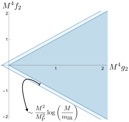
Figure 1: Schematic representation of our bounds: the weak gravity conjectures is satisfied at leading order (dark shaded region), but violations are still admissible at sub-leading order in $M/M_{\mathrm{P}}$ (light shaded region).

The purpose of this paper is to explore the use of dispersion relations and positivity bounds in the Einstein–Maxwell EFT. Our main conclusions are

• Using the generalized optical theorem, we bound quantities without manifestly positive spectral densities. This allows us to derive positivity bounds involving all three independent amplitudes $f\sim\mathcal{M}^{++++}$, $g\sim\mathcal{M}^{++--}$ and $h\sim\mathcal{M}^{+++-}$.

• In the limit where gravity decouples, it is easy to prove the WGC inequalities (2) by expanding in the forward limit. This is consistent with previous work Hamada:2018dde ; Bellazzini:2019xts , where it was shown that the WGC immediately follows if the graviton pole is discarded.

• We show how to derive corrections to the $M_{\mathrm{P}}\to\infty$ limit. The strongest possible bounds with our approach allow for a violation of the WGC: introducing the notation $16\alpha_{1,2}=g_{2}\pm f_{2}$, the WGC would require $g_{2}\geqslant|f_{2}|\geqslant 0$. Instead we find

  $$g_{2}>-\frac{c_{1}}{M^{2}M_{\mathrm{P}}^{2}}\log(M/m_{\mathrm{IR}})\,,$$ (12)

  where we give upper bounds on the $O(1)$ constant $c_{1}<24.2571$. A schematic representation of our bounds in the $(g_{2},f_{2})$ plane is shown in figure 1. The WGC appears to be satisfied at leading order in $M/M_{\textrm{P}}$, but zooming in on the boundaries of the allowed region unveils a region where it is violated. The size of the violation is suppressed by $(M/M_{\textrm{P}})^{2}$ but enhanced by the logarithm of an infrared cut-off.

This paper is organized as follows: In section 2, we review the fundamentals of $2\to 2$ photon scattering and the assumptions we use. Among these are (1) weak coupling: the requirement that loops are suppressed in the EFT, and (2) Regge boundedness: the requirement that, at fixed $u$, the amplitude grows slower than $s^{2}$ at large $|s|$. We also describe the approach to scattering non-identical states known as the “generalized optical theorem,” and show how it improves the bounds obtained in the limit without gravity.

In section 3, we consider the problem of bounding the EFT coefficients in the presence of gravity. We derive a number of improved sum rules and use them to bound the four-derivative coefficients. Some explicit examples of functionals which yield these bounds are given. We end the section with a discussion on the relevance of our bounds to the WGC.

2 Bounding Photon Scattering

Let us first review the technical ingredients we will need in order to derive bounds. The goal will be to apply dispersion relations to $2\to 2$ scattering amplitudes of photons. The result will be a set of sum rules which depend on Mandelstam invariants $s$ and $u$. Semi-definite programming may then be used to derive optimal constraints on EFT coefficients from these sum rules. This numerical approach to deriving EFT constraints was pioneered in Caron-Huot:2020cmc , and generalized to handle the graviton pole in Caron-Huot:2021rmr .

At the heart of this method is the $S$-matrix, which maps ingoing states to outgoing states. For the four-particle amplitudes considered here, this amounts to

$${}_{\text{out}}\left\langle\psi_{3}\psi_{4}\middle|\psi_{1}\psi_{2}\right\rangle_{\text{in}}={}_{\text{free}}\left\langle\psi_{3}\psi_{4}\middle|S\middle|\psi_{1}\psi_{2}\right\rangle_{\text{free}}\,,$$ (13)

for particles $\psi_{1}$, $\psi_{2}$, $\psi_{3}$, and $\psi_{4}$. The $S$-matrix can be split into the identity operator and the interacting part as

$$S={\mathds{1}}+iT\,.$$ (14)

For the four-particle amplitude, we consider the external states to be two-particle center-of-mass plane waves. We will be concerned with the scattering of photons, hence the amplitudes will be depend on the helicities of the external particles, $\mathcal{M}^{\lambda_{1}\lambda_{2}\lambda_{3}\lambda_{4}}$, where $\lambda_{i}=\pm$ denote states of circular polarization. We define the amplitude by

$$\left\langle p_{f},\theta,\phi,\lambda_{3},\lambda_{4}\middle|T\middle|p_{i},0,0,\lambda_{1},\lambda_{2}\right\rangle=(2\pi)^{4}\,\delta^{(4)}\left(\sum p_{i}^{\mu}\right)\,\mathcal{M}^{\lambda_{1}\lambda_{2}\lambda_{3}\lambda_{4}}(s,t,u)\,.$$ (15)

This describes two photons with helicities $\lambda_{1}$ and $\lambda_{2}$ coming in along the $z$-axis, and scattering to two photons with helicities $\lambda_{3}$ and $\lambda_{4}$, going in the direction $(\theta,\phi)$ and $(\pi-\theta,\pi+\phi)$. We shall use all-ingoing conventions in this paper. The dynamics are symmetric with respect to rotating $\phi$, so we will set it to $0$.

It will be convenient to package the individual helicity amplitudes into a matrix

$$\mathbf{M}=\begin{pmatrix}\mathcal{M}^{++--}&\mathcal{M}^{++-+}&\mathcal{M}^{+++-}&\mathcal{M}^{++++}\\ \mathcal{M}^{+---}&\mathcal{M}^{+--+}&\mathcal{M}^{+-+-}&\mathcal{M}^{+-++}\\ \mathcal{M}^{-+--}&\mathcal{M}^{-+-+}&\mathcal{M}^{-++-}&\mathcal{M}^{-+++}\\ \mathcal{M}^{----}&\mathcal{M}^{---+}&\mathcal{M}^{--+-}&\mathcal{M}^{--++}\end{pmatrix}\,.$$ (16)

Here we see 16 amplitudes, but in the scattering of identical indistinguishable particles, there are discrete symmetries which reduce the number of independent functions which these depend on. For our case, where all particles have spin 1, the amplitudes are related by

$$\mathcal{P}: \qquad\mathcal{A}^{\lambda_{1}\lambda_{2}\lambda_{3}\lambda_{4}}=\mathcal{A}^{-\lambda_{1}-\lambda_{2}-\lambda_{3}-\lambda_{4}}\,,$$ (17)

$$\mathcal{T}: \qquad\mathcal{A}^{\lambda_{1}\lambda_{2}\lambda_{3}\lambda_{4}}=\mathcal{A}^{-\lambda_{3}-\lambda_{4}-\lambda_{1}-\lambda_{2}}\,,$$ (18)

$$\mathcal{B}: \qquad\mathcal{A}^{\lambda_{1}\lambda_{2}\lambda_{3}\lambda_{4}}=\mathcal{A}^{\lambda_{2}\lambda_{1}\lambda_{4}\lambda_{3}}\,,$$ (19)

following from parity, time-reversal and boson exchange respectively.

In addition to the helicities, these amplitudes are functions of the momenta of the external particles, parametrized by the usual Mandelstam invariants, $s=-(p_{1}+p_{2})^{2}$, $t=-(p_{1}-p_{4})^{2}$, and $u=-(p_{1}-p_{3})^{2}$. The amplitudes are also related by crossing symmetry, which acts on their helicities and permutes the Mandelstam invariants (e.g. $\mathcal{M}^{++--}(s,t,u)=\mathcal{M}^{+-+-}(t,s,u)$, and by complex conjugation of the helicities which relates $\mathcal{M}^{-\lambda_{1}-\lambda_{2}-\lambda_{3}-\lambda_{4}}(s,t,u)=\mathcal{M}^{\lambda_{1}\lambda_{2}\lambda_{3}\lambda_{4}*}(s,t,u)\equiv(\mathcal{M}^{\lambda_{1}\lambda_{2}\lambda_{3}\lambda_{4}}(s^{*},t^{*},u^{*}))^{*}$.

Now let us count the number of independent amplitudes. In the most general situation, we only allow two symmetries $\mathcal{B}$ and $\mathcal{P}\mathcal{T}$. This reduces the number of independent functions from 16 to 7 (real) functions, which reduces to 5 after crossing symmetry:

$$\mathbf{M}=\begin{pmatrix}g(s|t,u)&h(s,t,u)&h(s,t,u)&f(s,t,u)\\ h^{*}(s,t,u)&g(t|s,u)&g(u|s,t)&h(s,t,u)\\ h^{*}(s,t,u)&g(u|s,t)&g(t|s,u)&h(s,t,u)\\ f^{*}(s,t,u)&h^{*}(s,t,u)&h^{*}(s,t,u)&g(s|t,u)\end{pmatrix}\,.$$ (20)

In this case, $g(s|t,u)$ is a real function with $t$-$u$ symmetry. $f(s,t,u)$ and $h(s,t,u)$ are complex functions, fully symmetric under any permutation of $s$-$t$-$u$. Their real and imaginary parts reflect the parity-even and parity-odd parts respectively. In the rest of this paper, we will restrict ourselves to parity-even interactions. In this case, $f^{*}(s,t,u)=f(s,t,u)$ and $h^{*}(s,t,u)=h(s,t,u)$. As a result, we are left with only three independent real functions, $f$, $g$, and $h$.

2.1 Dispersion relations

Dispersion relations are a standard technique for deriving positivity bounds. The typical strategy is the following: Consider an amplitude $\mathcal{M}(s,u)$ which obeys the Froissart bound

$$\lim_{s\to\infty}\frac{\mathcal{M}(s,u)}{s^{2}}=0\,,$$ (21)

at fixed $u$ in the physical region where $u<0$. This behavior has been demonstrated for gapped systems Froissart:1961ux ; Martin:1965jj , however for scattering of massless particles its status is less clear – see Chowdhury:2019kaq for an interesting recent discussion, and Haring:2022cyf for a proof of the required property for scalar amplitudes in $d>4$. In this paper, we will take (21) as an assumption.

Equation (21) implies that the following doubly-subtracted contour integral vanishes,

$$\int_{\infty}\frac{ds^{\prime}}{2\pi i}\frac{\mathcal{M}(s^{\prime},u)}{(s^{\prime}-s)s^{\prime}(s^{\prime}+u)}=0\,.$$ (22)

If the amplitude is analytic in the upper half $s$-plane, which follows from causality, then the contour can be deformed towards the real-$s$ axis, defining the amplitude on the lower-half plane via $\mathcal{M}(s,u)\equiv\mathcal{M}(s^{*},u^{*})^{*}$. Then there are two contributions to the integral, which must therefore cancel: one contribution from three simple poles, and one contribution from the discontinuity across two cuts along the real axis, see figure 2. In a parity-respecting theory, the discontinuity picks up the imaginary part of the amplitude, and we get

$$\begin{split}0\ &=\ \left(\operatorname*{res}_{s^{\prime}=s}+\operatorname*{res}_{s^{\prime}=0}+\operatorname*{res}_{s^{\prime}=-u}\right)\frac{\mathcal{M}(s^{\prime},u)}{(s-s^{\prime})s^{\prime}(s^{\prime}+u)}\\ &\ \quad-\int_{M^{2}}^{\infty}\frac{ds^{\prime}}{\pi}\operatorname*{Im}\left[\frac{\mathcal{M}(s^{\prime},u)}{(s-s^{\prime})s^{\prime}(s^{\prime}+u)}\right]-\int_{-\infty}^{-M^{2}-u}\frac{ds^{\prime}}{\pi}\operatorname*{Im}\left[\frac{\mathcal{M}(s^{\prime},u)}{(s-s^{\prime})s^{\prime}(s^{\prime}+u)}\right]\,.\end{split}$$ (23)

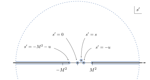
Figure 2: The starting point for our dispersive argument is the dashed contour at infinity in the $s^{\prime}$ plane. It is deformed inwards to pick up contributions from three low-energy poles and two infinite cuts.

The strategy we will follow below is to parametrize the amplitude in the top line of (23) using the EFT, where it is given as a sum of undetermined coefficients. The amplitude in the bottom line will be parametrized using the partial wave expansion. Unitarity implies that the partial wave densities are positive (or, more generally, form positive definite matrices). This will allow us to convert (23) into an equation of the form $\mathbf{L}=\mathbf{H}$, where $\mathbf{L}$ and $\mathbf{H}$ are the low- and high-energy results of the dispersion integral and will be defined below.

2.2 Low-energy: EFT expansion

For parity-respecting theories, the scattering of photons is described by three independent real functions, $f$, $g$, and $h$. At low energies, these functions are approximated by an effective field theory, i.e. (1), and they may be expanded in powers of the Mandelstam invariants. The functions $f(s,t,u)$ and $h(s,t,u)$ are individually $s$-$t$-$u$ symmetric, while $g(s|t,u)$ is $t$-$u$ symmetric. These functions have expansions in small values of the Mandelstam invariants

$$\begin{split}f(s,t,u)&=10\frac{\beta^{2}}{M_{\mathrm{P}}^{2}}\,stu+f_{2}\,(s^{2}+t^{2}+u^{2})+f_{3}\,stu+f_{4}\,(s^{2}+t^{2}+u^{2})^{2}+\ldots,\\ g(s|t,u)&=\frac{1}{M_{\mathrm{P}}^{2}}\frac{s^{3}}{tu}+\frac{\beta^{2}}{M_{\mathrm{P}}^{2}}\!\left(\!4stu-\frac{2}{3}s^{3}\right)+g_{2}s^{2}+g_{3}s^{3}+g_{4,1}s^{4}+g_{4,2}s^{2}(s^{2}+t^{2}+u^{2})+\ldots,\\ h(s,t,u)&=\frac{\beta}{M_{\mathrm{P}}^{2}}(s^{2}+t^{2}+u^{2})+h_{3}\,stu+h_{4}\,(s^{2}+t^{2}+u^{2})^{2}+\ldots.\end{split}$$ (24)

By a direct computation, we note that the first terms in these expressions agree with the action (1) upon identifying $16\alpha_{1}=g_{2}+f_{2}$ and $16\alpha_{2}=g_{2}-f_{2}$. The remaining parametrization allows for all possible terms consistent with the mentioned symmetries, and the assumption that contact interactions give a contribution to $g(s|t,u)$ proportional to $s^{2}$.

Gravity decouples in the $M_{\mathrm{P}}\to\infty$ limit, and the terms that involve graviton propagators go to zero in this limit. Let us comment on the terms with $\beta$, which are a little special: $\beta$ arises from the Feynman diagrams with a single or double insertion of the operator $F_{\mu\nu}F_{\rho\sigma}W^{\mu\nu\rho\sigma}$, together with a graviton propagator in the diagram. From the way we have written it, it is clear that these terms vanish in the $M_{\mathrm{P}}\to\infty$ limit. But one might ask why not also include an independent $h_{2}$ term, i.e. a term $h_{2}\,(s^{2}+t^{2}+u^{2})$ in $h(s,t,u)$. In fact, we shall see that forward-limit sum rules, which are applicable in the limit where gravity has decoupled, preclude the existence of any such term (and in fact also show that $h_{4}=0$). The $h_{2}$-type interaction must shut off in that limit.

In terms of the matrix of amplitudes, we will introduce $\mathbf{L}$, the low-energy matrix, by

$$\mathbf{L}\equiv\left(\operatorname*{res}_{s^{\prime}=s}+\operatorname*{res}_{s^{\prime}=0}+\operatorname*{res}_{s^{\prime}=-u}\right)\frac{\mathbf{M}(s^{\prime},u)}{(s^{\prime}-s)s^{\prime}(s^{\prime}+u)}\,.$$ (25)

Using “prime” to denote this sum over residues, this can be written as

$$\mathbf{L}=\begin{pmatrix}g^{\prime}(s|t,u)&h^{\prime}(s,t,u)&h^{\prime}(s,t,u)&f^{\prime}(s,t,u)\\ h^{\prime}(s,t,u)&g^{\prime}(t|s,u)&g^{\prime}(u|s,t)&h^{\prime}(s,t,u)\\ h^{\prime}(s,t,u)&g^{\prime}(u|s,t)&g^{\prime}(t|s,u)&h^{\prime}(s,t,u)\\ f^{\prime}(s,t,u)&h^{\prime}(s,t,u)&h^{\prime}(s,t,u)&g^{\prime}(s|t,u)\end{pmatrix}\,,$$ (26)

where

$$\begin{split}f^{\prime}(s,t,u)\ &=\ 2f_{2}-\left(f_{3}+10\frac{\beta^{2}}{M_{\mathrm{P}}^{2}}\right)\,u+4f_{4}(s^{2}+su+2u^{2})+\ldots,\\ g^{\prime}(s|t,u)\ &=\ -\frac{1}{M_{\mathrm{P}}^{2}u}+g_{2}+g_{3}(s-u)-\frac{2}{3}\frac{\beta^{2}}{M_{\mathrm{P}}^{2}}\,(s+5u)\\ &\qquad\qquad+g_{4,1}(s^{2}-su+u^{2})+2g_{4,2}(s^{2}+u^{2})+\ldots,\\ g^{\prime}(t|s,u)\ &=\ -\frac{1}{M_{\mathrm{P}}^{2}u}+g_{2}-g_{3}(s+2u)+\frac{2}{3}\frac{\beta^{2}}{M_{\mathrm{P}}^{2}}\,(s-4u)\\ &\qquad\qquad+g_{4,1}\,(s^{2}+3su+3u^{2})+g_{4,2}\,(2s^{2}+4su+4u^{2})+\ldots,\\ g^{\prime}(u|s,t)\ &=\ -4\frac{\beta^{2}}{M_{\mathrm{P}}^{2}}\,u+2g_{4,2}\,u^{2}+\ldots,\\ h^{\prime}(s,t,u)\ &=\ 2\frac{\beta}{M_{\mathrm{P}}^{2}}-h_{3}u+4h_{4}(s^{2}+su+2u^{2})+\ldots.\end{split}$$ (27)

The low-energy part is entirely determined by these functions $f^{\prime}$, $g^{\prime}$, and $h^{\prime}$.

2.3 High-energy: partial waves and unitarity

Now we turn to the high-energy part of the dispersion relation, defined by

$$\begin{split}\mathbf{H}&=\int_{-\infty}^{-u-M^{2}}\,\frac{ds^{\prime}}{\pi}\,\operatorname*{Im}{\left[\frac{\mathbf{M}(s^{\prime},u)}{(s^{\prime}-s)s^{\prime}(s^{\prime}+u)}\right]}+\int_{M^{2}}^{\infty}\,\frac{ds^{\prime}}{\pi}\,\operatorname*{Im}{\left[\frac{\mathbf{M}(s^{\prime},u)}{(s^{\prime}-s)s^{\prime}(s^{\prime}+u)}\right]}\,\\ &\qquad=\int_{M^{2}}^{\infty}\,\frac{ds^{\prime}}{\pi}\,\operatorname*{Im}{\left[\frac{\mathbf{M}(s^{\prime},u)}{(s^{\prime}-s)s^{\prime}(s^{\prime}+u)}+\frac{\mathbf{M}(-s^{\prime}-u,u)}{(s+s^{\prime}+u)s^{\prime}(s^{\prime}+u)}\right]}\,.\end{split}$$ (28)

The amplitudes $\mathbf{M}(s^{\prime},u)$ and $\mathbf{M}(-s^{\prime}-u,u)$ can be related by crossing, and we will use this fact to derive the exact form of the sum rules.

At high-energies, i.e. above the scale $M$, the EFT no longer applies, and we are forced to be more agnostic about the form of the amplitude. However the symmetries alone strongly constrain the possible form the amplitude can take. This motivates the use of the partial wave expansion. For spinning particles in four dimensions, this takes the form Jacob:1959at

$$M^{IJ}=16\pi\sum_{\ell}(2\ell+1)A_{\ell}^{IJ}(s)d^{\ell}_{\lambda_{I}\lambda_{J}}(\theta)\,.$$ (29)

Here $I$ and $J$ label the rows and columns of the matrix, or equivalently pairs of helicities. The partial wave densities $A^{IJ}_{\ell}(s)$ are given by

$$A^{\lambda_{1}\lambda_{2}\lambda_{3}\lambda_{4}}_{\ell}(s)=\left\langle s,\ell,\lambda_{3},\lambda_{4}\middle|T\middle|s,\ell,\lambda_{1},\lambda_{2}\right\rangle\,,$$ (30)

where $|s\ell\lambda_{1}\lambda_{2}\rangle$ refers to a two-particle state with definite angular momentum $\ell$ and energy $\sqrt{s}$. The Wigner $d$ functions $d_{\lambda_{I}\lambda_{J}}$ are functions of $\lambda_{I}=\lambda_{1}(I)-\lambda_{2}(I)$, $\lambda_{J}=\lambda_{4}(J)-\lambda_{3}(J)$, and the scattering angle $\theta=\arccos\left(1+\frac{2u}{m^{2}}\right)$. The set of allowed values of the spin $\ell$ of exchanged states depends on the external helicities. As we will see below, for $f(s,t,u)$ and $g(s|t,u)$ we have $\ell=0,2,4,\ldots$, for $g(t|s,u)$ and $g(u|s,t)$, $\ell=2,3,4,\ldots$, and for $h(s,t,u)$, $\ell=2,4,6,\ldots$.

Now we define the spectral densities $\rho^{\lambda_{1}\lambda_{2}\lambda_{3}\lambda_{4}}_{\ell}(s)=\operatorname*{Im}A^{\lambda_{1}\lambda_{2}\lambda_{3}\lambda_{4}}_{\ell}(s)$. Using the partial wave expansion in the integral, and combining the right-hand and left-hand cuts using crossing symmetry, we find an expression for the components of $\mathbf{H}$. From here on, we will use $s^{\prime}=m^{2}$. Then we have

$$\begin{split}\mathbf{H}^{\lambda_{1}\lambda_{2}\lambda_{3}\lambda_{4}}&=\int_{M^{2}}^{\infty}\frac{dm^{2}}{m^{2}}\sum_{\ell}16(2\ell+1)\bigg{(}\rho_{\ell}^{\lambda_{1}\lambda_{2}\lambda_{3}\lambda_{4}}(m^{2})\frac{d_{\lambda_{1}-\lambda_{2},\lambda_{4}-\lambda_{3}}^{\ell}(\theta)}{(m^{2}-s)(m^{2}+u)}\\ &\quad\qquad\qquad\qquad\qquad\qquad+\rho_{\ell}^{\lambda_{1}\lambda_{4}\lambda_{3}\lambda_{2}}(m^{2})\frac{d^{\ell}_{\lambda_{1}-\lambda_{4},\lambda_{2}-\lambda_{3}}(\theta)}{(m^{2}+u)(m^{2}+s+u)}\bigg{)}\,.\end{split}$$ (31)

For convenience, let us denote the integrand by $h^{IJ}$, so that

$$H^{IJ}=\int_{M^{2}}^{\infty}\frac{dm^{2}}{m^{2}}\sum_{\ell}h^{IJ}\,.$$ (32)

2.3.1 Positivity from unitarity

Having defined $h^{IJ}$, we shall now write it in a way that separates the dynamical and kinematical content of the high-energy amplitude. The aim is to do it in such a way that it makes the positivity conditions manifest. The key to finding positivity condition is to invoke unitarity, which implies that

$$S^{\dagger}S=1\quad\implies\quad 2\operatorname*{Im}T=T^{\dagger}T\,.$$ (33)

Contracting the second equation with external states of definite helicity and angular momentum $\ell$ gives

$$\operatorname*{Im}A^{IJ}_{\ell}(s)=\frac{1}{2}\langle s,\ell,\lambda_{3},\lambda_{4}|T^{\dagger}T|s,\ell,\lambda_{1},\lambda_{2}\rangle=\frac{1}{2}\sum_{X}\langle s,\ell,\lambda_{3},\lambda_{4}|T^{\dagger}|X\,\ell\rangle\langle X\,\ell|T|s,\ell,\lambda_{1},\lambda_{2}\rangle\,,$$ (34)

where we have inserted a complete set of intermediate states of spin $\ell$, labeled by $X$, which accounts for all other labeling of the state. If we define

$$c^{\lambda_{i}\lambda_{j}}_{\ell,X}(s)=\sqrt{8(2\ell+1)}\langle X\ell|T|s,\ell,\lambda_{i},\lambda_{j}\rangle\,,$$ (35)

and use $\rho_{\ell}=\operatorname*{Im}A_{\ell}$, the result is

$$16(2\ell+1)\rho_{\ell}^{\lambda_{1}\lambda_{2}\lambda_{3}\lambda_{4}}(s)=\sum_{X}c^{\lambda_{1}\lambda_{2}}_{\ell,X}(s)\left(c^{-\lambda_{3}-\lambda_{4}}_{\ell,X}(s)\right)^{*}\,.$$ (36)

From this result, sometimes called the generalized optical theorem (e.g. Du:2021byy ), we can see that $\rho^{IJ}_{\ell}(s)$ is a positive definite Hermitian matrix. In what follows, we shall use the positivity of $\rho^{IJ}_{\ell}(s)$ to show that specific linear combinations of the high-energy part of the dispersion relation are positive. Specifically, they will be constructed by acting on $\mathbf{H}$ by certain linear functionals which will involve contracting $\mathbf{H}^{IJ}$ with vectors $v^{I}$, and taking various integrals over $u$. To make this concrete, let us start by rewriting $h^{IJ}$ as

$$h^{IJ}(\ell,m^{2},s,u)=\sum_{Q}\sum_{X}\boldsymbol{c}_{\ell,X}^{\dagger}(m^{2})V^{IJ}_{Q}(\ell,m^{2},s,u)\boldsymbol{c}_{\ell,X}(m^{2})\,,$$ (37)

where for generality we consider a vector $\boldsymbol{c}_{\ell,X}$ and a matrix $V_{Q}^{IJ}$. The $V^{IJ}_{Q}$ may be determined from (31) and are given in explicit form in appendix A. The purpose of defining $h^{IJ}$ this way is that it makes the positivity constraints easier to deal with. This follows from the fact that for a real-valued symmetric matrix $V$, the condition $V\succcurlyeq 0$ implies that $\boldsymbol{c}^{\dagger}V\boldsymbol{c}\geq 0$ for all complex vectors $\boldsymbol{c}$. Since all the dynamical information of the high-energy amplitude is contained in the vectors $\boldsymbol{c}$, we can analyze its positivity without making any further assumptions than those following from analyticity, unitarity and symmetry. Below we shall see how to construct sum rules by contracting (37) with vectors different vectors $\boldsymbol{v}$, and derive positivity constraints by applying linear functionals on such sum rules.

In (37), the sum over $Q$ represents a sum over “selection sectors” – defined by the parity $P_{X}$ and spin $\ell_{X}$ of the exchanged state. Invariance under parity and boson exchange imply

$$c_{\ell,X}^{\lambda_{1}\lambda_{2}} =P_{X}c_{\ell,X}^{-\lambda_{2}-\lambda_{1}}\,,$$ (38)

$$c_{\ell,X}^{\lambda_{1}\lambda_{2}} =(-1)^{\ell}c_{\ell,X}^{\lambda_{2}\lambda_{1}}\,.$$ (39)

From this, we can see that $c^{++}=c^{--}=0$ for odd spins, and $c^{+-}=c^{-+}=0$ for odd parity. Thus, we have that $Q$ ranges over the following sectors:

• Spin zero and parity-even, denoted $Q=0$. We have $c^{0}_{0,X}=(c_{0,X}^{++})^{*}$, and $V_{0}^{IJ}$ is a number for any fixed $I,J$.

• Even spin $\ell=2,4,\ldots$ and parity-even, denoted $Q=+$. We have $\boldsymbol{c}^{+}_{\ell,X}=(c_{\ell,X}^{++},c^{+-}_{\ell,X})^{\dagger}$ and $V_{+}^{IJ}$ is a $2\times 2$ matrix for any fixed $I,J$.

• Even spin $\ell=0,2,4,\ldots$ and parity-odd, denoted $Q=-$. We have $c^{-}_{\ell,X}=(c_{\ell,X}^{++})^{*}$, and $V_{-}^{IJ}$ is a number for any fixed $I,J$.

• Odd spin $\ell=3,5,\ldots$ and parity-even, denoted $Q=o$. We have $c^{o}_{\ell,X}=(c_{\ell,X}^{+-})^{*}$, and $V_{o}^{IJ}$ is a number for any fixed $I,J$.

There are no parity-odd exchanges for odd spin. With these considerations at hand, we are able to write the matrix entries of the high-energy integrand $\mathbf{h}$ as

$$h^{IJ}(m^{2},s,u)= \sum_{X}|c_{0,X}^{0}|^{2}V_{0}^{IJ}(m^{2},s,u)+\sum_{\ell=2,4,\ldots}\sum_{X}\sum_{a,b=1}^{2}(c_{\ell,X}^{+})^{a}({c_{\ell,X}^{+}}^{*})^{b}(V^{IJ}_{+})^{ab}(\ell,m^{2},s,u)$$

$$+\sum_{\ell=0,2,\ldots}\sum_{X}|c^{-}_{\ell,X}|^{2}V^{IJ}_{-}(\ell,m^{2},s,u)+\sum_{\ell=3,5,\ldots}\sum_{X}|c^{o}_{\ell,X}|^{2}V_{o}^{IJ}(\ell,m^{2},s,u)\,.$$ (40)

2.4 Sum rules

We may now express the result of our dispersive arguments in the form

$$\mathbf{L}=\mathbf{H}\,,$$ (41)

where $\mathbf{L}$ and $\mathbf{H}$, as defined above, are matrices of functions of $s$ and $u$. To proceed we will first contract the matrices with real vectors $v^{I}$, which will lead to

$$v^{I}L^{IJ}v^{J}=v^{I}H^{IJ}v^{J}\,.$$ (42)

The left and right sides of this equation are both functions of $s$ and $u$. From here, we make use of two basic ways to derive sum rules:

1. Choose powers $s^{p}u^{q}$ and look at

   $$\left.\boldsymbol{v}^{T}\mathbf{L}\boldsymbol{v}\right|_{s^{p}u^{q}}=\left.\boldsymbol{v}^{T}\mathbf{H}\boldsymbol{v}\right|_{s^{p}u^{q}}\,.$$ (43)

2. Choose the power $s^{0}$ and a function $\phi(p)=\phi(\sqrt{-u})$

   $$\int_{0}^{M}dp\,\phi(p)\left.\boldsymbol{v}^{T}\mathbf{L}\boldsymbol{v}\right|_{s^{0},u=-p^{2}}=\int_{0}^{M}dp\,\phi(p)\left.\boldsymbol{v}^{T}\mathbf{H}\boldsymbol{v}\right|_{s^{0},u=-p^{2}}\,.$$ (44)

We refer to the first type of sum rules as “forward-limit sum rules” because they essentially amount to a series expansion around $u=0$. This means that they are not valid in the presence of a $1/u$ graviton pole. The second type we shall call “integral sum rules.” These are more general: they include the forward-limit sum rules when $\phi(u)$ has a $\delta(u)$ factor.

In practice, we shall consider linear combinations of such sum rules. The primary reason to do this is to derive “improved sum rules,” where the low-energy part only depends on a finite number of EFT coefficients. We shall show in detail how these are constructed below. A general linear combination of rules can be constructed from a linear combination of sum rules formed from different vectors $\boldsymbol{v}_{i}$. The practical algorithm will therefore be

If $$\forall Q,\ \forall\ell\in Q,\ \forall m^{2}\geqslant M^{2}$$

$$\sum_{i}\left.v_{i}^{I}V^{IJ}_{Q}(\ell,m^{2},s,u)v_{i}^{J}\right|_{s^{p_{i}}u^{q_{i}}}+\sum_{i}\int_{0}^{M}dp\,\phi_{i}(p)\left.v_{i}^{I}V^{IJ}_{Q}(\ell,m^{2},s,u)v_{i}^{J}\right|_{s^{0},u=-p^{2}}\succcurlyeq 0,$$ (45)

Then $$\sum_{i}\left.\boldsymbol{v}_{i}^{I}L^{IJ}\boldsymbol{v}^{J}_{i}\right|_{s^{p_{i}}u^{q_{i}}}+\sum\int_{0}^{M}dp\,\phi_{i}(p)\left.\boldsymbol{v}_{i}^{I}L^{IJ}\boldsymbol{v}^{J}_{i}\right|_{s^{0},u=-p^{2}}\geqslant 0\,.$$ (46)

The argument is as follows. It follows from (40) that if the condition (45) is true, then

$$\sum_{i}\left.v_{i}^{I}h^{IJ}v_{i}^{J}\right|_{s^{p_{i}}u^{q_{i}}}+\sum_{i}\int_{0}^{M}dp\,\left.\phi_{i}(p)v_{i}^{I}h^{IJ}v_{i}^{J}\right|_{s^{0},u=-p^{2}}\geqslant 0\,.$$ (47)

Then by (32), the high-energy part of the dispersion relation is positive. This implies that the low-energy part must also be positive, implying the positivity in (46).

To connect with the numerical bootstrap philosophy, we will think of the (weighted) sum over different choices of $i$ in the argument above as acting on a set of sum rules with a linear functional $\Lambda$. Specifically, on matrix-valued functions $f^{IJ}(s,u,m^{2})$

$$\Lambda[f^{IJ}]=\sum_{i}\left.v_{i}^{I}f^{IJ}(m^{2},s,u)v_{i}^{J}\right|_{s^{p_{i}}u^{q_{i}}}+\sum_{i}\int_{0}^{M}dp\left.\phi_{i}(p)v_{i}^{I}f^{IJ}(m^{2},s,-p^{2})v_{i}^{J}\right|_{s^{0}}\,.$$ (48)

Then the algorithm can be reformulated in terms of searching for optimal functionals, a problem that can be implemented as a semi-definite program. Specifically,

$$\text{If}\qquad\Lambda[V_{0}^{IJ}] \geqslant 0\quad\text{for all }m^{2}\geqslant M^{2}\,$$

$$\Lambda[V_{+}^{IJ}(\ell)] \succcurlyeq 0\quad\text{for all }m^{2}\geqslant M^{2},\ \ell=2,4,6,\ldots\,,$$

$$\Lambda[V_{-}^{IJ}(\ell)] \geqslant 0\quad\text{for all }m^{2}\geqslant M^{2},\ \ell=0,2,4,\ldots\,,$$ (49)

$$\Lambda[V_{o}^{IJ}(\ell)] \geqslant 0\quad\text{for all }m^{2}\geqslant M^{2},\ \ell=3,5,7,\ldots\,,$$

$$\text{Then}\qquad\Lambda[L^{IJ}] \geqslant 0\,.$$ (50)

2.4.1 Null constraints

Another important part of the numerical method of this paper is the addition of null constraints, first introduced in Tolley:2020gtv ; Caron-Huot:2020cmc . The are equations that arise when a single EFT coefficient can be written in terms of the high-energy expansion in two different ways. As such, they take the form of constraints only on the high-energy data. Including them in the numerics significantly improves the possible bounds. The use of null constraints for photon scattering in the forward limit was explained in Henriksson:2021ymi : in practice one expands the dispersion relations as in (43), with $p$ sufficiently large to kill the graviton pole, and equates high-energy expansions leading to the same low energy expression. In this paper, however, we find more null constraints than in our previous work. Consider the sum rules derived from the “$g$-type” amplitudes only: $g(s|t,u)$, $g(t|s,u)$ and $g(u|s,t)$. Each of these amplitudes enters a dispersion relation, not manifestly positive. In Henriksson:2021ymi , only $s$-$t$ symmetric combinations were considered, effectively reducing the number of amplitudes to consider to two: $g(s|t,u)+g(t|s,u)$ and $g(u|s,t)$.

Table 1: Number of sum rules and null constraints constructed from the $g$-type amplitudes only. The coefficients $\tilde{g}_{p,q}$ are not important for our discussion.

Order	Sum rules	Null constraints: Henriksson:2021ymi	Null constraints: this work
$\frac{1}{m^{4}}$	1: $g_{2}$	0	0
$\frac{1}{m^{6}}$	1: $g_{3}$	0	1
$\frac{1}{m^{8}}$	2: $g_{4,1}$, $g_{4,2}$	1	2
$\frac{1}{m^{10}}$	2: $\tilde{g}_{3,0}$, $\tilde{g}_{3,1}$	1	3
$\frac{1}{m^{12}}$	3: $\tilde{g}_{4,0}$, $\tilde{g}_{4,1}$, $\tilde{g}_{4,2}$	1	4

The counting of null constraints is given in table 1. When considering only $g$-type sum rules, this leads to stronger constraints than the previous work. Moreover, we now have sum rules and null constraints involving the “$h$-type” amplitudes.

Another addition to the previous work is the null constraints of the form of integral sum rules. We will return to them in section 3.

2.5 Bounds without gravity

The rest of this section will be devoted to applying the methodology laid out above to the case where $M_{\mathrm{P}}\to\infty$. In this limit, gravity decouples and the graviton pole vanishes. This means that we may apply forward-limit sum rules with as few as two subtractions, i.e. $p\geqslant 0$ in (43). After reviewing these sum rules in more depth, we present a number of bounds derived from them. Among other things, we show how this immediately implies the WGC inequalities (2). This is consistent with the known fact that the WGC is directly provable from forward-limit bounds if the graviton pole is ignored Bellazzini:2019xts .

The problem of bounding $2\to 2$ photon amplitudes in the absence of gravity was addressed using a less general method in Henriksson:2021ymi . As such, we also include a discussion of the difference between the results obtained here and the results of that paper. We see that they are significantly stronger and we are also able to bound coefficients, such as $h_{3}$, which remain unconstrained in Henriksson:2021ymi .

2.5.1 Forward-limit sum rules

Recall that the sum rules take the form $\mathbf{L}=\mathbf{H}$, with components

$$L^{IJ}\ =\ \int_{M^{2}}^{\infty}\frac{dm^{2}}{m^{2}}\sum_{Q}\sum_{\ell}\sum_{X}\boldsymbol{c}_{\ell,X}^{\dagger}V_{Q}^{IJ}(\ell,m^{2},s,u)\boldsymbol{c}_{\ell,X}\,.$$ (51)

Contracting with a vector $\boldsymbol{v}$ and writing out the sum over $Q\in\{0,+,-,o\}$ explicitly gives

$$\boldsymbol{v}^{T}\mathbf{L}\boldsymbol{v}|_{s^{p}u^{q}}= \int_{M^{2}}^{\infty}\frac{dm^{2}}{m^{2}}\bigg{(}\sum_{X}|c_{X,0}^{0}|^{2}v^{I}V^{IJ}_{0}v^{J}+\sum_{\ell=2,4,\ldots}\sum_{X}\sum_{a,b=1}^{2}(c_{\ell,X}^{+})^{a}({c_{\ell,X}^{+}}^{*})^{b}v^{I}(V_{+}^{IJ})^{ab}v^{J}$$

$$+\sum_{\ell=0,2,\ldots}\sum_{X}|c^{-}_{\ell,X}|^{2}v^{I}V_{-}^{IJ}v^{J}+\sum_{\ell=3,5,\ldots}\sum_{X}|c^{o}_{\ell,X}|^{2}v^{I}V_{o}^{IJ}v^{J}\bigg{)}\,.$$ (52)

Positivity of $\boldsymbol{g_{2}}$

Let us illustrate this with a simple example. If we choose $\boldsymbol{v}=(1,0,0,0)^{T}$ then we find the low-energy part

$$\boldsymbol{v}^{T}\mathbf{L}\boldsymbol{v}=g^{\prime}(s|t,u)=\ g_{2}+g_{3}(s-u)+g_{4,1}(s^{2}-su+u^{2})+g_{4,2}(2s^{2}+2u^{2})+\ldots.$$ (53)

Consider the lowest-order sum rule by specifying $p=0$, $q=0$. This picks out $\left.\boldsymbol{v}^{T}\mathbf{L}\boldsymbol{v}\right|_{s^{0}u^{0}}=g_{2}$. For the high-enery part, we use the explicit formulas in appendix A. For our choice of $\boldsymbol{v}$ we get

$$\begin{split}v^{I}V^{IJ}_{0}v^{J}\ &=\ \frac{1}{(m^{2}-s)(m^{2}+u)}\,,\\ v^{I}V^{IJ}_{+}v^{J}\ &=\ \begin{pmatrix}\frac{d^{\ell}_{0,0}(\theta)}{(m^{2}-s)(m^{2}+u)}&0\\ 0&\frac{d^{\ell}_{2,2}(\theta)}{(m^{2}+u)(m^{2}+s+u)}\end{pmatrix}\,,\\ v^{I}V^{IJ}_{-}v^{J}\ &=\ \frac{d^{\ell}_{0,0}(\theta)}{(m^{2}-s)(m^{2}+u)}\,,\\ v^{I}V^{IJ}_{o}v^{J}\ &=\ \frac{d^{\ell}_{2,2}(\theta)}{(m^{2}+u)(m^{2}+s+u)}\,,\end{split}$$ (54)

where $\theta=1+\frac{2u}{s}$ is the scattering angle. Now the forward limit $u\to 0$ imples $\theta\to 0$, in which case $d^{\ell}_{0,0}(\theta)\to 1$ and $d^{\ell}_{2,2}(\theta)\to 1$. So we find that $\left.v^{I}V^{IJ}_{Q}v^{J}\right|_{s^{0}u^{0}}=m^{-4}$ for all of the sectors (except $\left.v^{I}V^{IJ}_{+}v^{J}\right|_{s^{0}u^{0}}=m^{-4}\mathbb{I}_{2}$). The result is a sum rules for $g_{2}$,

$$g_{2}= \int_{M^{2}}^{\infty}\frac{dm^{2}}{m^{6}}\bigg{(}\sum_{X}|c_{0,X}^{0}|^{2}+\!\!\sum_{\ell=2,4,\ldots}\!\sum_{X}\sum_{a=1}^{2}|(c_{\ell,X}^{+})^{a}|^{2}+\!\!\sum_{\ell=0,2,\ldots}\!\sum_{X}|c^{-}_{\ell,X}|^{2}+\!\!\sum_{\ell=3,5,\ldots}\!\sum_{X}|c^{o}_{\ell,X}|^{2}\bigg{)}.$$ (55)

It is clear that this is a sum over positive terms. Hence $g_{2}$ must be positive! This example, therefore, turns out to be a translation of known results Falkowski ; Bellazzini2016talk ; Henriksson:2021ymi into the language of this paper. Likewise, if one picks the power $s^{2k}u^{0}$, one finds a sum rule that implies positivity of the coefficient of $s^{2k+2}u^{0}$ in $g(s|t,u)$, in agreement with Arkani-Hamed:2020blm , see (166) in appendix A.

WGC bounds without gravity

Let us consider a slightly more complicated example, which will give us a very interesting result. Let us choose $\boldsymbol{v}^{T}=\frac{1}{4}(1,-1,-1,1)$, and again look at the leading (four-derivative) coefficients by specifying $p=q=0$. From the low-energy expansion, we can see that

$$\mathbf{L}|_{s^{2}u^{0}}=\begin{pmatrix}g_{2}&-2h_{2}&-2h_{2}&2f_{2}\\ -2h_{2}&g_{2}&0&-2h_{2}\\ -2h_{2}&0&g_{2}&-2h_{2}\\ 2f_{2}&-2h_{2}&-2h_{2}&g_{2}\end{pmatrix}\,,$$ (56)

so we find

$$\left.\boldsymbol{v}^{T}\mathbf{L}\boldsymbol{v}\right|_{s^{0}u^{0}}\ =\ g_{2}+f_{2}-4h_{2}\ =\ 4\left(4\alpha_{1}-\frac{\beta}{M_{\mathrm{P}}^{2}}\right)\,.$$ (57)

This is proportional to the exact combination that appears in the (electric) WGC bound in (2). Here we have defined $h_{2}=\beta/M_{\mathrm{P}}^{2}$. The reason is that $h_{2}=\beta/M_{\mathrm{P}}\to 0$ in the decoupling limit. However for the moment, we would like to be agnostic about the source of $h_{2}$ in the amplitude, and instead think of it as the nothing more than the coefficient of $s^{2}+t^{2}+u^{2}$ in the $h(s,t,u)$ amplitude.

Now let us look at the high-energy parts

$$\left.v^{I}V^{IJ}_{0}v^{J}\right|_{s^{0}u^{0}}\ =\ \frac{2}{m^{4}}\,,\quad \left.v^{I}V^{IJ}_{+}v^{J}\right|_{s^{0}u^{0}}\ =\ \frac{1}{m^{4}}\begin{pmatrix}2&0\\ 0&1\\ \end{pmatrix}\,,$$ (58)

$$\left.v^{I}V^{IJ}_{-}v^{J}\right|_{s^{0}u^{0}}\ =\ 0\,,\quad \left.v^{I}V^{IJ}_{o}v^{J}\right|_{s^{0}u^{0}}\ =\ \frac{1}{m^{4}}\,.$$ (59)

The consequence of this is a sum rule for the WGC combination:

$$\begin{split}&g_{2}+f_{2}-4h_{2}=\\ &\qquad\sum_{X}\int_{M^{2}}^{\infty}\frac{dm^{2}}{m^{6}}\bigg{(}2|c_{0,X}^{+}|^{2}+\sum_{\ell=2,4,\ldots}\left(2|(c_{\ell,X}^{+})^{1}|^{2}+|(c_{\ell,X}^{+})^{2}|^{2}\right)+\sum_{\ell=3,5,\ldots}|c^{o}_{\ell,X}|^{2}\bigg{)}\,.\end{split}$$ (60)

The result is a sum of squares, and must therefore be positive. This result is also known in the literature. It was pointed out in Hamada:2018dde ; Bellazzini:2019xts that these forward limit bounds directly imply the positivity of the WGC combination. Note also that we can easily obtain the magnetic and dyonic WGC inequalities by choosing instead choosing $\boldsymbol{v}=(1,1,1,1)^{T}$ and $\boldsymbol{v}=(1,1,1,-1)^{T}$, respectively.

Let us be clear that this does not prove the WGC: we are required to take the decoupling limit $M_{\mathrm{P}}\to\infty$ before we are allowed to use the forward-limit sum rules in the first place. As a result, it is sort of a silly example. Of course “gravity is the weakest force” in the limit where the strength of gravity goes to zero. Still, it serves to illustrate an important point: the bounds we can derive in the absence of gravity by expanding in the forward limit are stronger than the bounds available when the graviton pole is present. This shall be a major theme of section 3, where we will explore the bounds in the presence of gravity.

Vanishing of $\boldsymbol{h_{2}}$ without gravity

Let us define $h_{2}$ to be the term proportional to $s^{2}+t^{2}+u^{2}$ in the amplitude $h(s,t,u)$. The parametrization $h_{2}=\beta/M_{\mathrm{P}}^{2}$ used in (24) indicates that $h_{2}=0$ in the absence of gravity, and in fact it is easy to derive a sum rule that shows this fact. Consider for instance the entry $L^{12}|_{s^{0}}=2h_{2}-h_{3}u+\ldots$ in the low-energy amplitude. The corresponding entry $H^{12}|_{s^{0}}$ in the high-energy amplitude is in fact proportional to $u$, giving

$$2h_{2}-h_{3}u+\ldots=H^{12}|_{s^{0}}=0+O(u)\,,$$ (61)

which shows that $h_{2}=0$. Note that argument is not valid in the presence of gravity, since it requires expanding the twice-subtracted dispersion relation in the forward limit.

2.5.2 Numerical results

The strategy to get bounds is very similar to the one in Henriksson:2021ymi , but with two differences. The first one is that in this case we have a more general set of sum rules, which include the amplitude $\mathcal{M}^{+++-}$, too. Thus, we can now get bounds on the coefficients in the $h$ amplitude; the corresponding sum rules and null constraints are non-diagonal in $V_{+}^{IJ}$. For instance, the sum rule for $h_{3}$ reads

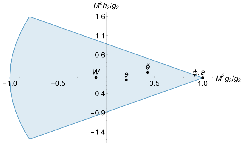
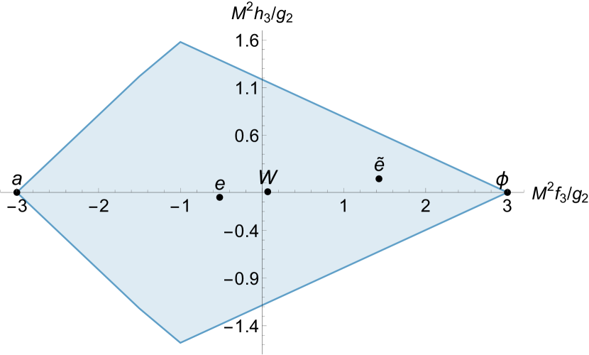
Figure 3: Some bounds on the six-derivative term $M^{2}h_{3}/g_{2}$. The dots refer to the partial UV completions as above.

$$h_{3}= \int_{M^{2}}^{\infty}\frac{dm^{2}}{m^{8}}\bigg{(}\sum_{X}0|c_{0,X}^{0}|^{2}+\sum_{\ell=0,2,\ldots}\sum_{X}0|c^{-}_{\ell,X}|^{2}+\sum_{\ell=3,5,\ldots}\sum_{X}0|c^{o}_{\ell,X}|^{2}$$ (62)

$$+\sum_{\ell=2,4,\ldots}\sum_{X}(\boldsymbol{c}_{\ell,X}^{+})^{\dagger}\frac{1}{2}\left(\begin{array}[]{cc}0&\sqrt{(\ell-1)\ell(\ell+1)(\ell+2)}\\ \sqrt{(\ell-1)\ell(\ell+1)(\ell+2)}&0\\ \end{array}\right)({\boldsymbol{c}_{\ell,X}^{+}})\bigg{)}\,.$$ (65)

In figure 3 we give some examples of bounds derived when including the sum rule (62) in the set of sum rules and null constraints. We include in the plots the values of some known partial UV completions (table 3), which consist of integrating out massive fields at tree- and loop-level. The notations in the plots for them is the following: massive axion ($a$), scalar ($\phi$), graviton ($h$), QED ($e$), scalar QED ($\tilde{e}$) and $W^{\pm}$ sector ($W$).

Another novelty with respect to our previous work is that we are not building crossing-invariant sum rules as before. This leads to a number of new null constraints, so in general the bounds will be stronger than those found in Henriksson:2021ymi . For instance, we can make use of a new null constraint of order $m^{-6}$,

$$0 =\int_{M^{2}}^{\infty}\frac{dm^{2}}{m^{6}}\bigg{(}\sum_{X}0|c_{X,0}^{+}|^{2}+\sum_{\ell=2,4,\ldots}\sum_{X}(\boldsymbol{c}_{\ell,X}^{+})^{\dagger}\left(\begin{array}[]{cc}\ell(\ell+1)&0\\ 0&(\ell^{2}+\ell-7)\\ \end{array}\right)\boldsymbol{c}_{\ell,X}^{+}$$ (68)

$$\quad+\sum_{\ell=0,2,\ldots}\sum_{X}|c^{-}_{\ell,X}|^{2}\ell(\ell+1)+\sum_{\ell=3,5,\ldots}\sum_{X}|c^{o}_{\ell,X}|^{2}(\ell^{2}+\ell-7)\bigg{)}\,,$$ (69)

which immediately gives an improved bound for $g_{3}/g_{2}$. Previously, while the upper bound $g_{3}/g_{2}\leqslant 1/M^{2}$ was found without null constraints, the lower bound $g_{3}/g_{2}\geqslant-4.82/M^{2}$ required the use of null constraints at order $m^{-8}$ and higher, and the precise value of that bound depended on the number of null constraints used. Now, using the non-crossing symmetric sum rules, and therefore the new null constraint at order $m^{-6}$, we are able to obtain both an upper and lower bound which does not improve when adding more null constraints. The new optimal bound is

$$-\frac{1}{M^{2}}\,\leqslant\,\frac{g_{3}}{g_{2}}\,\leqslant\,\frac{1}{M^{2}}\,.$$ (70)

In fact, this is just the first instance of an infinite sequence of two-sided bounds involving the coefficients of the powers of $s^{p}$ in the amplitude $g(s|t,u)$, as shown in (167) in appendix A.

Moving to eight-derivative order, we can see that our new approach significantly reduces the allowed region in the plane given by $g_{4,1}$ and $g_{4,2}$, see figure 4. More precisely, the new allowed region fits into a triangle determined by the inequalities

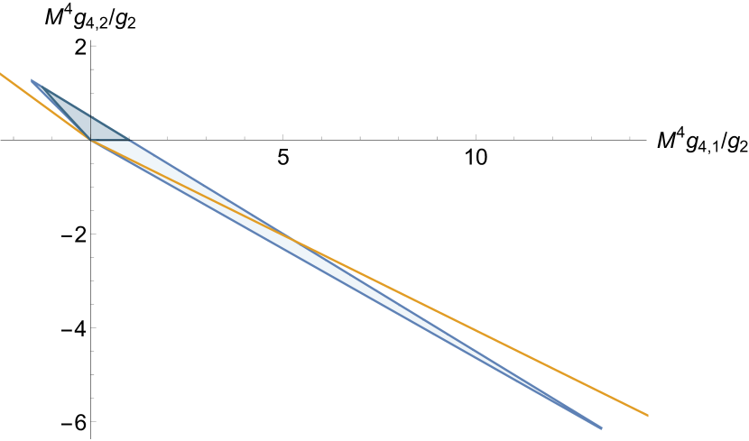
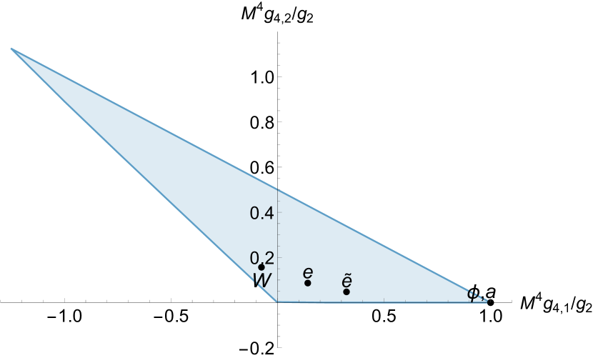
Figure 4: Allowed region in the space $(M^{4}g_{4,1}/g_{2},M^{4}g_{4,2}/g_{2})$. In the left figure we show in orange the one sided bound (allowed above, disallowed below) from Arkani-Hamed:2020blm , in light blue the result from Henriksson:2021ymi and in dark blue our new result. In the other figure we zoom in the new allowed region, adding some partial completions 3.

$$0\,\leqslant\,\frac{2g_{4,2}}{g_{4,1}+2g_{4,2}}\,\leqslant\,\frac{12}{5},\qquad 0\,\leqslant\,\frac{g_{4,1}+2g_{4,2}}{g_{2}}\,\leqslant\,\frac{1}{M^{4}}\,.$$ (71)

The previous available bounds were $-\frac{370}{29}\leqslant\frac{2g_{4,2}}{g_{4,1}+2g_{4,2}}\leqslant\frac{18}{7}$, $0\leqslant\frac{g_{4,1}+2g_{4,2}}{g_{2}}\leqslant\frac{1}{M^{4}}$ from Henriksson:2021ymi (light blue) and $-\frac{30}{7}\leqslant\frac{2g_{4,2}}{g_{4,1}+2g_{4,2}}\leqslant 6$, $g_{4,1}+2g_{4,2}\geqslant 0$ from Arkani-Hamed:2020blm (yellow line).

Additional bounds involving more EFT coefficients are given in Appendix B. The plots are obtained using all the 15 null constraints up to order $m^{-12}$ and setting $\ell_{max}=40$.

3 Results with Gravity

In this section we turn to the main novelty of this paper, which is bounds on the EFT coefficients that describe photon amplitudes in the presence of gravity. These bounds are derived via integral sum rules Caron-Huot:2021rmr ; Caron-Huot:2022ugt , which provide a way to circumvent the problem with the graviton pole. In four dimensions, using such sum rules introduces a logarithmic dependence on an infrared cutoff $m_{\mathrm{IR}}$. The details on how to derive such bounds will be laid out below; here we will summarize the main results.

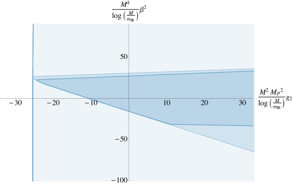
Figure 5: Exclusion plot in the plane $(g_{2},\beta^{2})$ properly normalized and divided by $\log(M/m_{\mathrm{IR}})$. The shaded regions represent the allowed values obtained by using various combinations of dispersion relations. In particular the light blue only uses the $\mathcal{I}_{g}$ dispersion relation, while the darker blue uses the $\mathcal{I}_{g}$,$\mathcal{I}_{0}$ and the $\mathcal{I}_{g}$, $\mathcal{I}_{0}$, $\mathcal{I}_{\beta^{2}}$ dispersion relations. The bounds have been obtained in the parametric limit $\log(M/m_{\mathrm{IR}})\gg 1$.

Our most interesting result is that we find that the positivity approach used in this paper cannot rule out violations to the black hole weak gravity conjecture. Specifically, we find that the coefficient $g_{2}$ must satisfy an inequality of the form

$$g_{2}\geqslant-\frac{c_{1}}{M^{2}M_{\mathrm{P}}^{2}}\log\left(\frac{M}{m_{\mathrm{IR}}}\right)+\frac{c_{0}}{M^{2}M_{\mathrm{P}}^{2}}\,,$$ (72)

where $c_{1}=24.257$ and $c_{0}=33.328$. Moreover, assuming that $\beta=0$, this inequality is strengthened to

$$g_{2}\geqslant-\frac{\tilde{c}_{1}}{M^{2}M_{\mathrm{P}}^{2}}\log\left(\frac{M}{m_{\mathrm{IR}}}\right)+\frac{\tilde{c}_{0}}{M^{2}M_{\mathrm{P}}^{2}}\,,\qquad(\beta=0)\,,$$ (73)

where now $\tilde{c}_{1}=-10.557$ and $\tilde{c}_{0}=11.659$. We can also construct bounds in the plane $g_{2},\,\beta^{2}$ by considering arbitrary values of the ratio $\beta^{2}M_{\mathrm{P}}^{2}/(g_{2}M^{2})$. In figure 5 we present such bounds in the limit $m_{\mathrm{IR}}\to 0$, where the IR logarithm dominates.

The rest of this section will be devoted to a detailed description of how to obtain bounds in the presence of gravity. In section 3.1 we outline the method used to generate the bounds in (72)–(73) and figure 5. Then in section 3.2.1 we present a completely explicit functional that gives a weaker version of the bound (72). The stronger bound (72) is simply found by extending this method to allow for more complicated functionals.

In section 3.4 we make an interpretation of our bounds. It is noteworthy that the violations to the black hole gravity conjecture vanish in the limit $M^{2}/M_{\mathrm{P}}^{2}\to 0$. By assuming a scaling that is compatible with integrating out charged matter, which covers the case of QED, we find that in this limit the usual QED positivity bounds such that $g_{2}\geqslant 0$ are recovered. In the limit where the electromagnetic strength becomes comparable to the gravitational, the bound (73) applies, and negative values of $g_{2}$ cannot be ruled out.

3.1 Method

By using the general formalism laid out in the last subsection of appendix A, integral sum rules can be derived. By taking suitable linear combinations of them (and some of the higher sum rules), we write down the following useful integral sum rules, which we compactly collect into a vector equation

$$\vec{\mathcal{I}}|_{\mathrm{low}}= \int_{M^{2}}^{\infty}\frac{dm^{2}}{m^{2}}\bigg{(}\sum_{X}|c_{0,X}^{0}|^{2}\vec{V}^{0}_{0,m^{2},u}+\sum_{\ell=2,4,\ldots}\sum_{X}\sum_{a,b=1}^{2}(c_{\ell,X}^{+})^{a}({c_{\ell,X}^{+}}^{*})^{b}(\vec{V}^{+}_{\ell,m^{2},u})^{ab}$$

$$+\sum_{\ell=0,2,\ldots}\sum_{X}|c^{-}_{\ell,X}|^{2}{\vec{V}^{-}_{\ell,m^{2},u}}+\sum_{\ell=3,5,\ldots}\sum_{X}|c^{o}_{\ell,X}|^{2}{\vec{V}^{o}_{\ell,m^{2},u}}\,.$$ (74)

In the above equation we have introduced the vector of low-energy coefficients $\vec{\mathcal{I}}|_{\mathrm{low}}$, a vector of $2\times 2$ matrices $\vec{V}^{+}_{\ell,m^{2}}$ and the two vectors $\vec{V}^{-}_{\ell,m^{2},u}$ and $\vec{V}^{o}_{\ell,m^{2},u}$. Notice also that the presence of three positive spectral densities $|c_{0,X}^{0}|^{2},|c_{\ell,X}^{-}|^{2}$ and $|c_{\ell,X}^{o}|^{2}$ and the two-dimensional vector $(c_{\ell,X}^{+})^{a}$. The low-energy part of (74) is a vector given by

$$\vec{\mathcal{I}}|_{\mathrm{low}}=\left\{\mathcal{I}_{g}|_{\mathrm{low}},\,\mathcal{I}_{f}|_{\mathrm{low}},\,\mathcal{I}_{h}|_{\mathrm{low}},\,\mathcal{I}_{0}|_{\mathrm{low}},\,\mathcal{I}_{\beta^{2}}|_{\mathrm{low}}\right\}^{T},$$ (75)

where

$$\begin{split}\mathcal{I}_{g}|_{\mathrm{low}}&=-\frac{1}{M_{\mathrm{P}}^{2}}\frac{1}{u}+g_{2}-4\frac{\beta^{2}}{M_{\mathrm{P}}^{2}}u\,,\\ \mathcal{I}_{f}|_{\mathrm{low}}&=f_{2}-5\frac{\beta^{2}}{M_{\mathrm{P}}^{2}}u-\frac{u}{2}f_{3}\,,\\ \mathcal{I}_{h}|_{\mathrm{low}}&=\frac{\beta}{M_{\mathrm{P}}^{2}}-\frac{u}{2}h_{3}\,,\\ \mathcal{I}_{0}|_{\mathrm{low}}&=0\,,\\ \mathcal{I}_{\beta^{2}}|_{\mathrm{low}}&=\frac{\beta^{2}}{M_{\mathrm{P}}^{2}}u\,.\end{split}$$ (76)

The high-energy part of (74) contains the four vectors

$$\vec{V}^{0}_{0,m^{2},u} =\left\{\frac{1}{m^{4}},\frac{1}{m^{4}}-\frac{3u}{2m^{6}},0,0,0\right\}^{T}\,,$$ (77)

$$\vec{V}^{+}_{\ell,m^{2},u} =\left\{\begin{pmatrix}I_{g,1}&0\\ 0&I_{g,2}\end{pmatrix},\begin{pmatrix}I_{f}&0\\ 0&0\end{pmatrix},\begin{pmatrix}0&I_{h}\\ I_{h}&0\end{pmatrix},\begin{pmatrix}I_{0,1}&0\\ 0&I_{0,2}\end{pmatrix},\begin{pmatrix}I_{\beta^{2},1}&0\\ 0&I_{\beta^{2},2}+I_{\beta^{2},3}\end{pmatrix}\right\}^{T}\,,$$ (78)

$$\vec{V}^{-}_{\ell,m^{2},u} =\left\{I_{g,1}\,,\,-I_{f}\,,\,0\,,\,I_{0,1}\,,\,I_{\beta^{2},1}\right\}^{T}\,,$$ (79)

$$\vec{V}^{o}_{\ell,m^{2},u} =\left\{I_{g,2}\,,\,0\,,\,0\,,\,I_{0,2}\,,\,I_{\beta^{2},2}-I_{\beta^{2},3}\right\}^{T}\,,$$ (80)

where

$$\begin{split}I_{g,1}&=\frac{u+m^{2}{{}_{2}F_{1}}\left(-\ell,\ell+1;1;-\frac{u}{m^{2}}\right)}{m^{4}(u+m^{2})}\,,\\ I_{g,2}&=\frac{u+(u-m^{2}){{}_{2}F_{1}}\left(2-\ell,\ell+3;1;-\frac{u}{m^{2}}\right)}{m^{4}(u-m^{2})}\,,\\ I_{f}&=\frac{\ell(\ell+1)u^{3}}{m^{6}(u^{2}-m^{4})}-\frac{u^{2}(3u+4m^{2})}{2m^{6}(u+m^{2})^{2}}+\frac{m^{4}(u+2m^{2})}{2m^{6}(u+m^{2})^{2}}{{}_{2}F_{1}}\left(-\ell,\ell+1;1;-\frac{u}{m^{2}}\right)\,,\\ I_{h}&=\sqrt{(\ell-1)\ell(\ell+1)(\ell+2)}\frac{2u^{3}+u(u^{2}+m^{2}u-2m^{4}){{}_{2}F_{1}}\left(2-\ell,3+\ell;3;-\frac{u}{m^{2}}\right)}{8m^{6}(m^{4}-u^{2})}\,,\\ I_{0,1}&=\frac{\ell(\ell+1)u^{2}}{m^{6}(u+m^{2})}+\frac{u-u\,{{}_{2}F_{1}}\left(-\ell,\ell+1;1;-\frac{u}{m^{2}}\right)}{m^{2}(u+m^{2})^{2}}\,,\\ I_{0,2}&=\frac{\ell(\ell+1)u^{2}}{m^{6}(u-m^{2})}+\frac{u\left(m^{2}-7u+(u-m^{2}){{}_{2}F_{1}}\left(2-\ell,\ell+3;1;-\frac{u}{m^{2}}\right)\right)}{m^{6}(u-m^{2})}\,,\\ I_{\beta^{2},1}&=\frac{\ell(\ell+1)u^{2}}{4m^{6}(m^{2}-u)}\,,\\ I_{\beta^{2},2}&=\frac{u^{2}(7u+8m^{2})}{4m^{6}(u+m^{2})^{2}}-\frac{\ell(\ell+1)u^{2}}{4m^{6}(u+m^{2})}\,,\\ I_{\beta^{2},3}&=\frac{(\ell-1)\ell(\ell+1)(\ell+2)u^{2}(u+2m^{2})}{96m^{6}(u+m^{2})^{2}}{{}_{2}F_{1}}\left(2-\ell,\ell+3;5;-\frac{u}{m^{2}}\right)\,.\end{split}$$ (81)

Here we used the formula (144) for the Wigner $d$ functions.

3.1.1 Algorithm

In order to obtain bounds on the low-energy parameters (75), we act on the vector dispersion relation (74) with a functional $\Lambda$ and demand positivity of each term appearing on the right-hand side of the equation. If such a functional exists, it will produce a constraint on the low-energy parameters $g_{2}$, $f_{2}$, $\beta$, $g_{3}$, etc., in terms of the parameters $M$, $M_{\mathrm{P}}$ and $m_{\mathrm{IR}}$.

More concretely, we consider functionals of the form

$$\Lambda\left[\vec{f}\right]=\sum_{i}\Lambda_{i}\left[f_{i}\right]\,,\qquad\Lambda_{i}\left[f(p^{2})\right]=\int_{m_{\mathrm{IR}}}^{M}\phi(p)f(p)dp\,,$$ (82)

$$\phi(p)=\sum_{q_{n}\in\mathcal{S}_{i}}c_{n,i}\,q_{n}(p)\,,$$ (83)

where $\mathcal{S}_{i}$ is a set of functions $q_{n}(p)$ in the variable $p$. Each $q_{n}$ contains integer or half-integer powers of $p$. We will discuss the choice of these sets in the next section. The index $i$ runs over any non-empty subset of $\{1,2,3,4,5\}$. For instance, in section 3.2.1 and section 3.2.2 we will consider functionals using respectively only $i=1$ and $i=1,2$.

The lower extreme of integration in (82) deserves special attention. We will discuss it in the next sections. Let us first spell out the concrete algorithm:

1. Choose a subset of dispersion relation to use. This corresponds to selecting which of the $\Lambda_{i}$ appear in (82).

2. Check if there exists a choice of coefficients $c_{n,i}$ such that:

   $$\begin{split}\Lambda[\vec{V}^{+}_{0,m^{2},u}]&\geqslant 0\qquad\text{for all }m^{2}\geqslant M^{2}\,,\\ \Lambda[\vec{V}^{+}_{\ell,m^{2},u}]&\succcurlyeq 0\qquad\text{for all }m^{2}\geqslant M^{2},\ \ell=2,4,\ldots\,,\\ \Lambda[\vec{V}^{-}_{\ell,m^{2},u}]&\geqslant 0\qquad\text{for all }m^{2}\geqslant M^{2},\ \ell=0,2,\ldots\,,\\ \Lambda[\vec{V}^{o}_{\ell,m^{2},u}]&\geqslant 0\qquad\text{for all }m^{2}\geqslant M^{2},\ \ell=3,5,\ldots.\end{split}$$ (84)

3. If such a functional exists then we obtain the constraint

   $$\Lambda[\vec{\mathcal{I}}|_{\mathrm{low}}]=\frac{1}{M^{2}_{\textrm{P}}}\Lambda_{1}[p^{-2}]+g_{2}\Lambda_{1}[1]+\frac{\beta^{2}}{M^{2}_{\textrm{P}}}\Lambda_{1}[4p^{2}]+\ldots+\frac{-\beta^{2}}{M^{2}_{\textrm{P}}}\Lambda_{5}[p^{2}]\geqslant 0\,,$$ (85)

   where the $\ldots$ includes the other low-energy coefficients, if present. There is a constraint for any functional satisfying (84).

4. In order to obtain the optimal constraint on a given parameter, say $g_{2}$, one can fix the values of the other parameters ($\beta=\beta_{*},f_{2}=f_{2*}$, etc) and choose the functional that optimizes the following conditions:

   $$\Lambda_{1}[1]=\pm 1\quad\mathrm{(normalization)}\,,$$ (86)

   $$\mathrm{maximize}\,\,-\Lambda[\vec{\mathcal{I}}|_{\mathrm{low}}]\bigg{|}_{g_{2}=0,\beta=\beta_{*},\ldots}\,.$$ (87)

   Then

   $$g_{2}\gtreqless\mp\Lambda[\vec{\mathcal{I}}|_{\mathrm{low}}]\bigg{|}_{g_{2}=0,\beta=\beta_{*},\ldots}\,.$$ (88)

   In this way one obtains a bound on $g_{2}$ for fixed $\beta_{*},f_{2*},$ etc. By scanning over them one gets bounds as a function of the other parameters. Similarly one can obtain bounds on any other parameter.

3.1.2 Positivity

In order to implement the algorithm, we need to find a method to impose positivity on the whole parameter space in the high-energy regime. Specifically, we need to impose that the functional is positive in all of the following regions, see figure 6,

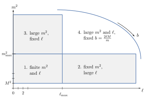
Figure 6: We will demand positivity in the regimes indicated.

1. Finite $\ell$ and $m^{2}$,

2. Large $\ell$ fixed $m^{2}$,

3. Fixed $\ell$, large $m^{2}$,

4. Large $\ell$ and $m^{2}$, for fixed (dimensionless) impact parameter $b=\frac{2\ell M}{m}$.

Demanding positivity in the first three regions in the numerical implementation is a standard task and is achieved by a suitable discretization. We give more details about this in appendix C. The fourth region, namely in the limit of large $\ell$ and $m^{2}$ for fixed impact parameter $b$, requires a very careful consideration, which will be the topic of the remainder of this subsection.

3.1.3 Large-$\ell,m^{2}$ behavior and choice of functionals

As explained in Caron-Huot:2021rmr , the major obstruction in getting a positive functional comes from the tension between the need to cancel the oscillating behavior of the hypergeometric functions at large $\ell$ and the need to have convergent integrals in $p$. Let us review this problem and see how we can choose the functionals $\Lambda_{i}$.

To study more carefully the limit of large $\ell$, we introduce the (dimensionless) impact parameter $b=2\ell M/m$ and consider the behavior of the terms in the dispersion relation in the limit of large $\ell$, large $m$ and fixed $b$. In order to extract the leading behavior, we need the known limit of hypergeometric functions. More precisely we need the asymptotics of the expression

$$C_{\nu,n}(b)=\lim_{m^{2},\ell\to\infty}\int_{0}^{M}dp\,\frac{p^{n}}{M^{n+1}}{{}_{2}F_{1}}\left(a_{1}-\ell,a_{2}+\ell,\nu,\frac{p^{2}}{m^{2}}\right)\,,$$ (89)

where the limit is taken for fixed $b=\frac{2\ell M}{m}$, and we have indicated that this limit is independent of the finite shifts $a_{1}$ and $a_{2}$. We use the following formula, extracted from Thorsley2001

$$J_{\nu-1}(z)=\frac{\left(\frac{z}{2}\right)^{\nu-1}}{\Gamma(\nu)}\lim_{|\lambda|,|\mu|\to\infty}{{}_{2}F_{1}}\left(\lambda,\mu;\nu;-\frac{z^{2}}{4\lambda\mu}\right),$$ (90)

where $J_{n}$ is a Bessel function. Applying it to (89), we find

$$C_{\nu,n}(b)=\frac{\Gamma(\nu)}{(b/2)^{\nu-1}}\int_{0}^{M}dp\,\frac{p^{n+1-\nu}}{M^{n+2-\nu}}J_{\nu-1}(bp/M)\,.$$ (91)

Using the expression for the integral of $p^{a}J_{k}(bp/M)$ (which is a known integral, convergent for $n>-1$ and implemented for instance in Mathematica), we get

$$C_{\nu,n}(b)=\frac{1}{n+1}{{}_{1}F_{2}}\left(\frac{n+1}{2};\frac{n+3}{2},\nu;-\frac{b^{2}}{4}\right)\,.$$ (92)

Given our ansatz (82) for the functional $\Lambda$, we need to consider the large spin limit of the elementary integrals $p^{n}\vec{V}^{+}_{\ell,m^{2},-p^{2}}$, $p^{n}\vec{V}^{-}_{\ell,m^{2},-p^{2}}$ and $p^{n}\vec{V}^{o}_{\ell,m^{2},-p^{2}}$. For the moment let us take the lower extreme of the integral $m_{\mathrm{IR}}=0$. Using the above results we obtain

$$\int_{0}^{1}dp\,p^{n}\!\lim_{j,m\to\infty}\!\vec{V}^{+}_{\ell,m^{2}} ={\small\left\{\!\begin{pmatrix}C_{0,n}&0\\ 0&C_{0,n}\end{pmatrix}\!,\!\begin{pmatrix}C_{0,n}&0\\ 0&0\end{pmatrix}\!,\!\begin{pmatrix}0&0\\ 0&0\end{pmatrix}\!,\!\begin{pmatrix}C_{2,n}&0\\ 0&C_{2,n}\end{pmatrix}\!,\!\begin{pmatrix}0&0\\ 0&C_{4,n}\end{pmatrix}\!\right\}^{\!T}}\!\frac{b^{4}}{16\ell^{4}}+\ldots\,,$$ (93)

$$\int_{0}^{1}dp\,p^{n}\!\lim_{j,m\to\infty}\!\vec{V}^{-}_{\ell,m^{2}} =\left\{C_{0,n},-C_{0,n},0,0,0\right\}^{T}\frac{b^{4}}{16\ell^{4}}+\ldots\,,$$ (94)

$$\int_{0}^{1}dp\,p^{n}\!\lim_{j,m\to\infty}\!\vec{V}^{o}_{\ell,m^{2}} =\left\{C_{0,n},0,0,0,-C_{4,n}\right\}^{T}\frac{b^{4}}{16\ell^{4}}+\ldots\,,$$ (95)

where for simplicity we put $M=1$ and omitted the $b$ dependence inside $C_{\nu,n}$.

Let us begin by focusing on the $\mathcal{I}_{g}$ dispersion relation only, namely the first entry of (74), discarding the others for the moment. In this case the asymptotic behavior is controlled by $C_{0,n}$. The functional $\Lambda\equiv\Lambda_{1}$ should then satisfy (in addition to other conditions)

$$\sum_{n}a_{n}C_{0,n}(b)\geqslant 0\,,\quad\text{for any }b\geqslant 0\,,$$ (96)

where the $a_{n}$ are linearly related the coefficients $c_{n,1}$ appearing in (82) by the actual choice of functions $q_{n}\in\mathcal{S}_{1}$.

Inspecting the large $b$ expansion of $C_{0,n}(b)$, one observes potentially dangerous oscillating terms:

$$C_{0,n}(b)\simeq\frac{1}{b^{n+1}}\frac{2^{n}\Gamma\left(\frac{n+1}{2}\right)}{\Gamma\left(\frac{1-n}{2}\right)}+\frac{\sin(b)-\cos(b)}{\sqrt{\pi}b^{3/2}}+\frac{(8n-5)(\sin(b)+\cos(b))}{8\sqrt{\pi}b^{5/2}}+O(b^{-7/2})\,,$$ (97)

where the higher order terms correspond to half-integer powers only. In order to have a chance to fulfill the positivity condition one must suppress the oscillating behavior. One possibility would be to include, in the set $\mathcal{S}_{1}$, a power $n<1/2$ such that the first non-oscillating term in (97) could dominate over the rest. Unfortunately in four dimensions the integral of such a term would produce a divergence in the low-energy part of the dispersion relation due to the graviton pole:

$$\int_{0}^{M}\frac{p^{n}}{p^{2}}\frac{dp}{M_{\mathrm{P}}^{2}}<\infty\ \iff\ n>1\,.$$ (98)

Alternatively, following Caron-Huot:2021rmr , we can engineer a linear combination to cancel the leading oscillating terms. For numerical reasons it is convenient (although not necessary) not to introduce integer powers but to preserve the expansion in half-integer powers only. Hence the smallest power at our disposal is $n=3/2$. In order to have this term dominate at large $b$ we must cancel the first two oscillating terms. We also note that when $n$ is an odd positive integer, the first term in (97) vanishes, thus we can use two such powers and create the combinations

$$C_{0,n}(b)+\frac{1}{2}(n-5)C_{0,3}(b)-\frac{1}{2}(n-3)C_{0,5}(b)\simeq\frac{1}{16b^{n+1}}\frac{2^{n}\Gamma\left(\frac{n+1}{2}\right)}{\Gamma\left(\frac{1}{2}-\frac{n}{2}\right)}+O(b^{-7/2})\,.$$ (99)

This corresponds to considering functionals with polynomials

$$q_{n}(p)=(p/M)^{n}+\frac{1}{2}(n-5)(p/M)^{3}-\frac{1}{2}(n-3)(p/M)^{5}\,.$$ (100)

One can show that the oscillating behavior at large $b$ in (96) is produced by the upper extreme of integration: the faster $q_{n}(p)$ goes to zero as $p\to M$, the more suppressed are the oscillations. Our choice of functionals satisfies $q_{n}(p)=O(M-p)^{2}$.

Note that at this point the condition (96) is asymptotically achieved by taking the coefficient multiplying $q_{3/2}$ negative, since $\Gamma(-1/4)<0$ in (99).

3.1.4 Reintroducing the IR cut-off

Unfortunately, the above discussion does not hold for finite values of the dimensionless impact parameter $b$. As discussed in Caron-Huot:2021rmr , there exists a tension between the conditions (96) and (98) – the two conditions are mutually exclusive. This fact is made manifest when passing to the impact parameter space by taking the two dimensional Fourier transform of a function of the transverse momentum $\vec{p}$:

$$\widetilde{\phi}(b)=\int d^{2}p\frac{\phi(p)}{2\pi p}e^{i\vec{b}\cdot\vec{p}/M}=\Gamma\left(\frac{1}{2}\right)\int_{0}^{\infty}dp\,\phi(p)J_{0}(pb/M)\,,$$ (101)

where again $J_{0}$ is the Bessel function which also appears in the large $\ell$ limit (89). Recalling the definition of our functional $\Lambda$, we can interpret the positivity conditions in the large $m,\ell$ limit as the condition

$$\widetilde{\phi}(b)>0\quad\text{for any }b\geqslant 0\,.$$ (102)

On the other hand, the finiteness of the functional on the gravity pole (98) would require

$$0=\lim_{p\to 0}\frac{\phi(p)}{p}\propto\int_{0}^{\infty}d^{2}b\widetilde{\phi}(b)\,.$$ (103)

Clearly the conditions (102) and (103) are incompatible. As a consequence, in order to proceed further we must relax one of the two conditions. Given the presence of IR divergences in gravity, it seems natural to introduce an IR regulator in the form of a maximal impact parameter $b_{\text{max}}$ that can be probed by the scattering process. If that were the case, we would only need to demand positivity of $C_{0,n}(b)$ for $b\leqslant b_{\text{max}}$. In principle we could search for functionals subject to this reduced positivity condition and obtain bounds as a function of $b_{\text{max}}$.

However, is more convenient to introduce an IR cutoff as a regulator $m_{\mathrm{IR}}>0$ at small momenta as in (82). This modification gets rid of the restriction (98) on the polynomials $q_{n}$, since now all the integrals are finite, but at the same time makes the bounds on couplings explicitly dependent on $m_{\mathrm{IR}}$. More precisely, including a term $q_{n}$ with $n<1$ introduces factors of the form $(M/m_{\mathrm{IR}})^{1-n}$. A milder dependence on the cut-off can be obtained by only including $q_{1}$, which instead gives a logarithmic dependence in (85)

$$\Lambda[\vec{\mathcal{I}}|_{\mathrm{low}}]\supset c_{1,1}\int_{m_{\mathrm{IR}}}^{M}\frac{q_{1}(p)}{p^{2}M_{\mathrm{P}}^{2}}\frac{dp}{M}\simeq\frac{c_{1,1}}{M^{2}M_{\mathrm{P}}^{2}}\left(\log\left(\frac{M}{m_{\mathrm{IR}}}\right)-\frac{1}{4}+O\left(\frac{m_{\mathrm{IR}}}{M}\right)\right)\,.$$ (104)

In conclusion, our tentative choice for the polynomials in $\mathcal{S}_{1}$ is

$$\mathcal{S}_{1}=\big{\{}\left(\frac{p}{M}\right)^{n}+\frac{1}{2}(n-5)\left(\frac{p}{M}\right)^{3}-\frac{1}{2}(n-3)\left(\frac{p}{M}\right)^{5};\text{ with }n=1,\frac{3}{2},\frac{5}{2},\frac{7}{2},\ldots\big{\}}\,.$$ (105)

A second important effect of $m_{\mathrm{IR}}$ is that the cancelation of the oscillating terms in (99) is not exact anymore: from the power $p^{n}\subset q_{1}(p)$ one gets a correction to (92) of the form ($\nu=n=1$)

$$\frac{m_{\mathrm{IR}}}{bM}J_{1}\left(b\frac{m_{\mathrm{IR}}}{M}\right)\simeq\frac{1}{2}\left(\frac{m_{\mathrm{IR}}}{M}\right)^{2}+O\left(\frac{bm_{\mathrm{IR}}}{M}\right)\,.$$ (106)

In the large $b$ limit the leading decay is controlled by $b^{-5/2}$, coming from (99) with $n=3/2$, which is comparable to the above correction for

$$b\gtrsim b_{\text{max}}=\left(\frac{M}{m_{IR}}\right)^{4/5}\,.$$ (107)

Hence, the price of regularizing the action of the functional on the graviton pole with an IR cutoff is to introduce a small negativity at large impact parameter. The smaller the cutoff, the farther away we push the negativity, but at the same time we make the bound on the low-energy coefficients less stringent, specifically the bounds will depend logarithmically on $m_{\mathrm{IR}}$.

Finally, let us consider the other dispersion relations in (74): we see that their asymptotic behavior enters with both signs or in the out-of-diagonal components of a matrix. In order for them not to spoil the suppression of large-$b$ oscillations, we must not introduce new dominant contributions. To achieve this, it is enough to cancel the leading universal $b^{-3/2}$ power. Hence we choose:

$$\mathcal{S}_{2}=\mathcal{S}_{4}=\{\left(\frac{p}{M}\right)^{n}-\left(\frac{p}{M}\right)^{3};\text{ with }n=1,\frac{3}{2},\frac{5}{2},\frac{7}{2},\ldots,n_{\text{max}}\}\,,$$ (108)

$$\mathcal{S}_{3}=\{\left(\frac{p}{M}\right)^{n}-\left(\frac{p}{M}\right)^{3};\text{ with }n=\frac{3}{2},\frac{5}{2},\frac{7}{2},\ldots,n_{\text{max}}\}\,,$$ (109)

$$\mathcal{S}_{5}=\{\left(\frac{p}{M}\right)^{n}-\left(\frac{p}{M}\right)^{5};\text{ with }n=\frac{3}{2},\frac{5}{2},\frac{7}{2},\ldots,n_{\text{max}}\}\,.$$ (110)

More details about our numerical setup can be found in Appendix C.

Putting all the pieces together, our approach will then be the following. We will numerically look for a functional of the form (82) (with $m_{\mathrm{IR}}=0$) with the choice of functions $q_{n}$ as in (105) and (108) subject to the conditions (84). This is done by running the numerical semi-definite program solver SDPB Simmons-Duffin:2015qma ; Landry:2019qug . The output of the algorithm are the coefficients $c_{n,i}$ of (82). Taken at face value, such a functional would give a divergent result when applied to $\vec{\mathcal{I}}|_{\text{low}}$. We then modify the functional by taking $m_{\mathrm{IR}}>0$:

$$\Lambda|_{m_{\mathrm{IR}}=0}\longrightarrow\Lambda^{\prime}=\Lambda|_{m_{\mathrm{IR}}>0}\,.$$ (111)

The new functional satisfies $\Lambda^{\prime}[\vec{\mathcal{I}}|_{\text{low}}]=\text{finite}$, and produces bounds with a logarithmic dependence on $m_{\mathrm{IR}}$. On the other hand, the positivity condition is violated at large impact parameter $b\gtrsim b_{\text{max}}$. This is acceptable since it does not make sense to probe infinitely large distances in a theory with an IR cut-off.

3.2 Example bounds from simple functionals

In this section, we will derive two bounds on the four-derivative coefficients by considering two explicit functionals. This will give concrete examples of the considerations above, and produce bounds that share the qualitative features with those presented in figure 5.

3.2.1 Example 1: Global minimum of $g_{2}$

As a first example, we will derive a bound involving $g_{2}$ only, by finding a functional $\Lambda=\Lambda_{1}$ that is manifestly positive. For the sake of simplicity, we take a slightly different form of the functional and allow integer powers. Here we shall only use the sum rules derived from $\mathcal{I}_{g}$. Let us start by the following ansatz:

$$\Lambda_{1}[f]=\int_{m_{\mathrm{IR}}}^{M}\phi(p)f(p)dp\,,\qquad\phi(p)=(M-p)^{3}\sum_{n=1}^{3}c_{n}\left(\frac{p}{M}\right)^{n}\,.$$ (112)

We can fix two of the coefficients to assume that

$$\lim_{m_{\mathrm{IR}}\to 0}\Lambda_{1}[\mathcal{I}_{g}|_{\mathrm{low},g_{2}}]=M^{4},\qquad\lim_{m_{\mathrm{IR}}\to 0}\Lambda_{1}[\mathcal{I}_{g}|_{\mathrm{low},\beta^{2}}]=0\,.$$ (113)

The first condition is just a normalization condition, while the second condition is chosen to produce a bound that is independent of $\beta^{2}$. Solving for $c_{2}$ and $c_{3}$ gives

$$\phi(p)=(M-p)^{3}\frac{p}{M}\left(c_{1}+\frac{p}{M}\frac{2100-51c_{1}}{8}+\frac{p^{2}}{M^{2}}\frac{63(c_{1}-60)}{8}\right)\,.$$ (114)

At this point we first look for a functional that satisfies all the positivity conditions (84) in the limit $m_{\mathrm{IR}}\to 0$; this is done in the next sub-section. Once we have found it, we can now use the same value of $c_{1}$ to define a functional $\Lambda^{\prime}_{1}$ where now $m_{\mathrm{IR}}$ is kept small but finite. As explained in the previous section, the newly defined functional mildly violates the positivity conditions (84) at large $m^{2}$, $\large\ell$ and large impact parameter. Neglecting this violation, we get $\Lambda^{\prime}_{1}[\mathcal{I}_{g}|_{\mathrm{low}}]\gtrsim 0$, with

$$\Lambda^{\prime}_{1}[\mathcal{I}_{g}|_{\mathrm{low}}]=M^{4}g_{2}+\frac{M^{2}}{M_{\mathrm{P}}^{2}}\left(42-\frac{91}{30}c_{1}+c_{1}\log\left(\frac{M}{m_{\mathrm{IR}}}\right)\right)+O(m_{\mathrm{IR}}/M)\,,$$ (115)

and in the parametric limit $m_{\mathrm{IR}}/M\to 0$ where the log dominates, we would get the bound

$$\Lambda_{1}[\mathcal{I}_{g}|_{\mathrm{low}}]\geqslant 0\quad\Rightarrow\quad g_{2}\geqslant-\frac{c_{1}}{M^{2}M_{\mathrm{P}}^{2}}\log\left(\frac{M}{m_{\mathrm{IR}}}\right)\,.$$ (116)

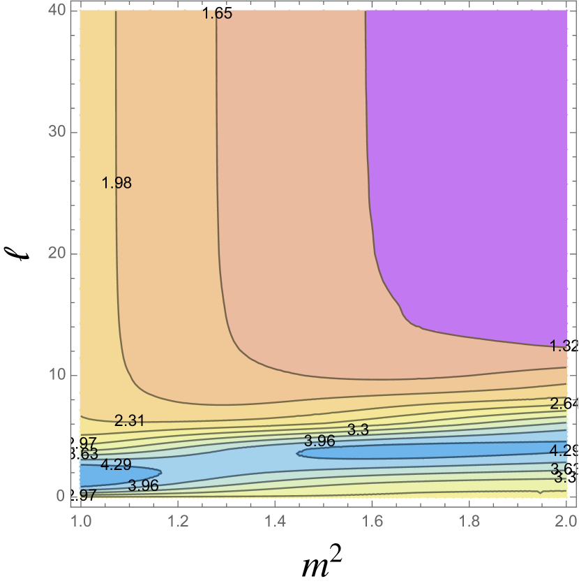
Figure 7: Action of the functional (114) (with $c_{1}=28.0033$) on $I_{g,1}$, see (77) and (81), for finite values of $\ell$ and $m^{2}$. The contours are obtained by interpolating integer values of $\ell$. Similar plots can be obtained for $I_{g,2}$.

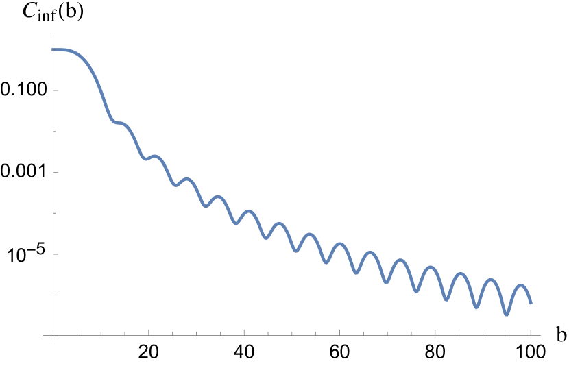
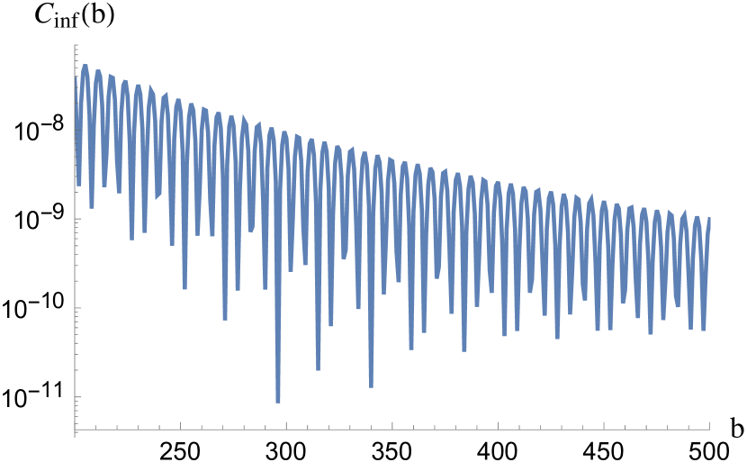
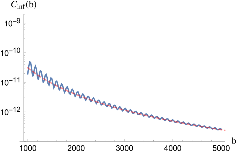
Figure 8: Action of the functional in the limit of large $m^{2}$, large $\ell$, as a function of $b$. Here $\delta=0.0033$. The oscillatory terms become important for $b\sim 10^{2}$ and then gets suppressed compared to the leading $b^{-3}$ behavior (dashed red line), as predicted by (120).

Optimizing over $c_{1}$

We will now look for a functional of the form (114) that is positive on the high-energy part when $m_{\mathrm{IR}}=0$. The strongest bound is derived from the lowest positive value of $c_{1}$, which we denote $c_{1}^{*}$. It turns out that it is the last condition in figure 6, at large $m^{2}$ and $\ell$, that puts the strongest constraints on what $c_{1}$ can be used to find a positive functional. We will examine this limit to find

$$c_{1}^{*}=28+\delta\,,$$ (117)

for a small $\delta$, which has to be numerically determined.

In the high-energy expression (75), there are two different expressions that appear: $I_{g,1}$ and $I_{g,2}$ (81). In the limit of large $\ell$ and $m^{2}$, for fixed impact parameter, these two expressions have the same asymptotic behavior (93)

$$\int_{0}^{M}dp\,\phi(p)I_{g,i}=\frac{b^{4}}{16\ell^{4}}C_{\mathrm{inf}}(b)+O(\ell^{-5}),\qquad i=1,2\,,$$ (118)

with

$$C_{\mathrm{inf}}(b)= c_{1}C_{0,1}(b)-\frac{75}{8}\left(c_{1}-28\right)C_{0,2}(b)+30\left(c_{1}-42\right)C_{0,3}(b)+\left(2205-\frac{175c_{1}}{4}\right)C_{0,4}(b)$$

$$+30\left(c_{1}-56\right)C_{0,5}(b)-\frac{63}{8}\left(c_{1}-60\right)C_{0,6}(b)\,,$$ (119)

and $C_{0,n}$ defined in (89). Given the expansion

$$C_{\mathrm{inf}}(0,b)=\frac{75(c_{1}-28)}{8}\frac{1}{(bM)^{3}}+O(b^{-9/2}),\qquad b\to\infty\,,$$ (120)

we see that for $c_{1}>28$, it is positive in the large $b$ limit. To find a functional that is positive also for finite $b$, we choose $c_{1}^{*}=28+\delta$, and find that $\delta$ can be taken as small as $\delta=0.0033$. Thus we get

$$g_{2}\geqslant-\frac{28+\delta}{M^{2}M_{\mathrm{P}}^{2}}\log\left(\frac{M}{m_{\mathrm{IR}}}\right)\,.$$ (121)

By inspection, we can verify that the action of the functional is positive in the first entry $\vec{V}^{+}_{0,m^{2}},\vec{V}^{+}_{\ell,m^{2}},\vec{V}^{-}_{\ell,m^{2}},\vec{V}^{o}_{\ell,m^{2}}$ and also $C_{\mathrm{inf}}(b)\geqslant 0$ for any value of $b\geqslant 0$. This is shown in figures 7 and 8.

3.2.2 Example 2: Bounds with fixed relation between $g_{2}$ and $\beta^{2}$

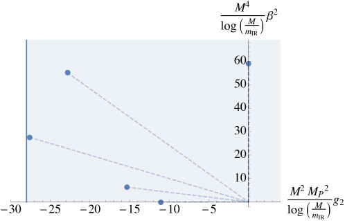
Figure 9: Bounds in the plane $g_{2}M^{2}M^{2}_{\mathrm{P}}/\log(M/m_{\mathrm{IR}})$ vs $\beta^{2}M^{4}/\log(M/m_{\mathrm{IR}})$ in the limit $\log(M/m_{\mathrm{IR}})\gg 1$. The shaded region corresponds to the bound obtained in (121) with $\delta=0.0033$. The circles and the corresponding dashed lines display upper bounds on $\alpha$ in (123).

Now we will instead look at a functional of the form

$$\int_{m_{\mathrm{IR}}}^{M}dp(M-p)^{3}\left(\left(c_{1}\tfrac{p}{M}+c_{2}\tfrac{p^{2}}{M^{2}}+c_{3}\tfrac{p^{3}}{M^{3}}\right)\mathcal{I}_{g}+\left(d_{1}\tfrac{p}{M}+d_{2}\tfrac{p^{2}}{M^{2}}+d_{3}\tfrac{p^{3}}{M^{2}}\right)\mathcal{I}_{0}\right)\,.$$ (122)

We will consider bounds along rays with fixed ratio between $\beta^{2}$ and $g_{2}$. Specifically, we will define

$$g_{2}=\frac{\alpha}{M^{4}}\cos\theta,\qquad\beta^{2}=\frac{\alpha M_{\mathrm{P}}^{2}}{M^{6}}\sin\theta\,,$$ (123)

and maximize the parameter $\alpha$ for a given $\theta$. We can normalize the functional so that the low-energy part gives

$$-\alpha+c_{1}\frac{M^{2}}{M_{\mathrm{P}}^{2}}\log(M/m_{\mathrm{IR}})+\frac{M^{2}}{M_{\mathrm{P}}^{2}}c_{0}+O(m_{\mathrm{IR}}/M)\,,$$ (124)

where $c_{0}$ is a constant. This sets

$$c_{3}=-\frac{3\left(3c_{1}(4\sin\theta+7\cos\theta)+c_{2}(6\sin\theta+7\cos\theta)+420\right)}{10\sin\theta+9\cos\theta}\,,$$ (125)

and for the constant we find

$$c_{0}=-\frac{c_{1}(1179\cos\theta+1208\sin\theta)-24c_{2}(3\cos\theta+4\sin\theta)+3780}{60(9\cos\theta+10\sin\theta)}\,.$$ (126)

The optimal upper bound on $\alpha$ is obtained for the smallest value of $c_{1}$. The algorithm will then be to minimize $c_{1}>0$ while varying $c_{1},c_{2}$, $d_{1}$, $d_{2}$ and $d_{3}$. The results are given in table 2. One can see that they satisfy (125).

Table 2: Functionals of the form (122), and the corresponding bounds. $c_{0}$ is given by (126).

$\theta$	Functional (bound: $\alpha\leqslant\frac{M^{2}}{M_{\mathrm{P}}^{2}}\left(c_{1}\log(M/m_{\mathrm{IR}})+c_{0}\right)$)
$\frac{\pi}{2}$	$c_{1}=58.8508$	$c_{2}=-95.2201$	$c_{3}=-166.4664$	$d_{1}=-855.8213$	$d_{2}=3129.6066$	$d_{3}=-2676.5321$
$\frac{5}{8}\pi$	$c_{1}=59.5901$	$c_{2}=-96.4164$	$c_{3}=-168.5580$	$d_{1}=-866.5732$	$d_{2}=3168.9249$	$d_{3}=-2710.1583$
$\frac{3}{4}\pi$	$c_{1}=39.0239$	$c_{2}=117.0110$	$c_{3}=-377.2315$	$d_{1}=-175.9453$	$d_{2}=643.4036$	$d_{3}=-550.2567$
$\frac{7}{8}\pi$	$c_{1}=16.5636$	$c_{2}=49.6517$	$c_{3}=-21.65410$	$d_{1}=300.0060$	$d_{2}=-760.9365$	$d_{3}=409.8483$
$\pi$	$c_{1}=11.0348$	$c_{2}=33.0782$	$c_{3}=-14.4261$	$d_{1}=199.92585$	$d_{2}=-507.1523$	$d_{3}=273.2191$

With the results found so far we get, in the limit $\log(M/m_{\mathrm{IR}})\to\infty$, the results (121) and the results in table 2. The combined effect of these found are shown in figure 9.

3.3 More results

In this section we present our best bounds on some of the couplings appearing in the low-energy part of the dispersion relations (75). We already showed in figure 5 the constraint on the parameters $g_{2}$ and $\beta^{2}$ obtained acting with a functional on the dispersion relations $\mathcal{I}_{g},\mathcal{I}_{0}$ and $\mathcal{I}_{\beta^{2}}$.

Next, we include in our analysis the dispersion relation $\mathcal{I}_{f}$, which allows us to consider the coefficient $f_{2}$, also appearing in the black hole WGC. More precisely, the black hole WGC would require $g_{2}\pm f_{2}\geqslant 0$, but, as shown in figure 10, the presence of gravity in our setup allows again a violation of the inequality of order $(M/M_{\textrm{P}})^{2}\log(M/m_{\textrm{IR}})$.

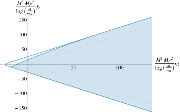
Figure 10: Exclusion plot in the plane $(g_{2},f_{2})$ normalized to $M^{2}M^{2}_{\mathrm{P}}\log(M/m_{\textrm{IR}})$. The shaded regions correspond to assuming $f_{3}\leq 0$ (light blue) or $f_{3}\geq 0$ (dark blue). The former contains the latter. The dashed gray lines indicate the bound without gravity $g_{2}=\pm f_{2}$. This plot used the dispersion relations $\mathcal{I}_{g}$, $\mathcal{I}_{f}$, $\mathcal{I}_{0}$, $\mathcal{I}_{\beta^{2}}$. The minimal value of $g_{2}$ is the same as in Fig. 5 and forces $f_{2}=0,f_{3}\leqslant 0$.

In section 2.3.1 we introduced a method to get bounds on the coefficients $h_{2}=\beta/M_{\mathrm{P}}^{2}$ and $h_{3}$ appearing in the inelastic scattering amplitude such as $\mathcal{M}^{+++-}$, however until now we have not fully exploited this technology, except in absence of gravity in section 2.5. This because the dispersion relations considered so far only depend on positive spectral densities $|c_{\ell,X}^{-}|^{2}$, $|c_{\ell,X}^{+,1}|^{2}$, $|c_{\ell,X}^{+,2}|^{2}$, and $|c_{\ell,X}^{o}|^{2}$.

Thus, as a final application we include the dispersion relation $\mathcal{I}_{h}$ (and drop $\mathcal{I}_{f}$) and consider again bounds on $g_{2}$ and $\beta$. Moreover, we fix $m_{\textrm{IR}}$ to a finite value and inspect the dependence of the bounds on such value. The results are shown in figure 11, for $m_{\textrm{IR}}=10^{-6}M$, $10^{-10}M$. The inclusion of $\mathcal{I}_{h}$ does not substantially improve the bounds, while the finite value of $m_{\textrm{IR}}$ corresponds to a finite shift (which is less and less important since we are plotting the bounds divided by $\log(M/m_{\textrm{IR}}$).

The fact that the bound on $\beta$ does not change in an appreciable way when including the new dispersion relation $\mathcal{I}_{h}$ is a bit surprising. This however is a consequence of the fundamental input from the low-energy EFT which allowed us to relate $\beta\in\mathcal{I}_{h}$ and $\beta^{2}\in\mathcal{I}_{g}$. If we insisted on being agnostic about the interpretation of the low-energy couplings, the inclusion of $\mathcal{I}_{h}$ would still let us bound them separately.

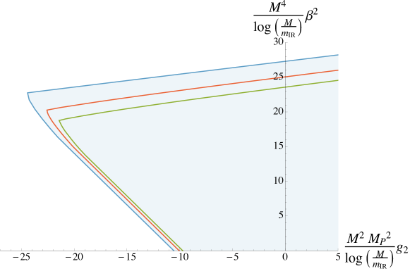
Figure 11: Exclusion plot in the plane $(g_{2},\beta^{2})$ normalised appropriately and divided by $\log(M/m_{\textrm{IR}})$. The shaded region reproduces the best bound from figure 5 while the green and red lines are obtained with finite values of $m_{\textrm{IR}}/M=10^{-6},\,10^{-10}$ and using the dispersion relations $\mathcal{I}_{g}$, $\mathcal{I}_{h}$, $\mathcal{I}_{0}$, $\mathcal{I}_{\beta^{2}}$. Decreasing the value of $m_{\textrm{IR}}$ the bounds shifts towards the blue bound, obtained in the limit $\log(M/m_{\textrm{IR}})\gg 1$. The green and red lines do not change when assuming $h_{3}\geqslant 0$ or $h_{3}\leqslant 0$.

3.4 Violations to the weak gravity conjecture

The purpose of this section has been to derive bounds on the four-derivative corrections to Einstein–Maxwell theory. The most interesting bound, in our opinion, is the lower bound on $g_{2}$, which we find is given by

$$g_{2}\geqslant-24.257\frac{1}{M^{2}M_{\mathrm{P}}^{2}}\log\frac{M}{m_{\mathrm{IR}}}\,.$$ (127)

This bound is determined with the optimization procedure described above and in the appendix, so our conclusion is the following:

The assumptions of this paper, including unitarity, causality, and weak coupling, are not enough to prove the black hole WGC.

In our opinion, this conclusion is not surprising. As we stated in the introduction, it was already anticipated by deRham:2019ctd ; deRham:2020zyh that gravity might weaken causality bounds by introducing time delays. Furthermore, it is consistent with the gravitational weakening of the dispersion-relation bounds for scalars in $d\geqslant 5$ reported in Caron-Huot:2021rmr .

Using this bound requires that we make sense of the logarithmic divergence. Strictly speaking, if we demand that the cutoff may be taken to 0, this bound simply tells us that no constraint may be placed on $g_{2}$. However, we believe that it is possible to do better than this – for instance, it was pointed out in Caron-Huot:2022ugt that even with the conservative estimates $M\sim 1$ TeV and $m_{\mathrm{IR}}$ near the Hubble scale, the resulting $\log 10^{77}$ is not very large. Still, it would be nice to understand what the sharpest possible bounds are, but this will require further assumptions. We comment more on this direction in the conclusion.

Another important assumption is weak coupling, which ensures that EFT loops are suppressed in the amplitudes. This is a rather typical assumption and simply means that we are bounding classical, or tree-level amplitudes. However, in the presence of gravity, it becomes more subtle, because the coupling at low-energy might include factors of the high-energy coupling, or the mass of the high-energy particle. To make this more concrete, consider the EFT which arises from integrating out a charged particle such as an electron or charged scalar. The high-energy loop diagrams which contribute to this may include EM and gravitational couplings, and give rise to four-derivative coefficients which take the form

$$g_{2} =\hat{g}_{2}\frac{\alpha^{2}}{M^{4}}+\hat{g}_{2}^{\prime}\frac{\alpha}{M^{2}M_{\mathrm{P}}^{2}}+O\left(\frac{1}{M_{\mathrm{P}}^{4}}\right)\,,$$ (128)

$$f_{2} =\hat{f}_{2}\frac{\alpha^{2}}{M^{4}}+\hat{f}_{2}^{\prime}\frac{\alpha}{M^{2}M_{\mathrm{P}}^{2}}+O\left(\frac{1}{M_{\mathrm{P}}^{4}}\right)\,,$$ (129)

$$h_{2} =\frac{\beta}{M_{\mathrm{P}}^{2}}=\hat{\beta}\frac{\alpha}{M^{2}M_{\mathrm{P}}^{2}}+O\left(\frac{1}{M_{\mathrm{P}}^{4}}\right)\,,$$ (130)

where the hatted variables are completely numerical constants, and the $O(1/M_{\mathrm{P}}^{4})$ terms correspond to pure gravitational loops. Here $\alpha$ represents the strength of the electromagnetic coupling, for QED $\alpha=\frac{e^{2}}{4\pi}$. For the cases of a spin-$\frac{1}{2}$ or scalar particle, the values are referred to as QED or scalar QED (sQED), and for these cases the constants take known values Drummond:1979pp ; Cheung:2014ega ,

$$\text{QED}: \hat{g}_{2} =\frac{176}{45} \hat{g}_{2}^{\prime} =-\frac{22}{45\pi} \hat{f}_{2} =-\frac{16}{15} \hat{f}_{2}^{\prime} =0 \hat{\beta} =-\frac{1}{180\pi}\,,$$ (131)

$$\text{sQED}: \hat{g}_{2} =\frac{32}{45} \hat{g}_{2}^{\prime} =-\frac{4}{45\pi} \hat{f}_{2} =\frac{8}{15} \hat{f}_{2}^{\prime} =0 \hat{\beta} =\frac{1}{360\pi}\,.$$ (132)

Our assumptions require that the entire amplitude is weakly coupled, meaning that $\alpha\ll 1$, but the meaning of the bounds (72)–(73) depends on the relative size of $\alpha$ and $\mu=\frac{M^{2}}{M_{\mathrm{P}}^{2}}$. In this language, the bounds are

$$\frac{\mu}{M^{4}}\left(\frac{\alpha^{2}}{\mu}\hat{g}_{2}+\alpha\hat{g}_{2}^{\prime}\right)\geqslant\frac{\mu}{M^{4}}\left(c_{1}\log(M/m_{\mathrm{IR}})+c_{0}\right)\,,$$ (133)

so let us comment on their meaning in the following regimes:

Regime $\boldsymbol{\mu\ll\alpha^{2}}$.

In this case, the $\hat{g}_{2}$ term is larger than everything else in (133), so the bound reduces to the familiar

$$\hat{g}_{2}\geqslant 0\,.$$ (134)

This is equivalent to the regime where gravity decouples, so we recover those bounds from section 2.5. If we integrate out a particle that is light relative to the coupling, i.e.

$$M^{2}\ll\alpha^{2}M_{\mathrm{P}}^{2}\,,\,,$$ (135)

then our results mean that the WGC bounds will be satisfied. This is not so surprising, as such particles already (easily) satisfy the particle form of the WGC.

Regime $\boldsymbol{\mu\sim\alpha^{2}}$.

Let us set $\alpha^{2}=\mu$ and absorb any additional factor in the numerical constants. Then the bound (133) that determines the minimum of $g_{2}$ takes the form

$$\hat{g}_{2}+\alpha\hat{g}_{2}^{\prime}>-c_{1}\log(M/m_{\mathrm{IR}})+c_{0}\,.$$ (136)

In this case, the $\hat{g}_{2}^{\prime}$ term is suppressed relative to the others, so our bound only effectively constrains $\hat{g}_{2}$. As a result, we find

• For any fixed $M/m_{\mathrm{IR}}$, we cannot rule out the possibility that $\hat{g}_{2}$ be negative by an amount given by the right-hand side of (136).

• If $\hat{g}_{2}$ has a component that runs logarithmically with $\log(M/m_{\mathrm{IR}})$, we cannot rule out the possibility that this term can be negative, but it must be $>-c_{1}$.

Regime $\boldsymbol{\mu\gg\alpha^{2}}$.

We are unable to probe this regime, which includes $\mu\sim\alpha$, simply because the left-hand side of  (136) becomes suppressed compared to the right-hand side. Therefore the bounds are trivially satisfied.

3.4.1 Constraints on $\beta^{2}$ and a species bound

Let us also comment on the meaning of our bounds on $\beta^{2}$ in terms of $g_{2}$. The allowed region in the space of these two parameters, visible in figure 5, is quite irregular, but at larger values of $g_{2}$, the slope appears to approach about $0.17$. However, in what follows we will ignore all numbers to focus on the scaling. We find

$$\frac{M^{4}}{\log\frac{M}{m_{\mathrm{IR}}}}\beta^{2}\lesssim\frac{M^{2}M_{\mathrm{P}}^{2}}{\log\frac{M}{m_{\mathrm{IR}}}}g_{2}\,.$$ (137)

In the spirit of the discussion above, let us assume for the moment that these coefficients are dominated by integrating out charged particles at 1-loop level. Then, again ignoring order one numbers, we have

$$\beta\simeq\sum_{\mathrm{species}\ i}\frac{q^{2}_{i}}{m_{i}^{2}}\,,\qquad\qquad g_{2}\simeq\sum_{\mathrm{species}\ i}\frac{q^{4}_{i}}{m_{i}^{4}}+\frac{1}{M_{\mathrm{P}}^{2}}\sum_{\mathrm{species}\ i}\frac{q^{2}_{i}}{m_{i}^{2}}\,.$$ (138)

In this case, $\beta$ comes from triangle-type diagrams with two photons and one graviton attached to the charged loop, and $g_{2}$ gets contributions from those diagrams as well as from simple boxes with all four photons attached to the charged loop.

Let us make the simplifying assumption that there are $n$ different species of charged scalars and they all have an equal value of $z=\sqrt{2}qM_{\mathrm{P}}/m$. Then our schematic bound (137) becomes

$$n^{2}z^{4}\lesssim\frac{M_{\mathrm{P}}^{2}}{M^{2}}(z^{4}+z^{2})n\,.$$ (139)

Here it is possible that $z\gg 1$ (incidentally, this means that the species satisfy the particle WGC, though that is not relevant), in which case the bound on $\beta^{2}$ leads to a simple bound on the number of charged species, $n\lesssim M_{\mathrm{P}}^{2}/M^{2}$. If $z\lesssim 1$, then a bound on the number of charged species still follows, but the actual value of $z$ begins to matter as well.

It is interesting that this bound is highly analogous to the “species bound” Dvali:2007hz ; Dvali:2007wp , which roughly states that the cutoff scale in a EFT with gravity and a large number of species, is given by

$$M\simeq M_{\mathrm{P}}/\sqrt{n}\,.$$ (140)

Our bound may be interpreted as an analogous bound for charged particles. Adding an extra species with $z>1$ contributes more to the $\beta^{2}$ term than to the $g_{2}$ term, so an upper bound on $\beta^{2}$ in terms of $g_{2}$ gives a limit on the number of such species.

If we allow for both bosons and fermions, the bound is weaker because their contributions to $\beta$ have the opposite sign. However, some scenarios may still be ruled out this way. For instance, the Standard Model has charged bosons and fermions, but the fermions dominate due to the low mass of the electron. Thus if we imagine $n$ copies of the Standard Model coupled only through gravity and electromagnetism, then our upper bound on $\beta^{2}$ implies a bound on $n$. More generally, since the contribution to $\beta$ from a Dirac fermion is $(-2)$ times the contribution from a complex scalar, we see that bosonic and fermionic degrees of freedom have exactly equal and opposite contributions in this case. This suggests that an upper bound on $\beta^{2}$ might have an interpretation as a bound on fermion-boson asymmetry. It would be interesting to try to make this speculation more precise in the future.

4 Conclusion

In this paper, we have applied dispersion relations to $2\to 2$ scattering amplitudes of photons in order to derive bounds on higher-derivative corrections to Einstein–Maxwell theory. In doing so, we overcame two main technical challenges. First, using an approach similar to Du:2021byy ; Bern:2021ppb , we arranged the helicity amplitudes in a $4\times 4$ matrix indexed by their ingoing and outgoing states. This allowed us to derive bounds on inelastic amplitudes in terms of the elastic ones. This is important because the WGC inequalities given in (2) depend linearly on $\beta$, but it is clear from (24) that the only amplitude which depends linearly on $\beta$ is $\mathcal{M}^{+++-}$, which is inelastic and cannot be bounded on its own.

The second, and more significant, technical issue addressed here is the so-called graviton pole: the appearance of terms in the low-energy amplitudes which diverge in the limit of small transverse momenta. These terms invalidate bounds derived by taking the forward limit of doubly-subtracted dispersion relations. One possible strategy is to include more subtractions to remove the pole from the sum rules, but this has the undesirable side-effect of also removing the four-derivative coefficients, which are relevant to the black hole WGC. In this paper, we used the doubly-subtracted dispersion relation, but we acted on it with more general functionals, rather than simply expanding in the forward limit. This method, developed in Caron-Huot:2021rmr for scalars coupled to gravity, yields bounds on four-derivative coefficients.

However, these bounds are, in general, weaker than the bounds which may be derived without gravity, i.e. the forward limit bounds. This is exactly what we found here: as reviewed in section 2.5, it is easy to prove the WGC bound in the limit where gravity decouples, but in the presence of the graviton pole, the strongest bounds we are able to derive allow for some violation of the WGC. This violation is proportional to the ratio $M^{2}/M^{2}_{\mathrm{P}}$, so it vanishes in the $M_{\mathrm{P}}\to\infty$ limit where gravity decouples, as it should.

This “allowed violation” also includes a logarithmic dependence on an IR cutoff, included to eliminate divergences associated with the well-known IR divergences plaguing massless amplitudes in four-dimensions. This does not seem like a fundamental issue, simply because gravitational scattering in four dimensions happens in the real world. Still, it would be nice to understand what if further assumptions might allow us to remove its dependence from our bounds. One promising possibility, used recently in Haring:2022cyf to derive Froissart-like bounds in for gravitational amplitudes in $d\geqslant 5$, is to add assumptions about the behavior of the amplitude in particular semiclassical regimes. Specifically, it may be possible to derive rigorous bounds using functionals that are negative in a regime, if that regime is where the amplitude is controlled by semiclassical physics, such as the eikonal regime at large $b$ or the black hole regime at large $s$. Perhaps these, or other assumptions, will tame the divergences. Ultimately, a complete understanding may require reconsidering the meaning of the S-matrix for massless particles, perhaps along the lines of Kulish:1970ut , which defines the physical asymptotic states by dressing the free states with a cloud of soft photons / gravitons.

It is also interesting to consider situations where the cutoff is meaningful. The classic example of this is in AdS, where the role of the IR cutoff is played by the AdS radius $L$. Indeed, it was shown in Caron-Huot:2021enk how flat space bounds may be uplifted to AdS, where the divergences are naturally regulated. This raises some interesting possibilities. The EFT inequalities for the black hole WGC in AdS were explored in Cremonini:2019wdk , and also recently addressed in Cano:2022ord . Relatedly, CEMZ-like bounds on the $W_{\mu\nu\rho\sigma}F^{\mu\nu}F^{\rho\sigma}$ were obtained in AdS using the analytic bootstrap Li:2017lmh and boundary causality Afkhami-Jeddi:2018own , the latter of which also considered AdS₄ and found parametric bounds depending on the $\log\Delta_{\mathrm{gap}}$. Our results might be used to make these constraints precise. It would be very interesting to translate our bounds to AdS in order to do a more careful comparison with those works.

A somewhat more speculative idea is that the IR cutoff may be bounded by basic properties of quantum gravity. This idea is based on the observation, due to Bekenstein Bekenstein:1973ur ; Bekenstein:1974ax ; Bekenstein:1980jp , that the entropy contained in a volume is bounded by the region’s surface area. The result is that any local EFT description must breakdown at very large length scales. In Cohen:1998zx it is argued that, to satisfy this bound, EFTs should satisfy

$$M^{2}\lesssim m_{\mathrm{IR}}M_{\mathrm{P}}\,.$$ (141)

In principle, this could be applied to the IR cutoff scale in this work, giving a natural way to bound it from below by the other two scales. It might be interesting to try to pursue this line of reasoning further.

Of course, these divergences may also be removed by working in more than four dimensions. This introduces new technical issues such as determining the higher-dimensional spinning partial waves, but it seems to us that this can be overcome. Another issue is that in higher dimensions, there are also curvature squared corrections such as $R_{\mu\nu\rho\sigma}R^{\mu\nu\rho\sigma}$, which are related to topological terms in 4d. In general, these terms will appear in the electric WGC bounds Kats:2006xp but not in the the photon four-point function. Therefore we expect that one would need to consider graviton amplitudes as well to relate causality bounds to the WGC in $d>4$. Bounding $R_{\mu\nu\rho\sigma}R^{\mu\nu\rho\sigma}$ could also have significant interest beyond the WGC, for instance for corrections to the ratio of shear viscosity over entropy Kovtun:2004de (see Cremonini:2011iq for a review).

More generally, it would be interesting to try to understand if quantum gravity requires more stringent assumptions about the S-matrix than does simple QFT. Indeed, this is related to the basic idea of the Swampland, which is that there are some consistent EFTs which nonetheless cannot arise as a low-energy limit of a theory of quantum gravity. In this paper, we show how including quantum gravity weakens the possible bounds on scattering amplitudes, so one might wonder if or how quantum gravity can introduce stronger constraints than those of the traditional S-matrix program. One promising hint discussed in Haring:2022cyf is that certain smeared amplitudes admit singly subtracted dispersion relations if one adds assumptions about the behavior of the amplitudes in certain semi-classical limits. Exploring whether these or other assumptions can lead to stronger bounds is an important question that we leave to the future.

Appendix A More details on the derivation of sum rules

The goal of this appendix is to explain in detail the crucial steps that lead to equation (37), which we for completeness repeat here:

$$h^{IJ}(\ell,m^{2})=\sum_{Q}\sum_{\ell}\sum_{X}\boldsymbol{c}_{\ell,X}^{\dagger}V^{IJ}_{Q}(\ell,m^{2})\boldsymbol{c}_{\ell,X}\,,$$ (142)

where the sum over $X$ is a sum over any additional labels that index the states with spin and parity indicated by $Q$. In this equation, $h^{IJ}$ are the components of a matrix of (the imaginary part of) partial wave densities, and the high-energy contribution is given by summing over spin and integrating along the positive cut, see (32). Explicitly

$$\mathbf{h}=\frac{1}{(m^{2}-s)(m^{2}+u)}\begin{pmatrix}\rho_{\ell}^{++--}d^{\ell}_{0,0}(\theta)&\rho_{\ell}^{++-+}d^{\ell}_{0,2}(\theta)&\rho_{\ell}^{+++-}d^{\ell}_{0,-2}(\theta)&\rho_{\ell}^{++++}d^{\ell}_{0,0}(\theta)\\ \rho_{\ell}^{+---}d^{\ell}_{2,0}(\theta)&\rho_{\ell}^{+--+}d^{\ell}_{2,2}(\theta)&\rho_{\ell}^{+-+-}d^{\ell}_{2,-2}(\theta)&\rho_{\ell}^{+-++}d^{\ell}_{2,0}(\theta)\\ \rho_{\ell}^{-+--}d^{\ell}_{-2,0}(\theta)&\rho_{\ell}^{-+-+}d^{\ell}_{-2,2}(\theta)&\rho_{\ell}^{-++-}d^{\ell}_{-2,-2}(\theta)&\rho_{\ell}^{-+++}d^{\ell}_{-2,0}(\theta)\\ \rho_{\ell}^{----}d^{\ell}_{0,0}(\theta)&\rho_{\ell}^{---+}d^{\ell}_{0,2}(\theta)&\rho_{\ell}^{--+-}d^{\ell}_{0,-2}(\theta)&\rho_{\ell}^{--++}d^{\ell}_{0,0}(\theta)\end{pmatrix}$$ (143)

$$+\frac{1}{(m^{2}+u)(m^{2}+s+u)}\!\begin{pmatrix}\rho_{\ell}^{+--+}d^{\ell}_{2,2}(\theta)&\rho_{\ell}^{++-+}d^{\ell}_{0,2}(\theta)&\rho_{\ell}^{+-++}d^{\ell}_{2,0}(\theta)&\rho_{\ell}^{++++}d^{\ell}_{0,0}(\theta)\\ \rho_{\ell}^{+---}d^{\ell}_{2,0}(\theta)&\rho_{\ell}^{++--}d^{\ell}_{0,0}(\theta)&\rho_{\ell}^{+-+-}d^{\ell}_{2,-2}(\theta)&\rho_{\ell}^{+++-}d^{\ell}_{0,-2}(\theta)\\ \rho_{\ell}^{---+}d^{\ell}_{0,2}(\theta)&\rho_{\ell}^{-+-+}d^{\ell}_{-2,2}(\theta)&\rho_{\ell}^{--++}d^{\ell}_{0,0}(\theta)&\rho_{\ell}^{-+++}d^{\ell}_{-2,0}(\theta)\\ \rho_{\ell}^{----}d^{\ell}_{0,0}(\theta)&\rho_{\ell}^{-+--}d^{\ell}_{-2,0}(\theta)&\rho_{\ell}^{--+-}d^{\ell}_{0,-2}(\theta)&\rho_{\ell}^{-++-}d^{\ell}_{-2,-2}(\theta)\end{pmatrix}\!,$$

where $\theta=\arccos(1+\frac{2u}{m^{2}})$. The first of these terms comes from the direct-channel cut, and the second term comes from the crossed-channel cut.

We will use the following simple expression for the Wigner $d$ functions, given in Caron-Huot:2022ugt :

$$d_{h,h^{\prime}}^{\ell}(\arccos(x)) =\frac{1}{\Gamma(h-h^{\prime}+1)}\sqrt{\frac{\Gamma(\ell+h+1)\Gamma(\ell-h^{\prime}+1)}{\Gamma(\ell-h+1)\Gamma(\ell+h^{\prime}+1)}}\left(\tfrac{1+x}{2}\right)^{\frac{h+h^{\prime}}{2}}\left(\tfrac{1-x}{2}\right)^{\frac{h-h^{\prime}}{2}}$$

$$\quad\times{{}_{2}F_{1}}\left(h-\ell,\ell+h+1;h-h^{\prime}+1;\tfrac{1-x}{2}\right)\,.$$ (144)

We will also use the identities $d^{\ell}_{h_{1},h_{2}}(\theta)=d^{\ell}_{-h_{2},-h_{1}}(\theta)$ and $d^{\ell}_{0,h}(\theta)=d^{\ell}_{0,-h}(\theta)$, valid for even $h$, to simplify the expressions further.

Following the logic in the main text, we will make use of the generalized optical theorem to write the imaginary part $\rho^{\lambda_{1}\lambda_{2}\lambda_{3}\lambda_{4}}_{\ell}$ of the partial wave densities as a sum over three-point functions of exchanges states

$$16(2\ell+1)\rho^{\lambda_{1}\lambda_{2}\lambda_{3}\lambda_{4}}_{\ell}(m^{2})=\sum_{X}c^{\lambda_{1}\lambda_{2}}_{\ell,X}\left(c^{-\lambda_{3}-\lambda_{4}}_{\ell,X}\right)^{*}\,.$$ (145)

In our notation, $c^{\lambda_{i}\lambda_{j}}_{\ell,X}$ is defined by

$$c^{\lambda_{i}\lambda_{j}}_{\ell,X}=\sqrt{8(2\ell+1)}\langle X\ell|T|s\ell\lambda_{i}\lambda_{j}\rangle\,.$$ (146)

Boson exchange symmetry and parity symmetry imposes the following constraints on the $c_{\ell,X}^{\lambda_{i}\lambda_{j}}$:

$$c_{\ell,X}^{\lambda_{1}\lambda_{2}} =P_{X}c_{\ell,X}^{-\lambda_{2}-\lambda_{1}}\,,$$ (147)

$$c_{\ell,X}^{\lambda_{1}\lambda_{2}} =(-1)^{\ell}c_{\ell,X}^{\lambda_{2}\lambda_{1}}\,.$$ (148)

Here we demanded that the theory respects parity invariance, and hence the exchanged states can be assigned a definite parity $P_{X}$ in addition to spin $\ell=\ell_{X}$. The constraints from (147) and (148) take different solutions depending on the assumptions on $P_{a}$ and $\ell_{a}$. 1) $P_{X}=1$, $\ell$ even, 2) $P_{X}=-1$, $\ell$ even, 3) $P_{X}=1$, $\ell$ odd. Note that the fourth possibility, odd parity and odd spin, admits no solution.

Even parity and even spin

Here the solutions take the form

$$c_{\ell,X}^{-+}=c_{\ell,X}^{+-},\qquad c_{\ell,X}^{--}=c_{\ell,X}^{++}\,,$$ (149)

which gives

$$h^{IJ}|_{P_{X}=1,\ell\text{ even}}=\begin{pmatrix}c^{++}_{\ell,X}&c^{+-}_{\ell,X}\end{pmatrix}\begin{pmatrix}[V_{+}^{IJ}]^{11}&[V_{+}^{IJ}]^{12}\\ [V_{+}^{IJ}]^{12}&[V_{+}^{IJ}]^{22}\end{pmatrix}\begin{pmatrix}(c_{\ell,X}^{++})^{*}\\ (c^{+-}_{\ell,X})^{*}\end{pmatrix}\,.$$ (150)

In this equation,

$$[\mathbf{V}_{+}]_{11} =\begin{pmatrix}\frac{d^{\ell}_{0,0}(\theta)}{\left(m^{2}-s\right)\left(m^{2}+u\right)}&0&0&\frac{\left(2m^{2}+u\right)d^{\ell}_{0,0}(\theta)}{\left(m^{2}-s\right)\left(m^{2}+u\right)\left(m^{2}+s+u\right)}\\ 0&\frac{d^{\ell}_{0,0}(\theta)}{\left(m^{2}+u\right)\left(m^{2}+s+u\right)}&0&0\\ 0&0&\frac{d^{\ell}_{0,0}(\theta)}{\left(m^{2}+u\right)\left(m^{2}+s+u\right)}&0\\ \frac{\left(2m^{2}+u\right)d^{\ell}_{0,0}(\theta)}{\left(m^{2}-s\right)\left(m^{2}+u\right)\left(m^{2}+s+u\right)}&0&0&\frac{d^{\ell}_{0,0}(\theta)}{\left(m^{2}-s\right)\left(m^{2}+u\right)}\end{pmatrix}\!,$$ (151)

$$[\mathbf{V}_{+}]_{12} =\begin{pmatrix}0&1&1&0\\ 1&0&0&1\\ 1&0&0&1\\ 0&1&1&0\end{pmatrix}\frac{(2m^{2}+u)d_{2,0}^{\ell}(\theta)}{2\left(m^{2}-s\right)\left(m^{2}+u\right)\left(m^{2}+s+u\right)}\,,$$ (152)

$$[\mathbf{V}_{+}]_{22} =\begin{pmatrix}\frac{d^{\ell}_{2,2}(\theta)}{\left(m^{2}+u\right)\left(m^{2}+s+u\right)}&0&0&0\\ 0&\frac{d^{\ell}_{2,2}(\theta)}{\left(m^{2}-s\right)\left(m^{2}+u\right)}&\frac{\left(2m^{2}+u\right)d^{\ell}_{2,-2}(\theta)}{\left(m^{2}-s\right)\left(m^{2}+u\right)\left(m^{2}+s+u\right)}&0\\ 0&\frac{\left(2m^{2}+u\right)d^{\ell}_{2,-2}(\theta)}{\left(m^{2}-s\right)\left(m^{2}+u\right)\left(m^{2}+s+u\right)}&\frac{d^{\ell}_{2,2}(\theta)}{\left(m^{2}-s\right)\left(m^{2}+u\right)}&0\\ 0&0&0&\frac{d^{\ell}_{2,2}(\theta)}{\left(m^{2}+u\right)\left(m^{2}+s+u\right)}\end{pmatrix}\!,$$ (153)

For the Wigner $d$ functions, (144) reduces to the explicit expressions

$$d_{0,0}^{\ell}(\arccos x) =\mathcal{P}_{\ell}(x)={{}_{2}F_{1}}\left(-\ell,\ell+1,1,\frac{1-x}{2}\right)\,,$$ (154)

$$d_{2,2}^{\ell}(\arccos x) =\frac{(1+x)^{2}}{4}{{}_{2}F_{1}}\left(2-\ell,3+\ell,1,\frac{1-x}{2}\right)\,,$$ (155)

$$d_{2,0}^{\ell}(\arccos x) =\frac{1-x^{2}}{8}\sqrt{(\ell-1)\ell(\ell+1)(\ell+2)}{{}_{2}F_{1}}\left(2-\ell,\ell+3;3;\frac{1-x}{2}\right)\,,$$ (156)

$$d_{2,-2}^{\ell}(\arccos x) =\frac{(1-x)^{2}}{96}(\ell-1)\ell(\ell+1)(\ell+2){{}_{2}F_{1}}\left(2-\ell,\ell+3;5;\frac{1-x}{2}\right)\,.$$ (157)

In the first line the Wigner $d$ function is given by the usual Legendre polynomial.

The case $\ell=0$ is special, in this case only the upper left corner $[\mathbf{V}_{+}]_{11}$ survives, and we denote it by

$$\mathbf{V}_{0} =[\mathbf{V}_{+}]_{11}|_{\ell=0}$$

$$=\begin{pmatrix}\frac{1}{\left(m^{2}-s\right)\left(m^{2}+u\right)}&0&0&\frac{2m^{2}+u}{\left(m^{2}-s\right)\left(m^{2}+u\right)\left(m^{2}+s+u\right)}\\ 0&\frac{1}{\left(m^{2}+u\right)\left(m^{2}+s+u\right)}&0&0\\ 0&0&\frac{1}{\left(m^{2}+u\right)\left(m^{2}+s+u\right)}&0\\ \frac{2m^{2}+u}{\left(m^{2}-s\right)\left(m^{2}+u\right)\left(m^{2}+s+u\right)}&0&0&\frac{1}{\left(m^{2}-s\right)\left(m^{2}+u\right)}\end{pmatrix}\,.$$ (158)

Odd parity, even spin

For odd parity, only even spins contribute and $c_{\ell,X}^{+-}=c_{\ell,X}^{-+}=0$. Moreover,

$$c_{\ell,X}^{--}=-c_{\ell,X}^{++}\,,$$ (159)

We get

$$h^{IJ}|_{P_{X}=-1,\ell\text{ even}}=c_{\ell,X}^{++}V_{-}^{IJ}(c_{\ell,X}^{++})^{*}\,,$$ (160)

where

$$\mathbf{V}_{-}=\begin{pmatrix}\frac{d^{\ell}_{0,0}(\theta)}{\left(m^{2}-s\right)\left(m^{2}+u\right)}&0&0&-\frac{\left(2m^{2}+u\right)d^{\ell}_{0,0}(\theta)}{\left(m^{2}-s\right)\left(m^{2}+u\right)\left(m^{2}+s+u\right)}\\ 0&\frac{d^{\ell}_{0,0}(\theta)}{\left(m^{2}+u\right)\left(m^{2}+s+u\right)}&0&0\\ 0&0&\frac{d^{\ell}_{0,0}(\theta)}{\left(m^{2}+u\right)\left(m^{2}+s+u\right)}&0\\ -\frac{\left(2m^{2}+u\right)d^{\ell}_{0,0}(\theta)}{\left(m^{2}-s\right)\left(m^{2}+u\right)\left(m^{2}+s+u\right)}&0&0&\frac{d^{\ell}_{0,0}(\theta)}{\left(m^{2}-s\right)\left(m^{2}+u\right)}\end{pmatrix}\!.$$ (161)

Even parity, odd spin

For even parity and odd spin, we have $c_{\ell,X}^{--}=c_{\ell,X}^{++}=0$ and

$$c_{\ell,X}^{-+}=-c_{\ell,X}^{+-}\,,$$ (162)

We get

$$h^{IJ}|_{P_{X}=1,\ell\text{ odd}}=c_{\ell,X}^{+-}V_{o}^{IJ}(c_{\ell,X}^{+-})^{*}\,,$$ (163)

where

$$\mathbf{V}_{o}=\begin{pmatrix}\frac{d^{\ell}_{2,2}(\theta)}{\left(m^{2}+u\right)\left(m^{2}+s+u\right)}&0&0&0\\ 0&\frac{d^{\ell}_{2,2}(\theta)}{\left(m^{2}-s\right)\left(m^{2}+u\right)}&-\frac{\left(2m^{2}+u\right)d^{\ell}_{2,-2}(\theta)}{\left(m^{2}-s\right)\left(m^{2}+u\right)\left(m^{2}+s+u\right)}&0\\ 0&-\frac{\left(2m^{2}+u\right)d^{\ell}_{2,-2}(\theta)}{\left(m^{2}-s\right)\left(m^{2}+u\right)\left(m^{2}+s+u\right)}&\frac{d^{\ell}_{2,2}(\theta)}{\left(m^{2}-s\right)\left(m^{2}+u\right)}&0\\ 0&0&0&\frac{d^{\ell}_{2,2}(\theta)}{\left(m^{2}+u\right)\left(m^{2}+s+u\right)}\end{pmatrix}.$$ (164)

Sum rules

In general, we will write down sum rules for EFT coefficients on the form

$$\alpha= \int_{M^{2}}^{\infty}\frac{dm^{2}}{m^{2}}\bigg{(}\sum_{X}|c_{0,X}^{0}|^{2}V^{0}_{\alpha}+\sum_{\ell=2,4,\ldots}\sum_{X}(\boldsymbol{c}_{\ell,X}^{+})^{\dagger}\mathbf{V}^{+}_{\alpha}\boldsymbol{c}^{+}_{\ell,X}$$

$$+\sum_{\ell=0,2,\ldots}\sum_{X}|c^{-}_{\ell,X}|^{2}V^{-}_{\alpha}+\sum_{\ell=3,5,\ldots}\sum_{X}|c^{o}_{\ell,X}|^{2}V^{o}_{\alpha}\bigg{)}\,,$$ (165)

where $\alpha$ represents a generic EFT coefficient. Specifying a sum rule amounts to giving the functions $V_{\alpha}^{0}$, $\mathbf{V}_{\alpha}^{+}$, $V^{-}_{\alpha}$ and $V^{o}_{\alpha}$.

As explained in the main text, sum rules are derived by choosing a real vector $\boldsymbol{v}$ and powers $s^{p}u^{q}$, (43), or alternatively $s^{0}$ and integrating against a function of $p=\sqrt{-u}$, (44). As an example, choose $\boldsymbol{v}=(1,0,0,0)^{T}$, and $s^{p}u^{0}$ for $p\geqslant 0$. This gives a sum rule for $\tilde{g}_{p,0}$, where we defined $\tilde{g}_{p,q}$ to be the term in $g(s|t,u)$ that is proportional to $s^{2+p-q}u^{q}$:

$$V^{0}_{\tilde{g}_{p,0}}\ =\ \frac{1}{m^{2p+4}}\,,\quad \mathbf{V}^{+}_{\tilde{g}_{p,0}}\ =\ \frac{1}{m^{2p+4}}\begin{pmatrix}1&0\\ 0&(-1)^{p}\\ \end{pmatrix}\,\,,$$

$$V^{-}_{\tilde{g}_{p,0}}\ =\ \frac{1}{m^{2p+4}}\,,\quad V^{o}_{\tilde{g}_{p,0}}\ =\ \frac{(-1)^{p}}{m^{2p+4}}\,.$$ (166)

The rule for $p=0$, with $\tilde{g}_{0,0}=g_{2}$, is reproduced in (55) in the main text, and is not valid in the presence of gravity. Note that the sum rule (166) immediately implies that the bound

$$0\leqslant\frac{\tilde{g}_{p,0}}{g_{2}}\leqslant\frac{1}{M^{2p}},\quad\text{$p$ even}\,,\qquad-\frac{1}{M^{2p}}\leqslant\frac{\tilde{g}_{p,0}}{g_{2}}\leqslant\frac{1}{M^{2p}},\quad\text{$p$ odd}\,,$$ (167)

valid without gravity.

In a similar way, by picking the same $\boldsymbol{v}$ and looking at a suitable linear combination of the powers $s^{p-1}u^{1}$ and $s^{p}u^{0}$, one finds

$$V^{0}_{\tilde{g}_{p,1}}\ =0\,,\quad \mathbf{V}^{+}_{\tilde{g}_{p,1}}\ =\ \frac{1}{m^{2p+4}}\begin{pmatrix}\ell(\ell+1)&0\\ 0&(-1)^{p}(p+6-\ell(\ell+1))\end{pmatrix}\,\,,$$ (168)

$$V^{-}_{\tilde{g}_{p,1}}\ =\ \frac{\ell(\ell+1)}{m^{2p+4}}\,,\quad V^{o}_{\tilde{g}_{p,1}}\ =\ \frac{(-1)^{p}}{m^{2p+4}}(p+6-\ell(\ell+1))\,.$$ (169)

To systematically derive a basis of sum rules, we note that for a matrix $\mathbf{M}$, we have $\boldsymbol{v}^{T}\mathbf{M}\boldsymbol{v}=\mathrm{Tr}(\mathbf{w}\mathbf{M})$ for $\mathbf{w}=\boldsymbol{v}\boldsymbol{v}^{T}$. Using this fact, a basis of sum rules can be found by considering all linearly independent symmetric matrices $\mathbf{w}$. For any given $s^{p}u^{q}$, this would give ten different sum rules, however typically not all of the sum rules are linearly independent and one has to find a basis among the sum rules. Any sum rule in such a basis with the low-energy side being zero constitutes a null constraint.

Before proceeding to integral sum rules, let us explain how to make contact with the formalism used in Henriksson:2021ymi . In that paper, no dispersion relation for the $h$-type amplitude was used, which means that $V_{+}^{IJ}$ is diagonal, i.e. $[V_{+}^{IJ}]^{12}=0$ in all sum rules. Then (165) takes the form

$$\alpha =\int_{M^{2}}^{\infty}\frac{dm^{2}}{m^{2}}\bigg{(}\sum_{\ell=0,2,\ldots}\sum_{X}\left|(\boldsymbol{c}_{\ell,X}^{+})^{11}\right|^{2}[V^{+}_{\alpha}]^{11}+\sum_{\ell=2,4,\ldots}\sum_{X}\left|(\boldsymbol{c}_{\ell,X}^{+})^{22}\right|^{2}[V^{+}_{\alpha}]^{22}$$

$$+\sum_{\ell=0,2,\ldots}\sum_{X}|c^{-}_{\ell,X}|^{2}V^{-}_{\alpha}+\sum_{\ell=3,5,\ldots}\sum_{X}|c^{o}_{\ell,X}|^{2}V^{o}_{\alpha}\bigg{)}\,.$$ (170)

For a given sum rule for $g$-type and $f$-type Wilson coefficients $\alpha$, the entries $[V_{\alpha}^{+}]^{11}$, $[V_{\alpha}^{+}]^{22}$, $V_{\alpha}^{-}$ and $V_{\alpha}^{o}$ agree exactly with the expressions for $2V_{\alpha}^{+}$, $V_{\alpha}^{e}$, $2V_{\alpha}^{-}$ and $V_{\alpha}^{o}$ in Henriksson:2021ymi .

Improved integral sum rules

Consider taking the contraction with $\boldsymbol{v}=(1,0,0,0)^{T}$, and picking the power $s^{0}$, keeping $u$ general. This gives for the low-energy side

$$\left.\boldsymbol{v}^{T}\mathbf{L}\boldsymbol{v}\right|_{s^{0}}=-\frac{1}{M_{\mathrm{P}}^{2}}\frac{1}{u}+g_{2}-ug_{3}-\frac{10\beta^{2}}{3M_{\mathrm{P}}^{2}}u+u^{2}\tilde{g}_{2,0}-u^{3}\tilde{g}_{3,0}+u^{4}\tilde{g}_{4,0}-u^{5}\tilde{g}_{5,0}+\ldots\,,$$ (171)

with a corresponding high-energy expressions

$$\left.v^{I}V_{0}^{IJ}v^{J}\right|_{s^{0}} =\frac{1}{m^{2}(u+m^{2})}\,, \left.v^{I}\mathbf{V}_{+}^{IJ}v^{J}\right|_{s^{0}} =\begin{pmatrix}\frac{\mathcal{P}_{\ell}(1+\frac{2u}{m^{2}})}{m^{2}(u+m^{2})}&0\\ 0&\frac{\tilde{\mathcal{P}}_{\ell}(1+\frac{2u}{m^{2}})}{m^{4}}\end{pmatrix}\,,$$

$$\left.v^{I}V_{-}^{IJ}v^{J}\right|_{s^{0}} =\frac{\mathcal{P}_{\ell}(1+\frac{2u}{m^{2}})}{m^{2}(u+m^{2})}\,, \left.v^{I}V_{o}^{IJ}v^{J}\right|_{s^{0}} =\frac{\tilde{\mathcal{P}}_{\ell}(1+\frac{2u}{m^{2}})}{m^{4}}\,,$$ (172)

where $\mathcal{P}_{\ell}(x)={{}_{2}F_{1}}(-\ell,\ell+1,1,\frac{1-x}{2})$ and $\tilde{\mathcal{P}}_{\ell}(x)={{}_{2}F_{1}}(2-\ell,3+\ell,1,\frac{1-x}{2})$. In principle, one could construct integral sum rules by integrating this expression at $u=-p^{2}$ against a function $\phi(p)$. A much more practical method is to first subtract an infinite tower of sum rules for $(-1)^{k}u^{k}\tilde{g}_{k,0}$ with $k\geqslant 1$, using (166). This idea was advocated in Caron-Huot:2021rmr . In this manner, we find the formal equality

$$\mathcal{I}_{g}|_{\mathrm{low}}=\mathcal{I}_{g}|_{\mathrm{high}}\,,$$ (173)

where

$$\mathcal{I}_{g}|_{\mathrm{low}} =-\frac{1}{M_{\mathrm{P}}^{2}}\frac{1}{u}+g_{2}-4\frac{\beta^{2}}{M_{\mathrm{P}}^{2}}u\,,$$ (174)

and

$$\mathcal{I}_{g}|_{\mathrm{high}} =\int_{M^{2}}^{\infty}\frac{dm^{2}}{m^{2}}\bigg{(}\sum_{X}|c_{0,X}^{0}|^{2}V^{0}_{g}+\sum_{\ell=2,4,\ldots}\sum_{X}(\boldsymbol{c}_{\ell,X}^{+})^{\dagger}\mathbf{V}^{+}_{g}\boldsymbol{c}_{\ell,X}^{+}$$

$$\quad\qquad\qquad+\sum_{\ell=0,2,\ldots}\sum_{X}|c^{-}_{\ell,X}|^{2}{V^{-}_{g}}+\sum_{\ell=3,5,\ldots}\sum_{X}|c^{o}_{\ell,X}|^{2}{V^{o}_{g}}\,,$$ (175)

with

$$V_{g}^{0} =\frac{1}{m^{2}(u+m^{2})}+\frac{u}{m^{4}(u+m^{2})}$$ (176)

$$\mathbf{V}_{g}^{+} =\begin{pmatrix}\frac{\mathcal{P}_{\ell}(1+\frac{2u}{m^{2}})}{m^{2}(u+m^{2})}&0\,,\\ 0&\frac{\tilde{\mathcal{P}}_{\ell}(1+\frac{2u}{m^{2}})}{m^{4}}\end{pmatrix}+\begin{pmatrix}\frac{u}{m^{4}(u+m^{2})}&0\\ 0&\frac{u}{m^{4}(u-m^{2})}\end{pmatrix}\,,$$ (177)

$$V_{g}^{-} =\frac{\mathcal{P}_{\ell}(1+\frac{2u}{m^{2}})}{m^{2}(u+m^{2})}+\frac{u}{m^{4}(u+m^{2})}\,,$$ (178)

$$V_{g}^{o} =\frac{\tilde{\mathcal{P}}_{\ell}(1+\frac{2u}{m^{2}})}{m^{4}}+\frac{u}{m^{4}(u-m^{2})}\,.$$ (179)

Here in each expression, the first term is the original sum rule in (172), and the second term is the result of the (negative) sum of forward sum rules using (166). In section 3 we present four more improved sum rules of this type. They are constructed in a completely analogous way, deriving from other choices of $\boldsymbol{v}$. Specifically, $\mathcal{I}_{f}$ is found by looking at a linear combination of sum rules from $(1,0,0,1)^{T}$ and $(1,0,0,-1)^{T}$, $\mathcal{I}_{h}$ by a linear combination of rules from $(1,1,0,0)^{T}$ and $(1,-1,0,0)^{T}$, and $\mathcal{I}_{\beta^{2}}$ by a linear combination of rules from $(0,1,1,0)^{T}$ and $(0,1,-1,0)^{T}$. Finally $\mathcal{I}_{0}$ is an integral null constraint, found by adding to $\mathcal{I}_{g}$ a linear combination of sum rules from $(0,1,0,0)^{T}$.

Appendix B Plots without gravity

Here we put results for additional bounds without gravity, involving different combinations of the low-energy ciefficients, see figures 12, 13, 14 and 15. Comparing with the results in Henriksson:2021ymi , we see that in general there is an improvement of one side of the bounds due to the presence of the new null constraint of order $m^{-6}$. Indeed, we notice that the tree-level completions from table 3 (scalar and axion) now always saturate our bounds, while the loop-level ones lie inside them.

Table 3: EFT coefficients of partial UV completions both tree- (scalar, axion) and loop-level (QED, sQED, $W^{\pm}$) from Henriksson:2021ymi .

	$\Delta=8$		$\Delta=10$			$\Delta=12$
Completion	$f_{2}$	$g_{2}$	$f_{3}$	$g_{3}$	$h_{3}$	$f_{4}$	$g_{4,1}$	$g_{4,2}$
Scalar	$\frac{4g^{2}}{M^{4}}$	$\frac{4g^{2}}{M^{4}}$	$\frac{12g^{2}}{M^{6}}$	$\frac{4g^{2}}{M^{6}}$	$0$	$\frac{2g^{2}}{M^{8}}$	$\frac{4g^{2}}{M^{8}}$	$0$
Axion	$-\frac{4g^{2}}{M^{4}}$	$\frac{4g^{2}}{M^{4}}$	$\!-\frac{12g^{2}}{M^{6}}$	$\frac{4g^{2}}{M^{6}}$	$0$	$\!-\frac{2g^{2}}{M^{8}}$	$\frac{4g^{2}}{M^{8}}$	$0$
QED	$-\frac{\alpha^{2}}{15m_{e}^{4}}$	$\frac{11\alpha^{2}}{45m_{e}^{2}}$	$\!-\frac{2\alpha^{2}}{63m_{e}^{6}}$	$\frac{4\alpha^{2}}{315m_{e}^{6}}$	$-\frac{\alpha^{2}}{315m_{e}^{6}}$	$\!-\frac{\alpha^{2}}{945m_{e}^{8}}$	$\frac{41\alpha^{2}}{18900m_{e}^{8}}$	$\frac{\alpha^{2}}{756m_{e}^{8}}$
Scalar QED	$\frac{\tilde{\alpha}^{2}}{30m_{\tilde{e}}^{4}}$	$\frac{2\tilde{\alpha}^{2}}{45m_{\tilde{e}}^{4}}$	$\frac{\tilde{\alpha}^{2}}{63m_{\tilde{e}}^{6}}$	$\frac{\tilde{\alpha}^{2}}{210m_{\tilde{e}}^{6}}$	$\frac{\tilde{\alpha}^{2}}{630m_{\tilde{e}}^{6}}$	$\frac{\tilde{\alpha}^{2}}{1890m_{\tilde{e}}^{8}}$	$\!\frac{17\tilde{\alpha}^{2}}{18900m_{\tilde{e}}^{8}}\!$	$\frac{\tilde{\alpha}^{2}}{7560m_{\tilde{e}}^{8}}$
${W^{\pm}}$ sector	$\frac{\alpha^{2}}{10m_{W}^{4}}$	$\frac{14\alpha^{2}}{5m_{W}^{4}}$	$\frac{\alpha^{2}}{21m_{W}^{6}}$	$\!\!-\frac{47\alpha^{2}}{630m_{W}^{6}}$	$\frac{\alpha^{2}}{210m_{W}^{6}}$	$\frac{\alpha^{2}}{630m_{W}^{8}}$	$\!\!-\frac{83\alpha^{2}}{6300m_{W}^{8}}$	$\frac{23\alpha^{2}}{840m_{W}^{8}}$

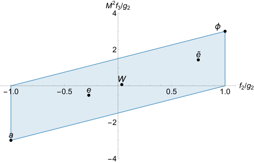
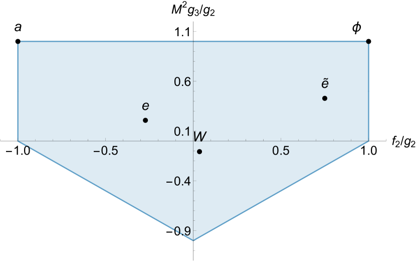
Figure 12: Allowed regions in the space $(M^{2}f_{3}/g_{2},f_{2}/g_{2})$ on the left, $(M^{2}g_{3}/g_{2},f_{2}/g_{2})$ on the right. They both give stronger bounds on the vertical direction w.r.t. Henriksson:2021ymi .

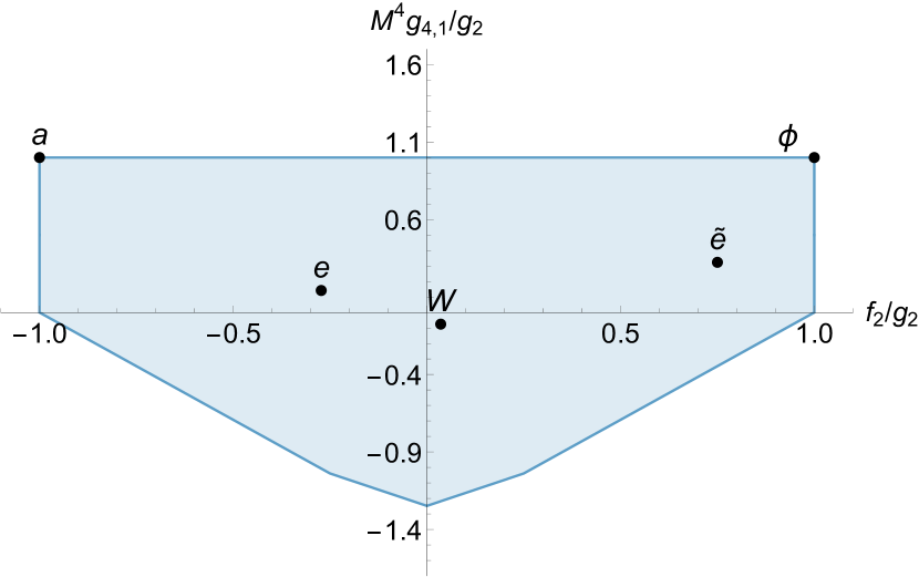
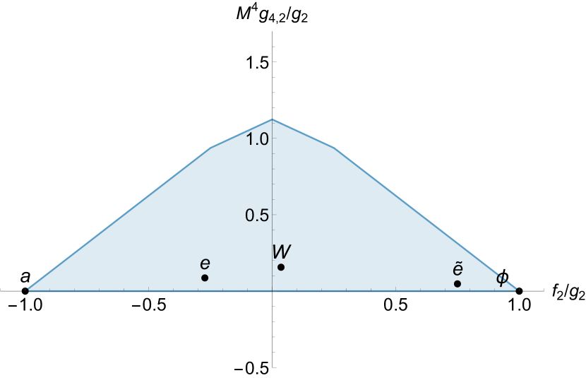
Figure 13: Allowed regions in the space $(M^{4}g_{4,1}/g_{2},f_{2}/g_{2})$ on the left, $(M^{4}g_{4,2}/g_{2},f_{2}/g_{2})$ on the right.

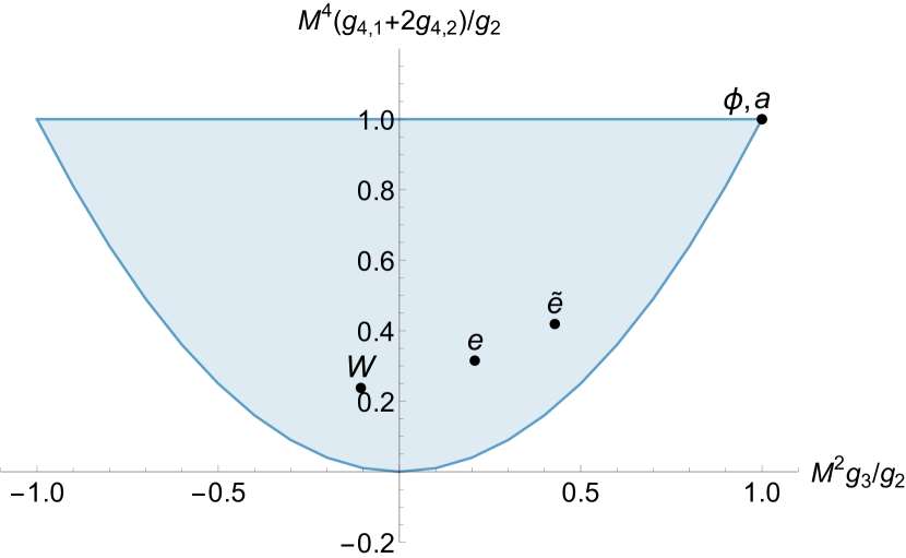
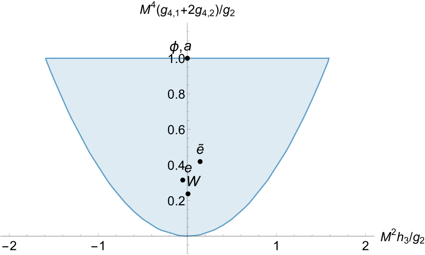
Figure 14: On the left, allowed region in the space $(M^{4}(g_{4,1}+2g_{4,2})/g_{2},M^{2}g_{3}/g_{2})$. We notice that it rules out a kink we were speculating about in Henriksson:2021ymi . On the right, a bound in the $(M^{4}(g_{4,1}+2g_{4,2})/g_{2},M^{2}h_{3}/g_{2})$ space.

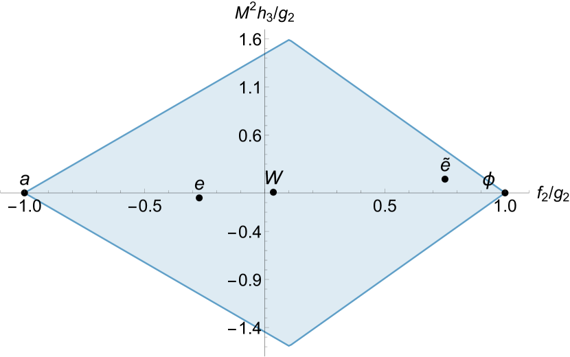
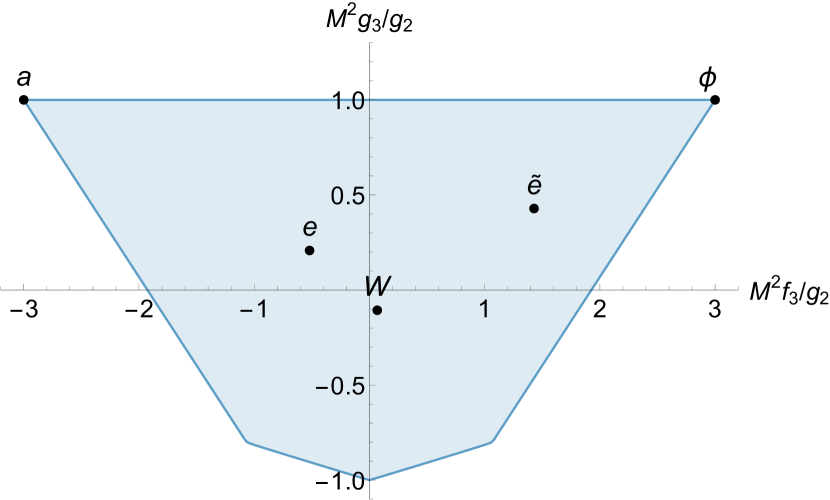
Figure 15: Allowed regions in the space $(M^{2}h_{3}/g_{2},f_{2}/g_{2})$ on the left, $(M^{2}g_{3}/g_{2},M^{2}f_{3}/g_{2})$ on the right.

Appendix C Details about numerical implementation

In this section we provide technical details about the numerical implementation of the algorithm discussed in section 3.1.1 in the main text. As discussed there, we need to impose positivity conditions (84) for all $m^{2}\geqslant M^{2}$ and on an infinite sequence of values of $\ell$. Let us discuss the various regimes, as outlined in figure 6 in section 3.1.2. All the parameters introduced in the following discussion are reported in table 4.

Table 4: Parameters used in the numerical implementation.

$\ell_{\text{max}}$	$m^{2}_{\text{max}}$	$B_{\text{max}}$	$\delta_{b}$	$\delta_{m}$	$\delta_{y}$	$n_{M}$	$n_{L}$	$n_{b}$	$n_{\text{max}}$
40	5	40	$10^{-2}$	$10^{-3}$	1/200	10	10	10	15/2

	non-standard SDPB parameter
precision	1024
dualityGapThreshold	$10^{-10}$
initialMatrixScaleDual	$10^{80}$
maxIteration	1000

1. Finite $m^{2}$, finite $\ell$: we impose positivity on the following set of spins:

   $$\ell\in\{0,2,3,4,5,\ldots,40,50,60,70,80,90,100,200\}\,.$$ (180)

   For each value of $\ell$, we include a discrete set of values for $m^{2}$:

   $$m^{2}\in\{M^{2},M^{2}+\delta_{m},M^{2}+2\delta_{m},\ldots,m^{2}_{\text{max}}\,\}\,.$$ (181)

   We checked that decreasing the interval of the discretization does not change the bounds substantially.

2. Large $m^{2}$, finite $\ell$: we computed a polynomial approximation of the high-energy part of the dispersion relation (81) integrated against $p^{n}$ for any $\ell$ as in (180). This is done by Taylor expanding these expressions around $m^{2}=\infty$ up to a certain order $n_{M}$, multiplying by the appropriate power of $m^{2}$ and substituting $m^{2}=m^{2}_{\text{max}}(1+x)$. The positivity condition is equivalent to the positivity of the resulting polynomial for any $x\geqslant 0$. This condition can be easily implemented in SDPB. We also checked that our approximation reproduces the original function to high precision for all $m\geqslant m_{\text{max}}$.

3. Finite $m^{2}$, large $\ell$: we computed a polynomial approximation of the high-energy part of the dispersion relation (81) integrated against $p^{n}$ for fixed values of $m^{2}$. This is done by Taylor expanding these expressions around $\ell=\infty$ up to a certain order $n_{L}$, multiplying by the appropriate power of $\ell$ and substituting $\ell=(500+x)$. Since we are interested in the large $\ell$ behavior, in all expressions (81), we can neglect hypergeometric functions, which are rapidly oscillating in this limit. We then require positivity of the resulting polynomial for any $x\geqslant 0$. The chosen values of $m^{2}$ are

   $$m^{2}=\frac{M^{2}}{1-y}\,,\quad\text{with}\quad y\in\{\delta_{y},2\delta_{y},\ldots,1-\delta_{y}\}\,.$$ (182)

4. Large $m^{2}$, large $\ell$, fixed $b=2\ell/m$: this limit is controlled by (93). We impose positivity on a discrete set of values of $b$:

   $$b\in\{\delta_{b},2\delta_{b},\ldots,B_{\text{max}}\}\,.$$ (183)

   To take into account the large $b$ regime, we Taylor expanded (93) around $b=\infty$ up to a certain order $n_{b}$ as in (97). Following Caron-Huot:2021rmr ; Caron-Huot:2022ugt , we rewrite an expression containing oscillating terms in terms of a $2\times 2$ matrix. For instance

   $$C_{0,n}(b)\simeq \frac{1}{b^{\frac{3}{2}+n_{b}}}\left(A_{n}(b)+B_{n}(b)\cos(b)+D_{n}(b)\sin(b)\right)$$ (184)

   $$\simeq \frac{1}{b^{\frac{3}{2}+n_{b}}}\begin{pmatrix}\cos(\frac{b}{2})&\sin(\frac{b}{2})\end{pmatrix}\cdot\begin{pmatrix}A_{n}(b)+B_{n}(b)&D_{n}(b)\\ D_{n}(b)&A_{n}(b)-B_{n}(b)\end{pmatrix}\cdot\begin{pmatrix}\cos(\frac{b}{2})\\ \sin(\frac{b}{2})\end{pmatrix}\,,$$

   where $A_{n},B_{n},D_{n}$ are polynomials in $b$. Given our choices of functional, they only contain integer powers of $b$. We then replace the positivity condition with the stronger requirement

   $$\sum a_{n}C_{0,n}(b)\geqslant 0\ \longrightarrow\ \sum a_{n}\begin{pmatrix}P^{(n)}_{1}(b)+P^{(n)}_{2}(b)&P^{(n)}_{3}(b)\\ P^{(n)}_{3}(b)&P^{(n)}_{1}(b)-P^{(n)}_{2}(b)\end{pmatrix}\succcurlyeq 0\,.$$ (185)

   A similar replacement can be done for any combination of $C_{\nu,n}(b)$. On the other hand the positivity conditions (84) also involve semi-definite conditions on linear combination of matrices. In the large $m^{2},\ell$ limit these matrices also contain oscillating terms, as shown in (93). Again we can replace each element of the matrices with a two by two matrix. For instance:

   $$\begin{pmatrix}C_{0,n}\\ 0&C_{0,n}\end{pmatrix}\rightarrow\begin{pmatrix}{\footnotesize\begin{pmatrix}A_{n}(b)+B_{n}(b)&D_{n}(b)\\ D_{n}(b)&A_{n}(b)-B_{n}(b)\end{pmatrix}}&{\footnotesize\begin{pmatrix}0&0\\ 0&0\end{pmatrix}}\\ {\footnotesize\begin{pmatrix}0&0\\ 0&0\end{pmatrix}}&{\footnotesize\begin{pmatrix}A_{n}(b)+B_{n}(b)&D_{n}(b)\\ D_{n}(b)&A_{n}(b)-B_{n}(b)\end{pmatrix}}\end{pmatrix},$$

   $$\begin{pmatrix}0&C_{2,n}\\ C_{2,n}&0\end{pmatrix}\rightarrow\begin{pmatrix}{\footnotesize\begin{pmatrix}0&0\\ 0&0\end{pmatrix}}&{\footnotesize\begin{pmatrix}A^{\prime}_{n}(b)+B^{\prime}_{n}(b)&D^{\prime}_{n}(b)\\ D^{\prime}_{n}(b)&A^{\prime}_{n}(b)-B^{\prime}_{n}(b)\end{pmatrix}}\\ {\footnotesize\begin{pmatrix}A^{\prime}_{n}(b)+B^{\prime}_{n}(b)&D^{\prime}_{n}(b)\\ D^{\prime}_{n}(b)&A^{\prime}_{n}(b)-B^{\prime}_{n}(b)\end{pmatrix}}&{\footnotesize\begin{pmatrix}0&0\\ 0&0\end{pmatrix}}\end{pmatrix}.$$ (186)

   We then demand positivity of linear combinations of the resulting $4\times 4$ matrices, which is again a stronger condition but has the advantage of being in the form of a polynomial matrix, which can be fed to SDPB.

Finally, let us list the procedures followed to obtain each figure:

• Figure 5: we used the dispersion relations $\mathcal{I}_{g},\mathcal{I}_{0}$ and $\mathcal{I}_{\beta^{2}}$. This is equivalent to considering $\Lambda[\vec{v}]=\sum_{i}\Lambda_{i}[v_{i}]$, with $i=1,4,5$. The low-energy part only depends on $g_{2}$ and $\beta$. Just as we did in section 3.2.2, obtained bounds along rays in the $(g_{2},\beta^{2})$ plane: we looked for a functional satisfying (see (75))

  $$\frac{1}{M^{4}}\cos\theta\Lambda_{1}[1]+\frac{M^{2}_{\textrm{P}}}{M^{6}}\sin\theta\left(\Lambda_{1}[4p^{2}]-\Lambda_{5}[p^{2}]\right)=1\,,$$ (187)

  $$\text{maximize}\quad-\Lambda_{1}[p^{-2}]\,.$$ (188)

• Figure 10: we used the dispersion relations $\mathcal{I}_{g},\mathcal{I}_{f},\mathcal{I}_{0}$ and $I_{\beta^{2}}$. This is equivalent to considering $\Lambda[\vec{v}]=\sum_{i}\Lambda_{i}[v_{i}]$, with $i=1,2,4,5$. The low-energy part only depends on $g_{2}$, $\beta$, $f_{2}$ and $f_{3}$. This time we obtained bounds along rays in the $(g_{2},f_{2})$ plane while leaving $\beta^{2}$ and $f_{3}$ undetermined. Hence we looked for a functional satisfying (see (75))

  $$\frac{1}{M^{4}}\cos\theta\Lambda_{1}[1]+\frac{1}{M^{4}}\sin\theta\Lambda_{2}[1]=1\,,$$ (189)

  $$-\left(\Lambda_{1}[4p^{2}]+5\Lambda_{2}[p^{2}]-\Lambda_{5}[p^{2}]\right)\geqslant 0\,,$$ (190)

  $$\pm\Lambda_{2}[p^{2}]\geqslant 0\,,$$ (191)

  $$\text{maximize}\quad-\Lambda_{1}[p^{-2}]\,.$$ (192)

  The second and third condition ensures that we can discard the contribution of $\beta^{2}$ and $f_{3}$, provided that the latter has fixed sign. Hence the two distinct allowed regions. The overall allowed region is the union of the two regions.

• Figure 11: we used the dispersion relations $\mathcal{I}_{g},\mathcal{I}_{h},\mathcal{I}_{0}$ and $\mathcal{I}_{\beta^{2}}$. This is equivalent to considering $\Lambda[\vec{v}]=\sum_{i}\Lambda_{i}[v_{i}]$, with $i=1,3,4,5$. The low-energy part only depends on $g_{2}$, $\beta$, $\beta$ and $h_{3}$. This time we cannot get bounds along rays since both $\beta$ and $\beta^{2}$ appear. Hence we scanned over $\beta$, and got bounds on $g_{2}$. We looked for a functional satisfying (see (75))

  $$\Lambda_{1}[1]=1\,,$$ (193)

  $$\pm\Lambda_{3}[p^{2}]\geqslant 0\,,$$ (194)

  $$\text{maximize}-\left(\Lambda_{1}[p^{-2}]+\beta^{2}\left(\Lambda_{1}[4p^{2}]-\Lambda_{5}[p^{2}]\right)+\beta\Lambda_{3}[1]\right)\,.$$ (195)

  The second condition ensures that we can discard the contribution of $h_{3}$, provided that it has fixed sign. It turns out that the allowed region is independent of the choice of the sign.

References

- (1) T.N. Pham and T.N. Truong, Evaluation of the derivative quartic terms of the meson chiral Lagrangian from forward dispersion relation, Phys. Rev. D 31 (1985) 3027.
- (2) M.R. Pennington and J. Portoles, The Chiral Lagrangian parameters, , , are determined by the -resonance, Phys. Lett. B 344 (1995) 399 [hep-ph/9409426].
- (3) B. Ananthanarayan, D. Toublan and G. Wanders, Consistency of the chiral pion pion scattering amplitudes with axiomatic constraints, Phys. Rev. D 51 (1995) 1093 [hep-ph/9410302].
- (4) J. Comellas, J.I. Latorre and J. Taron, Constraints on chiral perturbation theory parameters from QCD inequalities, Phys. Lett. B 360 (1995) 109 [hep-ph/9507258].
- (5) P. Dita, Positivity constraints on chiral perturbation theory pion pion scattering amplitudes, Phys. Rev. D 59 (1999) 094007 [hep-ph/9809568].
- (6) A. Adams, N. Arkani-Hamed, S. Dubovsky, A. Nicolis and R. Rattazzi, Causality, analyticity and an IR obstruction to UV completion, JHEP 10 (2006) 014 [hep-th/0602178].
- (7) A.V. Manohar and V. Mateu, Dispersion relation bounds for pi pi scattering, Phys. Rev. D 77 (2008) 094019 [0801.3222].
- (8) V. Mateu, Universal bounds for low energy constants, Phys. Rev. D 77 (2008) 094020 [0801.3627].
- (9) A. Nicolis, R. Rattazzi and E. Trincherini, Energy’s and amplitudes’ positivity, JHEP 05 (2010) 095 [0912.4258]. [Erratum: JHEP 11 (2011) 128].
- (10) D. Baumann, D. Green, H. Lee and R.A. Porto, Signs of analyticity in single-field inflation, Phys. Rev. D 93 (2016) 023523 [1502.07304].
- (11) B. Bellazzini, C. Cheung and G.N. Remmen, Quantum gravity constraints from unitarity and analyticity, Phys. Rev. D 93 (2016) 064076 [1509.00851].
- (12) B. Bellazzini, Softness and amplitudes’ positivity for spinning particles, JHEP 02 (2017) 034 [1605.06111].
- (13) C. Cheung and G.N. Remmen, Positive signs in massive gravity, JHEP 04 (2016) 002 [1601.04068].
- (14) J. Bonifacio, K. Hinterbichler and R.A. Rosen, Positivity constraints for pseudolinear massive spin-2 and vector Galileons, Phys. Rev. D 94 (2016) 104001 [1607.06084].
- (15) C. Cheung and G.N. Remmen, Positivity of curvature-squared corrections in gravity, Phys. Rev. Lett. 118 (2017) 051601 [1608.02942].
- (16) C. de Rham, S. Melville, A.J. Tolley and S.-Y. Zhou, Positivity bounds for scalar field theories, Phys. Rev. D 96 (2017) 081702 [1702.06134].
- (17) B. Bellazzini, F. Riva, J. Serra and F. Sgarlata, Beyond positivity bounds and the fate of massive gravity, Phys. Rev. Lett. 120 (2018) 161101 [1710.02539].
- (18) C. de Rham, S. Melville, A.J. Tolley and S.-Y. Zhou, UV complete me: Positivity bounds for particles with spin, JHEP 03 (2018) 011 [1706.02712].
- (19) C. de Rham, S. Melville, A.J. Tolley and S.-Y. Zhou, Massive Galileon positivity bounds, JHEP 09 (2017) 072 [1702.08577].
- (20) K. Hinterbichler, A. Joyce and R.A. Rosen, Massive spin-2 scattering and asymptotic superluminality, JHEP 03 (2018) 051 [1708.05716].
- (21) J. Bonifacio, K. Hinterbichler, A. Joyce and R.A. Rosen, Massive and massless spin-2 scattering and asymptotic superluminality, JHEP 06 (2018) 075 [1712.10020].
- (22) B. Bellazzini, F. Riva, J. Serra and F. Sgarlata, The other effective fermion compositeness, JHEP 11 (2017) 020 [1706.03070].
- (23) J. Bonifacio and K. Hinterbichler, Bounds on amplitudes in effective theories with massive spinning particles, Phys. Rev. D 98 (2018) 045003 [1804.08686].
- (24) C. de Rham, S. Melville, A.J. Tolley and S.-Y. Zhou, Positivity bounds for massive spin-1 and spin-2 fields, JHEP 03 (2019) 182 [1804.10624].
- (25) C. Zhang and S.-Y. Zhou, Positivity bounds on vector boson scattering at the LHC, Phys. Rev. D 100 (2019) 095003 [1808.00010].
- (26) B. Bellazzini and F. Riva, New phenomenological and theoretical perspective on anomalous ZZ and Z processes, Phys. Rev. D 98 (2018) 095021 [1806.09640].
- (27) B. Bellazzini, M. Lewandowski and J. Serra, Positivity of amplitudes, weak gravity conjecture, and modified gravity, Phys. Rev. Lett. 123 (2019) 251103 [1902.03250].
- (28) S. Melville and J. Noller, Positivity in the sky: Constraining dark energy and modified gravity from the UV, Phys. Rev. D 101 (2020) 021502 [1904.05874]. [Erratum: Phys. Rev. D 102 (2020) 049902].
- (29) C. de Rham and A.J. Tolley, Speed of gravity, Phys. Rev. D 101 (2020) 063518 [1909.00881].
- (30) L. Alberte, C. de Rham, A. Momeni, J. Rumbutis and A.J. Tolley, Positivity constraints on interacting spin-2 fields, JHEP 03 (2020) 097 [1910.11799].
- (31) L. Alberte, C. de Rham, A. Momeni, J. Rumbutis and A.J. Tolley, Positivity constraints on interacting pseudo-linear spin-2 fields, JHEP 07 (2020) 121 [1912.10018].
- (32) Q. Bi, C. Zhang and S.-Y. Zhou, Positivity constraints on aQGC: carving out the physical parameter space, JHEP 06 (2019) 137 [1902.08977].
- (33) G.N. Remmen and N.L. Rodd, Consistency of the Standard Model Effective Field Theory, JHEP 12 (2019) 032 [1908.09845].
- (34) G. Ye and Y.-S. Piao, Positivity in the effective field theory of cosmological perturbations, Eur. Phys. J. C 80 (2020) 421 [1908.08644].
- (35) M. Herrero-Valea, I. Timiryasov and A. Tokareva, To positivity and beyond, where Higgs-dilaton inflation has never gone before, JCAP 11 (2019) 042 [1905.08816].
- (36) C. Zhang and S.-Y. Zhou, Convex geometry perspective on the (Standard Model) Effective Field Theory Space, Phys. Rev. Lett. 125 (2020) 201601 [2005.03047].
- (37) N. Arkani-Hamed, T.-C. Huang and Y.-T. Huang, The EFT-hedron, JHEP 05 (2021) 259 [2012.15849].
- (38) B. Bellazzini, J. Elias Miró, R. Rattazzi, M. Riembau and F. Riva, Positive moments for scattering amplitudes, Phys. Rev. D 104 (2021) 036006 [2011.00037].
- (39) A.J. Tolley, Z.-Y. Wang and S.-Y. Zhou, New positivity bounds from full crossing symmetry, JHEP 05 (2021) 255 [2011.02400].
- (40) S. Caron-Huot and V. Van Duong, Extremal effective field theories, JHEP 05 (2021) 280 [2011.02957].
- (41) A. Sinha and A. Zahed, Crossing symmetric dispersion relations in quantum field theories, Phys. Rev. Lett. 126 (2021) 181601 [2012.04877].
- (42) T. Trott, Causality, unitarity and symmetry in effective field theory, JHEP 07 (2021) 143 [2011.10058].
- (43) C. Zhang, SMEFTs living on the edge: determining the UV theories from positivity and extremality, 2112.11665.
- (44) Y.-J. Wang, F.-K. Guo, C. Zhang and S.-Y. Zhou, Generalized positivity bounds on chiral perturbation theory, JHEP 07 (2020) 214 [2004.03992].
- (45) X. Li, H. Xu, C. Yang, C. Zhang and S.-Y. Zhou, Positivity in multifield effective field theories, Phys. Rev. Lett. 127 (2021) 121601 [2101.01191].
- (46) Z.-Z. Du, C. Zhang and S.-Y. Zhou, Triple crossing positivity bounds for multi-field theories, JHEP 12 (2021) 115 [2111.01169].
- (47) J. Davighi, S. Melville and T. You, Natural selection rules: new positivity bounds for massive spinning particles, JHEP 02 (2022) 167 [2108.06334].
- (48) S.D. Chowdhury, K. Ghosh, P. Haldar, P. Raman and A. Sinha, Crossing symmetric spinning S-matrix bootstrap: EFT bounds, 2112.11755.
- (49) J. Henriksson, B. McPeak, F. Russo and A. Vichi, Rigorous bounds on light-by-light scattering, 2107.13009.
- (50) Z. Bern, D. Kosmopoulos and A. Zhiboedov, Gravitational effective field theory islands, low-spin dominance, and the four-graviton amplitude, J. Phys. A 54 (2021) 344002 [2103.12728].
- (51) C. de Rham, S. Kundu, M. Reece, A.J. Tolley and S.-Y. Zhou, Snowmass White Paper: UV constraints on IR physics, 2022 [2203.06805].
- (52) N. Arkani-Hamed, L. Motl, A. Nicolis and C. Vafa, The string landscape, black holes and gravity as the weakest force, JHEP 06 (2007) 060 [hep-th/0601001].
- (53) Y. Kats, L. Motl and M. Padi, Higher-order corrections to mass-charge relation of extremal black holes, JHEP 12 (2007) 068 [hep-th/0606100].
- (54) C. Cheung and G.N. Remmen, Infrared consistency and the weak gravity conjecture, JHEP 12 (2014) 087 [1407.7865].
- (55) Y. Hamada, T. Noumi and G. Shiu, Weak gravity conjecture from unitarity and causality, Phys. Rev. Lett. 123 (2019) 051601 [1810.03637].
- (56) L. Alberte, C. de Rham, S. Jaitly and A.J. Tolley, Positivity bounds and the massless spin-2 pole, Phys. Rev. D 102 (2020) 125023 [2007.12667].
- (57) L. Alberte, C. de Rham, S. Jaitly and A.J. Tolley, QED positivity bounds, Phys. Rev. D 103 (2021) 125020 [2012.05798].
- (58) T.J. Hollowood and G.M. Shore, Causality violation, gravitational shockwaves and UV completion, JHEP 03 (2016) 129 [1512.04952].
- (59) C. de Rham and A.J. Tolley, Causality in curved spacetimes: The speed of light and gravity, Phys. Rev. D 102 (2020) 084048 [2007.01847].
- (60) I.T. Drummond and S.J. Hathrell, QED vacuum polarization in a background gravitational field and its effect on the velocity of photons, Phys. Rev. D 22 (1980) 343.
- (61) G. Goon and K. Hinterbichler, Superluminality, black holes and EFT, JHEP 02 (2017) 134 [1609.00723].
- (62) X.O. Camanho, J.D. Edelstein, J. Maldacena and A. Zhiboedov, Causality constraints on corrections to the graviton three-point coupling, JHEP 02 (2016) 020 [1407.5597].
- (63) B. Bellazzini, Softness, Amplitudes’ positivity & EFT for Spinning Particles, . Talk given at Utrecht joint Cosmoslogy and Holography meeting.
- (64) A. Falkowski, Saclay lectures on effective field theories, . Lectures Notes for Saclay 2017.
- (65) S. Caron-Huot, D. Mazac, L. Rastelli and D. Simmons-Duffin, Sharp boundaries for the Swampland, JHEP 07 (2021) 110 [2102.08951].
- (66) S. Caron-Huot, Y.-Z. Li, J. Parra-Martinez and D. Simmons-Duffin, Causality constraints on corrections to Einstein gravity, 2201.06602.
- (67) D. Harlow, B. Heidenreich, M. Reece and T. Rudelius, The Weak Gravity Conjecture: A review, 2201.08380.
- (68) T. Banks, M. Johnson and A. Shomer, A note on gauge theories coupled to gravity, JHEP 09 (2006) 049 [hep-th/0606277].
- (69) L. Susskind, Trouble for remnants, hep-th/9501106.
- (70) T. Banks and N. Seiberg, Symmetries and strings in field theory and gravity, Phys. Rev. D 83 (2011) 084019 [1011.5120].
- (71) D. Harlow and H. Ooguri, Symmetries in quantum field theory and quantum gravity, Commun. Math. Phys. 383 (2021) 1669 [1810.05338].
- (72) C.R.T. Jones and B. McPeak, The Black Hole Weak Gravity Conjecture with multiple charges, JHEP 06 (2020) 140 [1908.10452].
- (73) M. Froissart, Asymptotic behavior and subtractions in the Mandelstam representation, Phys. Rev. 123 (1961) 1053.
- (74) A. Martin, Extension of the axiomatic analyticity domain of scattering amplitudes by unitarity. 1., Nuovo Cim. A 42 (1965) 930.
- (75) S.D. Chowdhury, A. Gadde, T. Gopalka, I. Halder, L. Janagal and S. Minwalla, Classifying and constraining local four photon and four graviton S-matrices, JHEP 02 (2020) 114 [1910.14392].
- (76) K. Häring and A. Zhiboedov, Gravitational Regge bounds, 2202.08280.
- (77) M. Jacob and G.C. Wick, On the general theory of collisions for particles with spin, Annals Phys. 7 (1959) 404.
- (78) A. Hebbar, D. Karateev and J. Penedones, Spinning S-matrix bootstrap in 4d, JHEP 01 (2022) 060 [2011.11708].
- (79) M.D. Thorsley and M.C. Chidichimo, An asymptotic expansion for the hypergeometric function , J. Math. Phys. 42 (2001) 1921.
- (80) G.N. Watson, A Treatise on the Theory of Bessel Functions, 2nd ed., Cambridge University Press (1944).
- (81) D. Simmons-Duffin, A semidefinite program solver for the conformal bootstrap, JHEP 06 (2015) 174 [1502.02033].
- (82) W. Landry and D. Simmons-Duffin, Scaling the semidefinite program solver SDPB, 1909.09745.
- (83) G. Dvali, Black holes and large species solution to the hierarchy problem, Fortsch. Phys. 58 (2010) 528 [0706.2050].
- (84) G. Dvali and M. Redi, Black hole bound on the number of species and quantum gravity at LHC, Phys. Rev. D 77 (2008) 045027 [0710.4344].
- (85) P.P. Kulish and L.D. Faddeev, Asymptotic conditions and infrared divergences in quantum electrodynamics, Theor. Math. Phys. 4 (1970) 745.
- (86) S. Caron-Huot, D. Mazac, L. Rastelli and D. Simmons-Duffin, AdS bulk locality from sharp CFT bounds, JHEP 11 (2021) 164 [2106.10274].
- (87) S. Cremonini, C.R.T. Jones, J.T. Liu and B. McPeak, Higher-derivative corrections to entropy and the Weak Gravity Conjecture in anti-de Sitter space, JHEP 09 (2020) 003 [1912.11161].
- (88) P.A. Cano, A. Murcia, A.R. Sánchez and X. Zhang, Higher-derivative holography with a chemical potential, 2202.10473.
- (89) D. Li, D. Meltzer and D. Poland, Conformal bootstrap in the Regge limit, JHEP 12 (2017) 013 [1705.03453].
- (90) N. Afkhami-Jeddi, S. Kundu and A. Tajdini, A conformal collider for holographic CFTs, JHEP 10 (2018) 156 [1805.07393].
- (91) J.D. Bekenstein, Black holes and entropy, Phys. Rev. D 7 (1973) 2333.
- (92) J.D. Bekenstein, Generalized second law of thermodynamics in black hole physics, Phys. Rev. D 9 (1974) 3292.
- (93) J.D. Bekenstein, A universal upper bound on the entropy to energy ratio for bounded systems, Phys. Rev. D 23 (1981) 287.
- (94) A.G. Cohen, D.B. Kaplan and A.E. Nelson, Effective field theory, black holes, and the cosmological constant, Phys. Rev. Lett. 82 (1999) 4971 [hep-th/9803132].
- (95) S. Cremonini, C.R.T. Jones, J.T. Liu, B. McPeak and Y. Tang, NUT charge weak gravity conjecture from dimensional reduction, Phys. Rev. D 103 (2021) 106011 [2011.06083].
- (96) P. Kovtun, D.T. Son and A.O. Starinets, Viscosity in strongly interacting quantum field theories from black hole physics, Phys. Rev. Lett. 94 (2005) 111601 [hep-th/0405231].
- (97) S. Cremonini, The shear viscosity to entropy ratio: A status report, Mod. Phys. Lett. B 25 (2011) 1867 [1108.0677].