New tests of dark sector interactions from the full-shape galaxy power spectrum
Abstract
We explore the role of redshift-space galaxy clustering data in constraining non-gravitational interactions between dark energy (DE) and dark matter (DM), for which state-of-the-art limits have so far been obtained from late-time background measurements. We use the joint likelihood for pre-reconstruction full-shape (FS) galaxy power spectrum and post-reconstruction Baryon Acoustic Oscillation (BAO) measurements from the BOSS DR12 sample, alongside Cosmic Microwave Background (CMB) data from Planck: from this dataset combination we infer and the 2 lower limit , among the strongest limits ever reported on the DM-DE coupling strength for the particular model considered. Contrary to what has been observed for the CDM model and simple extensions thereof, we find that the CMB+FS combination returns tighter constraints compared to the CMB+BAO one, suggesting that there is valuable additional information contained in the broadband of the power spectrum. We test this finding by running additional CMB-free analyses and removing sound horizon information, and discuss the important role of the equality scale in setting constraints on DM-DE interactions. Our results reinforce the critical role played by redshift-space galaxy clustering measurements in the epoch of precision cosmology, particularly in relation to tests of non-minimal dark sector extensions of the CDM model.
I Introduction
Dark energy (DE) accounts for approximately of the Universe’s energy budget, yet its nature remains puzzling. Within the standard six-parameter CDM cosmological model, DE takes the form of a smooth, time-independent, spatially uniform vacuum energy component. This simple model is able to provide an extremely good fit to a wide variety of cosmological and astrophysical observations, including anisotropies in the Cosmic Microwave Background (CMB), the clustering of the large-scale structure (LSS), the magnitude-redshift relation of Type Ia Supernovae (SNeIa) in the Hubble flow, the distortion of images of distant galaxies due to weak lensing from the intervening LSS (cosmic shear), and the abundances of light elements Riess et al. (1998); Perlmutter et al. (1999); Aghanim et al. (2020a); Aiola et al. (2020); Alam et al. (2021); Asgari et al. (2021); Mossa et al. (2020); Dutcher et al. (2021); Abbott et al. (2022); Scolnic et al. (2021).
Of course, this very economical picture does not need to be the end of the story as far as DE is concerned. One reason for this belief is the (in)famous cosmological constant problem Weinberg (1989). In an attempt to construct more realistic physical models for DE, significant effort has been placed into going beyond the minimal scenario. Examples include models endowing DE with a dynamical nature Wetterich (1988); Ratra and Peebles (1988); Caldwell et al. (1998), or featuring non-trivial interactions between DE and other components of the Universe’s energy budget. Examples of the latter are interacting DE (IDE) models, which exhibit interactions between dark matter (DM) and DE, historically motivated by attempts to address the coincidence problem Zlatev et al. (1999); Huey and Wandelt (2006); Velten et al. (2014).111However, the amount of energy exchange required to address this problem is now excluded by observations. See in addition Refs. D’Amico et al. (2016); Marsh (2017) for further issues which have been raised in this context owing to quantum corrections.
State-of-the-art constraints on IDE cosmologies arise primarily from measurements of temperature and polarization anisotropies in the CMB, in combination with measurements of the late-time background expansion history from BAO and Hubble flow SNeIa. In combination, these probes have set stringent constraints on the strength of the DM-DE interaction, typically denoted by : the constraints depend on the specific assumptions concerning the form of the interaction, and on the datasets adopted, but typically restrict (see e.g. Refs. Di Valentino et al. (2017); Yang et al. (2019a); Cheng et al. (2020); Yang et al. (2020a, 2021a) for some of the latest constraints, see also Refs. Zhang et al. (2019, 2018); Liu et al. (2022)). Incidentally, these tight constraints from BAO and SNeIa are the key reason why IDE scenarios fall short of fully addressing the Hubble tension Bernal et al. (2016); Addison et al. (2018); Mörtsell and Dhawan (2018); Lemos et al. (2019); Aylor et al. (2019); Knox and Millea (2020); Arendse et al. (2020); Zhang and Huang (2021); Efstathiou (2021); Cai et al. (2022), despite these models having experienced somewhat of a revival in recent years in attempts to address cosmological tensions (see e.g. Refs. Di Valentino et al. (2021a, b); Perivolaropoulos and Skara (2021); Schöneberg et al. (2021); Abdalla et al. (2022) for reviews on the Hubble tension).
In recent years, significant efforts have gone into extracting LSS clustering information beyond that contained within the (reconstructed) BAO peaks, using information from the full-shape (FS) power spectrum of biased tracers of the LSS. These efforts have been driven in part by significant advances in the so-called Effective Field Theory of LSS (EFTofLSS) Baumann et al. (2012), which have allowed for concrete applications of this framework to real data from galaxy redshift surveys: these advances motivate us to re-analyze IDE models in this context. It is our major goal in the present work to explore whether redshift-space galaxy clustering data can improve state-of-the-art constraints on the DM-DE interaction strength.222We note that the same interacting DE model that will be examined in this work had actually been confronted against FS galaxy power spectrum measurements by one of us in 2009 in Ref. Gavela et al. (2009). However, this early study was performed using the FS power spectrum of luminous red galaxies from the Sloan Digital Sky Survey (SDSS) Data Release 4 (DR4) sample, alongside CMB and SNeIa measurements from WMAP and the Union dataset. All these datasets are now significantly outdated, and the modeling of the FS galaxy power spectrum was significantly simplified. Therefore it is extremely timely to re-examine this issue nearly 15 years later, making use of state-of-the-art cosmological measurements, in combination with a more robust theoretical modeling of the FS galaxy power spectrum. See also the later Ref. Duniya et al. (2015) for an investigation of horizon-scale relativistic effects in the galaxy power spectrum in the presence of interacting DE.
The rest of this paper is then organized as follows. In Sec. II, we review the physics of IDE models, present the specific model we will study, before briefly discussing the EFTofLSS and how our model fits within this framework. In Sec. III we discuss the datasets and analysis methodology we make use of. The results of this analysis are presented in Sec. IV. Finally, in Sec. V we provide our concluding remarks.
II Dark sector interactions and the full-shape galaxy power spectrum
II.1 Interacting dark energy
We begin by reviewing the basic features of IDE models. In the following, we shall work under the assumption of a spatially flat Friedmann-Lemaître-Robertson-Walker metric. In the absence of DM-DE interactions the stress-energy tensors of DM and DE, which we denote by and respectively, are separately covariantly conserved. This implies:
| (1) |
where denotes the covariant derivative. However, particularly in the case where DE is described by a new light field (as in quintessence models), couplings of DE to matter fields (typically with gravitational strength) are somewhat unavoidable, unless protected by a specific symmetry Carroll (1998). When introducing non-gravitational interactions between DM and DE, there are essentially two ways to proceed. One can either work from first principles in the context of a specific (possibly UV-complete) model, where the interaction between the dark components is introduced at the level of the action. Historically, this was in fact the approach first followed, particularly in the context of so-called coupled quintessence models, where a light quintessence DE field is coupled to the DM field Wetterich (1995); Amendola (2000a, b); Mangano et al. (2003); Farrar and Peebles (2004). Alternatively, one can introduce a phenomenological parametrization for the DM-DE interaction at the level of the conservation equations in Eq. (1), in such a way that the two stress-energy tensors are separately not conserved, but their sum is. In this work, we shall follow the second approach.333We note that a separate but nonetheless associated possibility recently considered in the literature is that where DE interacts either with baryons Vagnozzi et al. (2020); Jiménez et al. (2020); Vagnozzi et al. (2021a); Benisty and Davis (2022); Ferlito et al. (2022) or with electromagnetism Calabrese et al. (2014); Martins and Pinho (2015); Martins et al. (2015, 2016); Martinelli et al. (2021). See also Refs. He and Zhang (2017); Zhang (2022) for works discussing the related possibility of direct detection of DE. Typically, one assumes that the covariant derivatives of the DM and DE stress-energy tensors evolve as:
| (2) | |||||
| (3) |
where is the DM velocity 4-vector, and is the DM-DE interaction rate (with units of energy per volume per time). At this point, one needs to make a (phenomenological) choice for the functional form of . A choice commonly adopted in the literature is the following:
| (4) |
where is the conformal Hubble rate, is the DE energy density and is a dimensionless parameter which controls the strength of the DM-DE interaction: a value of () indicates energy transfer from the DE (DM) to the DM (DE) sector.
A comment is in order regarding the appearance of in the interaction rate. This might appear puzzling at first, as it may suggest that an interaction rate which should ultimately be determined by local interactions is actually sensitive to a global quantity such as the expansion rate, see e.g. Ref. Valiviita et al. (2008). In reality, the appearance of is ultimately a consequence of the first principle of thermodynamics, a local law (independently of the context to which one applies it, for example cosmology) which essentially states that changes in the density respond to changes in the volume due to cosmic expansion. In other words, the conservation equations do not explicitly know about the underlying cosmology or theory of gravity, but only about the change in scale or volume. In fact, one can eliminate entirely and use the scale factor as time variable (as in the non-interacting case).444We thank the anonymous referee of one of our previous papers for drawing our attention to this issue, whereas S.V. thanks Marco Bruni for sharing this illuminating explanation. In addition, we note that Ref. Pan et al. (2020) explicitly showed how interaction rates featuring factors related to , including but not limited to the case considered in Eq. (4), may naturally emerge from first principles when considering well-motivated field theories for IDE scenarios.
In the presence of the coupling given by Eq. (4), the continuity equations for the DM and DE energy densities and are modified to:
| (5) | |||||
| (6) |
where is the DE equation of state (EoS). Assuming that both ad are constant in cosmic time, the above Eqs. (5,6) can be analytically integrated to give:
| (7) | |||||
| (8) |
where and are the present-day energy densities of DM and DE. From Eq. (8), we see that in the presence of such an interaction the DE component effectively behaves as a component with EoS .
The presence of the DM-DE coupling also modifies the evolution of perturbations. Working in synchronous gauge, the coupled system of linear Einstein-Boltzmann equations for the evolution of the DM and DE density perturbations ( and ) and velocity divergences ( and ) is given by Valiviita et al. (2008); Gavela et al. (2010); Lopez Honorez et al. (2010):
| (9) | |||||
| (10) | |||||
| (11) | |||||
| (12) |
where we set the DE sound speed squared to , and and refer to the trace of the metric perturbation in the synchronous gauge and to the center of mass velocity for the total fluid respectively, where the appearance of the latter is required by gauge invariance arguments Gavela et al. (2010). The initial conditions for the DE density perturbation and velocity divergence are also modified, following Ref. Gavela et al. (2010).
Furthermore, one needs to avoid instabilities in the system of Eqs. (9–12). Gravitational and non-adiabatic (early-time) instabilities can be avoided provided that a) , and b) and carry opposite signs Gavela et al. (2009, 2010). In this work, our goal will be that of examining a scenario which is as close as possible to that of an interacting vacuum, where . This is strictly speaking not possible, due to gravitational instabilities. However, here we will opt for the phenomenological choice of setting to a small but non-zero value. Specifically, we fix , thus requiring . The rationale behind this approach is that, for sufficiently small, the effect of the DE perturbations is negligible at the level of the coupled Einstein-Boltzmann system, which are instead essentially only capturing the effect of the DM-DE interaction governed by . This was explicitly demonstrated by one of us through simulated data in Ref. Di Valentino and Mena (2020).555In principle, we could equally well have opted for the choice of setting and . However, there are at least two good reasons to not consider this possibility. The first is that quintessence-like DE scenarios where are actually theoretically more motivated (or at least theoretically easier to come about) compared to phantom scenarios where . The second is that a scenario where energy flows from the DM to the DE () is somewhat theoretically more natural than the reverse case (). Note, however, that the simplest quintessence models appear on their own to be observationally disfavored, as they worsen the tension Banerjee et al. (2021). We note that such an approach has already been followed in several previous works, see e.g. Refs. Di Valentino et al. (2020a, b); Lucca and Hooper (2020). We also note that another approach towards avoiding gravitational instabilities, investigated in Refs. Li et al. (2014a, b); Guo et al. (2017); Zhang (2017); Guo et al. (2018a), is to extend the parameterized post-Friedmann approach to the IDE case.
In closing, it is worth noting that IDE models have received significant attention in recent years. For a selection of important works on various aspects of IDE models besides those already discussed, ranging from model-building to structure formation simulations to observational constraints, we refer the reader to Refs. Amendola and Quercellini (2003); Pettorino et al. (2005a, b); Barrow and Clifton (2006); Bean et al. (2008); He and Wang (2008); Pettorino and Baccigalupi (2008); Baldi et al. (2010); Majerotto et al. (2010); Jamil et al. (2010); Martinelli et al. (2010); Baldi and Pettorino (2011); De Bernardis et al. (2011); Baldi (2012); Pettorino et al. (2012); Carbone et al. (2013); Piloyan et al. (2013); Pettorino (2013); Pourtsidou et al. (2013); Piloyan et al. (2014); Faraoni et al. (2014); Ferreira et al. (2017); Ade et al. (2016); Skordis et al. (2015); Tamanini (2015); Marra (2016); Murgia et al. (2016); Pourtsidou and Tram (2016); Nunes et al. (2016); Kumar and Nunes (2016, 2017a); Benisty and Guendelman (2017); Yang et al. (2018a); Mifsud and Van De Bruck (2017); Yang et al. (2017); Kumar and Nunes (2017b); Guo et al. (2018b); Dutta et al. (2018); Feng et al. (2019); Benisty and Guendelman (2018); Barros et al. (2019); Costa et al. (2018); Yang et al. (2018b); von Marttens et al. (2019a); Elizalde et al. (2018); Guo et al. (2019); Yang et al. (2018c); Li et al. (2019); von Marttens et al. (2019b); Cárdenas et al. (2019); Benisty et al. (2019); Bonici and Maggiore (2019); Martinelli et al. (2019); Kumar et al. (2019); Pan et al. (2019a); Li et al. (2020); Yang et al. (2019b); Pan et al. (2019b); Landim (2019); Benetti et al. (2019); von Marttens et al. (2020); Kase and Tsujikawa (2020); Liu et al. (2020); Yang et al. (2020b); Chamings et al. (2020); Sharma and Dubey (2022); Yang et al. (2020c); Hogg et al. (2020); Amendola and Tsujikawa (2020); Benisty et al. (2020); Gómez-Valent et al. (2020); Aljaf et al. (2021); Di Valentino et al. (2020c); Mukhopadhyay et al. (2021); Di Valentino (2021); Di Valentino et al. (2021c); Yao and Meng (2021); Beltrán Jiménez et al. (2021); Yang et al. (2021b); Sinha (2021); Gao et al. (2021); Zhang et al. (2021); Salzano et al. (2021); Wang et al. (2021); Benetti et al. (2021); Kumar (2021); Figueruelo et al. (2021); Bora et al. (2021); Jiménez et al. (2021); Carrilho et al. (2021a); Lucca (2021a); Bora et al. (2022); Linton et al. (2021); Nunes and Di Valentino (2021); Anchordoqui et al. (2021); Hogg and Bruni (2022); Guo et al. (2021); Alestas et al. (2021); Mancini and Pourtsidou (2022); Gariazzo et al. (2021); Carrilho et al. (2021b); Sharma and Sur (2021); Duniya (2022) and to the review of Ref. Wang et al. (2016).
II.2 Interacting dark energy and the Effective Field Theory of Large-Scale Structure
There is a wealth of information contained in the linear and mildly non-linear clustering of tracers of the LSS, such as galaxies, on which our analysis will focus on. In recent years, significant effort has been devoted to extract information beyond that contained within the (reconstructed) BAO peaks Eisenstein et al. (2007); Sherwin and Zaldarriaga (2012), considering the Full-Shape (broadband) redshift-space galaxy power spectrum. Nevertheless, in order to fully exploit current and future FS redshift-space galaxy power spectra measurements, a robust theoretical modeling is mandatory Bose et al. (2018a); Fonseca de la Bella et al. (2020); Osato et al. (2019); Bose et al. (2020, 2019). Various approaches towards such a robust modeling exist in the literature. Here, we shall make use of the EFTofLSS approach Baumann et al. (2012), see Ref. Cabass et al. (2022a) for a recent comprehensive review. While, in the very beginning, one of the most popular theoretical modeling approaches was Standard Perturbation Theory (SPT) Scoccimarro and Frieman (1996), the EFTofLSS can be regarded as the final product of a consistent perturbation theory approach to describe the mildly non-linear clustering of tracers of the LSS: for an incomplete list of other approaches developed throughout this evolution, see e.g. Refs. Zeldovich (1970); Crocce and Scoccimarro (2006); Bernardeau et al. (2008); Matsubara (2008); Taruya et al. (2010); Bernardeau et al. (2012); Carlson et al. (2013); Vlah et al. (2016); Hand et al. (2017); Chen et al. (2021).
The EFTofLSS is a LSS perturbation theory approach (where one can think of the expansion variable as being the overdensity field smoothed over an appropriate scale) which can be used to robustly model the mildly non-linear clustering of LSS tracers Baumann et al. (2012). In a nutshell, the EFTofLSS provides a framework to characterize the back-reaction and impact of unknown or poorly-known short-scale physics, such as the complex details of galaxy formation, on long-wavelength modes: this is achieved through a set of additional counter-terms, whose functional form is fully fixed once the symmetries obeyed by the LSS field are specified, and whose amplitude is controlled by a set of free coefficients of unknown magnitude which, lacking a precise knowledge of the short-wavelength physics in question, have to be treated as nuisance parameters to be fit to the data. When combined with an IR resummation procedure to treat long-wavelength displacements (i.e. bulk motions, whose effect is crucial to properly model the non-linear evolution of the BAO peak), stochastic contributions, non-linear biasing terms, and Alcock-Paczynski effects, one obtains the most general, symmetry-driven model for the mildly non-linear clustering of biased LSS tracers such as galaxies, which integrates out the complex and poorly-known details of short-scale (UV) physics.
Over the past decade, significant work has gone into developing the EFTofLSS from its initial formulation, to the point of enabling practical applications to real data from current galaxy surveys. While several of the intermediate results are not, strictly speaking, required to analyze galaxy clustering data, much as the “West Coast” EFTofLSS team we believe that it is only fair to acknowledge key developments on the EFTofLSS theory McDonald and Roy (2009); Carrasco et al. (2012); Pajer and Zaldarriaga (2013); Carrasco et al. (2014a); Mercolli and Pajer (2014); Carrasco et al. (2014b); Carroll et al. (2014); Porto et al. (2014); Senatore and Zaldarriaga (2015); Baldauf et al. (2015a); Angulo et al. (2015a); Senatore (2015); Senatore and Zaldarriaga (2014); Lewandowski et al. (2015); Mirbabayi et al. (2015); McQuinn and White (2016); Foreman and Senatore (2016); Angulo et al. (2015b); Baldauf et al. (2015b); Assassi et al. (2015a); Baldauf et al. (2016a, b, 2015c); Foreman et al. (2016); Abolhasani et al. (2016); Assassi et al. (2015b); Lewandowski et al. (2018); Bertolini et al. (2016a, b); Blas et al. (2016); Cataneo et al. (2017); Bertolini and Solon (2016); Fujita et al. (2020); Perko et al. (2016); Lewandowski et al. (2017); Lewandowski and Senatore (2017); Senatore and Zaldarriaga (2017); Simonović et al. (2018); Senatore and Trevisan (2018); Nadler et al. (2018); Bose et al. (2018b); de Belsunce and Senatore (2019); Lewandowski and Senatore (2020); Konstandin et al. (2019); Nishimichi et al. (2020); Donath and Senatore (2020); Steele and Baldauf (2021a); Bragança et al. (2021); Steele and Baldauf (2021b); Baldauf et al. (2021) and data D’Amico et al. (2020a); Ivanov et al. (2020a); Colas et al. (2020); Ivanov et al. (2020b); Philcox et al. (2020); D’Amico et al. (2021a); Chudaykin et al. (2020); Ivanov et al. (2020c); D’Amico et al. (2021b); Wadekar et al. (2020); Chudaykin et al. (2021a, b); D’Amico et al. (2020b); Ivanov (2021); Ivanov et al. (2022); D’Amico et al. (2021c); Ivanov et al. (2021); Philcox and Ivanov (2022); Cabass et al. (2022b); D’Amico et al. (2022) sides in any work which applies the EFTofLSS to real data.666For a more complete accounting of the theoretical developments associated to Refs. McDonald and Roy (2009); Carrasco et al. (2012); Pajer and Zaldarriaga (2013); Carrasco et al. (2014a); Mercolli and Pajer (2014); Carrasco et al. (2014b); Carroll et al. (2014); Porto et al. (2014); Senatore and Zaldarriaga (2015); Baldauf et al. (2015a); Angulo et al. (2015a); Senatore (2015); Senatore and Zaldarriaga (2014); Lewandowski et al. (2015); Mirbabayi et al. (2015); McQuinn and White (2016); Foreman and Senatore (2016); Angulo et al. (2015b); Baldauf et al. (2015b); Assassi et al. (2015a); Baldauf et al. (2016a, b, 2015c); Foreman et al. (2016); Abolhasani et al. (2016); Assassi et al. (2015b); Lewandowski et al. (2018); Bertolini et al. (2016a, b); Blas et al. (2016); Cataneo et al. (2017); Bertolini and Solon (2016); Fujita et al. (2020); Perko et al. (2016); Lewandowski et al. (2017); Lewandowski and Senatore (2017); Senatore and Zaldarriaga (2017); Simonović et al. (2018); Senatore and Trevisan (2018); Nadler et al. (2018); Bose et al. (2018b); de Belsunce and Senatore (2019); Lewandowski and Senatore (2020); Konstandin et al. (2019); Nishimichi et al. (2020); Donath and Senatore (2020); Steele and Baldauf (2021a); Bragança et al. (2021); Steele and Baldauf (2021b); Baldauf et al. (2021), we refer the reader to what by now is a standard footnote in all the papers by the “West Coast” EFTofLSS team, for instance footnote 1 in Ref. D’Amico et al. (2022).
In this work, we shall adopt the EFTofLSS to model the mildly non-linear full-shape galaxy power spectrum in the presence of the interactions between DM and DE previously described in Sec. II.1. As the complete set of equations for the redshift-space galaxy power spectrum is rather cumbersome, we will not report it here, but refer the reader to Ref. Chudaykin et al. (2020), where the model and its implementation in the CLASS-PT Boltzmann solver are described in detail. In our case, the only ingredient of the underlying EFTofLSS model we need to modify is the linear power spectrum , which we compute as usual by evolving the linear Einstein-Boltzmann equations given in Eqs. (9–12). In turn, enters in the convolution integrals required to compute the 1-loop SPT power spectrum , and is also required to compute the counter-term , needed for consistency of the 1-loop result, whose amplitude is modulated by the effective sound speed parameter. We keep the functional form of the SPT kernels, counter-terms, bias expansion, redshift-space kernels, and stochastic contributions unchanged, while the implementation of IR resummation is also left unchanged.
A comment is in order regarding the fact that we only need to modify the input linear power spectrum, which is the only place where new physics due to DM-DE interactions enters. While the default implementation of CLASS-PT is targeted towards the CDM model, one can essentially envisage extending the underlying model to three classes of new fundamental physics scenarios with increasing levels of complexity:
-
1.
New physics which only affects the expansion, thermal history, and linear evolution of perturbations. In this case, no changes to the standard routines are required, as these scenarios only modify the ingredients which are already present, such as the linear power spectrum, growth factor, and so on.
-
2.
New physics which modifies the mode-coupling kernels while preserving the equivalence principle. Several modified gravity models fall within this class, in which case one needs to recompute the perturbation theory matrices incorporating the new kernels, required to compute the 1-loop power spectrum. The specific details will of course depend on the modified gravity model, see e.g. Ref. Cusin et al. (2018).
- 3.
As we consider a purely phenomenological implementation of the DM-DE interactions at the level of linear Einstein-Boltzmann equations, without committing to any specific UV-complete underlying field theory model which describes such interactions, the new physics explored here belongs to the first level described above. Given the size of the uncertainties associated with current galaxy clustering measurements, our approach can be viewed as a conservative one. In closing, we also note that the same approach has been adopted by several other works in the recent literature, where both early- and late-time new physics scenarios have been constrained against FS galaxy clustering measurements using the EFTofLSS implementation of either CLASS-PT Chudaykin et al. (2020) or PyBird D’Amico et al. (2021a), with the only modifications being the input linear matter power spectra (see e.g. Refs. Niedermann and Sloth (2021); Chudaykin et al. (2021c); Braglia et al. (2021); Allali et al. (2021); Laguë et al. (2022); Jiang and Piao (2021); Ye et al. (2021a); Xu et al. (2021); Herold et al. (2021); Chudaykin et al. (2022)).
The effects of IDE on the linear matter power spectrum have been amply discussed in Ref. Lucca (2021b) (to which we refer the reader for more in-depth discussions), which however did not carry out the comparison against FS measurements we will instead perform. Introducing DM-DE interactions leads to two important effects. Notice from Eq. (7) that in the presence of DM-DE interactions with strength (for a fixed value of ) the amount of DM grows with respect to its CDM counterpart when going back in time. This on its own would result in a higher redshift of matter-radiation equality, and therefore a larger equality wavenumber since . However, as we shall see later, IDE introduces correlations between parameters which result in parameter shifts once , most notably a decrease in both and . Accounting for these parameter shifts from a fit to the full CMB+BAO+FS dataset as we will discuss later, we see that the overall effect is to slightly decrease , from the CDM value to (the shift is larger if we were to consider the best-fit CMB+FS or CMB+BAO values, changing to and respectively).
Recall that the equality wavenumber determines the turnaround scale in the matter power spectrum (as the growth of modes with , which entered the horizon during radiation domination, was suppressed by the large radiation pressure, which instead did not hinder the growth of modes with ). Note that the shifts in and therefore discussed previously result in slight changes in the horizon scale. In addition, for , the conformal time today increases, leading to a small overall increase in the large-scale (small-) amplitude of the power spectrum. Another feature will be that due the onset of DE domination which, for , occurs earlier, resulting in a small suppression of the power spectrum on smaller scales (which however are beyond the scales we will probe in our analysis).
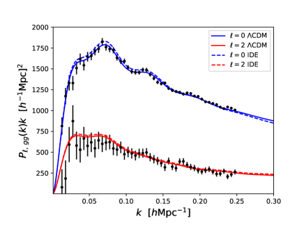
The theoretical predictions for the monopole () and quadrupole () of the full-shape power spectrum within CDM and the IDE model considered here are shown in Fig. 1. We have fixed the cosmological parameters to the best-fit values obtained from a combined analysis of CMB, pre-reconstructed FS, and post-reconstruction BAO data (see details in Secs. III and IV), whereas we have fixed the DM-DE coupling strength to . Note that we have kept nuisance parameters fixed to their CDM best-fit values when moving across the two models, in order to focus exclusively on the effects induced by the cosmological parameters. In reality, nuisance parameters shift slightly when moving from one model to another, and as a result absorb part of the differences shown in Fig. 1. However, we have explicitly checked that the shifts in all nuisance parameters remain below the level, and that the extent to which they will absorb part of the signal of interest is rather limited. Notice from Fig. 1 that the cleanest signature of IDE appears to be in the monopole. Already from these qualitative considerations we can expect that broadband information in the FS galaxy power spectrum, and in particular information related to the equality scale, will play an important role in setting constraints on IDE. Our analysis will confirm these expectations, as we will later discuss in Sec. IV.
III Datasets and methodology
In order to set constraints on the parameters of the IDE model we shall consider various combinations of the following datasets:
-
•
Measurements of CMB temperature anisotropy and polarization power spectra, as well as their cross-spectra, from the Planck 2018 legacy data release. We consider the high- Plik likelihood for TT (in the multipole range ) as well as TE and EE (in the multipole range ), in combination with the low- TT-only () likelihood based on the Commander component-separation algorithm in pixel space, as well as the low- EE-only () SimAll likelihood Aghanim et al. (2020b). We also include measurements of the CMB lensing power spectrum, as reconstructed from the temperature 4-point function Aghanim et al. (2020c). We refer to this dataset combination as CMB.
-
•
Post-reconstruction Baryon Acoustic Oscillation measurements from the BOSS DR12 Alam et al. (2017) survey. We refer to this dataset as BAO.
-
•
Measurements of the monopole and quadrupole ( and respectively) of the full-shape power spectrum of the BOSS DR12 galaxies, divided into four independent inputs: two distinct redshift bins at and , observed in the North and South galactic caps (NGC and SGC respectively). We refer to this dataset combination as FS.
-
•
A Gaussian prior on the physical baryon density parameter arising from Big Bang Nucleosynthesis (BBN) constraints on the abundance of light elements: Mossa et al. (2020). We refer to this prior as BBN.
For more details regarding window function, post-reconstruction BAO measurements extraction, BAO-FS covariance matrix, and implementation of the joint FS+BAO likelihood, we refer the reader to Refs. Ivanov et al. (2020a); Philcox et al. (2020); Chudaykin et al. (2020), which discusses these issues in depth.
Model-wise, we consider a seven-parameter IDE model, where the strength of the DM-DE interaction is allowed to vary alongside the six standard CDM parameters. We set a flat prior on in order to avoid gravitational and early-time non-adiabatic instabilities (see Sec. II.1), verifying a posteriori that our results are not affected by the choice of lower prior boundary. We set the default, wide conservative priors on the EFTofLSS nuisance parameters following Ref. Ivanov et al. (2020a). As we are including CMB measurements, we do not fix either the scalar spectral index nor the baryon-to-dark-matter density ratio , given that both these parameters are extremely well constrained by CMB data.
Theoretical predictions for the relevant observables are obtained using the Boltzmann solver CLASS-PT Chudaykin et al. (2020), which is itself an extension of the Boltzmann solver CLASS Blas et al. (2011); Lesgourgues (2011), and allows to compute the 1-loop auto- and cross-power spectra for matter fields and biased tracers both in real and redshift space, incorporating all the ingredients discussed in Sec. II.2 required for the comparison to data. Our theoretical model for the FS measurements is based on the EFTofLSS predictions at 1-loop order (corresponding to perturbative order ), and we consider FS measurements in the wavenumber range (slightly more conservative than the wavenumber range adopted in other works which have used the very same likelihood). As explained earlier, we only modify the input linear power spectrum obtained by solving the system of coupled linear Einstein-Boltzmann equations for the IDE model given in Eqs. (9–12), without altering the SPT kernels, the structure of the counter-terms and stochastic contributions, the IR resummation implementation, and so on.777Note that, besides the EFTofLSS, a number of other theoretical modeling approaches have been adopted in analysis and forecasts for galaxy clustering data. Some of these studies considered simpler phenomenological and/or theory-motivated models for the FS power spectrum and higher order correlators, whereas others considered compressed versions thereof (see e.g. Refs. Escudero et al. (2015); Cuesta et al. (2016); Giusarma et al. (2016); Grieb et al. (2017); Sanchez et al. (2017); Beutler et al. (2017a, b); Doux et al. (2018); Gualdi et al. (2018); Sprenger et al. (2019); Gil-Marín et al. (2018); Giusarma et al. (2018); Vagnozzi et al. (2018a); Loureiro et al. (2019); Gualdi et al. (2019); Tröster et al. (2020); Chen et al. (2020); Kobayashi et al. (2020); Gil-Marin et al. (2020); Gualdi et al. (2021a); Cuceu et al. (2021); Gualdi et al. (2021b); Brieden et al. (2021a, b); Chen et al. (2022); Semenaite et al. (2021); Neveux et al. (2022); Gualdi and Verde (2022); Brieden et al. (2022); Gil-Marín (2022)).
We sample the posterior distributions for the parameters of the IDE model through Monte Carlo Markov Chain (MCMC) methods, using the cosmological sampler MontePython Audren et al. (2013); Brinckmann and Lesgourgues (2019). We assess the convergence of the MCMC chains using the Gelman-Rubin parameter Gelman and Rubin (1992), requiring for the chains to be considered converged.
When considering analyses involving the BAO dataset but not the FS one (e.g. when considering the CMB+BAO dataset combination), we make use of the “standard” non-EFTofLSS likelihood which is publicly available at github.com/brinckmann/montepython_public (in particular, we use the bao_boss_dr12 likelihood and not the bao_fs_boss_dr12 one, with the latter incorporating also measurements). When instead combining the BAO and FS datasets, we make use of the joint BAO-FS likelihood which is publicly available at github.com/oliverphilcox/full_shape_likelihoods, see Ref. Philcox et al. (2020). This strategy will provide the key to isolate the advantages of using the joint BAO-FS likelihood, and in particular the inclusion of FS measurements in the context of IDE models. In fact, thanks to our choice, our analyses involving the BAO dataset but not the FS one will be as close as possible to pre-2020 analyses which preceded the public release of the joint BAO-FS EFTofLSS likelihood we are using.888Recall that state-of-the-art constraints on IDE models mostly arise from the combination of CMB and geometrical information from the reconstructed BAO peaks, see for instance Ref. Di Valentino et al. (2020b).
| Parameter | CMB+BAO | CMB+FS | CMB+BAO+FS |
|---|---|---|---|
| Parameter | FS+BAO | FS+BAO+BBN |
|---|---|---|
IV Results
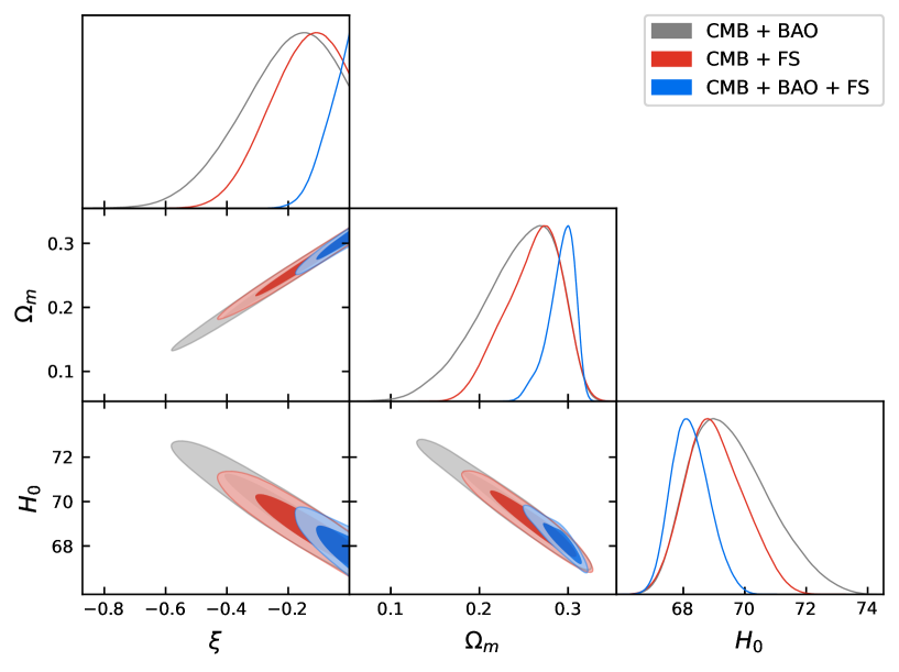
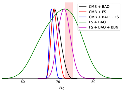
We begin by discussing the results obtained from dataset combinations involving the CMB dataset: CMB+BAO, CMB+FS, and CMB+BAO+FS. Afterwards, to better examine the role of shape versus geometrical information in setting constraints on IDE, we consider CMB-free dataset combinations: FS+BAO and FS+BAO+BBN. Our key results are reported in Tabs. 1 and 2, as well as Figs. 2, 3, and 4. Note that for we shall always report the 95% confidence level (C.L.) lower bound when the 68% C.L. interval is not consistent with a detection, whereas for all other cosmological parameters we report 68% C.L. intervals.
In the context of the CMB+BAO dataset combination, i.e the one driving state-of-the-art constraints on the DM-DE coupling strength , we infer the lower bound at 95% C.L. (while the 68% C.L. interval is ). Note that this bound is slightly weaker than those reported for instance in Refs. Di Valentino et al. (2020a, b) because we here deliberately do not include BAO measurements from the 6dFGS and SDSS-MGS surveys: however, as will become clearer later, this particular CMB+BAO dataset combination allows for a cleaner assessment of the constraining power of shape and geometrical information in the IDE context. The reason is that our pipeline does not include the 6dFGS and SDSS-MGS FS measurements. Therefore, in this setting a full comparison of the constraining power of BAO measurements from BOSS DR12+6dFGS+SDSS-MGS versus FS measurements from the same combination is not possible. We thus make the choice of restricting our LSS measurements to the one galaxy survey for which we have both a BAO and FS pipeline readily available, i.e., the BOSS DR12 galaxies. In the following, the limit obtained from the CMB+BAO dataset combination will be the reference limit to which we will compare and assess any improvement brought about by the inclusion of the FS measurements.
Including FS measurements (CMB+BAO+FS) by means of the joint BAO-FS EFTofLSS likelihood) tightens the limit on to at 95% C.L., representing a significant improvement. There is, in fact, significant information contained in the BOSS DR12 FS measurements which helps disentangling IDE from CDM. This is clear from the previous arguments in Sec. II.2, where we discussed the important role of the equality wavenumber in constraining IDE, as well as from Fig. 1.
To further examine the impact of the shape information, we now consider the CMB+FS dataset combination. The limit we obtain is at 95% C.L., tighter than that obtained from the CMB+BAO dataset combination, implying that BOSS full-shape information carries more constraining power than the purely geometrical information from the reconstructed BAO wiggles after combining with CMB data. The inferred values of selected cosmological parameters from the three dataset combinations (CMB+BAO, CMB+FS and CMB+BAO+FS) are reported in Tab. 1. In addition, the -- triangular plot in Fig. 2 clearly shows the increased constraining power of the CMB+FS dataset combination with respect to the CMB+BAO one, as well as the overall significant improvement when considering the CMB+FS+BAO dataset combination, which constitutes one of the novel results of this work.
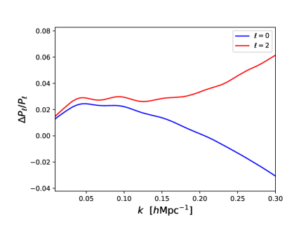
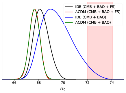
At first glance, the above results might not appear to be surprising: after all, FS information encodes geometrical BAO information in the form of wiggles in , alongside other additional information contained in the broadband, non-wiggly part of . However, this conclusion should nonetheless surprise us, as a number of recent works have argued that shape and geometrical information carry similar constraining power in light of the precision of current data Ivanov et al. (2020b). The EFTofLSS-based analysis of Ref. Ivanov et al. (2020b) argued that the comparable constraining power of shape and geometrical information in current BOSS data is purely a coincidence given the BOSS volume and redshift coverage, in combination with the efficiency of BAO reconstruction algorithms. However, Ref. Ivanov et al. (2020b) also argued that FS information is expected to dramatically supersede geometrical information in the context of future galaxy redshift surveys whose coverage will expand to significantly wider volumes and redshift ranges. Similar conclusions, albeit obtained from simpler (non-EFTofLSS) analyses of FS information, have been reached in at least two earlier works Hamann et al. (2010); Vagnozzi et al. (2017). These works also discussed the possibility of such a conclusion being reversed in extensions to CDM where shape information might play a crucial role, for instance in the context of beyond- DE models. Our results indeed provide a clear example in this sense: this further highlights the extremely important role of full-shape galaxy clustering information when probing non-standard extensions of CDM, particularly in the DE sector, such as IDE models. In fact, as we have already argued earlier in Sec. II.2, information on the equality wavenumber , not present in post-reconstruction BAO measurements, plays an important role in constraining IDE. A visual indication of the gain in constraining power when including the FS dataset (in particular when moving from the CMB+BAO dataset combination to the CMB+BAO+FS one) is given in the right panel of Fig. 3, where it is clear that there is virtually no improvement within the CDM scenario (green versus red curves), while the improvement is rather significant for the IDE model (blue versus black curves).
To further understand the role of geometrical and equality information in our results, we will closely follow the rationale of Refs. Philcox et al. (2021); Farren et al. (2022), and consider additional dataset combinations not including CMB measurements. Full-shape measurements contain the imprint of two “standard rulers”: the first is connected to the scale of the sound horizon at baryon drag , and leaves its imprint in the position of the BAO wiggles, whereas the second is connected to the horizon wavenumber at matter-radiation equality , and governs the position of the turnaround in the power spectrum, see Sec. II.2. Information from both scales can be used to constrain or, for that matter, any other parameter which affects and either directly or indirectly.999An example of a parameter indirectly influencing or is one that does so through the induced shifts in other parameters. For instance, besides their direct impact on clear from Eq. (7), which obviously affects , IDE models typically lead to shifts in , which translate into additional shifts in and in the redshift of matter-radiation equality , and therefore in .
One way of assessing the extent to which constraints involving FS data are driven by geometrical BAO information is to artificially limit or even remove any information on whatsoever. To zeroth order, this can be achieved by removing any external calibration on , which is tantamount to removing any external informative prior on the physical baryon density : FS analyses not including CMB data typically include a BBN prior on (see e.g. Ref. Philcox et al. (2020)), given that knowledge of (which controls the pre-recombination baryon sound speed) is required to compute and therefore calibrate the geometrical BAO information. Notice that this procedure is not exactly equivalent to marginalizing over , which is the proper procedure to follow to remove any geometrical information and extract only information from the broadband part of FS measurements. Nevertheless, given the precision of current galaxy clustering data, this procedure works (as argued in Ref. Philcox et al. (2021)), whereas for future, more precise FS data, the BAO features and the small-scale -induced Jeans suppression in FS measurements could in principle cross-calibrate each other, effectively generating an or prior. The later work of Ref. Farren et al. (2022) constructs an improved method to remove geometrical information in galaxy clustering measurements in future surveys. For the purposes of the present work however, given the precision of BOSS FS measurements, removing any external informative prior on is sufficient to ensure that the sound horizon information is essentially completely (or mostly) removed, and we will therefore follow the methodology of Ref. Philcox et al. (2021).
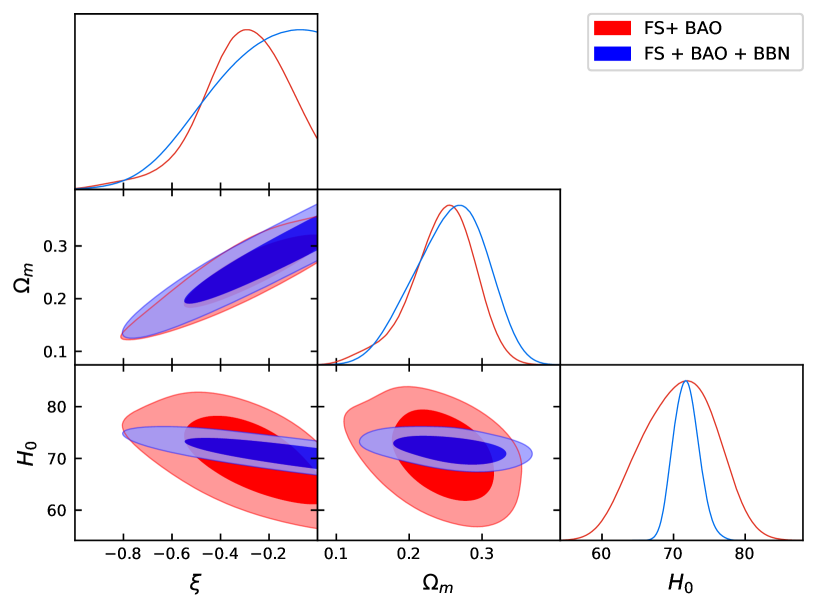
In light of the above discussion, we shall now consider the FS+BAO+BBN and FS+BAO dataset combinations: the former allows for the exploitation of sound horizon information through the BBN prior on , which calibrates , whereas such information is absent in the latter.101010Note that any dataset combination involving the CMB dataset contains information on and therefore , as is determined by the relative height of the odd versus even peaks. When considering FS+BAO+BBN we infer at 95% C.L., whereas removing the BBN prior on (thus considering the FS+BAO dataset combination) surprisingly returns exactly the same lower limit on , although in this case the 68% C.L. interval is consistent with a detection: . This further confirms the fact that the constraints on are driven to an important amount by broadband information rather than by just geometrical information: if the latter were true, the constraints on should have become significantly weaker when removing the BBN dataset, contrary to what we observe. The inferred values of selected cosmological parameters from the two CMB-free dataset combinations discussed above are reported in Tab. 2, whereas in Fig. 4 we present the -- triangular plot obtained from these same two dataset combinations.
It is important to explore the impact of the inclusion of FS measurements on the inference of parameters other than the coupling . There are two key parameters in IDE cosmologies: the matter density parameter and the Hubble constant . The correlation between and can be understood in terms of the direction of energy flow between DM and DE. Since , energy flows from DM to DE, and therefore the DM density today (and correspondingly ) will be smaller Di Valentino et al. (2020a, b). This is also clear from Eq. (7), where the evolution of carries an extra term proportional to in addition to the standard CDM term . However, as is tightly constrained by CMB data, the decrease in requires an increase in . This explains the mutual -- degeneracies we observe: a direct correlation between and , and an inverse correlation between and , with a significantly weaker inverse correlation between and . Focusing on and , we find that their determination is significantly improved by the inclusion of the FS dataset on top of the CMB+BAO dataset combination. In particular, the uncertainties on and are decreased by factors of 3 and 2 respectively. This improvement (particularly for ) is due to the important role of the equality scale in FS measurements. In fact, equality information in FS measurements directly constrains the so-called “shape parameter” Efstathiou et al. (1992, 2002). In combination with CMB measurements constraining through the early integrated Sachs-Wolfe Hou et al. (2013); Cabass et al. (2015); Kable et al. (2020); Vagnozzi (2021) and lensing effects Baxter and Sherwin (2021), and geometrical BAO information, this helps pinning down , particularly in the context of extended models (see for instance the discussion in Section 2 of Ref. Vagnozzi et al. (2021b) in the context of spatial curvature). In Sec. II.2 we already emphasized the important role of broadband information (and in particular information related to ) in the context of IDE models, which is anyhow clear from the monopole curves in Fig. 1.
Moving to the CMB-free dataset combinations discussed earlier (FS+BAO and FS+BAO+BBN), we note that the parameter most significantly affected by the addition of the BBN prior on is the Hubble constant , whose uncertainty decreases by a factor of once the BBN dataset is included. This is not surprising, given that current galaxy clustering data mostly constrain through the sound horizon rather than from equality scale information Philcox et al. (2021). The uncertainty we infer on of order is in fact comparable to that obtained in Ref. Philcox et al. (2021) for the CDM model (of course, our uncertainties are slightly larger because of the extra parameter and its correlation with ). To conclude this section, it is clear that full-shape information is highly precious when dealing with non-trivial extensions of the CDM model, particularly within IDE cosmologies. The addition of FS information further limits the available parameter space for the DM-DE coupling strength, even in the absence of CMB data.
V Conclusions
Driven by important theoretical advances, in the last couple of years significant efforts have gone into extracting Large-Scale Structure (LSS) clustering information beyond geometrical information contained in the reconstructed BAO peaks, by exploiting the information content of the full-shape (FS) power spectrum of LSS tracers. The power of FS measurements and their ability to not only sharpen constraints on the parameters of the baseline CDM model, but perhaps more importantly test extensions thereof, is by now established. In the wake of these important developments, the present work is the first to test interacting dark energy (IDE) cosmologies in light of state-of-the-art redshift-space galaxy clustering data, with a robust theoretical modeling of the underlying mildly non-linear power spectrum.
IDE cosmologies feature non-gravitational interactions between dark matter (DM) and dark energy (DE) and have experienced nothing short of a resurgence in recent years. In the context of our work, IDE models provide a unique phenomenological stage to test the power and advantages of certain cosmological observations with respect to others. Specifically, our goal is to assess the improvement gained by considering FS measurements when constraining the DM-DE coupling strength , taking as baseline state-of-the-art constraints which only consider geometrical BAO measurements (see e.g. Ref. Di Valentino et al. (2020b)). Focusing on an IDE model [see Eq. (4)] which is well-studied, mostly due to its simplicity and connection to coupled quintessence, we have demonstrated how the inclusion of FS measurements significantly sharpens constraints on , which is now safely constrained to for the model considered.
Our limits on imply that DM and DE cannot exchange energy at a rate greater than , or equivalently that they cannot exchange more than of the critical energy density over the course of a Hubble time, a quantity which is way too small to have any bearings on the coincidence problem (as was already known). Moreover, these tight constraints further limit the ability of IDE cosmologies to play an important role in the context of the Hubble tension. Crucially, the same limits also constrain the DE effective equation of state (EoS) , consistent with independent constraints on the DE EoS from various probes, which strongly limit the ability to move deep into the phantom region (see e.g. Refs. Zhao et al. (2017); Vagnozzi et al. (2018b); Gerardi et al. (2019); Vagnozzi (2020); Visinelli et al. (2019); Bonilla et al. (2021); Colgáin et al. (2021); Teng et al. (2021); Raveri et al. (2021); Sharma et al. (2022)). 111111Our results, and particularly the inferred values of , can also be compared to those of Ref. Krishnan et al. (2021), given the background equivalence between IDE and dynamical DE models.
Our results highlight the extremely important role of FS measurements in the era of precision cosmology, particularly in further sharpening constraints on models beyond CDM: for instance, a recently well-documented example in this context is that of the early dark energy model Hill et al. (2020); Ivanov et al. (2020c); D’Amico et al. (2021b); Niedermann and Sloth (2020); Smith et al. (2021); Ye et al. (2021b); Poulin et al. (2021); La Posta et al. (2021); Smith et al. (2022); Jiang and Piao (2022). 121212See also Ref. Rudelius (2022) for related discussions on theoretical difficulties early dark energy faces. Furthermore, contrary to what occurs within the CDM model and simple extensions thereof, we have demonstrated that constraints obtained by combining CMB and FS data are tighter than those obtained by combining CMB and BAO measurements, suggesting that in the context of IDE models there is significant information contained in the broadband of the power spectrum. We have extensively tested these findings, discussing the important role played by the equality scale in constraining IDE cosmologies.
This work is the first to robustly test DM-DE interactions from state-of-the-art redshift-space galaxy clustering measurements, and the constraints we report on the coupling strength are among the strongest ever presented in the literature. At the same time, there are many interesting follow-up directions one could envisage. While here we have considered FS measurements from the BOSS DR12 sample, it would be very interesting to repeat a similar analysis using the much more recent eBOSS DR16 measurements Alam et al. (2021). On the other hand, we expect the role of FS galaxy clustering information to become even more important in this context with the advent of future LSS surveys, such as Euclid Amendola et al. (2018) and DESI Aghamousa et al. (2016). It would be interesting to forecast the ability of these surveys to constrain DM-DE interactions when combined with future CMB data, for instance from Simons Observatory Ade et al. (2019); Abitbol et al. (2019) or CMB-S4 Abazajian et al. (2016). Finally, it would be very interesting to test other well-motivated beyond-CDM models in light of the same FS measurements adopted here. Most of these ideas are the subject of work in progress, on which we hope to report soon.
Acknowledgements.
S.V. thanks Misha Ivanov for useful discussions. R.C.N. acknowledges financial support from the Fundação de Amparo à Pesquisa do Estado de São Paulo (FAPESP, São Paulo Research Foundation) under the project No. 2018/18036-5. S.V. is supported by the Isaac Newton Trust and the Kavli Foundation through a Newton-Kavli Fellowship, and by a grant from the Foundation Blanceflor Boncompagni Ludovisi, née Bildt. S.V. acknowledges a College Research Associateship at Homerton College, University of Cambridge. S.K. gratefully acknowledges support from the Science and Engineering Research Board (SERB), Govt. of India (File No. CRG/2021/004658). E.D.V. is supported by a Royal Society Dorothy Hodgkin Research Fellowship. O.M. is supported by the Spanish grants PID2020-113644GB-I00, PROMETEO/2019/083 and by the European ITN project HIDDeN (H2020-MSCA-ITN-2019//860881-HIDDeN).References
- Riess et al. (1998) A. G. Riess et al. (Supernova Search Team), Astron. J. 116, 1009 (1998), arXiv:astro-ph/9805201 .
- Perlmutter et al. (1999) S. Perlmutter et al. (Supernova Cosmology Project), Astrophys. J. 517, 565 (1999), arXiv:astro-ph/9812133 .
- Aghanim et al. (2020a) N. Aghanim et al. (Planck), Astron. Astrophys. 641, A6 (2020a), [Erratum: Astron.Astrophys. 652, C4 (2021)], arXiv:1807.06209 [astro-ph.CO] .
- Aiola et al. (2020) S. Aiola et al. (ACT), JCAP 12, 047 (2020), arXiv:2007.07288 [astro-ph.CO] .
- Alam et al. (2021) S. Alam et al. (eBOSS), Phys. Rev. D 103, 083533 (2021), arXiv:2007.08991 [astro-ph.CO] .
- Asgari et al. (2021) M. Asgari et al. (KiDS), Astron. Astrophys. 645, A104 (2021), arXiv:2007.15633 [astro-ph.CO] .
- Mossa et al. (2020) V. Mossa et al., Nature 587, 210 (2020).
- Dutcher et al. (2021) D. Dutcher et al. (SPT-3G), Phys. Rev. D 104, 022003 (2021), arXiv:2101.01684 [astro-ph.CO] .
- Abbott et al. (2022) T. M. C. Abbott et al. (DES), Phys. Rev. D 105, 023520 (2022), arXiv:2105.13549 [astro-ph.CO] .
- Scolnic et al. (2021) D. Scolnic et al., (2021), arXiv:2112.03863 [astro-ph.CO] .
- Weinberg (1989) S. Weinberg, Rev. Mod. Phys. 61, 1 (1989).
- Wetterich (1988) C. Wetterich, Nucl. Phys. B 302, 668 (1988), arXiv:1711.03844 [hep-th] .
- Ratra and Peebles (1988) B. Ratra and P. J. E. Peebles, Phys. Rev. D 37, 3406 (1988).
- Caldwell et al. (1998) R. R. Caldwell, R. Dave, and P. J. Steinhardt, Phys. Rev. Lett. 80, 1582 (1998), arXiv:astro-ph/9708069 .
- Zlatev et al. (1999) I. Zlatev, L.-M. Wang, and P. J. Steinhardt, Phys. Rev. Lett. 82, 896 (1999), arXiv:astro-ph/9807002 .
- Huey and Wandelt (2006) G. Huey and B. D. Wandelt, Phys. Rev. D 74, 023519 (2006), arXiv:astro-ph/0407196 .
- Velten et al. (2014) H. E. S. Velten, R. F. vom Marttens, and W. Zimdahl, Eur. Phys. J. C 74, 3160 (2014), arXiv:1410.2509 [astro-ph.CO] .
- D’Amico et al. (2016) G. D’Amico, T. Hamill, and N. Kaloper, Phys. Rev. D 94, 103526 (2016), arXiv:1605.00996 [hep-th] .
- Marsh (2017) M. C. D. Marsh, Phys. Rev. Lett. 118, 011302 (2017), arXiv:1606.01538 [astro-ph.CO] .
- Di Valentino et al. (2017) E. Di Valentino, A. Melchiorri, and O. Mena, Phys. Rev. D 96, 043503 (2017), arXiv:1704.08342 [astro-ph.CO] .
- Yang et al. (2019a) W. Yang, O. Mena, S. Pan, and E. Di Valentino, Phys. Rev. D 100, 083509 (2019a), arXiv:1906.11697 [astro-ph.CO] .
- Cheng et al. (2020) G. Cheng, Y.-Z. Ma, F. Wu, J. Zhang, and X. Chen, Phys. Rev. D 102, 043517 (2020), arXiv:1911.04520 [astro-ph.CO] .
- Yang et al. (2020a) W. Yang, E. Di Valentino, O. Mena, and S. Pan, Phys. Rev. D 102, 023535 (2020a), arXiv:2003.12552 [astro-ph.CO] .
- Yang et al. (2021a) W. Yang, S. Pan, L. Aresté Saló, and J. de Haro, Phys. Rev. D 103, 083520 (2021a), arXiv:2104.04505 [astro-ph.CO] .
- Zhang et al. (2019) J. Zhang, R. An, W. Luo, Z. Li, S. Liao, and B. Wang, Astrophys. J. Lett. 875, L11 (2019), arXiv:1807.05522 [astro-ph.CO] .
- Zhang et al. (2018) J. Zhang, R. An, S. Liao, W. Luo, Z. Li, and B. Wang, Phys. Rev. D 98, 103530 (2018), arXiv:1811.01519 [astro-ph.CO] .
- Liu et al. (2022) Y. Liu, S. Liao, X. Liu, J. Zhang, R. An, and Z. Fan, Mon. Not. Roy. Astron. Soc. 511, 3076 (2022), arXiv:2201.09817 [astro-ph.CO] .
- Bernal et al. (2016) J. L. Bernal, L. Verde, and A. G. Riess, JCAP 10, 019 (2016), arXiv:1607.05617 [astro-ph.CO] .
- Addison et al. (2018) G. E. Addison, D. J. Watts, C. L. Bennett, M. Halpern, G. Hinshaw, and J. L. Weiland, Astrophys. J. 853, 119 (2018), arXiv:1707.06547 [astro-ph.CO] .
- Mörtsell and Dhawan (2018) E. Mörtsell and S. Dhawan, JCAP 09, 025 (2018), arXiv:1801.07260 [astro-ph.CO] .
- Lemos et al. (2019) P. Lemos, E. Lee, G. Efstathiou, and S. Gratton, Mon. Not. Roy. Astron. Soc. 483, 4803 (2019), arXiv:1806.06781 [astro-ph.CO] .
- Aylor et al. (2019) K. Aylor, M. Joy, L. Knox, M. Millea, S. Raghunathan, and W. L. K. Wu, Astrophys. J. 874, 4 (2019), arXiv:1811.00537 [astro-ph.CO] .
- Knox and Millea (2020) L. Knox and M. Millea, Phys. Rev. D 101, 043533 (2020), arXiv:1908.03663 [astro-ph.CO] .
- Arendse et al. (2020) N. Arendse et al., Astron. Astrophys. 639, A57 (2020), arXiv:1909.07986 [astro-ph.CO] .
- Zhang and Huang (2021) X. Zhang and Q.-G. Huang, Phys. Rev. D 103, 043513 (2021), arXiv:2006.16692 [astro-ph.CO] .
- Efstathiou (2021) G. Efstathiou, Mon. Not. Roy. Astron. Soc. 505, 3866 (2021), arXiv:2103.08723 [astro-ph.CO] .
- Cai et al. (2022) R.-G. Cai, Z.-K. Guo, S.-J. Wang, W.-W. Yu, and Y. Zhou, Phys. Rev. D 105, L021301 (2022), arXiv:2107.13286 [astro-ph.CO] .
- Di Valentino et al. (2021a) E. Di Valentino et al., Astropart. Phys. 131, 102605 (2021a), arXiv:2008.11284 [astro-ph.CO] .
- Di Valentino et al. (2021b) E. Di Valentino, O. Mena, S. Pan, L. Visinelli, W. Yang, A. Melchiorri, D. F. Mota, A. G. Riess, and J. Silk, Class. Quant. Grav. 38, 153001 (2021b), arXiv:2103.01183 [astro-ph.CO] .
- Perivolaropoulos and Skara (2021) L. Perivolaropoulos and F. Skara, (2021), arXiv:2105.05208 [astro-ph.CO] .
- Schöneberg et al. (2021) N. Schöneberg, G. Franco Abellán, A. Pérez Sánchez, S. J. Witte, V. Poulin, and J. Lesgourgues, (2021), arXiv:2107.10291 [astro-ph.CO] .
- Abdalla et al. (2022) E. Abdalla et al. (2022) arXiv:2203.06142 [astro-ph.CO] .
- Baumann et al. (2012) D. Baumann, A. Nicolis, L. Senatore, and M. Zaldarriaga, JCAP 07, 051 (2012), arXiv:1004.2488 [astro-ph.CO] .
- Gavela et al. (2009) M. B. Gavela, D. Hernandez, L. Lopez Honorez, O. Mena, and S. Rigolin, JCAP 07, 034 (2009), [Erratum: JCAP 05, E01 (2010)], arXiv:0901.1611 [astro-ph.CO] .
- Duniya et al. (2015) D. G. A. Duniya, D. Bertacca, and R. Maartens, Phys. Rev. D 91, 063530 (2015), arXiv:1502.06424 [astro-ph.CO] .
- Carroll (1998) S. M. Carroll, Phys. Rev. Lett. 81, 3067 (1998), arXiv:astro-ph/9806099 .
- Wetterich (1995) C. Wetterich, Astron. Astrophys. 301, 321 (1995), arXiv:hep-th/9408025 .
- Amendola (2000a) L. Amendola, Mon. Not. Roy. Astron. Soc. 312, 521 (2000a), arXiv:astro-ph/9906073 .
- Amendola (2000b) L. Amendola, Phys. Rev. D 62, 043511 (2000b), arXiv:astro-ph/9908023 .
- Mangano et al. (2003) G. Mangano, G. Miele, and V. Pettorino, Mod. Phys. Lett. A 18, 831 (2003), arXiv:astro-ph/0212518 .
- Farrar and Peebles (2004) G. R. Farrar and P. J. E. Peebles, Astrophys. J. 604, 1 (2004), arXiv:astro-ph/0307316 .
- Vagnozzi et al. (2020) S. Vagnozzi, L. Visinelli, O. Mena, and D. F. Mota, Mon. Not. Roy. Astron. Soc. 493, 1139 (2020), arXiv:1911.12374 [gr-qc] .
- Jiménez et al. (2020) J. B. Jiménez, D. Bettoni, D. Figueruelo, and F. A. Teppa Pannia, JCAP 08, 020 (2020), arXiv:2004.14661 [astro-ph.CO] .
- Vagnozzi et al. (2021a) S. Vagnozzi, L. Visinelli, P. Brax, A.-C. Davis, and J. Sakstein, Phys. Rev. D 104, 063023 (2021a), arXiv:2103.15834 [hep-ph] .
- Benisty and Davis (2022) D. Benisty and A.-C. Davis, Phys. Rev. D 105, 024052 (2022), arXiv:2108.06286 [astro-ph.CO] .
- Ferlito et al. (2022) F. Ferlito, S. Vagnozzi, D. F. Mota, and M. Baldi, (2022), arXiv:2201.04528 [astro-ph.CO] .
- Calabrese et al. (2014) E. Calabrese, M. Martinelli, S. Pandolfi, V. F. Cardone, C. J. A. P. Martins, S. Spiro, and P. E. Vielzeuf, Phys. Rev. D 89, 083509 (2014), arXiv:1311.5841 [astro-ph.CO] .
- Martins and Pinho (2015) C. J. A. P. Martins and A. M. M. Pinho, Phys. Rev. D 91, 103501 (2015), arXiv:1505.02196 [astro-ph.CO] .
- Martins et al. (2015) C. J. A. P. Martins, A. M. M. Pinho, R. F. C. Alves, M. Pino, C. I. S. A. Rocha, and M. von Wietersheim, JCAP 08, 047 (2015), arXiv:1508.06157 [astro-ph.CO] .
- Martins et al. (2016) C. J. A. P. Martins, A. M. M. Pinho, P. Carreira, A. Gusart, J. López, and C. I. S. A. Rocha, Phys. Rev. D 93, 023506 (2016), arXiv:1601.02950 [astro-ph.CO] .
- Martinelli et al. (2021) M. Martinelli et al. (Euclid), Astron. Astrophys. 654, A148 (2021), arXiv:2105.09746 [astro-ph.CO] .
- He and Zhang (2017) H.-J. He and Z. Zhang, JCAP 08, 036 (2017), arXiv:1701.03418 [astro-ph.CO] .
- Zhang (2022) Z. Zhang, Class. Quant. Grav. 39, 015003 (2022), arXiv:2112.04149 [gr-qc] .
- Valiviita et al. (2008) J. Valiviita, E. Majerotto, and R. Maartens, JCAP 07, 020 (2008), arXiv:0804.0232 [astro-ph] .
- Pan et al. (2020) S. Pan, G. S. Sharov, and W. Yang, Phys. Rev. D 101, 103533 (2020), arXiv:2001.03120 [astro-ph.CO] .
- Gavela et al. (2010) M. B. Gavela, L. Lopez Honorez, O. Mena, and S. Rigolin, JCAP 11, 044 (2010), arXiv:1005.0295 [astro-ph.CO] .
- Lopez Honorez et al. (2010) L. Lopez Honorez, B. A. Reid, O. Mena, L. Verde, and R. Jimenez, JCAP 09, 029 (2010), arXiv:1006.0877 [astro-ph.CO] .
- Di Valentino and Mena (2020) E. Di Valentino and O. Mena, Mon. Not. Roy. Astron. Soc. 500, L22 (2020), arXiv:2009.12620 [astro-ph.CO] .
- Banerjee et al. (2021) A. Banerjee, H. Cai, L. Heisenberg, E. O. Colgáin, M. M. Sheikh-Jabbari, and T. Yang, Phys. Rev. D 103, L081305 (2021), arXiv:2006.00244 [astro-ph.CO] .
- Di Valentino et al. (2020a) E. Di Valentino, A. Melchiorri, O. Mena, and S. Vagnozzi, Phys. Dark Univ. 30, 100666 (2020a), arXiv:1908.04281 [astro-ph.CO] .
- Di Valentino et al. (2020b) E. Di Valentino, A. Melchiorri, O. Mena, and S. Vagnozzi, Phys. Rev. D 101, 063502 (2020b), arXiv:1910.09853 [astro-ph.CO] .
- Lucca and Hooper (2020) M. Lucca and D. C. Hooper, Phys. Rev. D 102, 123502 (2020), arXiv:2002.06127 [astro-ph.CO] .
- Li et al. (2014a) Y.-H. Li, J.-F. Zhang, and X. Zhang, Phys. Rev. D 90, 063005 (2014a), arXiv:1404.5220 [astro-ph.CO] .
- Li et al. (2014b) Y.-H. Li, J.-F. Zhang, and X. Zhang, Phys. Rev. D 90, 123007 (2014b), arXiv:1409.7205 [astro-ph.CO] .
- Guo et al. (2017) R.-Y. Guo, Y.-H. Li, J.-F. Zhang, and X. Zhang, JCAP 05, 040 (2017), arXiv:1702.04189 [astro-ph.CO] .
- Zhang (2017) X. Zhang, Sci. China Phys. Mech. Astron. 60, 050431 (2017), arXiv:1702.04564 [astro-ph.CO] .
- Guo et al. (2018a) R.-Y. Guo, J.-F. Zhang, and X. Zhang, Chin. Phys. C 42, 095103 (2018a), arXiv:1803.06910 [astro-ph.CO] .
- Amendola and Quercellini (2003) L. Amendola and C. Quercellini, Phys. Rev. D 68, 023514 (2003), arXiv:astro-ph/0303228 .
- Pettorino et al. (2005a) V. Pettorino, C. Baccigalupi, and G. Mangano, JCAP 01, 014 (2005a), arXiv:astro-ph/0412334 .
- Pettorino et al. (2005b) V. Pettorino, C. Baccigalupi, and F. Perrotta, JCAP 12, 003 (2005b), arXiv:astro-ph/0508586 .
- Barrow and Clifton (2006) J. D. Barrow and T. Clifton, Phys. Rev. D 73, 103520 (2006), arXiv:gr-qc/0604063 .
- Bean et al. (2008) R. Bean, E. E. Flanagan, and M. Trodden, Phys. Rev. D 78, 023009 (2008), arXiv:0709.1128 [astro-ph] .
- He and Wang (2008) J.-H. He and B. Wang, JCAP 06, 010 (2008), arXiv:0801.4233 [astro-ph] .
- Pettorino and Baccigalupi (2008) V. Pettorino and C. Baccigalupi, Phys. Rev. D 77, 103003 (2008), arXiv:0802.1086 [astro-ph] .
- Baldi et al. (2010) M. Baldi, V. Pettorino, G. Robbers, and V. Springel, Mon. Not. Roy. Astron. Soc. 403, 1684 (2010), arXiv:0812.3901 [astro-ph] .
- Majerotto et al. (2010) E. Majerotto, J. Valiviita, and R. Maartens, Mon. Not. Roy. Astron. Soc. 402, 2344 (2010), arXiv:0907.4981 [astro-ph.CO] .
- Jamil et al. (2010) M. Jamil, E. N. Saridakis, and M. R. Setare, Phys. Rev. D 81, 023007 (2010), arXiv:0910.0822 [hep-th] .
- Martinelli et al. (2010) M. Martinelli, L. Lopez Honorez, A. Melchiorri, and O. Mena, Phys. Rev. D 81, 103534 (2010), arXiv:1004.2410 [astro-ph.CO] .
- Baldi and Pettorino (2011) M. Baldi and V. Pettorino, Mon. Not. Roy. Astron. Soc. 412, L1 (2011), arXiv:1006.3761 [astro-ph.CO] .
- De Bernardis et al. (2011) F. De Bernardis, M. Martinelli, A. Melchiorri, O. Mena, and A. Cooray, Phys. Rev. D 84, 023504 (2011), arXiv:1104.0652 [astro-ph.CO] .
- Baldi (2012) M. Baldi, Mon. Not. Roy. Astron. Soc. 420, 430 (2012), arXiv:1107.5049 [astro-ph.CO] .
- Pettorino et al. (2012) V. Pettorino, L. Amendola, C. Baccigalupi, and C. Quercellini, Phys. Rev. D 86, 103507 (2012), arXiv:1207.3293 [astro-ph.CO] .
- Carbone et al. (2013) C. Carbone, M. Baldi, V. Pettorino, and C. Baccigalupi, JCAP 09, 004 (2013), arXiv:1305.0829 [astro-ph.CO] .
- Piloyan et al. (2013) A. Piloyan, V. Marra, M. Baldi, and L. Amendola, JCAP 07, 042 (2013), arXiv:1305.3106 [astro-ph.CO] .
- Pettorino (2013) V. Pettorino, Phys. Rev. D 88, 063519 (2013), arXiv:1305.7457 [astro-ph.CO] .
- Pourtsidou et al. (2013) A. Pourtsidou, C. Skordis, and E. J. Copeland, Phys. Rev. D 88, 083505 (2013), arXiv:1307.0458 [astro-ph.CO] .
- Piloyan et al. (2014) A. Piloyan, V. Marra, M. Baldi, and L. Amendola, JCAP 02, 045 (2014), arXiv:1401.2656 [astro-ph.CO] .
- Faraoni et al. (2014) V. Faraoni, J. B. Dent, and E. N. Saridakis, Phys. Rev. D 90, 063510 (2014), arXiv:1405.7288 [gr-qc] .
- Ferreira et al. (2017) E. G. M. Ferreira, J. Quintin, A. A. Costa, E. Abdalla, and B. Wang, Phys. Rev. D 95, 043520 (2017), arXiv:1412.2777 [astro-ph.CO] .
- Ade et al. (2016) P. A. R. Ade et al. (Planck), Astron. Astrophys. 594, A14 (2016), arXiv:1502.01590 [astro-ph.CO] .
- Skordis et al. (2015) C. Skordis, A. Pourtsidou, and E. J. Copeland, Phys. Rev. D 91, 083537 (2015), arXiv:1502.07297 [astro-ph.CO] .
- Tamanini (2015) N. Tamanini, Phys. Rev. D 92, 043524 (2015), arXiv:1504.07397 [gr-qc] .
- Marra (2016) V. Marra, Phys. Dark Univ. 13, 25 (2016), arXiv:1506.05523 [astro-ph.CO] .
- Murgia et al. (2016) R. Murgia, S. Gariazzo, and N. Fornengo, JCAP 04, 014 (2016), arXiv:1602.01765 [astro-ph.CO] .
- Pourtsidou and Tram (2016) A. Pourtsidou and T. Tram, Phys. Rev. D 94, 043518 (2016), arXiv:1604.04222 [astro-ph.CO] .
- Nunes et al. (2016) R. C. Nunes, S. Pan, and E. N. Saridakis, Phys. Rev. D 94, 023508 (2016), arXiv:1605.01712 [astro-ph.CO] .
- Kumar and Nunes (2016) S. Kumar and R. C. Nunes, Phys. Rev. D 94, 123511 (2016), arXiv:1608.02454 [astro-ph.CO] .
- Kumar and Nunes (2017a) S. Kumar and R. C. Nunes, Phys. Rev. D 96, 103511 (2017a), arXiv:1702.02143 [astro-ph.CO] .
- Benisty and Guendelman (2017) D. Benisty and E. I. Guendelman, Eur. Phys. J. C 77, 396 (2017), arXiv:1701.08667 [gr-qc] .
- Yang et al. (2018a) W. Yang, S. Pan, and J. D. Barrow, Phys. Rev. D 97, 043529 (2018a), arXiv:1706.04953 [astro-ph.CO] .
- Mifsud and Van De Bruck (2017) J. Mifsud and C. Van De Bruck, JCAP 11, 001 (2017), arXiv:1707.07667 [astro-ph.CO] .
- Yang et al. (2017) W. Yang, S. Pan, and D. F. Mota, Phys. Rev. D 96, 123508 (2017), arXiv:1709.00006 [astro-ph.CO] .
- Kumar and Nunes (2017b) S. Kumar and R. C. Nunes, Eur. Phys. J. C 77, 734 (2017b), arXiv:1709.02384 [astro-ph.CO] .
- Guo et al. (2018b) J.-J. Guo, J.-F. Zhang, Y.-H. Li, D.-Z. He, and X. Zhang, Sci. China Phys. Mech. Astron. 61, 030011 (2018b), arXiv:1710.03068 [astro-ph.CO] .
- Dutta et al. (2018) J. Dutta, W. Khyllep, E. N. Saridakis, N. Tamanini, and S. Vagnozzi, JCAP 02, 041 (2018), arXiv:1711.07290 [gr-qc] .
- Feng et al. (2019) L. Feng, J.-F. Zhang, and X. Zhang, Phys. Dark Univ. 23, 100261 (2019), arXiv:1712.03148 [astro-ph.CO] .
- Benisty and Guendelman (2018) D. Benisty and E. I. Guendelman, Phys. Rev. D 98, 023506 (2018), arXiv:1802.07981 [gr-qc] .
- Barros et al. (2019) B. J. Barros, L. Amendola, T. Barreiro, and N. J. Nunes, JCAP 01, 007 (2019), arXiv:1802.09216 [astro-ph.CO] .
- Costa et al. (2018) A. A. Costa, R. C. G. Landim, B. Wang, and E. Abdalla, Eur. Phys. J. C 78, 746 (2018), arXiv:1803.06944 [astro-ph.CO] .
- Yang et al. (2018b) W. Yang, S. Pan, E. Di Valentino, R. C. Nunes, S. Vagnozzi, and D. F. Mota, JCAP 09, 019 (2018b), arXiv:1805.08252 [astro-ph.CO] .
- von Marttens et al. (2019a) R. von Marttens, L. Casarini, D. F. Mota, and W. Zimdahl, Phys. Dark Univ. 23, 100248 (2019a), arXiv:1807.11380 [astro-ph.CO] .
- Elizalde et al. (2018) E. Elizalde, M. Khurshudyan, and S. Nojiri, Int. J. Mod. Phys. D 28, 1950019 (2018), arXiv:1809.01961 [gr-qc] .
- Guo et al. (2019) R.-Y. Guo, J.-F. Zhang, and X. Zhang, JCAP 02, 054 (2019), arXiv:1809.02340 [astro-ph.CO] .
- Yang et al. (2018c) W. Yang, A. Mukherjee, E. Di Valentino, and S. Pan, Phys. Rev. D 98, 123527 (2018c), arXiv:1809.06883 [astro-ph.CO] .
- Li et al. (2019) H.-L. Li, L. Feng, J.-F. Zhang, and X. Zhang, Sci. China Phys. Mech. Astron. 62, 120411 (2019), arXiv:1812.00319 [astro-ph.CO] .
- von Marttens et al. (2019b) R. von Marttens, V. Marra, L. Casarini, J. E. Gonzalez, and J. Alcaniz, Phys. Rev. D 99, 043521 (2019b), arXiv:1812.02333 [astro-ph.CO] .
- Cárdenas et al. (2019) V. H. Cárdenas, D. Grandón, and S. Lepe, Eur. Phys. J. C 79, 357 (2019), arXiv:1812.03540 [astro-ph.CO] .
- Benisty et al. (2019) D. Benisty, E. Guendelman, and Z. Haba, Phys. Rev. D 99, 123521 (2019), [Erratum: Phys.Rev.D 101, 049901 (2020)], arXiv:1812.06151 [gr-qc] .
- Bonici and Maggiore (2019) M. Bonici and N. Maggiore, Eur. Phys. J. C 79, 672 (2019), arXiv:1812.11176 [gr-qc] .
- Martinelli et al. (2019) M. Martinelli, N. B. Hogg, S. Peirone, M. Bruni, and D. Wands, Mon. Not. Roy. Astron. Soc. 488, 3423 (2019), arXiv:1902.10694 [astro-ph.CO] .
- Kumar et al. (2019) S. Kumar, R. C. Nunes, and S. K. Yadav, Eur. Phys. J. C 79, 576 (2019), arXiv:1903.04865 [astro-ph.CO] .
- Pan et al. (2019a) S. Pan, W. Yang, C. Singha, and E. N. Saridakis, Phys. Rev. D 100, 083539 (2019a), arXiv:1903.10969 [astro-ph.CO] .
- Li et al. (2020) C. Li, X. Ren, M. Khurshudyan, and Y.-F. Cai, Phys. Lett. B 801, 135141 (2020), arXiv:1904.02458 [astro-ph.CO] .
- Yang et al. (2019b) W. Yang, S. Vagnozzi, E. Di Valentino, R. C. Nunes, S. Pan, and D. F. Mota, JCAP 07, 037 (2019b), arXiv:1905.08286 [astro-ph.CO] .
- Pan et al. (2019b) S. Pan, W. Yang, E. Di Valentino, E. N. Saridakis, and S. Chakraborty, Phys. Rev. D 100, 103520 (2019b), arXiv:1907.07540 [astro-ph.CO] .
- Landim (2019) R. G. Landim, Eur. Phys. J. C 79, 889 (2019), arXiv:1908.03657 [gr-qc] .
- Benetti et al. (2019) M. Benetti, W. Miranda, H. A. Borges, C. Pigozzo, S. Carneiro, and J. S. Alcaniz, JCAP 12, 023 (2019), arXiv:1908.07213 [astro-ph.CO] .
- von Marttens et al. (2020) R. von Marttens, H. A. Borges, S. Carneiro, J. S. Alcaniz, and W. Zimdahl, Eur. Phys. J. C 80, 1110 (2020), arXiv:1909.10336 [gr-qc] .
- Kase and Tsujikawa (2020) R. Kase and S. Tsujikawa, Phys. Rev. D 101, 063511 (2020), arXiv:1910.02699 [gr-qc] .
- Liu et al. (2020) X.-W. Liu, C. Heneka, and L. Amendola, JCAP 05, 038 (2020), arXiv:1910.02763 [astro-ph.CO] .
- Yang et al. (2020b) W. Yang, S. Pan, R. C. Nunes, and D. F. Mota, JCAP 04, 008 (2020b), arXiv:1910.08821 [astro-ph.CO] .
- Chamings et al. (2020) F. N. Chamings, A. Avgoustidis, E. J. Copeland, A. M. Green, and A. Pourtsidou, Phys. Rev. D 101, 043531 (2020), arXiv:1912.09858 [astro-ph.CO] .
- Sharma and Dubey (2022) U. K. Sharma and V. C. Dubey, Int. J. Geom. Meth. Mod. Phys. 19, 2250010 (2022), arXiv:2001.02368 [gr-qc] .
- Yang et al. (2020c) W. Yang, E. Di Valentino, O. Mena, S. Pan, and R. C. Nunes, Phys. Rev. D 101, 083509 (2020c), arXiv:2001.10852 [astro-ph.CO] .
- Hogg et al. (2020) N. B. Hogg, M. Bruni, R. Crittenden, M. Martinelli, and S. Peirone, Phys. Dark Univ. 29, 100583 (2020), arXiv:2002.10449 [astro-ph.CO] .
- Amendola and Tsujikawa (2020) L. Amendola and S. Tsujikawa, JCAP 06, 020 (2020), arXiv:2003.02686 [gr-qc] .
- Benisty et al. (2020) D. Benisty, E. I. Guendemlan, E. Nissimov, and S. Pacheva, Int. J. Mod. Phys. D 26, 2050104 (2020), arXiv:2003.13146 [astro-ph.CO] .
- Gómez-Valent et al. (2020) A. Gómez-Valent, V. Pettorino, and L. Amendola, Phys. Rev. D 101, 123513 (2020), arXiv:2004.00610 [astro-ph.CO] .
- Aljaf et al. (2021) M. Aljaf, D. Gregoris, and M. Khurshudyan, Eur. Phys. J. C 81, 544 (2021), arXiv:2005.01891 [astro-ph.CO] .
- Di Valentino et al. (2020c) E. Di Valentino, S. Gariazzo, O. Mena, and S. Vagnozzi, JCAP 07, 045 (2020c), arXiv:2005.02062 [astro-ph.CO] .
- Mukhopadhyay et al. (2021) U. Mukhopadhyay, D. Majumdar, and K. K. Datta, Phys. Rev. D 103, 063510 (2021), arXiv:2008.09972 [astro-ph.CO] .
- Di Valentino (2021) E. Di Valentino, Mon. Not. Roy. Astron. Soc. 502, 2065 (2021), arXiv:2011.00246 [astro-ph.CO] .
- Di Valentino et al. (2021c) E. Di Valentino, A. Melchiorri, O. Mena, S. Pan, and W. Yang, Mon. Not. Roy. Astron. Soc. 502, L23 (2021c), arXiv:2011.00283 [astro-ph.CO] .
- Yao and Meng (2021) Y. Yao and X.-H. Meng, Phys. Dark Univ. 33, 100852 (2021), arXiv:2011.09160 [astro-ph.CO] .
- Beltrán Jiménez et al. (2021) J. Beltrán Jiménez, D. Bettoni, D. Figueruelo, F. A. Teppa Pannia, and S. Tsujikawa, JCAP 03, 085 (2021), arXiv:2012.12204 [astro-ph.CO] .
- Yang et al. (2021b) W. Yang, S. Pan, E. Di Valentino, O. Mena, and A. Melchiorri, JCAP 10, 008 (2021b), arXiv:2101.03129 [astro-ph.CO] .
- Sinha (2021) S. Sinha, Phys. Rev. D 103, 123547 (2021), arXiv:2101.08959 [astro-ph.CO] .
- Gao et al. (2021) L.-Y. Gao, Z.-W. Zhao, S.-S. Xue, and X. Zhang, JCAP 07, 005 (2021), arXiv:2101.10714 [astro-ph.CO] .
- Zhang et al. (2021) M. Zhang, B. Wang, P.-J. Wu, J.-Z. Qi, Y. Xu, J.-F. Zhang, and X. Zhang, Astrophys. J. 918, 56 (2021), arXiv:2102.03979 [astro-ph.CO] .
- Salzano et al. (2021) V. Salzano et al., JCAP 09, 033 (2021), arXiv:2102.06417 [astro-ph.CO] .
- Wang et al. (2021) L.-F. Wang, J.-H. Zhang, D.-Z. He, J.-F. Zhang, and X. Zhang, (2021), arXiv:2102.09331 [astro-ph.CO] .
- Benetti et al. (2021) M. Benetti, H. Borges, C. Pigozzo, S. Carneiro, and J. Alcaniz, JCAP 08, 014 (2021), arXiv:2102.10123 [astro-ph.CO] .
- Kumar (2021) S. Kumar, Phys. Dark Univ. 33, 100862 (2021), arXiv:2102.12902 [astro-ph.CO] .
- Figueruelo et al. (2021) D. Figueruelo et al., JCAP 07, 022 (2021), arXiv:2103.01571 [astro-ph.CO] .
- Bora et al. (2021) K. Bora, R. F. L. Holanda, and S. Desai, Eur. Phys. J. C 81, 596 (2021), arXiv:2105.02168 [astro-ph.CO] .
- Jiménez et al. (2021) J. B. Jiménez, D. Bettoni, D. Figueruelo, F. A. Teppa Pannia, and S. Tsujikawa, Phys. Rev. D 104, 103503 (2021), arXiv:2106.11222 [astro-ph.CO] .
- Carrilho et al. (2021a) P. Carrilho, C. Moretti, B. Bose, K. Markovič, and A. Pourtsidou, JCAP 10, 004 (2021a), arXiv:2106.13163 [astro-ph.CO] .
- Lucca (2021a) M. Lucca, Phys. Rev. D 104, 083510 (2021a), arXiv:2106.15196 [astro-ph.CO] .
- Bora et al. (2022) K. Bora, R. F. L. Holanda, S. Desai, and S. H. Pereira, Eur. Phys. J. C 82, 17 (2022), arXiv:2106.15805 [astro-ph.CO] .
- Linton et al. (2021) M. S. Linton, R. Crittenden, and A. Pourtsidou, (2021), arXiv:2107.03235 [astro-ph.CO] .
- Nunes and Di Valentino (2021) R. C. Nunes and E. Di Valentino, Phys. Rev. D 104, 063529 (2021), arXiv:2107.09151 [astro-ph.CO] .
- Anchordoqui et al. (2021) L. A. Anchordoqui, E. Di Valentino, S. Pan, and W. Yang, JHEAp 32, 121 (2021), arXiv:2107.13932 [astro-ph.CO] .
- Hogg and Bruni (2022) N. B. Hogg and M. Bruni, Mon. Not. Roy. Astron. Soc. 511, 4430 (2022), arXiv:2109.08676 [astro-ph.CO] .
- Guo et al. (2021) R.-Y. Guo, L. Feng, T.-Y. Yao, and X.-Y. Chen, JCAP 12, 036 (2021), arXiv:2110.02536 [gr-qc] .
- Alestas et al. (2021) G. Alestas, D. Camarena, E. Di Valentino, L. Kazantzidis, V. Marra, S. Nesseris, and L. Perivolaropoulos, (2021), arXiv:2110.04336 [astro-ph.CO] .
- Mancini and Pourtsidou (2022) A. S. Mancini and A. Pourtsidou, Mon. Not. Roy. Astron. Soc. 512, L44 (2022), arXiv:2110.07587 [astro-ph.CO] .
- Gariazzo et al. (2021) S. Gariazzo, E. Di Valentino, O. Mena, and R. C. Nunes, (2021), arXiv:2111.03152 [astro-ph.CO] .
- Carrilho et al. (2021b) P. Carrilho, K. Carrion, B. Bose, A. Pourtsidou, J. C. Hidalgo, L. Lombriser, and M. Baldi, (2021b), arXiv:2111.13598 [astro-ph.CO] .
- Sharma and Sur (2021) M. K. Sharma and S. Sur, (2021), arXiv:2112.08477 [astro-ph.CO] .
- Duniya (2022) D. Duniya, (2022), arXiv:2203.12582 [astro-ph.CO] .
- Wang et al. (2016) B. Wang, E. Abdalla, F. Atrio-Barandela, and D. Pavon, Rept. Prog. Phys. 79, 096901 (2016), arXiv:1603.08299 [astro-ph.CO] .
- Eisenstein et al. (2007) D. J. Eisenstein, H.-j. Seo, E. Sirko, and D. Spergel, Astrophys. J. 664, 675 (2007), arXiv:astro-ph/0604362 .
- Sherwin and Zaldarriaga (2012) B. D. Sherwin and M. Zaldarriaga, Phys. Rev. D 85, 103523 (2012), arXiv:1202.3998 [astro-ph.CO] .
- Bose et al. (2018a) B. Bose, M. Baldi, and A. Pourtsidou, JCAP 04, 032 (2018a), arXiv:1711.10976 [astro-ph.CO] .
- Fonseca de la Bella et al. (2020) L. Fonseca de la Bella, D. Regan, D. Seery, and D. Parkinson, JCAP 07, 011 (2020), arXiv:1805.12394 [astro-ph.CO] .
- Osato et al. (2019) K. Osato, T. Nishimichi, F. Bernardeau, and A. Taruya, Phys. Rev. D 99, 063530 (2019), arXiv:1810.10104 [astro-ph.CO] .
- Bose et al. (2020) B. Bose, A. Pourtsidou, K. Markovič, and F. Beutler, Mon. Not. Roy. Astron. Soc. 493, 5301 (2020), arXiv:1905.05122 [astro-ph.CO] .
- Bose et al. (2019) B. Bose, K. Koyama, and H. A. Winther, JCAP 10, 021 (2019), arXiv:1905.05135 [astro-ph.CO] .
- Cabass et al. (2022a) G. Cabass, M. M. Ivanov, M. Lewandowski, M. Mirbabayi, and M. Simonović (2022) arXiv:2203.08232 [astro-ph.CO] .
- Scoccimarro and Frieman (1996) R. Scoccimarro and J. Frieman, Astrophys. J. Suppl. 105, 37 (1996), arXiv:astro-ph/9509047 .
- Zeldovich (1970) Y. B. Zeldovich, Astron. Astrophys. 5, 84 (1970).
- Crocce and Scoccimarro (2006) M. Crocce and R. Scoccimarro, Phys. Rev. D 73, 063519 (2006), arXiv:astro-ph/0509418 .
- Bernardeau et al. (2008) F. Bernardeau, M. Crocce, and R. Scoccimarro, Phys. Rev. D 78, 103521 (2008), arXiv:0806.2334 [astro-ph] .
- Matsubara (2008) T. Matsubara, Phys. Rev. D 78, 083519 (2008), [Erratum: Phys.Rev.D 78, 109901 (2008)], arXiv:0807.1733 [astro-ph] .
- Taruya et al. (2010) A. Taruya, T. Nishimichi, and S. Saito, Phys. Rev. D 82, 063522 (2010), arXiv:1006.0699 [astro-ph.CO] .
- Bernardeau et al. (2012) F. Bernardeau, M. Crocce, and R. Scoccimarro, Phys. Rev. D 85, 123519 (2012), arXiv:1112.3895 [astro-ph.CO] .
- Carlson et al. (2013) J. Carlson, B. Reid, and M. White, Mon. Not. Roy. Astron. Soc. 429, 1674 (2013), arXiv:1209.0780 [astro-ph.CO] .
- Vlah et al. (2016) Z. Vlah, E. Castorina, and M. White, JCAP 12, 007 (2016), arXiv:1609.02908 [astro-ph.CO] .
- Hand et al. (2017) N. Hand, U. Seljak, F. Beutler, and Z. Vlah, JCAP 10, 009 (2017), arXiv:1706.02362 [astro-ph.CO] .
- Chen et al. (2021) S.-F. Chen, Z. Vlah, E. Castorina, and M. White, JCAP 03, 100 (2021), arXiv:2012.04636 [astro-ph.CO] .
- McDonald and Roy (2009) P. McDonald and A. Roy, JCAP 08, 020 (2009), arXiv:0902.0991 [astro-ph.CO] .
- Carrasco et al. (2012) J. J. M. Carrasco, M. P. Hertzberg, and L. Senatore, JHEP 09, 082 (2012), arXiv:1206.2926 [astro-ph.CO] .
- Pajer and Zaldarriaga (2013) E. Pajer and M. Zaldarriaga, JCAP 08, 037 (2013), arXiv:1301.7182 [astro-ph.CO] .
- Carrasco et al. (2014a) J. J. M. Carrasco, S. Foreman, D. Green, and L. Senatore, JCAP 07, 056 (2014a), arXiv:1304.4946 [astro-ph.CO] .
- Mercolli and Pajer (2014) L. Mercolli and E. Pajer, JCAP 03, 006 (2014), arXiv:1307.3220 [astro-ph.CO] .
- Carrasco et al. (2014b) J. J. M. Carrasco, S. Foreman, D. Green, and L. Senatore, JCAP 07, 057 (2014b), arXiv:1310.0464 [astro-ph.CO] .
- Carroll et al. (2014) S. M. Carroll, S. Leichenauer, and J. Pollack, Phys. Rev. D 90, 023518 (2014), arXiv:1310.2920 [hep-th] .
- Porto et al. (2014) R. A. Porto, L. Senatore, and M. Zaldarriaga, JCAP 05, 022 (2014), arXiv:1311.2168 [astro-ph.CO] .
- Senatore and Zaldarriaga (2015) L. Senatore and M. Zaldarriaga, JCAP 02, 013 (2015), arXiv:1404.5954 [astro-ph.CO] .
- Baldauf et al. (2015a) T. Baldauf, L. Mercolli, M. Mirbabayi, and E. Pajer, JCAP 05, 007 (2015a), arXiv:1406.4135 [astro-ph.CO] .
- Angulo et al. (2015a) R. E. Angulo, S. Foreman, M. Schmittfull, and L. Senatore, JCAP 10, 039 (2015a), arXiv:1406.4143 [astro-ph.CO] .
- Senatore (2015) L. Senatore, JCAP 11, 007 (2015), arXiv:1406.7843 [astro-ph.CO] .
- Senatore and Zaldarriaga (2014) L. Senatore and M. Zaldarriaga, (2014), arXiv:1409.1225 [astro-ph.CO] .
- Lewandowski et al. (2015) M. Lewandowski, A. Perko, and L. Senatore, JCAP 05, 019 (2015), arXiv:1412.5049 [astro-ph.CO] .
- Mirbabayi et al. (2015) M. Mirbabayi, F. Schmidt, and M. Zaldarriaga, JCAP 07, 030 (2015), arXiv:1412.5169 [astro-ph.CO] .
- McQuinn and White (2016) M. McQuinn and M. White, JCAP 01, 043 (2016), arXiv:1502.07389 [astro-ph.CO] .
- Foreman and Senatore (2016) S. Foreman and L. Senatore, JCAP 04, 033 (2016), arXiv:1503.01775 [astro-ph.CO] .
- Angulo et al. (2015b) R. Angulo, M. Fasiello, L. Senatore, and Z. Vlah, JCAP 09, 029 (2015b), arXiv:1503.08826 [astro-ph.CO] .
- Baldauf et al. (2015b) T. Baldauf, M. Mirbabayi, M. Simonović, and M. Zaldarriaga, Phys. Rev. D 92, 043514 (2015b), arXiv:1504.04366 [astro-ph.CO] .
- Assassi et al. (2015a) V. Assassi, D. Baumann, E. Pajer, Y. Welling, and D. van der Woude, JCAP 11, 024 (2015a), arXiv:1505.06668 [astro-ph.CO] .
- Baldauf et al. (2016a) T. Baldauf, E. Schaan, and M. Zaldarriaga, JCAP 03, 017 (2016a), arXiv:1505.07098 [astro-ph.CO] .
- Baldauf et al. (2016b) T. Baldauf, E. Schaan, and M. Zaldarriaga, JCAP 03, 007 (2016b), arXiv:1507.02255 [astro-ph.CO] .
- Baldauf et al. (2015c) T. Baldauf, L. Mercolli, and M. Zaldarriaga, Phys. Rev. D 92, 123007 (2015c), arXiv:1507.02256 [astro-ph.CO] .
- Foreman et al. (2016) S. Foreman, H. Perrier, and L. Senatore, JCAP 05, 027 (2016), arXiv:1507.05326 [astro-ph.CO] .
- Abolhasani et al. (2016) A. A. Abolhasani, M. Mirbabayi, and E. Pajer, JCAP 05, 063 (2016), arXiv:1509.07886 [hep-th] .
- Assassi et al. (2015b) V. Assassi, D. Baumann, and F. Schmidt, JCAP 12, 043 (2015b), arXiv:1510.03723 [astro-ph.CO] .
- Lewandowski et al. (2018) M. Lewandowski, L. Senatore, F. Prada, C. Zhao, and C.-H. Chuang, Phys. Rev. D 97, 063526 (2018), arXiv:1512.06831 [astro-ph.CO] .
- Bertolini et al. (2016a) D. Bertolini, K. Schutz, M. P. Solon, J. R. Walsh, and K. M. Zurek, Phys. Rev. D 93, 123505 (2016a), arXiv:1512.07630 [astro-ph.CO] .
- Bertolini et al. (2016b) D. Bertolini, K. Schutz, M. P. Solon, and K. M. Zurek, JCAP 06, 052 (2016b), arXiv:1604.01770 [astro-ph.CO] .
- Blas et al. (2016) D. Blas, M. Garny, M. M. Ivanov, and S. Sibiryakov, JCAP 07, 028 (2016), arXiv:1605.02149 [astro-ph.CO] .
- Cataneo et al. (2017) M. Cataneo, S. Foreman, and L. Senatore, JCAP 04, 026 (2017), arXiv:1606.03633 [astro-ph.CO] .
- Bertolini and Solon (2016) D. Bertolini and M. P. Solon, JCAP 11, 030 (2016), arXiv:1608.01310 [astro-ph.CO] .
- Fujita et al. (2020) T. Fujita, V. Mauerhofer, L. Senatore, Z. Vlah, and R. Angulo, JCAP 01, 009 (2020), arXiv:1609.00717 [astro-ph.CO] .
- Perko et al. (2016) A. Perko, L. Senatore, E. Jennings, and R. H. Wechsler, (2016), arXiv:1610.09321 [astro-ph.CO] .
- Lewandowski et al. (2017) M. Lewandowski, A. Maleknejad, and L. Senatore, JCAP 05, 038 (2017), arXiv:1611.07966 [astro-ph.CO] .
- Lewandowski and Senatore (2017) M. Lewandowski and L. Senatore, JCAP 08, 037 (2017), arXiv:1701.07012 [astro-ph.CO] .
- Senatore and Zaldarriaga (2017) L. Senatore and M. Zaldarriaga, (2017), arXiv:1707.04698 [astro-ph.CO] .
- Simonović et al. (2018) M. Simonović, T. Baldauf, M. Zaldarriaga, J. J. Carrasco, and J. A. Kollmeier, JCAP 04, 030 (2018), arXiv:1708.08130 [astro-ph.CO] .
- Senatore and Trevisan (2018) L. Senatore and G. Trevisan, JCAP 05, 019 (2018), arXiv:1710.02178 [astro-ph.CO] .
- Nadler et al. (2018) E. O. Nadler, A. Perko, and L. Senatore, JCAP 02, 058 (2018), arXiv:1710.10308 [astro-ph.CO] .
- Bose et al. (2018b) B. Bose, K. Koyama, M. Lewandowski, F. Vernizzi, and H. A. Winther, JCAP 04, 063 (2018b), arXiv:1802.01566 [astro-ph.CO] .
- de Belsunce and Senatore (2019) R. de Belsunce and L. Senatore, JCAP 02, 038 (2019), arXiv:1804.06849 [astro-ph.CO] .
- Lewandowski and Senatore (2020) M. Lewandowski and L. Senatore, JCAP 03, 018 (2020), arXiv:1810.11855 [astro-ph.CO] .
- Konstandin et al. (2019) T. Konstandin, R. A. Porto, and H. Rubira, JCAP 11, 027 (2019), arXiv:1906.00997 [astro-ph.CO] .
- Nishimichi et al. (2020) T. Nishimichi, G. D’Amico, M. M. Ivanov, L. Senatore, M. Simonović, M. Takada, M. Zaldarriaga, and P. Zhang, Phys. Rev. D 102, 123541 (2020), arXiv:2003.08277 [astro-ph.CO] .
- Donath and Senatore (2020) Y. Donath and L. Senatore, JCAP 10, 039 (2020), arXiv:2005.04805 [astro-ph.CO] .
- Steele and Baldauf (2021a) T. Steele and T. Baldauf, Phys. Rev. D 103, 023520 (2021a), arXiv:2009.01200 [astro-ph.CO] .
- Bragança et al. (2021) D. P. L. Bragança, M. Lewandowski, D. Sekera, L. Senatore, and R. Sgier, JCAP 10, 074 (2021), arXiv:2010.02929 [astro-ph.CO] .
- Steele and Baldauf (2021b) T. Steele and T. Baldauf, Phys. Rev. D 103, 103518 (2021b), arXiv:2101.10289 [astro-ph.CO] .
- Baldauf et al. (2021) T. Baldauf, M. Garny, P. Taule, and T. Steele, Phys. Rev. D 104, 123551 (2021), arXiv:2110.13930 [astro-ph.CO] .
- D’Amico et al. (2020a) G. D’Amico, J. Gleyzes, N. Kokron, K. Markovic, L. Senatore, P. Zhang, F. Beutler, and H. Gil-Marín, JCAP 05, 005 (2020a), arXiv:1909.05271 [astro-ph.CO] .
- Ivanov et al. (2020a) M. M. Ivanov, M. Simonović, and M. Zaldarriaga, JCAP 05, 042 (2020a), arXiv:1909.05277 [astro-ph.CO] .
- Colas et al. (2020) T. Colas, G. D’amico, L. Senatore, P. Zhang, and F. Beutler, JCAP 06, 001 (2020), arXiv:1909.07951 [astro-ph.CO] .
- Ivanov et al. (2020b) M. M. Ivanov, M. Simonović, and M. Zaldarriaga, Phys. Rev. D 101, 083504 (2020b), arXiv:1912.08208 [astro-ph.CO] .
- Philcox et al. (2020) O. H. E. Philcox, M. M. Ivanov, M. Simonović, and M. Zaldarriaga, JCAP 05, 032 (2020), arXiv:2002.04035 [astro-ph.CO] .
- D’Amico et al. (2021a) G. D’Amico, L. Senatore, and P. Zhang, JCAP 01, 006 (2021a), arXiv:2003.07956 [astro-ph.CO] .
- Chudaykin et al. (2020) A. Chudaykin, M. M. Ivanov, O. H. E. Philcox, and M. Simonović, Phys. Rev. D 102, 063533 (2020), arXiv:2004.10607 [astro-ph.CO] .
- Ivanov et al. (2020c) M. M. Ivanov, E. McDonough, J. C. Hill, M. Simonović, M. W. Toomey, S. Alexander, and M. Zaldarriaga, Phys. Rev. D 102, 103502 (2020c), arXiv:2006.11235 [astro-ph.CO] .
- D’Amico et al. (2021b) G. D’Amico, L. Senatore, P. Zhang, and H. Zheng, JCAP 05, 072 (2021b), arXiv:2006.12420 [astro-ph.CO] .
- Wadekar et al. (2020) D. Wadekar, M. M. Ivanov, and R. Scoccimarro, Phys. Rev. D 102, 123521 (2020), arXiv:2009.00622 [astro-ph.CO] .
- Chudaykin et al. (2021a) A. Chudaykin, M. M. Ivanov, and M. Simonović, Phys. Rev. D 103, 043525 (2021a), arXiv:2009.10724 [astro-ph.CO] .
- Chudaykin et al. (2021b) A. Chudaykin, K. Dolgikh, and M. M. Ivanov, Phys. Rev. D 103, 023507 (2021b), arXiv:2009.10106 [astro-ph.CO] .
- D’Amico et al. (2020b) G. D’Amico, Y. Donath, L. Senatore, and P. Zhang, (2020b), arXiv:2012.07554 [astro-ph.CO] .
- Ivanov (2021) M. M. Ivanov, Phys. Rev. D 104, 103514 (2021), arXiv:2106.12580 [astro-ph.CO] .
- Ivanov et al. (2022) M. M. Ivanov, O. H. E. Philcox, M. Simonović, M. Zaldarriaga, T. Nischimichi, and M. Takada, Phys. Rev. D 105, 043531 (2022), arXiv:2110.00006 [astro-ph.CO] .
- D’Amico et al. (2021c) G. D’Amico, L. Senatore, P. Zhang, and T. Nishimichi, (2021c), arXiv:2110.00016 [astro-ph.CO] .
- Ivanov et al. (2021) M. M. Ivanov, O. H. E. Philcox, T. Nishimichi, M. Simonović, M. Takada, and M. Zaldarriaga, (2021), arXiv:2110.10161 [astro-ph.CO] .
- Philcox and Ivanov (2022) O. H. E. Philcox and M. M. Ivanov, Phys. Rev. D 105, 043517 (2022), arXiv:2112.04515 [astro-ph.CO] .
- Cabass et al. (2022b) G. Cabass, M. M. Ivanov, O. H. E. Philcox, M. Simonović, and M. Zaldarriaga, (2022b), arXiv:2201.07238 [astro-ph.CO] .
- D’Amico et al. (2022) G. D’Amico, M. Lewandowski, L. Senatore, and P. Zhang, (2022), arXiv:2201.11518 [astro-ph.CO] .
- Cusin et al. (2018) G. Cusin, M. Lewandowski, and F. Vernizzi, JCAP 04, 005 (2018), arXiv:1712.02783 [astro-ph.CO] .
- Creminelli et al. (2014) P. Creminelli, J. Gleyzes, M. Simonović, and F. Vernizzi, JCAP 02, 051 (2014), arXiv:1311.0290 [astro-ph.CO] .
- Crisostomi et al. (2020) M. Crisostomi, M. Lewandowski, and F. Vernizzi, Phys. Rev. D 101, 123501 (2020), arXiv:1909.07366 [astro-ph.CO] .
- Lewandowski (2020) M. Lewandowski, JCAP 08, 044 (2020), arXiv:1912.12292 [astro-ph.CO] .
- Niedermann and Sloth (2021) F. Niedermann and M. S. Sloth, Phys. Rev. D 103, 103537 (2021), arXiv:2009.00006 [astro-ph.CO] .
- Chudaykin et al. (2021c) A. Chudaykin, D. Gorbunov, and N. Nedelko, Phys. Rev. D 103, 043529 (2021c), arXiv:2011.04682 [astro-ph.CO] .
- Braglia et al. (2021) M. Braglia, M. Ballardini, F. Finelli, and K. Koyama, Phys. Rev. D 103, 043528 (2021), arXiv:2011.12934 [astro-ph.CO] .
- Allali et al. (2021) I. J. Allali, M. P. Hertzberg, and F. Rompineve, Phys. Rev. D 104, L081303 (2021), arXiv:2104.12798 [astro-ph.CO] .
- Laguë et al. (2022) A. Laguë, J. R. Bond, R. Hložek, K. K. Rogers, D. J. E. Marsh, and D. Grin, JCAP 01, 049 (2022), arXiv:2104.07802 [astro-ph.CO] .
- Jiang and Piao (2021) J.-Q. Jiang and Y.-S. Piao, Phys. Rev. D 104, 103524 (2021), arXiv:2107.07128 [astro-ph.CO] .
- Ye et al. (2021a) G. Ye, J. Zhang, and Y.-S. Piao, (2021a), arXiv:2107.13391 [astro-ph.CO] .
- Xu et al. (2021) W. L. Xu, J. B. Muñoz, and C. Dvorkin, (2021), arXiv:2107.09664 [astro-ph.CO] .
- Herold et al. (2021) L. Herold, E. G. M. Ferreira, and E. Komatsu, (2021), arXiv:2112.12140 [astro-ph.CO] .
- Chudaykin et al. (2022) A. Chudaykin, D. Gorbunov, and N. Nedelko, (2022), arXiv:2203.03666 [astro-ph.CO] .
- Lucca (2021b) M. Lucca, Phys. Dark Univ. 34, 100899 (2021b), arXiv:2105.09249 [astro-ph.CO] .
- Aghanim et al. (2020b) N. Aghanim et al. (Planck), Astron. Astrophys. 641, A5 (2020b), arXiv:1907.12875 [astro-ph.CO] .
- Aghanim et al. (2020c) N. Aghanim et al. (Planck), Astron. Astrophys. 641, A8 (2020c), arXiv:1807.06210 [astro-ph.CO] .
- Alam et al. (2017) S. Alam et al. (BOSS), Mon. Not. Roy. Astron. Soc. 470, 2617 (2017), arXiv:1607.03155 [astro-ph.CO] .
- Blas et al. (2011) D. Blas, J. Lesgourgues, and T. Tram, JCAP 07, 034 (2011), arXiv:1104.2933 [astro-ph.CO] .
- Lesgourgues (2011) J. Lesgourgues, (2011), arXiv:1104.2932 [astro-ph.IM] .
- Escudero et al. (2015) M. Escudero, O. Mena, A. C. Vincent, R. J. Wilkinson, and C. Bœhm, JCAP 09, 034 (2015), arXiv:1505.06735 [astro-ph.CO] .
- Cuesta et al. (2016) A. J. Cuesta, V. Niro, and L. Verde, Phys. Dark Univ. 13, 77 (2016), arXiv:1511.05983 [astro-ph.CO] .
- Giusarma et al. (2016) E. Giusarma, M. Gerbino, O. Mena, S. Vagnozzi, S. Ho, and K. Freese, Phys. Rev. D 94, 083522 (2016), arXiv:1605.04320 [astro-ph.CO] .
- Grieb et al. (2017) J. N. Grieb et al. (BOSS), Mon. Not. Roy. Astron. Soc. 467, 2085 (2017), arXiv:1607.03143 [astro-ph.CO] .
- Sanchez et al. (2017) A. G. Sanchez et al. (BOSS), Mon. Not. Roy. Astron. Soc. 464, 1640 (2017), arXiv:1607.03147 [astro-ph.CO] .
- Beutler et al. (2017a) F. Beutler et al. (BOSS), Mon. Not. Roy. Astron. Soc. 464, 3409 (2017a), arXiv:1607.03149 [astro-ph.CO] .
- Beutler et al. (2017b) F. Beutler et al. (BOSS), Mon. Not. Roy. Astron. Soc. 466, 2242 (2017b), arXiv:1607.03150 [astro-ph.CO] .
- Doux et al. (2018) C. Doux, M. Penna-Lima, S. D. P. Vitenti, J. Tréguer, E. Aubourg, and K. Ganga, Mon. Not. Roy. Astron. Soc. 480, 5386 (2018), arXiv:1706.04583 [astro-ph.CO] .
- Gualdi et al. (2018) D. Gualdi, M. Manera, B. Joachimi, and O. Lahav, Mon. Not. Roy. Astron. Soc. 476, 4045 (2018), arXiv:1709.03600 [astro-ph.CO] .
- Sprenger et al. (2019) T. Sprenger, M. Archidiacono, T. Brinckmann, S. Clesse, and J. Lesgourgues, JCAP 02, 047 (2019), arXiv:1801.08331 [astro-ph.CO] .
- Gil-Marín et al. (2018) H. Gil-Marín et al., Mon. Not. Roy. Astron. Soc. 477, 1604 (2018), arXiv:1801.02689 [astro-ph.CO] .
- Giusarma et al. (2018) E. Giusarma, S. Vagnozzi, S. Ho, S. Ferraro, K. Freese, R. Kamen-Rubio, and K.-B. Luk, Phys. Rev. D 98, 123526 (2018), arXiv:1802.08694 [astro-ph.CO] .
- Vagnozzi et al. (2018a) S. Vagnozzi, T. Brinckmann, M. Archidiacono, K. Freese, M. Gerbino, J. Lesgourgues, and T. Sprenger, JCAP 09, 001 (2018a), arXiv:1807.04672 [astro-ph.CO] .
- Loureiro et al. (2019) A. Loureiro et al., Mon. Not. Roy. Astron. Soc. 485, 326 (2019), arXiv:1809.07204 [astro-ph.CO] .
- Gualdi et al. (2019) D. Gualdi, H. Gil-Marín, M. Manera, B. Joachimi, and O. Lahav, Mon. Not. Roy. Astron. Soc. 484, L29 (2019), arXiv:1901.00987 [astro-ph.CO] .
- Tröster et al. (2020) T. Tröster et al., Astron. Astrophys. 633, L10 (2020), arXiv:1909.11006 [astro-ph.CO] .
- Chen et al. (2020) S.-F. Chen, Z. Vlah, and M. White, JCAP 07, 062 (2020), arXiv:2005.00523 [astro-ph.CO] .
- Kobayashi et al. (2020) Y. Kobayashi, T. Nishimichi, M. Takada, R. Takahashi, and K. Osato, Phys. Rev. D 102, 063504 (2020), arXiv:2005.06122 [astro-ph.CO] .
- Gil-Marin et al. (2020) H. Gil-Marin et al., Mon. Not. Roy. Astron. Soc. 498, 2492 (2020), arXiv:2007.08994 [astro-ph.CO] .
- Gualdi et al. (2021a) D. Gualdi, S. Novell, H. Gil-Marín, and L. Verde, JCAP 01, 015 (2021a), arXiv:2009.02290 [astro-ph.CO] .
- Cuceu et al. (2021) A. Cuceu, A. Font-Ribera, B. Joachimi, and S. Nadathur, Mon. Not. Roy. Astron. Soc. 506, 5439 (2021), arXiv:2103.14075 [astro-ph.CO] .
- Gualdi et al. (2021b) D. Gualdi, H. Gil-Marin, and L. Verde, JCAP 07, 008 (2021b), arXiv:2104.03976 [astro-ph.CO] .
- Brieden et al. (2021a) S. Brieden, H. Gil-Marín, and L. Verde, JCAP 12, 054 (2021a), arXiv:2106.07641 [astro-ph.CO] .
- Brieden et al. (2021b) S. Brieden, H. Gil-Marín, and L. Verde, Phys. Rev. D 104, L121301 (2021b), arXiv:2106.11931 [astro-ph.CO] .
- Chen et al. (2022) S.-F. Chen, Z. Vlah, and M. White, JCAP 02, 008 (2022), arXiv:2110.05530 [astro-ph.CO] .
- Semenaite et al. (2021) A. Semenaite et al., (2021), arXiv:2111.03156 [astro-ph.CO] .
- Neveux et al. (2022) R. Neveux et al., (2022), arXiv:2201.04679 [astro-ph.CO] .
- Gualdi and Verde (2022) D. Gualdi and L. Verde, (2022), arXiv:2201.06932 [astro-ph.CO] .
- Brieden et al. (2022) S. Brieden, H. Gil-Marín, and L. Verde, (2022), arXiv:2201.08400 [astro-ph.CO] .
- Gil-Marín (2022) H. Gil-Marín, (2022), arXiv:2203.05581 [astro-ph.CO] .
- Audren et al. (2013) B. Audren, J. Lesgourgues, K. Benabed, and S. Prunet, JCAP 02, 001 (2013), arXiv:1210.7183 [astro-ph.CO] .
- Brinckmann and Lesgourgues (2019) T. Brinckmann and J. Lesgourgues, Phys. Dark Univ. 24, 100260 (2019), arXiv:1804.07261 [astro-ph.CO] .
- Gelman and Rubin (1992) A. Gelman and D. B. Rubin, Statist. Sci. 7, 457 (1992).
- Riess et al. (2021) A. G. Riess et al., (2021), arXiv:2112.04510 [astro-ph.CO] .
- Hamann et al. (2010) J. Hamann, S. Hannestad, J. Lesgourgues, C. Rampf, and Y. Y. Y. Wong, JCAP 07, 022 (2010), arXiv:1003.3999 [astro-ph.CO] .
- Vagnozzi et al. (2017) S. Vagnozzi, E. Giusarma, O. Mena, K. Freese, M. Gerbino, S. Ho, and M. Lattanzi, Phys. Rev. D 96, 123503 (2017), arXiv:1701.08172 [astro-ph.CO] .
- Philcox et al. (2021) O. H. E. Philcox, B. D. Sherwin, G. S. Farren, and E. J. Baxter, Phys. Rev. D 103, 023538 (2021), arXiv:2008.08084 [astro-ph.CO] .
- Farren et al. (2022) G. S. Farren, O. H. E. Philcox, and B. D. Sherwin, Phys. Rev. D 105, 063503 (2022), arXiv:2112.10749 [astro-ph.CO] .
- Efstathiou et al. (1992) G. Efstathiou, J. R. Bond, and S. D. M. White, Mon. Not. Roy. Astron. Soc. 258, 1 (1992).
- Efstathiou et al. (2002) G. Efstathiou et al. (2dFGRS), Mon. Not. Roy. Astron. Soc. 330, L29 (2002), arXiv:astro-ph/0109152 .
- Hou et al. (2013) Z. Hou, R. Keisler, L. Knox, M. Millea, and C. Reichardt, Phys. Rev. D 87, 083008 (2013), arXiv:1104.2333 [astro-ph.CO] .
- Cabass et al. (2015) G. Cabass, M. Gerbino, E. Giusarma, A. Melchiorri, L. Pagano, and L. Salvati, Phys. Rev. D 92, 063534 (2015), arXiv:1507.07586 [astro-ph.CO] .
- Kable et al. (2020) J. A. Kable, G. E. Addison, and C. L. Bennett, Astrophys. J. 905, 164 (2020), arXiv:2008.01785 [astro-ph.CO] .
- Vagnozzi (2021) S. Vagnozzi, Phys. Rev. D 104, 063524 (2021), arXiv:2105.10425 [astro-ph.CO] .
- Baxter and Sherwin (2021) E. J. Baxter and B. D. Sherwin, Mon. Not. Roy. Astron. Soc. 501, 1823 (2021), arXiv:2007.04007 [astro-ph.CO] .
- Vagnozzi et al. (2021b) S. Vagnozzi, E. Di Valentino, S. Gariazzo, A. Melchiorri, O. Mena, and J. Silk, Phys. Dark Univ. 33, 100851 (2021b), arXiv:2010.02230 [astro-ph.CO] .
- Zhao et al. (2017) G.-B. Zhao et al., Nature Astron. 1, 627 (2017), arXiv:1701.08165 [astro-ph.CO] .
- Vagnozzi et al. (2018b) S. Vagnozzi, S. Dhawan, M. Gerbino, K. Freese, A. Goobar, and O. Mena, Phys. Rev. D 98, 083501 (2018b), arXiv:1801.08553 [astro-ph.CO] .
- Gerardi et al. (2019) F. Gerardi, M. Martinelli, and A. Silvestri, JCAP 07, 042 (2019), arXiv:1902.09423 [astro-ph.CO] .
- Vagnozzi (2020) S. Vagnozzi, Phys. Rev. D 102, 023518 (2020), arXiv:1907.07569 [astro-ph.CO] .
- Visinelli et al. (2019) L. Visinelli, S. Vagnozzi, and U. Danielsson, Symmetry 11, 1035 (2019), arXiv:1907.07953 [astro-ph.CO] .
- Bonilla et al. (2021) A. Bonilla, S. Kumar, and R. C. Nunes, Eur. Phys. J. C 81, 127 (2021), arXiv:2011.07140 [astro-ph.CO] .
- Colgáin et al. (2021) E. O. Colgáin, M. M. Sheikh-Jabbari, and L. Yin, Phys. Rev. D 104, 023510 (2021), arXiv:2104.01930 [astro-ph.CO] .
- Teng et al. (2021) Y.-P. Teng, W. Lee, and K.-W. Ng, Phys. Rev. D 104, 083519 (2021), arXiv:2105.02667 [astro-ph.CO] .
- Raveri et al. (2021) M. Raveri, L. Pogosian, K. Koyama, M. Martinelli, A. Silvestri, G.-B. Zhao, J. Li, S. Peirone, and A. Zucca, (2021), arXiv:2107.12990 [astro-ph.CO] .
- Sharma et al. (2022) R. K. Sharma, K. L. Pandey, and S. Das, (2022), arXiv:2202.01749 [astro-ph.CO] .
- Krishnan et al. (2021) C. Krishnan, R. Mohayaee, E. O. Colgáin, M. M. Sheikh-Jabbari, and L. Yin, Class. Quant. Grav. 38, 184001 (2021), arXiv:2105.09790 [astro-ph.CO] .
- Hill et al. (2020) J. C. Hill, E. McDonough, M. W. Toomey, and S. Alexander, Phys. Rev. D 102, 043507 (2020), arXiv:2003.07355 [astro-ph.CO] .
- Niedermann and Sloth (2020) F. Niedermann and M. S. Sloth, Phys. Rev. D 102, 063527 (2020), arXiv:2006.06686 [astro-ph.CO] .
- Smith et al. (2021) T. L. Smith, V. Poulin, J. L. Bernal, K. K. Boddy, M. Kamionkowski, and R. Murgia, Phys. Rev. D 103, 123542 (2021), arXiv:2009.10740 [astro-ph.CO] .
- Ye et al. (2021b) G. Ye, B. Hu, and Y.-S. Piao, Phys. Rev. D 104, 063510 (2021b), arXiv:2103.09729 [astro-ph.CO] .
- Poulin et al. (2021) V. Poulin, T. L. Smith, and A. Bartlett, Phys. Rev. D 104, 123550 (2021), arXiv:2109.06229 [astro-ph.CO] .
- La Posta et al. (2021) A. La Posta, T. Louis, X. Garrido, and J. C. Hill, (2021), arXiv:2112.10754 [astro-ph.CO] .
- Smith et al. (2022) T. L. Smith, M. Lucca, V. Poulin, G. F. Abellan, L. Balkenhol, K. Benabed, S. Galli, and R. Murgia, (2022), arXiv:2202.09379 [astro-ph.CO] .
- Jiang and Piao (2022) J.-Q. Jiang and Y.-S. Piao, (2022), arXiv:2202.13379 [astro-ph.CO] .
- Rudelius (2022) T. Rudelius, (2022), arXiv:2203.05575 [hep-th] .
- Amendola et al. (2018) L. Amendola et al., Living Rev. Rel. 21, 2 (2018), arXiv:1606.00180 [astro-ph.CO] .
- Aghamousa et al. (2016) A. Aghamousa et al. (DESI), (2016), arXiv:1611.00036 [astro-ph.IM] .
- Ade et al. (2019) P. Ade et al. (Simons Observatory), JCAP 02, 056 (2019), arXiv:1808.07445 [astro-ph.CO] .
- Abitbol et al. (2019) M. H. Abitbol et al. (Simons Observatory), Bull. Am. Astron. Soc. 51, 147 (2019), arXiv:1907.08284 [astro-ph.IM] .
- Abazajian et al. (2016) K. N. Abazajian et al. (CMB-S4), (2016), arXiv:1610.02743 [astro-ph.CO] .