\addauthor

Nicholas Baskervillen.p.baskerville@bristol.ac.ukSchool of Mathematics, University of Bristol

A novel sampler for Gauss-Hermite determinantal point processes with application to Monte Carlo integration

Abstract

Determinantal points processes are a promising but relatively under-developed tool in machine learning and statistical modelling, being the canonical statistical example of distributions with repulsion. While their mathematical formulation is elegant and appealing, their practical use, such as simply sampling from them, is far from straightforward. Recent work has shown how a particular type of determinantal point process defined on the compact multidimensional space [βˆ’1,1]dsuperscript11𝑑[-1,1]^{d} can be practically sampled and further shown how such samples can be used to improve Monte Carlo integration. This work extends those results to a new determinantal point process on ℝdsuperscriptℝ𝑑\mathbb{R}^{d} by constructing a novel sampling scheme. Samples from this new process are shown to be useful in Monte Carlo integration against Gaussian measure, which is particularly relevant in machine learning applications.

:
OFFICIAL

1 Introduction

Determinantal point processes (DPP) define distributions over sets of points in a metric space, e.g. Euclidean ℝdsuperscriptℝ𝑑\mathbb{R}^{d}, which are characterised by repulsion between points. An archetypal example from random matrix theory are the eigenvalues of the Gaussian unitary ensemble (GUE) [1]. Their joint p.d.f. can be shown to be [2, 1]

p​(Ξ»1,…,Ξ»N)∝∏i<j|Ξ»iβˆ’Ξ»j|2β€‹βˆi=1Neβˆ’Ξ»i222​π.proportional-to𝑝subscriptπœ†1…subscriptπœ†π‘subscriptproduct𝑖𝑗superscriptsubscriptπœ†π‘–subscriptπœ†π‘—2superscriptsubscriptproduct𝑖1𝑁superscript𝑒superscriptsubscriptπœ†π‘–222πœ‹\displaystyle p(\lambda_{1},\ldots,\lambda_{N})\propto\prod_{i<j}|\lambda_{i}-\lambda_{j}|^{2}\prod_{i=1}^{N}\frac{e^{-\frac{\lambda_{i}^{2}}{2}}}{\sqrt{2\pi}}. (1)

One sees immediately the competing effects of the repulsive terms |Ξ»iβˆ’Ξ»j|2superscriptsubscriptπœ†π‘–subscriptπœ†π‘—2|\lambda_{i}-\lambda_{j}|^{2} which encourage configurations of eigenvalues with large pairwise separations and the confining Gaussian potentials eβˆ’Ξ»i22superscript𝑒superscriptsubscriptπœ†π‘–22e^{-\frac{\lambda_{i}^{2}}{2}} which encourage eigenvalues to stray not too far from the origin. The eigenvalues of a GUE and other random matrix ensembles can indeed be seen quite precisely to be distributed as certain determinantal point processes [1]

In general a DPP on locally compact Polish space111Recall that a Polish space is separable and completely metrizable. Separability (i.e. the existence of some dense countable subset) is crucial for a well-behaved product measure in this context. Being completely metrizable makes speaking of convergence much simpler. Local compactness is a natural condition when one is speaking of repulsion between points. 𝕏𝕏\mathbb{X} is defined by a measure ΞΌπœ‡\mu and a measurable kernel K𝐾K such that, for any nβˆˆβ„•π‘›β„•n\in\mathbb{N}

p​(x1,…​xn)​d​x1​…​d​xn=1N!​det(K​(xi,xj))i,j=1nβ€‹βˆi=1nμ​(d​xi).𝑝subscriptπ‘₯1…subscriptπ‘₯𝑛𝑑subscriptπ‘₯1…𝑑subscriptπ‘₯𝑛1𝑁superscriptsubscript𝐾subscriptπ‘₯𝑖subscriptπ‘₯𝑗𝑖𝑗1𝑛superscriptsubscriptproduct𝑖1π‘›πœ‡π‘‘subscriptπ‘₯𝑖\displaystyle p(x_{1},\ldots x_{n})dx_{1}\ldots dx_{n}=\frac{1}{N!}\det\left(K(x_{i},x_{j})\right)_{i,j=1}^{n}\prod_{i=1}^{n}\mu(dx_{i}). (2)

The repulsive nature of the DPP is encoded in the determinantal structure. Intuitively, the determinant measures the volume occupied by the points xisubscriptπ‘₯𝑖x_{i} embedded in some space induced by the kernel and so samples are biased towards configurations with larger volumes, meaning greater separation between points. More precisely, consider a projection kernel [3] defined as

KN​(x,xβ€²)=1Nβ€‹βˆ‘i=1NΟ•i​(x)​ϕi​(xβ€²)subscript𝐾𝑁π‘₯superscriptπ‘₯β€²1𝑁superscriptsubscript𝑖1𝑁subscriptitalic-ϕ𝑖π‘₯subscriptitalic-ϕ𝑖superscriptπ‘₯β€²\displaystyle K_{N}(x,x^{\prime})=\frac{1}{N}\sum_{i=1}^{N}\phi_{i}(x)\phi_{i}(x^{\prime}) (3)

where Ο•isubscriptitalic-ϕ𝑖\phi_{i} are orthonormal functions on 𝕏𝕏\mathbb{X} with respect to the chosen measure ΞΌπœ‡\mu, i.e.

βˆ«π•π‘‘ΞΌβ€‹(x)​ϕi​(x)​ϕj​(x)=Ξ΄i​j.subscript𝕏differential-dπœ‡π‘₯subscriptitalic-ϕ𝑖π‘₯subscriptitalic-ϕ𝑗π‘₯subscript𝛿𝑖𝑗\displaystyle\int_{\mathbb{X}}d\mu(x)\phi_{i}(x)\phi_{j}(x)=\delta_{ij}. (4)

With this construction

det(K​(xi,xj))i,j=1n=(detπš½β€‹(x1:N))2superscriptsubscript𝐾subscriptπ‘₯𝑖subscriptπ‘₯𝑗𝑖𝑗1𝑛superscript𝚽subscriptπ‘₯:1𝑁2\displaystyle\det\left(K(x_{i},x_{j})\right)_{i,j=1}^{n}=\left(\det\bm{\Phi}(x_{1:N})\right)^{2} (5)

where the matrix πš½β€‹(x1:N)i​j=Ο•j​(xi)𝚽subscriptsubscriptπ‘₯:1𝑁𝑖𝑗subscriptitalic-ϕ𝑗subscriptπ‘₯𝑖\bm{\Phi}(x_{1:N})_{ij}=\phi_{j}(x_{i}) and so we see that the DPP density favours configurations with large separation of the xisubscriptπ‘₯𝑖x_{i} in the embedding space induced by the Ο•jsubscriptitalic-ϕ𝑗\phi_{j}. Projection DPPs can be viewed as a truncation of DPPs. Indeed by Mercer’s theorem there exists some eigenfunction expansion

K​(x,y)=βˆ‘i=1∞λi​ϕi​(x)​ϕi​(y).𝐾π‘₯𝑦superscriptsubscript𝑖1subscriptπœ†π‘–subscriptitalic-ϕ𝑖π‘₯subscriptitalic-ϕ𝑖𝑦\displaystyle K(x,y)=\sum_{i=1}^{\infty}\lambda_{i}\phi_{i}(x)\phi_{i}(y). (6)

Truncating this expansion and rescaling appropriately to absorb the eigenvalues produces the projection DPP expression (4). A DPP so defined is referred to as DPP​(ΞΌ,KN)DPPπœ‡subscript𝐾𝑁\text{DPP}(\mu,K_{N}). Samples from DPP​(ΞΌ,KN)DPPπœ‡subscript𝐾𝑁\text{DPP}(\mu,K_{N}) have the convenient property that their cardinality is almost surely N𝑁N [3, 4]

DPPs have several applications in machine learning and statistics [5], being the natural class of distributions for any point process with repulsion. Recently [4] proposed using certain DPPs to construct Monte Carlo (MC) integration estimators that can outperform naΓ―ve MC integration. In particular, the authors discuss the Bardenet-Hardy (BH) estimator [6] and the Ermakov-Zolotukhin (EZ) estimator [7]. Both estimators rely on on the repulsive nature of projection DPPs to provide super-naΓ―ve MC convergence. Indeed, [4] establish a central limit theorem for BH with decay of speed N1+1/dsuperscript𝑁11𝑑\sqrt{N^{1+1/d}}; similar results for EZ are not yet available.

[4] focusses specifically on the case 𝕏=[βˆ’1,1]d𝕏superscript11𝑑\mathbb{X}=[-1,1]^{d} with measure

μ​(𝒙)=∏i=1d(1βˆ’x)ai​(1+x)bi​d​xiπœ‡π’™superscriptsubscriptproduct𝑖1𝑑superscript1π‘₯subscriptπ‘Žπ‘–superscript1π‘₯subscript𝑏𝑖𝑑subscriptπ‘₯𝑖\displaystyle\mu(\bm{x})=\prod_{i=1}^{d}(1-x)^{a_{i}}(1+x)^{b_{i}}dx_{i} (7)

in which case the appropriate orthogonal functions Ο•isubscriptitalic-ϕ𝑖\phi_{i} are multivariate Jacobi polynomials.

In this paper we extend approach of [4] to Gaussian measure on ℝdsuperscriptℝ𝑑\mathbb{R}^{d}. In machine learning applications, accurate MC estimation of integration against Gaussian measure is arguably the most common case, and certainly more common than Jacobi measure. Our techniques also open the way for applications of Gaussian DPPs on ℝdsuperscriptℝ𝑑\mathbb{R}^{d} in statistical models. The central contribution we present is a novel rejection sampler for Gauss-Hermite projection DPPs based on a factorisation trick and a random matrix theory connection. Alongside the development of this sampler, we also present experimental results using it in BH and EZ estimation, as well as timing and efficiency results for the sampler.

2 Multivariate Hermite polynomials and a factorised DPP sampler

Special case.

In the one dimensional case, the procedure in this section is not required. Rather one can sample a NΓ—N𝑁𝑁N\times N GUE matrix X𝑋X and compute its eigenvalues Ξ»1,…,Ξ»Nsubscriptπœ†1…subscriptπœ†π‘\lambda_{1},\ldots,\lambda_{N}. The eigenvalues are then distributed as DPP​(ΞΌ,KN)DPPπœ‡subscript𝐾𝑁\text{DPP}(\mu,K_{N}).

2.1 Factorised sampler in special cases

Let {Hj}j=0∞superscriptsubscriptsubscript𝐻𝑗𝑗0\{H_{j}\}_{j=0}^{\infty} denote the Physicist’s Hermite polynomials defined by the orthogonality condition on ℝℝ\mathbb{R}

βˆ«β„π‘‘x​eβˆ’x2​Hj​(x)​Hk​(x)=π​2j​j!​δj​k.subscriptℝdifferential-dπ‘₯superscript𝑒superscriptπ‘₯2subscript𝐻𝑗π‘₯subscriptπ»π‘˜π‘₯πœ‹superscript2𝑗𝑗subscriptπ›Ώπ‘—π‘˜\displaystyle\int_{\mathbb{R}}dx\leavevmode\nobreak\ e^{-x^{2}}H_{j}(x)H_{k}(x)=\sqrt{\pi}2^{j}j!\delta_{jk}. (8)

We define from these the following orthonormal polynomials

ψj=Hj​(x/2)2​π​2j​j!subscriptπœ“π‘—subscript𝐻𝑗π‘₯22πœ‹superscript2𝑗𝑗\displaystyle\psi_{j}=\frac{H_{j}(x/\sqrt{2})}{\sqrt{\sqrt{2\pi}2^{j}j!}} (9)

which obey

βˆ«β„π‘‘x​eβˆ’x22β€‹Οˆj​(x)β€‹Οˆk​(x)=Ξ΄j​k.subscriptℝdifferential-dπ‘₯superscript𝑒superscriptπ‘₯22subscriptπœ“π‘—π‘₯subscriptπœ“π‘˜π‘₯subscriptπ›Ώπ‘—π‘˜\displaystyle\int_{\mathbb{R}}dx\leavevmode\nobreak\ e^{-\frac{x^{2}}{2}}\psi_{j}(x)\psi_{k}(x)=\delta_{jk}. (10)

From these ψjsubscriptπœ“π‘—\psi_{j} it is simple to define multivariate polynomials orthonormal with respect to Gaussian measure on ℝdsuperscriptℝ𝑑\mathbb{R}^{d}

Ο•π’Šβ€‹(𝒙)=βˆβ„“=1dψiℓ​(xβ„“)subscriptitalic-Ο•π’Šπ’™superscriptsubscriptproductβ„“1𝑑subscriptπœ“subscript𝑖ℓsubscriptπ‘₯β„“\displaystyle\phi_{\bm{i}}(\bm{x})=\prod_{\ell=1}^{d}\psi_{i_{\ell}}(x_{\ell}) (11)

where π’Šπ’Š\bm{i} is a multi-index of length d𝑑d and indeed

βˆ«β„d𝑑𝒙​eβˆ’π’™22​ϕ𝒋​(𝒙)β€‹Ο•π’Œβ€‹(𝒙)=βˆβ„“=1dβˆ«β„π‘‘xℓ​eβˆ’xβ„“22β€‹Οˆjℓ​(xβ„“)β€‹Οˆkℓ​(xβ„“)=βˆβ„“=1dΞ΄jℓ​kβ„“=Ξ΄π’‹β€‹π’Œ.subscriptsuperscriptℝ𝑑differential-d𝒙superscript𝑒superscript𝒙22subscriptitalic-ϕ𝒋𝒙subscriptitalic-Ο•π’Œπ’™superscriptsubscriptproductβ„“1𝑑subscriptℝdifferential-dsubscriptπ‘₯β„“superscript𝑒superscriptsubscriptπ‘₯β„“22subscriptπœ“subscript𝑗ℓsubscriptπ‘₯β„“subscriptπœ“subscriptπ‘˜β„“subscriptπ‘₯β„“superscriptsubscriptproductβ„“1𝑑subscript𝛿subscript𝑗ℓsubscriptπ‘˜β„“subscriptπ›Ώπ’‹π’Œ\displaystyle\int_{\mathbb{R}^{d}}d\bm{x}\leavevmode\nobreak\ e^{-\frac{\bm{x}^{2}}{2}}\phi_{\bm{j}}(\bm{x})\phi_{\bm{k}}(\bm{x})=\prod_{\ell=1}^{d}\int_{\mathbb{R}}dx_{\ell}\leavevmode\nobreak\ e^{-\frac{x_{\ell}^{2}}{2}}\psi_{j_{\ell}}(x_{\ell})\psi_{k_{\ell}}(x_{\ell})=\prod_{\ell=1}^{d}\delta_{j_{\ell}k_{\ell}}=\delta_{\bm{j}\bm{k}}. (12)

Following [4] we can place a natural ordering π”Ÿ:β„•dβ†’β„•:π”Ÿβ†’superscriptℕ𝑑ℕ\mathfrak{b}:\mathbb{N}^{d}\rightarrow\mathbb{N} on the {Ο•π’Š}subscriptitalic-Ο•π’Š\{\phi_{\bm{i}}\} sorting first by the maximum degree of π’Šπ’Š\bm{i} and within a given maximum degree sorting lexicographically. Again following [4, 3] we construct a kernel from a finite dimensional subspace of span​({Ο•π’Š}π”Ÿβ€‹(π’Š)=0∞)spansuperscriptsubscriptsubscriptitalic-Ο•π’Šπ”Ÿπ’Š0\text{span}(\{\phi_{\bm{i}}\}_{\mathfrak{b}(\bm{i})=0}^{\infty}):

KN​(𝒙,π’š)=βˆ‘π”Ÿβ€‹(π’Š)=0Nβˆ’1Ο•π’Šβ€‹(𝒙)β€‹Ο•π’Šβ€‹(π’š).subscriptπΎπ‘π’™π’šsuperscriptsubscriptπ”Ÿπ’Š0𝑁1subscriptitalic-Ο•π’Šπ’™subscriptitalic-Ο•π’Šπ’š\displaystyle K_{N}(\bm{x},\bm{y})=\sum_{\mathfrak{b}(\bm{i})=0}^{N-1}\phi_{\bm{i}}(\bm{x})\phi_{\bm{i}}(\bm{y}). (13)

We can now define a projection DPP with respect to un-normalised standard Gaussian base measure on ℝdsuperscriptℝ𝑑\mathbb{R}^{d}, denoted by ΞΌπœ‡\mu, i.e. d​μ​(𝒙)=eβˆ’π’™22​dβ€‹π’™π‘‘πœ‡π’™superscript𝑒superscript𝒙22𝑑𝒙d\mu(\bm{x})=e^{-\frac{\bm{x}^{2}}{2}}d\bm{x}.

{𝒙1,…,𝒙N}∼DPP​(ΞΌ,KN)⇔p​(𝒙1,…,𝒙N)​d​𝒙=1N!​det(KN​(𝒙p,𝒙q))p,q=1N​d​μ​(𝒙).iffsimilar-tosubscript𝒙1…subscript𝒙𝑁DPPπœ‡subscript𝐾𝑁𝑝subscript𝒙1…subscript𝒙𝑁𝑑𝒙1𝑁superscriptsubscriptsubscript𝐾𝑁subscript𝒙𝑝subscriptπ’™π‘žπ‘π‘ž1π‘π‘‘πœ‡π’™\displaystyle\{\bm{x}_{1},\ldots,\bm{x}_{N}\}\sim\text{DPP}(\mu,K_{N})\leavevmode\nobreak\ \iff\leavevmode\nobreak\ p(\bm{x}_{1},\ldots,\bm{x}_{N})d\bm{x}=\frac{1}{N!}\det\left(K_{N}(\bm{x}_{p},\bm{x}_{q})\right)_{p,q=1}^{N}d\mu(\bm{x}). (14)

To sample from DPP​(ΞΌ,KN)DPPπœ‡subscript𝐾𝑁\text{DPP}(\mu,K_{N}) we can follow a procedure similar to that used in [4] for DPPs with respect to Jacobi base measure. [4] gives the follows factorisation

p​(𝒙1,…,𝒙N)​d​𝒙1​…​d​𝒙N=KN​(𝒙1,𝒙1)N​ω​(𝒙1)​d​𝒙1β€‹βˆn=2Nω​(𝒙n)​d​𝒙n​KN​(𝒙n,𝒙n)βˆ’π’Œnβˆ’1​(𝒙n)T​𝑲nβˆ’1βˆ’1β€‹π’Œnβˆ’1​(𝒙n)Nβˆ’(nβˆ’1),𝑝subscript𝒙1…subscript𝒙𝑁𝑑subscript𝒙1…𝑑subscript𝒙𝑁subscript𝐾𝑁subscript𝒙1subscript𝒙1π‘πœ”subscript𝒙1𝑑subscript𝒙1superscriptsubscriptproduct𝑛2π‘πœ”subscript𝒙𝑛𝑑subscript𝒙𝑛subscript𝐾𝑁subscript𝒙𝑛subscript𝒙𝑛subscriptπ’Œπ‘›1superscriptsubscript𝒙𝑛𝑇superscriptsubscript𝑲𝑛11subscriptπ’Œπ‘›1subscript𝒙𝑛𝑁𝑛1\displaystyle p(\bm{x}_{1},\ldots,\bm{x}_{N})d\bm{x}_{1}\ldots d\bm{x}_{N}=\frac{K_{N}(\bm{x}_{1},\bm{x}_{1})}{N}\omega(\bm{x}_{1})d\bm{x}_{1}\prod_{n=2}^{N}\omega(\bm{x}_{n})d\bm{x}_{n}\frac{K_{N}(\bm{x}_{n},\bm{x}_{n})-\bm{k}_{n-1}(\bm{x}_{n})^{T}\bm{K}_{n-1}^{-1}\bm{k}_{n-1}(\bm{x}_{n})}{N-(n-1)}, (15)

where ω​(𝒙)=eβˆ’π’™22πœ”π’™superscript𝑒superscript𝒙22\omega(\bm{x})=e^{-\frac{\bm{x}^{2}}{2}}, π’Œnβˆ’1​(𝒙)=(KN​(𝒙1,𝒙),…,KN​(𝒙nβˆ’1,𝒙))Tsubscriptπ’Œπ‘›1𝒙superscriptsubscript𝐾𝑁subscript𝒙1𝒙…subscript𝐾𝑁subscript𝒙𝑛1𝒙𝑇\bm{k}_{n-1}(\bm{x})=(K_{N}(\bm{x}_{1},\bm{x}),\ldots,K_{N}(\bm{x}_{n-1},\bm{x}))^{T} and (𝑲n)i​j=KN​(𝒙i,𝒙j)subscriptsubscript𝑲𝑛𝑖𝑗subscript𝐾𝑁subscript𝒙𝑖subscript𝒙𝑗(\bm{K}_{n})_{ij}=K_{N}(\bm{x}_{i},\bm{x}_{j}) for 1≀i,j≀nformulae-sequence1𝑖𝑗𝑛1\leq i,j\leq n. This factorisation follows from writing the NΓ—N𝑁𝑁N\times N kernel matrix as a ((Nβˆ’1)+1))Γ—((Nβˆ’1)+1))((N-1)+1))\times((N-1)+1)) block matrix, separating out 𝑲Nβˆ’1subscript𝑲𝑁1\bm{K}_{N-1} from KN​(𝒙N,𝒙N)subscript𝐾𝑁subscript𝒙𝑁subscript𝒙𝑁K_{N}(\bm{x}_{N},\bm{x}_{N}), using the Schur formula for block matrix determinants, and finally iterating this procedure. Thus for a given N𝑁N, points are sampled sequentially using a chain rule scheme i.e. 𝒙jsubscript𝒙𝑗\bm{x}_{j} is sampled from p​(𝒙jβˆ£π’™1,…,𝒙jβˆ’1)𝑝conditionalsubscript𝒙𝑗subscript𝒙1…subscript𝒙𝑗1p(\bm{x}_{j}\mid\bm{x}_{1},\ldots,\bm{x}_{j-1}) by exploiting the above factorisation. The artificial induced order can then been thrown away to give a sample from the DPP. The problem is thus reduced too sampling from the conditional densities given in the product in (15). A rejection sampler with good rejection bound can be used for the conditionals p​(𝒙jβˆ£π’™1,…,𝒙jβˆ’1)𝑝conditionalsubscript𝒙𝑗subscript𝒙1…subscript𝒙𝑗1p(\bm{x}_{j}\mid\bm{x}_{1},\ldots,\bm{x}_{j-1}) using as proposal distribution

fN​(𝒙)​d​𝒙=1N​d​μ​(𝒙)β€‹βˆ‘π”Ÿβ€‹(π’Š)=0Nβˆ’1Ο•π’Šβ€‹(𝒙)2=1N​d​μ​(𝒙)​KN​(𝒙,𝒙).subscript𝑓𝑁𝒙𝑑𝒙1π‘π‘‘πœ‡π’™superscriptsubscriptπ”Ÿπ’Š0𝑁1subscriptitalic-Ο•π’Šsuperscript𝒙21π‘π‘‘πœ‡π’™subscript𝐾𝑁𝒙𝒙\displaystyle f_{N}(\bm{x})d\bm{x}=\frac{1}{N}d\mu(\bm{x})\sum_{\mathfrak{b}(\bm{i})=0}^{N-1}\phi_{\bm{i}}(\bm{x})^{2}=\frac{1}{N}d\mu(\bm{x})K_{N}(\bm{x},\bm{x}). (16)

Indeed, one has

KN​(𝒙n,𝒙n)βˆ’π‘²nβˆ’1​(𝒙n)T​𝑲nβˆ’1βˆ’1​𝑲nβˆ’1​(𝒙n)Nβˆ’(nβˆ’1)​(f​(𝒙))βˆ’1≀NNβˆ’(nβˆ’1)subscript𝐾𝑁subscript𝒙𝑛subscript𝒙𝑛subscript𝑲𝑛1superscriptsubscript𝒙𝑛𝑇superscriptsubscript𝑲𝑛11subscript𝑲𝑛1subscript𝒙𝑛𝑁𝑛1superscript𝑓𝒙1𝑁𝑁𝑛1\displaystyle\frac{K_{N}(\bm{x}_{n},\bm{x}_{n})-\bm{K}_{n-1}(\bm{x}_{n})^{T}\bm{K}_{n-1}^{-1}\bm{K}_{n-1}(\bm{x}_{n})}{N-(n-1)}\left(f(\bm{x})\right)^{-1}\leq\frac{N}{N-(n-1)} (17)

which follows from the positive definiteness of kernel matrices and holds for any choice of kernel and any base measure ΞΌπœ‡\mu. At this point [4] sample from fN​(𝒙)​d​𝒙subscript𝑓𝑁𝒙𝑑𝒙f_{N}(\bm{x})d\bm{x} by viewing it as a mixture and constructing efficient rejection samplers for the mixture components with distributions d​μ​(𝒙)β€‹Ο•π’Šβ€‹(𝒙)2π‘‘πœ‡π’™subscriptitalic-Ο•π’Šsuperscript𝒙2d\mu(\bm{x})\phi_{\bm{i}}(\bm{x})^{2}. This approach cannot be adapted to the Gauss-Hermite case considered here, as it relies on good uniform bounds which are not available for Hermite polynomials222See [8] for the best bounds on Hermite polynomials. Roughly speaking, the problem is that ψn​(x)2subscriptπœ“π‘›superscriptπ‘₯2\psi_{n}(x)^{2} has very sharp peak values which grow with n𝑛n. See also Appendix A for an alternative Gaussian orthonormal function basis that also suffers from bad bounds. but are for Jacobi polynomials. We propose an alternative sampler for fN​(𝒙)​d​𝒙subscript𝑓𝑁𝒙𝑑𝒙f_{N}(\bm{x})d\bm{x} that side-steps the need for uniform bounds on Hermite polynomials and instead exploits a connection to random matrix theory. Note that our approach could be applied, with appropriate modifications, to other DPPs with different base measures, including the Jacobi DPP studied in [6]. Initially we specialise to the case N=nd𝑁superscript𝑛𝑑N=n^{d} where n𝑛n is a positive integer. With this assumption one can make the following factorisation

fN​(𝒙)=βˆβ„“=1d(1n​eβˆ’xβ„“22β€‹βˆ‘iβ„“=0nψiℓ​(xβ„“)2)subscript𝑓𝑁𝒙superscriptsubscriptproductβ„“1𝑑1𝑛superscript𝑒superscriptsubscriptπ‘₯β„“22superscriptsubscriptsubscript𝑖ℓ0𝑛subscriptπœ“subscript𝑖ℓsuperscriptsubscriptπ‘₯β„“2\displaystyle f_{N}(\bm{x})=\prod_{\ell=1}^{d}\left(\frac{1}{n}e^{-\frac{x_{\ell}^{2}}{2}}\sum_{i_{\ell}=0}^{n}\psi_{i_{\ell}}(x_{\ell})^{2}\right) (18)

and so sampling from fN​(𝒙)​d​𝒙subscript𝑓𝑁𝒙𝑑𝒙f_{N}(\bm{x})d\bm{x} can be achieved by sampling the entries of 𝒙𝒙\bm{x} independently from

ρn​(xβ„“)​d​xβ„“=1n​eβˆ’xβ„“22β€‹βˆ‘iβ„“=0nψiℓ​(xβ„“)2​d​xβ„“.subscriptπœŒπ‘›subscriptπ‘₯ℓ𝑑subscriptπ‘₯β„“1𝑛superscript𝑒superscriptsubscriptπ‘₯β„“22superscriptsubscriptsubscript𝑖ℓ0𝑛subscriptπœ“subscript𝑖ℓsuperscriptsubscriptπ‘₯β„“2𝑑subscriptπ‘₯β„“\displaystyle\rho_{n}(x_{\ell})dx_{\ell}=\frac{1}{n}e^{-\frac{x_{\ell}^{2}}{2}}\sum_{i_{\ell}=0}^{n}\psi_{i_{\ell}}(x_{\ell})^{2}\leavevmode\nobreak\ dx_{\ell}. (19)

To sample from the univariate distribution ρn​(x)​d​xsubscriptπœŒπ‘›π‘₯𝑑π‘₯\rho_{n}(x)dx we draw on a result from random matrix theory, namely that ρnsubscriptπœŒπ‘›\rho_{n} is the spectral density of an nΓ—n𝑛𝑛n\times n Gaussian unitary ensemble (GUE) matrix [2]. An Hermitian nΓ—n𝑛𝑛n\times n random matrix X𝑋X is GUE if it has density proportional to eβˆ’12​Tr​X2superscript𝑒12Trsuperscript𝑋2e^{-\frac{1}{2}\text{Tr}X^{2}}. The eigenvalues and eigenvectors of a GUE matrix are independent so let us denote the density of its unordered eigenvalues by p​(Ξ»1,…,Ξ»n)𝑝subscriptπœ†1…subscriptπœ†π‘›p(\lambda_{1},\ldots,\lambda_{n}). The spectral density is then simply the single eigenvalue marginal

βˆ«π‘‘x2​…​𝑑xn​p​(x,x2,…,xn).differential-dsubscriptπ‘₯2…differential-dsubscriptπ‘₯𝑛𝑝π‘₯subscriptπ‘₯2…subscriptπ‘₯𝑛\displaystyle\int dx_{2}\ldots dx_{n}\leavevmode\nobreak\ p(x,x_{2},\ldots,x_{n}). (20)

This suggests the following sampling scheme:

  1. 1.

    Sample X𝑋X as a nΓ—n𝑛𝑛n\times n GUE matrix.

  2. 2.

    Compute the eigenvalues Ξ»1,…,Ξ»nsubscriptπœ†1…subscriptπœ†π‘›\lambda_{1},\ldots,\lambda_{n} of X𝑋X.

  3. 3.

    Select xπ‘₯x uniformly at random from {Ξ»1,…,Ξ»n}subscriptπœ†1…subscriptπœ†π‘›\{\lambda_{1},\ldots,\lambda_{n}\}.

  4. 4.

    xπ‘₯x has distribution ρn​(x)​d​xsubscriptπœŒπ‘›π‘₯𝑑π‘₯\rho_{n}(x)dx.

While elegant, this scheme is quite inefficient. Sampling an nΓ—n𝑛𝑛n\times n GUE matrix requires sampling n2superscript𝑛2n^{2} independent standard univariate Gaussians. Computing the spectrum of X𝑋X is an π’ͺ​(n3)π’ͺsuperscript𝑛3\mathcal{O}(n^{3}) operation. So overall each sample drawn from ρn​(x)​d​xsubscriptπœŒπ‘›π‘₯𝑑π‘₯\rho_{n}(x)dx by this method has time complexity π’ͺ​(n3)+n2π’ͺsuperscript𝑛3superscript𝑛2\mathcal{O}(n^{3})+n^{2}. The random matix theory interpretation of ρnsubscriptπœŒπ‘›\rho_{n} does however provide an alternative sampling approach. The following result is a special case of Wigner’s theorem [2]:

limnβ†’βˆž2​n​ρ​(2​n​x)=1π​2βˆ’x2​𝕀​{x2≀2}≑ρS​C​(x)subscript→𝑛2π‘›πœŒ2𝑛π‘₯1πœ‹2superscriptπ‘₯2𝕀superscriptπ‘₯22subscriptπœŒπ‘†πΆπ‘₯\displaystyle\lim_{n\rightarrow\infty}\sqrt{2n}\rho(\sqrt{2n}x)=\frac{1}{\pi}\sqrt{2-x^{2}}\leavevmode\nobreak\ \mathbb{I}\{x^{2}\leq 2\}\equiv\rho_{SC}(x) (21)

where the density on the right hand side is Wigner’s semi-circle. The error terms in (21) are actually known to be π’ͺ​(nβˆ’1)π’ͺsuperscript𝑛1\mathcal{O}(n^{-1}), which can be seen easily from the Christoffel-Darboux expansions in Section 10.4 of [2]. We can thus say

ρn​(x)=12​n​π​4​nβˆ’x2​𝕀​{x2≀4​n}+π’ͺ​(nβˆ’3/2)subscriptπœŒπ‘›π‘₯12π‘›πœ‹4𝑛superscriptπ‘₯2𝕀superscriptπ‘₯24𝑛π’ͺsuperscript𝑛32\displaystyle\rho_{n}(x)=\frac{1}{2n\pi}\sqrt{4n-x^{2}}\leavevmode\nobreak\ \mathbb{I}\{x^{2}\leq 4n\}+\mathcal{O}(n^{-3/2}) (22)

and the error terms are non-vacuous in the bulk of the support excluding regions of width π’ͺ​(nβˆ’3/2)π’ͺsuperscript𝑛32\mathcal{O}(n^{-3/2}) at the edges of the support. This approximation suggests a rejection sampling approach. Consider the following class of mixture distributions with densities

hp,ν​(x)=p​gν​(x)+(1βˆ’p)​ρS​C​(x)subscriptβ„Žπ‘πœˆπ‘₯𝑝subscriptπ‘”πœˆπ‘₯1𝑝subscriptπœŒπ‘†πΆπ‘₯\displaystyle h_{p,\nu}(x)=pg_{\nu}(x)+(1-p)\rho_{SC}(x) (23)

where gΞ½subscriptπ‘”πœˆg_{\nu} is Student’s t𝑑t density with ν𝜈\nu degrees of freedom. We will use hp,Ξ½subscriptβ„Žπ‘πœˆh_{p,\nu} as the proposal distribution for a rejection sampler of ρn​(x)​d​xsubscriptπœŒπ‘›π‘₯𝑑π‘₯\rho_{n}(x)dx. The reasoning behind this choice is the following:

  • β€’

    (22) suggests using a semi-circle as proposal, i.e. propose x=(Ο΅+2​n)​yπ‘₯italic-Ο΅2𝑛𝑦x=(\epsilon+\sqrt{2n})y where y∼ρS​C​(x)​d​xsimilar-to𝑦subscriptπœŒπ‘†πΆπ‘₯𝑑π‘₯y\sim\rho_{SC}(x)dx and Ο΅>0italic-Ο΅0\epsilon>0 is small and included to inflate the semi-circle slightly so that it encompasses ρnsubscriptπœŒπ‘›\rho_{n}.

  • β€’

    This approach fails however, as ρnsubscriptπœŒπ‘›\rho_{n} is in fact supported on all of ℝℝ\mathbb{R}.

  • β€’

    To ensure that any rejection bound holds in the tails, we seek to modify the semi-circle to endow it with heavy tails. For large n𝑛n, the largest eigenvalue of a nΓ—n𝑛𝑛n\times n GUE follows the Tracy-Widom tail distribution which has a right tail like eβˆ’c​x3/2superscript𝑒𝑐superscriptπ‘₯32e^{-cx^{3/2}} [9]. This heuristic suggests that a proposal with Gaussian tails may not have sufficient tail weight.

  • β€’

    Hence the mixture of a semi-circle and a Student’s t𝑑t. It may be possible to use a lighter-tailed distribution, however we find this is a stable and reliable choice, ensuring that the rejection sampler bound is satisfied everywhere.

Sampling from the semi-circle.

To use hp,Ξ½subscriptβ„Žπ‘πœˆh_{p,\nu} as proposal density, we must be able to sample from it. Sampling from Student’s t𝑑t is standard, so we need only address sampling from the semi-circle. The semi-circle is compactly supported and has a simple unimodal shape, so it is easy to hand-engineer an appropriate rejection sampler. We choose a proposal density

r​(x)=12​(𝒩​(x;βˆ’1,(4/5)2)+𝒩​(x;1,(4/5)2))π‘Ÿπ‘₯12𝒩π‘₯1superscript452𝒩π‘₯1superscript452\displaystyle r(x)=\frac{1}{2}(\mathcal{N}(x;-1,(4/5)^{2})+\mathcal{N}(x;1,(4/5)^{2})) (24)

and then numerically find the bound

ρS​C​(x)r​(x)≀1.42.subscriptπœŒπ‘†πΆπ‘₯π‘Ÿπ‘₯1.42\displaystyle\frac{\rho_{SC}(x)}{r(x)}\leq 1.42. (25)

We of course require a bound ρn/hp,ν≀Mnβ€‹βˆ€xsubscriptπœŒπ‘›subscriptβ„Žπ‘πœˆsubscript𝑀𝑛for-allπ‘₯\rho_{n}/h_{p,\nu}\leq M_{n}\leavevmode\nobreak\ \forall\leavevmode\nobreak\ x so that rejection sampling can be used. Such a bound does not appear analytically forthcoming, however since we are a considering only simple univariate densities, it is quite practical to hand-craft a bound empirically. Indeed, it is a simple matter numerically to compute near-optimal bounds for any n,p𝑛𝑝n,p and ν𝜈\nu. The acceptance rate can then be estimated and finally the best values pn,Ξ½nsubscript𝑝𝑛subscriptπœˆπ‘›p_{n},\nu_{n} along with near-optimal bounds Mnsubscript𝑀𝑛M_{n} can be found for each n𝑛n to give near optimal acceptance rates.

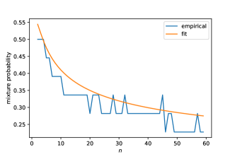
Following the above empirical procedure, we conclude the degrees of freedom ν𝜈\nu is not particularly important to the efficiency of the sampler, so we set it to 10. The mixture probability p𝑝p is important, however, and we fit a simple parametric curve to it:

0.100βˆ’0.486n+0.647n1/2+0.272n1/4.0.1000.486𝑛0.647superscript𝑛120.272superscript𝑛14\displaystyle 0.100-\frac{0.486}{n}+\frac{0.647}{n^{1/2}}+\frac{0.272}{n^{1/4}}. (26)

The empirical results and this simple fit are shown in Figure 1. Note that our parametric fit is monotonically decreasing, which is intuitively appropriate as the tails of ρnsubscriptπœŒπ‘›\rho_{n} lighten as n𝑛n increases.

Refer to caption
Figure 1: Empirical results for the optimal mixture probability with respect to the best attainable acceptance probability in the rejection sampler for ρnsubscriptπœŒπ‘›\rho_{n}.

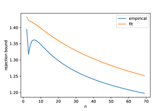
Now fixing the form of the mixture probability in (26), we numerically find approximations to the tightest bounds Mnsubscript𝑀𝑛M_{n}. Practically, this is done by evaluating the ratio ρn/hp,Ξ½subscriptπœŒπ‘›subscriptβ„Žπ‘πœˆ\rho_{n}/h_{p,\nu} over (βˆ’2​nβˆ’10,2​n+10)2𝑛102𝑛10(-2\sqrt{n}-10,2\sqrt{n}+10) on a finely-spaced grid and taking the maximum. We then fit a parametric form to the resulting data, building in some extra tolerance to ensure that our parametric fit is certainly a uniform upper bound for ρn/fp,Ξ½subscriptπœŒπ‘›subscriptπ‘“π‘πœˆ\rho_{n}/f_{p,\nu}. The results are shown in Figure 4 and the parametric fit is

0.492+1.058nβˆ’3.352n1/2+3.308n1/4.0.4921.058𝑛3.352superscript𝑛123.308superscript𝑛14\displaystyle 0.492+\frac{1.058}{n}-\frac{3.352}{n^{1/2}}+\frac{3.308}{n^{1/4}}. (27)
Refer to caption
Figure 2: Empirical results for the tightest uniform rejection bound on ρn/fp,Ξ½subscriptπœŒπ‘›subscriptπ‘“π‘πœˆ\rho_{n}/f_{p,\nu}.

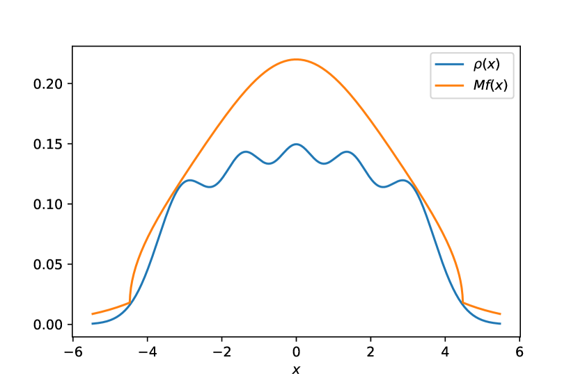
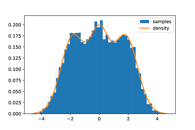
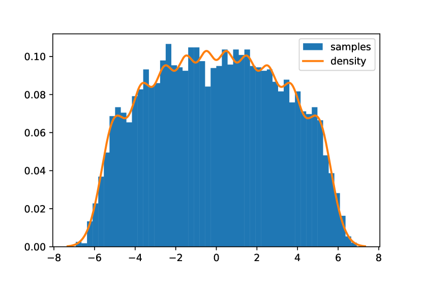
Figure 3 shows the target density ρnsubscriptπœŒπ‘›\rho_{n} and the scaled proposal density Mn​hpn,Ξ½subscript𝑀𝑛subscriptβ„Žsubscriptπ‘π‘›πœˆM_{n}h_{p_{n},\nu}. We show some results of using our rejection sampler for ρnsubscriptπœŒπ‘›\rho_{n} for various n𝑛n in Figure 4.

Refer to caption
(a) n=3𝑛3n=3
Refer to caption
(b) n=5𝑛5n=5
Refer to caption
(c) n=10𝑛10n=10
Figure 3: Comparison of the target density ρnsubscriptπœŒπ‘›\rho_{n} and the scaled proposal density Mn​fpn,Ξ½subscript𝑀𝑛subscript𝑓subscriptπ‘π‘›πœˆM_{n}f_{p_{n},\nu} for various n𝑛n values.
Refer to caption
(a) n=3𝑛3n=3
Refer to caption
(b) n=5𝑛5n=5
Refer to caption
(c) n=10𝑛10n=10
Figure 4: Results of using our rejection sampler for ρnsubscriptπœŒπ‘›\rho_{n} for a few different n𝑛n values. We used 10000 samples and 50 histogram bins.

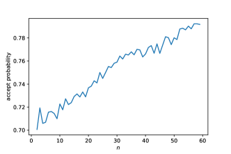
Finally, fixing our parametric fits, we can estimate the actual obtained acceptance probability. The results from 10000 trials for each n𝑛n value are shown in Figure 5. Note that the acceptance probability is generally increasing in n𝑛n and never less that 0.70.70.7.

Refer to caption
Figure 5: The empirically obtained acceptance probability for the rejection sampler of ρnsubscriptπœŒπ‘›\rho_{n} for various n𝑛n values. Calculated from 10000 trials.

2.2 Extension to rejection sampler in the general case

In the previous subsection we restricted to an extremely special case N=nd𝑁superscript𝑛𝑑N=n^{d}. In this section we leverage the sampler we constructed in that case to construct one for general N𝑁N.

Given Nβˆˆβ„•π‘β„•N\in\mathbb{N}, and dimension d>1𝑑1d>1, define n=⌈N1/dβŒ‰π‘›superscript𝑁1𝑑n=\lceil N^{1/d}\rceil and define also m=ndβˆ’Nπ‘šsuperscript𝑛𝑑𝑁m=n^{d}-N. Note that 0≀m≀ndβˆ’(nβˆ’1)dβˆ’10π‘šsuperscript𝑛𝑑superscript𝑛1𝑑10\leq m\leq n^{d}-(n-1)^{d}-1. Define

qn​(𝒙)=1nd​d​μ​(𝒙)β€‹βˆ‘π”Ÿβ€‹(π’Š)=0ndβˆ’1Ο•π’Šβ€‹(𝒙)2subscriptπ‘žπ‘›π’™1superscriptπ‘›π‘‘π‘‘πœ‡π’™superscriptsubscriptπ”Ÿπ’Š0superscript𝑛𝑑1subscriptitalic-Ο•π’Šsuperscript𝒙2\displaystyle q_{n}(\bm{x})=\frac{1}{n^{d}}d\mu(\bm{x})\sum_{\mathfrak{b}(\bm{i})=0}^{n^{d}-1}\phi_{\bm{i}}(\bm{x})^{2} (28)

and then we can immediately write down the bound

fN​(𝒙)qn​(𝒙)=1N​d​μ​(𝒙)β€‹βˆ‘π”Ÿβ€‹(π’Š)=0Nβˆ’1Ο•π’Šβ€‹(𝒙)21nd​d​μ​(𝒙)β€‹βˆ‘π”Ÿβ€‹(π’Š)=0ndβˆ’1Ο•π’Šβ€‹(𝒙)2≀ndndβˆ’m.subscript𝑓𝑁𝒙subscriptπ‘žπ‘›π’™1π‘π‘‘πœ‡π’™superscriptsubscriptπ”Ÿπ’Š0𝑁1subscriptitalic-Ο•π’Šsuperscript𝒙21superscriptπ‘›π‘‘π‘‘πœ‡π’™superscriptsubscriptπ”Ÿπ’Š0superscript𝑛𝑑1subscriptitalic-Ο•π’Šsuperscript𝒙2superscript𝑛𝑑superscriptπ‘›π‘‘π‘š\displaystyle\frac{f_{N}(\bm{x})}{q_{n}(\bm{x})}=\frac{\frac{1}{N}d\mu(\bm{x})\sum_{\mathfrak{b}(\bm{i})=0}^{N-1}\phi_{\bm{i}}(\bm{x})^{2}}{\frac{1}{n^{d}}d\mu(\bm{x})\sum_{\mathfrak{b}(\bm{i})=0}^{n^{d}-1}\phi_{\bm{i}}(\bm{x})^{2}}\leq\frac{n^{d}}{n^{d}-m}. (29)

Sampling from qnsubscriptπ‘žπ‘›q_{n} can be achieved using the factorised rejection sampler derived in the previous subsection, so we have all that is required for a rejection sampler for fNsubscript𝑓𝑁f_{N} for general N𝑁N.

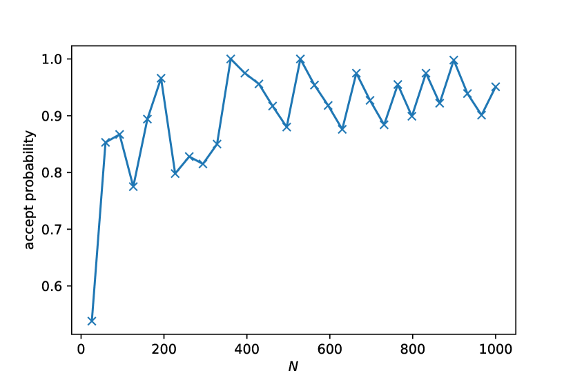
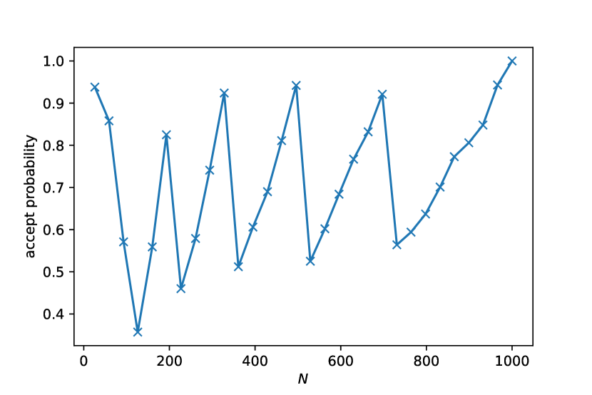
Figure 6 shows empirical acceptance probabilities for dimension 2,3232,3 and 444 over a range of N𝑁N values. Note that these values are just for the rejection sampler described by (29), treating the rejection sampler for qπ‘žq as a black-box. Unsurprisingly the acceptance probability has some oscillatory behaviour in N𝑁N, with the peaks corresponding to perfect powers of d𝑑d, followed by sharp drops as mπ‘šm jumps from its best value of 00 to its worst of ndβˆ’1superscript𝑛𝑑1n^{d}-1. That being said, the acceptance probabilities are still very good for d=2𝑑2d=2 above around N=100𝑁100N=100. For smaller values of N𝑁N the acceptance probabilities are still good enough, particularly as the other components of the DPP sampler become cheaper with decreasing N𝑁N. d=3,4𝑑34d=3,4 also appear feasible, though clearly less efficient that d=2𝑑2d=2. Higher values of d𝑑d are also plausible, though the scaling with d𝑑d is clearly poor (c.f. [4, 6] where the acceptance probability scales like 2βˆ’dsuperscript2𝑑2^{-d}.)

Refer to caption
(a) d=2𝑑2d=2
Refer to caption
(b) d=3𝑑3d=3
Refer to caption
(c) d=4𝑑4d=4
Figure 6: Empirical acceptance probabilities for the general N𝑁N sampler constructed in Section 2.2. 1000 trials are used for each N𝑁N values.

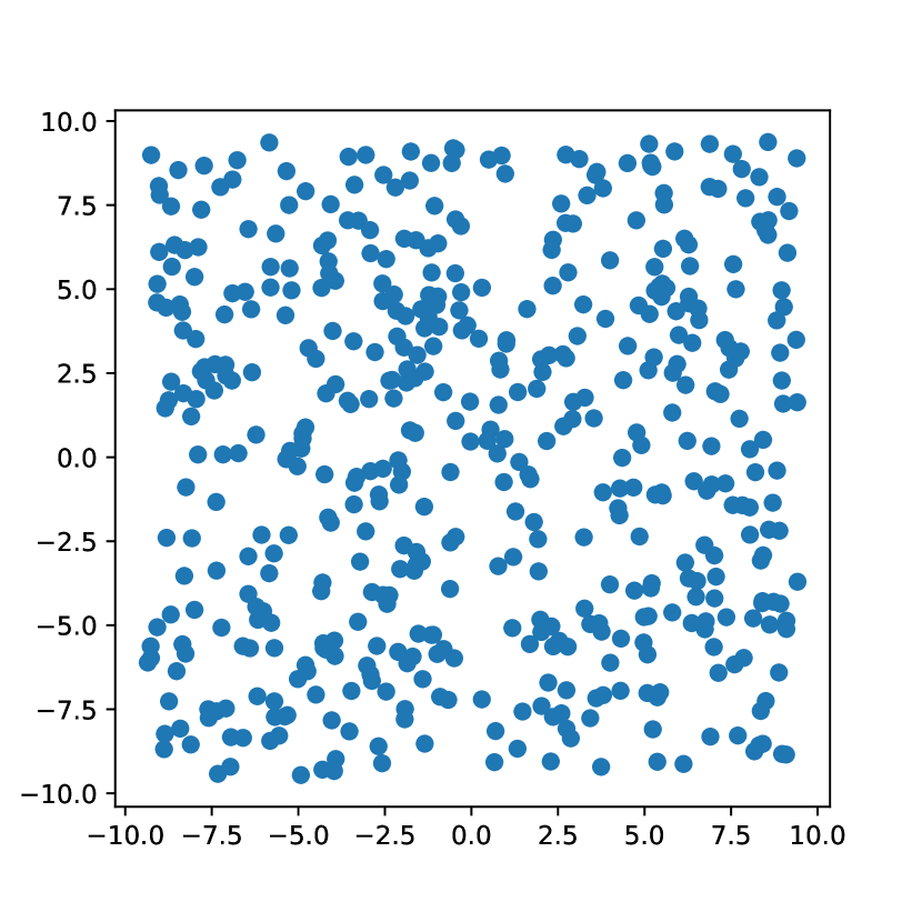
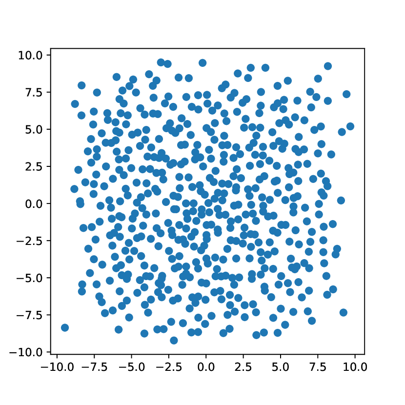
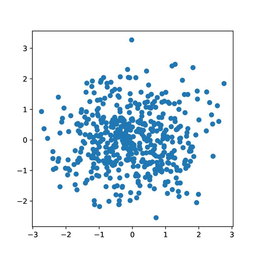
Figure 7 show a sample from the constructed Gauss-Hermite DPP in 2 dimension and with 500 points. For comparison we also show a sample from the base measure, a standard Gaussian in 2 dimensions, and from a Poisson process on (βˆ’2​N1/4,2​N1/4)2superscript𝑁142superscript𝑁14(-2N^{1/4},2N^{1/4}) (the domain in which the DPP has the vast majority of its support). The effect of the DPP repulsion is evident when comparing it to the base measure, as the points have filled a much larger domain. The repulsion is also evident when comparing the DPP to the Poisson process. The two processes have produced points in very similar domains, but the DPP shows much more uniformity of placement, with the Poisson process showing lots of characteristic clustering of points.
Refer to caption
(a) DPP​(ΞΌ,KN)DPPπœ‡subscript𝐾𝑁\text{DPP}(\mu,K_{N})
Refer to caption
(b) i.i.d. Gaussian
Refer to caption
(c) Poisson process
Figure 7: Samples in 2 dimension with N=500𝑁500N=500. We show the DPP and for comparison i.i.d. samples from the base Gaussian measure and also a Poisson process on (βˆ’2​N1/4,2​N1/4)2superscript𝑁142superscript𝑁14(-2N^{1/4},2N^{1/4}).

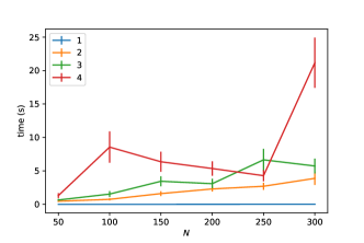
Figure 8 shows some timing results for the DPP sampler in dimensions d=1,2,3,4𝑑1234d=1,2,3,4. The results are broadly similar to those of [4], which is unsurprising since the top-level chain rule step of the sampler is the same and the lower-level rejection samplers are efficient in both cases for small d𝑑d. Our rejection sampler for fNsubscript𝑓𝑁f_{N} introduces rN,dβˆ’1​d​s⌈N1/dβŒ‰βˆ’1superscriptsubscriptπ‘Ÿπ‘π‘‘1𝑑subscriptsuperscript𝑠1superscript𝑁1𝑑r_{N,d}^{-1}ds^{-1}_{\lceil N^{1/d}\rceil}, where snsubscript𝑠𝑛s_{n} is the acceptance probability for our sampler of ρnsubscriptπœŒπ‘›\rho_{n}, so snβ‰₯0.7subscript𝑠𝑛0.7s_{n}\geq 0.7, and rN,dsubscriptπ‘Ÿπ‘π‘‘r_{N,d} is the acceptance probability for our overall rejection sampler for fNsubscript𝑓𝑁f_{N}, so it appears rN,dβ‰₯0.4subscriptπ‘Ÿπ‘π‘‘0.4r_{N,d}\geq 0.4 for Nβ‰₯200𝑁200N\geq 200 and with most N𝑁N values having much better values. Comparing the figure to the corresponding one in [4] does suggest that for d=4𝑑4d=4 our rejection sampler for fNsubscript𝑓𝑁f_{N} is introducing extra inefficiency beyond that of the top-level chain-rule sampler. However, recalling the acceptance probabilities in Figure 6, it appears that the poorer performance of for d=4𝑑4d=4 is caused by the complexity of computing many more Hermite polynomial evaluations, namely (⌈N1/dβŒ‰)dsuperscriptsuperscript𝑁1𝑑𝑑(\lceil N^{1/d}\rceil)^{d} rather than just N𝑁N. This is encouraging, as the best case scenario (as achieved by [4] in the Jacobi case) requires evaluation of the first N1/dsuperscript𝑁1𝑑N^{1/d} Hermite polynomials. Our sampling strategy required ⌈N1/dβŒ‰superscript𝑁1𝑑\lceil N^{1/d}\rceil which is of the same order of complexity for large N𝑁N.

Refer to caption
Figure 8: The wall-time of sampling from DPP​(ΞΌ,KN)DPPπœ‡subscript𝐾𝑁\text{DPP}(\mu,K_{N}) for various dimensions 1,2,3,412341,2,3,4 and a range of N𝑁N values. Shown are means and one standard deviation either side over 30 repeated samplings for each N𝑁N and d𝑑d.

3 Application to Monte Carlo integration

In [4] the authors present two DPP-based Monte Carlo (MC) integration schemes (BH and EZ) for integrals of the from

∫[βˆ’1,1]d𝑑μ​(𝒙)​f​(𝒙)subscriptsuperscript11𝑑differential-dπœ‡π’™π‘“π’™\displaystyle\int_{[-1,1]^{d}}d\mu(\bm{x})f(\bm{x}) (30)

where ΞΌπœ‡\mu is multivariate Jacobi measure on [βˆ’1,1]dsuperscript11𝑑[-1,1]^{d}. Armed with our multivariate Gauss-Hermite DPP, we can also apply their methods to integrals of the form

βˆ«β„d𝑑μ​(𝒙)​f​(𝒙)subscriptsuperscriptℝ𝑑differential-dπœ‡π’™π‘“π’™\displaystyle\int_{\mathbb{R}^{d}}d\mu(\bm{x})f(\bm{x}) (31)

where recall d​μ​(𝒙)=eβˆ’π’™22​dβ€‹π’™π‘‘πœ‡π’™superscript𝑒superscript𝒙22𝑑𝒙d\mu(\bm{x})=e^{-\frac{\bm{x}^{2}}{2}}d\bm{x}. Moreover, given some mean 𝝁𝝁\bm{\mu} and covariance matrix 𝚺𝚺\bm{\Sigma} we have

βˆ«β„d𝑑𝒙​𝒩​(𝒙;𝝁,𝚺)​f​(𝒙)subscriptsuperscriptℝ𝑑differential-dπ’™π’©π’™ππšΊπ‘“π’™\displaystyle\int_{\mathbb{R}^{d}}d\bm{x}\leavevmode\nobreak\ \mathcal{N}(\bm{x};\bm{\mu},\bm{\Sigma})f(\bm{x}) =1(2​π)d/2β€‹βˆ«β„d𝑑μ​(𝒙)​f​(𝚺1/2​𝒙+𝝁)absent1superscript2πœ‹π‘‘2subscriptsuperscriptℝ𝑑differential-dπœ‡π’™π‘“superscript𝚺12𝒙𝝁\displaystyle=\frac{1}{(2\pi)^{d/2}}\int_{\mathbb{R}^{d}}d\mu(\bm{x})f(\bm{\Sigma}^{1/2}\bm{x}+\bm{\mu}) (32)

and so estimation of integrals against any Gaussian probability measure is possible by the reparametrisation trick. Other than switching to our Gauss-Hermite DPP from the Jacobi DPP, we make no other changes to the BH and EZ approaches.

3.1 Perfect esimation of polynomials

Consider functions ℝd→ℝ→superscriptℝ𝑑ℝ\mathbb{R}^{d}\rightarrow\mathbb{R} of the form

f​(x)=βˆ‘i1,…,id=1paπ’Šβ€‹βˆk=1dxkik𝑓π‘₯superscriptsubscriptsubscript𝑖1…subscript𝑖𝑑1𝑝subscriptπ‘Žπ’Šsuperscriptsubscriptproductπ‘˜1𝑑superscriptsubscriptπ‘₯π‘˜subscriptπ‘–π‘˜\displaystyle f(x)=\sum_{i_{1},\ldots,i_{d}=1}^{p}a_{\bm{i}}\prod_{k=1}^{d}x_{k}^{i_{k}} (33)

where aπ’Šsubscriptπ‘Žπ’Ša_{\bm{i}} are coefficients. The integral of f𝑓f against Gaussian measure is simple to compute:

βˆ«β„d𝑑𝒙​𝒩​(𝒙;𝝁,𝚺)​f​(𝒙)=βˆ‘i1,…,id=1paπ’Šβ€‹βˆk=1dβˆ«β„π‘‘x​eβˆ’x222​π​xkik=βˆ‘i1,…,id=1paπ’Šβ€‹βˆk=1dm​(ik)subscriptsuperscriptℝ𝑑differential-dπ’™π’©π’™ππšΊπ‘“π’™superscriptsubscriptsubscript𝑖1…subscript𝑖𝑑1𝑝subscriptπ‘Žπ’Šsuperscriptsubscriptproductπ‘˜1𝑑subscriptℝdifferential-dπ‘₯superscript𝑒superscriptπ‘₯222πœ‹superscriptsubscriptπ‘₯π‘˜subscriptπ‘–π‘˜superscriptsubscriptsubscript𝑖1…subscript𝑖𝑑1𝑝subscriptπ‘Žπ’Šsuperscriptsubscriptproductπ‘˜1π‘‘π‘šsubscriptπ‘–π‘˜\displaystyle\int_{\mathbb{R}^{d}}d\bm{x}\leavevmode\nobreak\ \mathcal{N}(\bm{x};\bm{\mu},\bm{\Sigma})f(\bm{x})=\sum_{i_{1},\ldots,i_{d}=1}^{p}a_{\bm{i}}\prod_{k=1}^{d}\int_{\mathbb{R}}dx\leavevmode\nobreak\ \frac{e^{-\frac{x^{2}}{2}}}{\sqrt{2\pi}}x_{k}^{i_{k}}=\sum_{i_{1},\ldots,i_{d}=1}^{p}a_{\bm{i}}\prod_{k=1}^{d}m(i_{k}) (34)

where m​(i)=(iβˆ’1)!!π‘šπ‘–double-factorial𝑖1m(i)=(i-1)!! if i𝑖i even and m​(i)=0π‘šπ‘–0m(i)=0 otherwise.

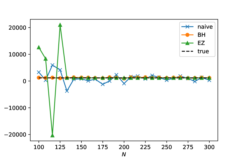
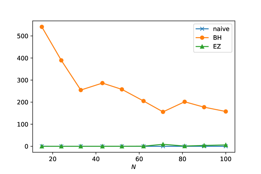
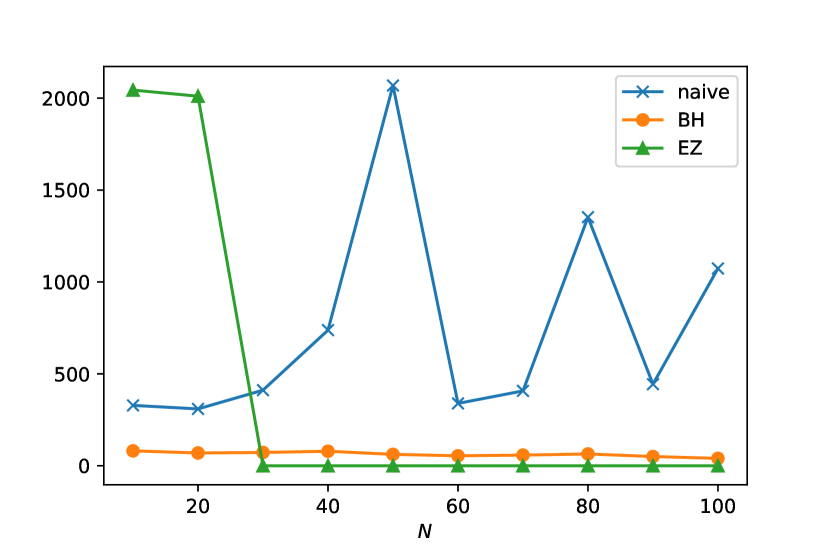
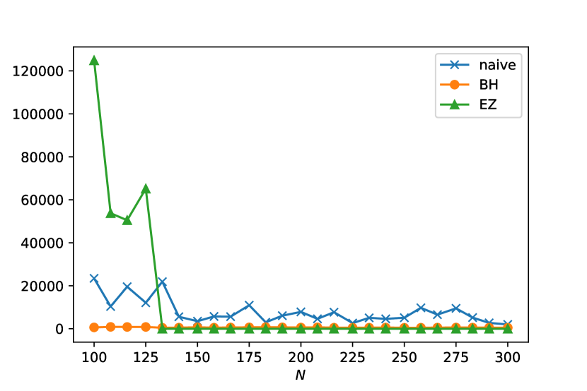
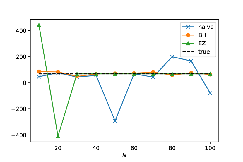
Figure 9 shows the results of using the BH, EZ and naΓ―ve MC integration approaches. We show the mean and standard deviation over 30 repeated samples. The polynomial are selected at random but are kept fixed throughout. The degree of the polynomials is 10 for d=1𝑑1d=1, 5 for d=2,3𝑑23d=2,3. The reduction in degree for higher dimension is necessary to prevent the true values given by (34) from becoming unreasonably large.

Refer to caption
Refer to caption
Refer to caption
Refer to caption
(a) d=1𝑑1d=1
Refer to caption
(b) d=2𝑑2d=2
Refer to caption
(c) d=3𝑑3d=3
Figure 9: Result of MC integration on multivariate polynomials using Gauss-Hermite DPPs and comparing the naΓ―ve MC approach to the BH and EZ approaches. The top row shows the sample means over 30 repetitions and the bottom row shows the sample standard deviation.

The results generally accord with those of [4], with the the EZ estimator performing best but become less reliable with increasing d𝑑d, in particular prone to ill-conditioning leading to enormous outliers. The BH estimator becomes more favourable with increasing dimension. All estimators benefit from increasing sample size N𝑁N, but the EZ estimator benefits most dramatically. For example in the d=2𝑑2d=2 case the EZ estimator is very poor until around N=30𝑁30N=30 when, beyond which it recovers the true value with zero variance (perfect estimation). This can be explained as follows: we chose a degree 555 polynomial. For N<25𝑁25N<25, the kernel KNsubscript𝐾𝑁K_{N} includes only multivariate Hermite polynomials of at most degree 444, hence the chosen polynomial is not in the span of the RKHS basis.

3.2 Marginalised Gaussian process posteriors

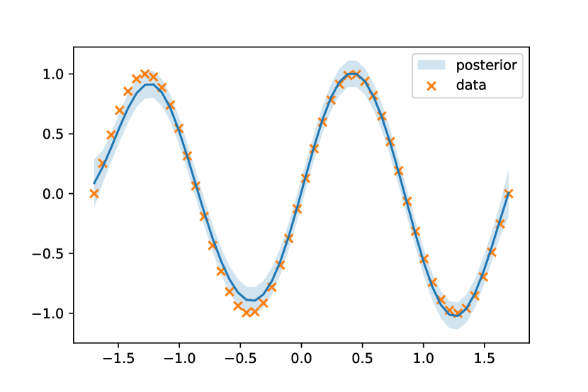
Here we will consider a Gaussian process (GP) posterior on a simple synthetic dataset. The synthetic data are just draw from a one dimensional sine wave and are shown in Figure 10(a). We will use a simple scaled radial basis function (RBF) kernel without automatic relevance determination:

k​(x,xβ€²)=v​exp⁑(βˆ’(xβˆ’x)2l2)π‘˜π‘₯superscriptπ‘₯′𝑣superscriptπ‘₯π‘₯2superscript𝑙2k(x,x^{\prime})=v\exp\left(-\frac{(x-x)^{2}}{l^{2}}\right)

where v>0𝑣0v>0 and l>0𝑙0l>0 are hyperparameters. In standard GP practice, the hyperparameters v,l𝑣𝑙v,l are optimised as point estimates by maximising the log marginal likelihood of the training data under the model. To enforce the positivity constrains on v,l𝑣𝑙v,l we adopt the standard practice (used e.g. by GPyTorch [10]) of writing them as softplus transforms of raw hyperparameters:

v=log⁑(exp⁑(ΞΈ1)+1),l=log⁑(exp⁑(ΞΈ2)+1).formulae-sequence𝑣subscriptπœƒ11𝑙subscriptπœƒ21\displaystyle v=\log(\exp(\theta_{1})+1),\leavevmode\nobreak\ \leavevmode\nobreak\ \leavevmode\nobreak\ l=\log(\exp(\theta_{2})+1). (35)

In Bayesian treatments of GP hyperparameters, one promotes a point estimate of ΞΈπœƒ\theta to a full posterior distribution (see e.g. [11]). Further pursuit of such ideas is well outside the scope of this paper, however it suffices to note that a Gaussian form of the posterior is the most practical choice (e.g. as in Variational inference approaches [11]). We will place a Gaussian over the raw hyperparameters ΞΈπœƒ\theta. For demonstration purposes, we will take a unit variance factorised Gaussian centred on the point-estimate raw-hyperparameters from applying marginal likelihood maximisation.333This is not dissimilar to a Laplace approximation of a posterior over the hyperparameters, though the variance is certainly not correct. We will consider a simple 1-dimensional index space and a simple single-output regression problem on synthetic data.

We now seek the hyperparameter-marginalised GP posterior confidence intervals. The point-wise CDF is

Ψ​(y)=βˆ«π‘‘ΞΈβ€‹Ξ¦β€‹(yβˆ’ΞΌβ€‹(ΞΈ+ΞΈβˆ—)σ​(ΞΈ+ΞΈβˆ—))​eβˆ’ΞΈ222​πΨ𝑦differential-dπœƒΞ¦π‘¦πœ‡πœƒsubscriptπœƒπœŽπœƒsubscriptπœƒsuperscript𝑒superscriptπœƒ222πœ‹\displaystyle\Psi(y)=\int d\theta\leavevmode\nobreak\ \Phi\left(\frac{y-\mu(\theta+\theta_{*})}{\sigma(\theta+\theta_{*})}\right)\frac{e^{-\frac{\theta^{2}}{2}}}{2\pi} (36)

where ΞΈβˆ—subscriptπœƒ\theta_{*} is the centre of the raw-hyperparameter Gaussian obtained from MLL maximisation, ΞΌ,Οƒπœ‡πœŽ\mu,\sigma are the point-wise posterior mean and standard deviation of the GP posterior as a function of ΞΈπœƒ\theta, and ΦΦ\Phi is the standard Gaussian CDF. There is an implicit dependence throughout on the index point xπ‘₯x. We then seek y2=Ξ¨βˆ’1​(0.975),y1=Ξ¨βˆ’1​(0.025)formulae-sequencesubscript𝑦2superscriptΞ¨10.975subscript𝑦1superscriptΞ¨10.025y_{2}=\Psi^{-1}(0.975),\leavevmode\nobreak\ y_{1}=\Psi^{-1}(0.025), the boundaries of a confidence interval. Rather than embarking on numerical inversion of ΨΨ\Psi, we will opt for simpler heuristics that nevertheless demonstrate the DPP MC integration methods, which is our objective. We compute

ΞΌΒ―=βˆ«π‘‘ΞΈβ€‹eβˆ’ΞΈ222​π​μ​(ΞΈ+ΞΈβˆ—)Β―πœ‡differential-dπœƒsuperscript𝑒superscriptπœƒ222πœ‹πœ‡πœƒsubscriptπœƒ\displaystyle\bar{\mu}=\int d\theta\leavevmode\nobreak\ \frac{e^{-\frac{\theta^{2}}{2}}}{2\pi}\mu(\theta+\theta_{*}) (37)

and

σ¯=βˆ«π‘‘ΞΈβ€‹eβˆ’ΞΈ222​π​σ​(ΞΈ+ΞΈβˆ—).¯𝜎differential-dπœƒsuperscript𝑒superscriptπœƒ222πœ‹πœŽπœƒsubscriptπœƒ\displaystyle\bar{\sigma}=\int d\theta\leavevmode\nobreak\ \frac{e^{-\frac{\theta^{2}}{2}}}{2\pi}\sigma(\theta+\theta_{*}). (38)

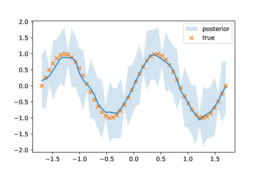
These yield confidence intervals (ΞΌΒ―βˆ’1.96​σ¯,ΞΌΒ―+1.96​σ¯)Β―πœ‡1.96Β―πœŽΒ―πœ‡1.96¯𝜎(\bar{\mu}-1.96\bar{\sigma},\bar{\mu}+1.96\bar{\sigma}), which are certainly not the posterior 95%percent9595\% confidence intervals of the marginalised GP, but are perhaps not dissimilar in some cases. Figure 10 shows the point estimate posterior on a test set alongside the same EZ marginalised pseudo posterior. We note merely that the increased posterior uncertainty appears reasonable and also that the BH and naΓ―ve plots are very similar, but with slightly higher variance in the naΓ―ve case.

Refer to caption
(a) Point estimate.
Refer to caption
(b) EZ marginalised.
Figure 10: Marginalised GP posterior using EZ MC integration to compute ΞΌΒ―Β―πœ‡\bar{\mu} and ΟƒΒ―Β―πœŽ\bar{\sigma}. The shaded region in (b) shows (ΞΌΒ―βˆ’1.96​σ¯,ΞΌΒ―+1.96​σ¯)Β―πœ‡1.96Β―πœŽΒ―πœ‡1.96¯𝜎(\bar{\mu}-1.96\bar{\sigma},\bar{\mu}+1.96\bar{\sigma}), whereas the shaded region in (a) is the standard posterior 95%percent9595\% confindence interval for the point estimate GP.

To really test the utility of our DPP MC integration approaches in this case, we must assess the accuracy of estimation of the CDF ΨΨ\Psi defined in (36). To this end, for all xπ‘₯x values in the test set, we compute Ψ​(y)Ψ𝑦\Psi(y) for each

y∈{ΞΌΒ―βˆ’4​σ¯,ΞΌΒ―βˆ’1.96​σ¯,ΞΌΒ―βˆ’ΟƒΒ―,ΞΌΒ―,ΞΌΒ―+σ¯,ΞΌΒ―+1.96​σ¯,ΞΌΒ―+4​σ¯}.π‘¦Β―πœ‡4Β―πœŽΒ―πœ‡1.96Β―πœŽΒ―πœ‡Β―πœŽΒ―πœ‡Β―πœ‡Β―πœŽΒ―πœ‡1.96Β―πœŽΒ―πœ‡4¯𝜎\displaystyle y\in\{\bar{\mu}-4\bar{\sigma},\bar{\mu}-1.96\bar{\sigma},\bar{\mu}-\bar{\sigma},\bar{\mu},\bar{\mu}+\bar{\sigma},\bar{\mu}+1.96\bar{\sigma},\bar{\mu}+4\bar{\sigma}\}. (39)

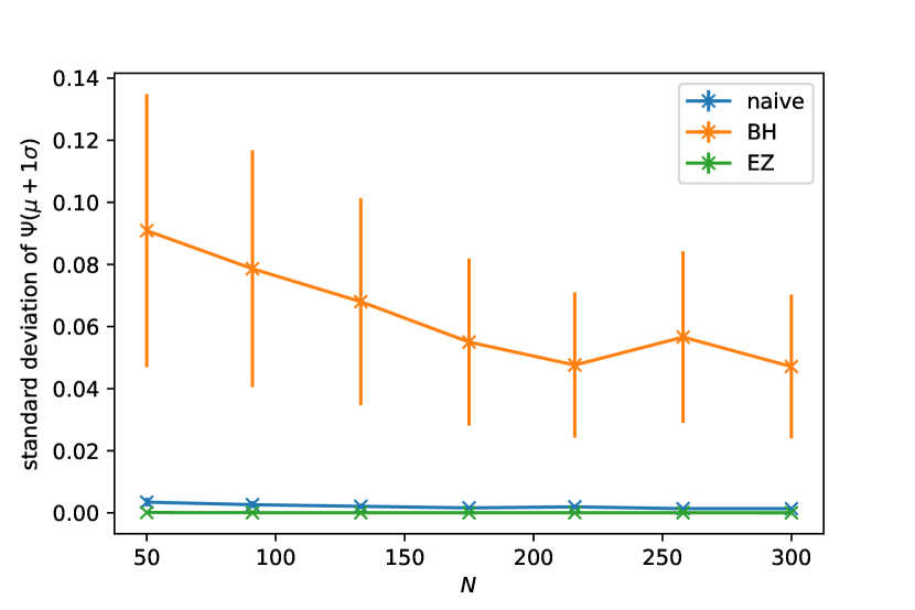
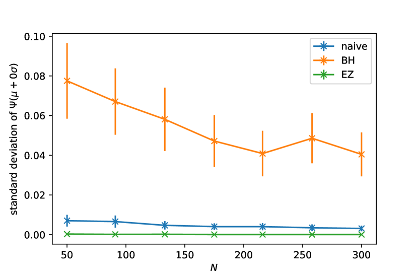
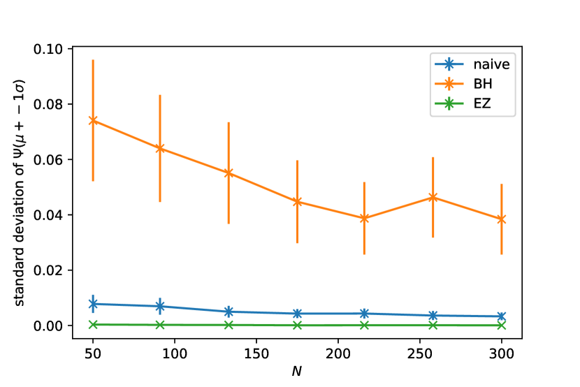
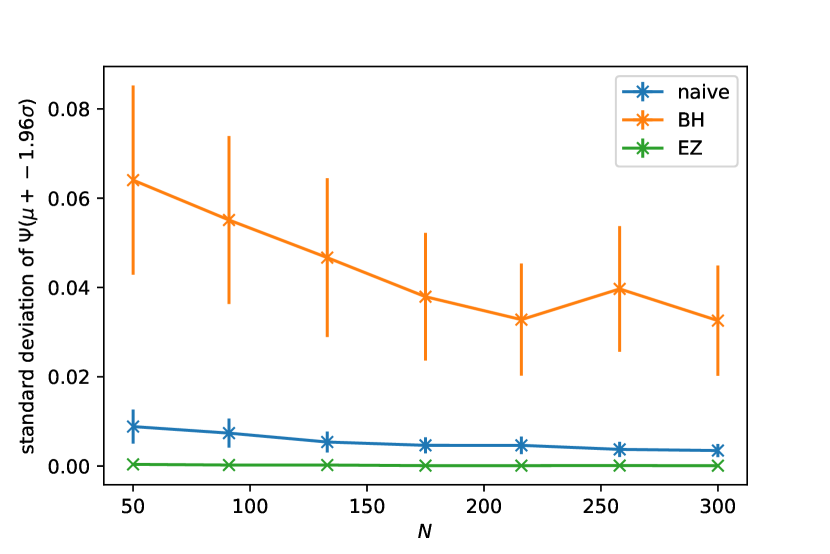
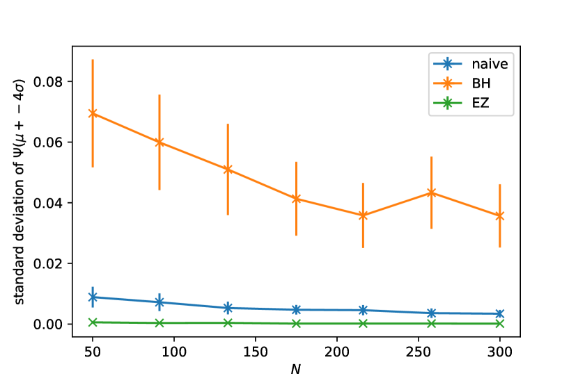
Accurate estimation of such values is critical for accurate estimation of confidence intervals. We repeat this estimation 30 times (resampling the DPP/i.i.d. sample points) leading to 30 values for each of the 7 y𝑦y values at each of the 50 test points. To visualise, we then compute the sample standard deviation over the 30 re-samplings, leading to 7Γ—507507\times 50 standard deviation values of which we take the sample mean over the 50 points. Figure 11 shows the resulting standard deviation values for each of the 7 y𝑦y values and each of the estimators. The results show, perhaps surprisingly, EZ outperforming BH and naΓ―ve in all cases. This indicates that the GP posterior CDF has rapidly decaying coefficients in an Hermite polynomial expansion [4].
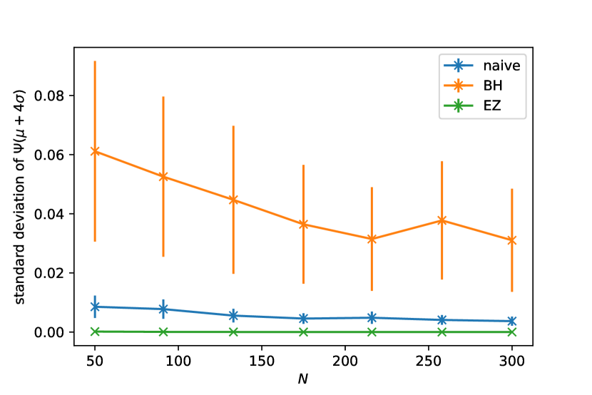
Refer to caption
(a) y=ΞΌΒ―βˆ’4β€‹ΟƒΒ―π‘¦Β―πœ‡4¯𝜎y=\bar{\mu}-4\bar{\sigma}
Refer to caption
(b) y=ΞΌΒ―βˆ’1.96β€‹ΟƒΒ―π‘¦Β―πœ‡1.96¯𝜎y=\bar{\mu}-1.96\bar{\sigma}
Refer to caption
(c) y=ΞΌΒ―βˆ’ΟƒΒ―π‘¦Β―πœ‡Β―πœŽy=\bar{\mu}-\bar{\sigma}
Refer to caption
(d) y=ΞΌΒ―π‘¦Β―πœ‡y=\bar{\mu}
Refer to caption
(e) y=ΞΌΒ―+ΟƒΒ―π‘¦Β―πœ‡Β―πœŽy=\bar{\mu}+\bar{\sigma}
Refer to caption
(f) y=ΞΌΒ―+1.96β€‹ΟƒΒ―π‘¦Β―πœ‡1.96¯𝜎y=\bar{\mu}+1.96\bar{\sigma}
Refer to caption
(g) y=ΞΌΒ―+4β€‹ΟƒΒ―π‘¦Β―πœ‡4¯𝜎y=\bar{\mu}+4\bar{\sigma}
Figure 11: Estimating the GP CDF ΨΨ\Psi defined in (36). Each plot shows results for naΓ―ve, BC and EZ estimators using a range of sample sizes. We plot the standard deviation of the estimates over resampling of the DPP/i.i.d. points. The error bars show standard deviation over the 50 GP evaluation points. Each subfigure considers a different y𝑦y value in Ψ​(y)Ψ𝑦\Psi(y).

4 Conclusions and future work

We have considered multivariate Hermite polynomials for the construction of determinantal points processes with Gaussian base measure. To enable their practical use, we have developed a novel multi-stage sampler for such Gauss-Hermite DPPs that is quite different from prior analogous samplers for other DPPs. Our experimental timing and efficiency results demonstrate that the sampler is practically feasible and in-line with performance obtained by prior DPP samplers. We have presented some experimental results using Gauss-Hermite DPPs in BH and EZ approaches to MC integration, showing strong performance in a variety of tasks. In particular, we have presented some novel experimental results using Gauss-Hermite DPPs and BH/EZ estimation to marginalise the hyperparameters of a Gaussian process regression posterior. The excellent results of the EZ estimator in this case suggest that the GP posterior, as functions of the raw hyperparameters, are well adapted to the Hermite basis. We remark that the factorised form (15) of the DPP posterior is clearly related to the posterior covariance of a Gaussian process with kernel KNsubscript𝐾𝑁K_{N}. It would be interesting to consider if this similarity could be in part responsible for the excellent EZ performance, perhaps suggesting that EZ MC integration is particularly suited to GP posteriors. Future work should also consider optimising the implementations to avoid repeated Hermite polynomials evaluations, in particular evaluations used in sampling from the top-level proposal density fNsubscript𝑓𝑁f_{N} could be recycled for use in evaluating the acceptance ratio itself. Finally, we constructed an empirically optimised rejection sampler for the univariate truncated Hermite mixtures ρnsubscriptπœŒπ‘›\rho_{n} being inspired by the convergence of such distributions to the Wigner semi-circle law. This leaves open the question of obtaining analytically rejection bounds, and in particular bounds that are good enough for practical use in the rejection sampler. We have not been able to derive such bounds, but the semi-circle convergence does suggest that they might be available.

References

  • [1] M.Β L. Mehta, Random matrices. Elsevier, 2004.
  • [2] G.Β Livan, M.Β Novaes, and P.Β Vivo, Introduction to random matrices: theory and practice, vol.Β 26. Springer, 2018.
  • [3] J.Β B. Hough, M.Β Krishnapur, Y.Β Peres, and B.Β VirΓ‘g, β€œDeterminantal processes and independence,” Probability surveys, vol.Β 3, pp.Β 206–229, 2006.
  • [4] G.Β Gautier, R.Β Bardenet, and M.Β Valko, β€œOn two ways to use determinantal point processes for monte carlo integration,” in Advances in Neural Information Processing Systems (H.Β Wallach, H.Β Larochelle, A.Β Beygelzimer, F.Β d'AlchΓ©-Buc, E.Β Fox, and R.Β Garnett, eds.), vol.Β 32, Curran Associates, Inc., 2019.
  • [5] A.Β Kulesza and B.Β Taskar, β€œDeterminantal point processes for machine learning,” arXiv preprint arXiv:1207.6083, 2012.
  • [6] R.Β Bardenet and A.Β Hardy, β€œMonte carlo with determinantal point processes,” The Annals of Applied Probability, vol.Β 30, no.Β 1, pp.Β 368–417, 2020.
  • [7] S.Β M. Ermakov and V.Β Zolotukhin, β€œPolynomial approximations and the monte-carlo method,” Theory of Probability & Its Applications, vol.Β 5, no.Β 4, pp.Β 428–431, 1960.
  • [8] I.Β Krasikov, β€œNew bounds on the hermite polynomials,” arXiv preprint math/0401310, 2004.
  • [9] G.Β W. Anderson, A.Β Guionnet, and O.Β Zeitouni, An introduction to random matrices. No.Β 118, Cambridge university press, 2010.
  • [10] J.Β R. Gardner, G.Β Pleiss, D.Β Bindel, K.Β Q. Weinberger, and A.Β G. Wilson, β€œGpytorch: Blackbox matrix-matrix gaussian process inference with gpu acceleration,” in Advances in Neural Information Processing Systems, 2018.
  • [11] V.Β Lalchand and C.Β E. Rasmussen, β€œApproximate inference for fully bayesian gaussian process regression,” in Symposium on Advances in Approximate Bayesian Inference, pp.Β 1–12, PMLR, 2020.
  • [12] C.Β F. Dunkl and Y.Β Xu, Orthogonal polynomials of several variables. No.Β 155, Cambridge University Press, 2014.
  • [13] G.Β LohΓΆfer, β€œInequalities for legendre functions and gegenbauer functions,” Journal of Approximation Theory, vol.Β 64, no.Β 2, pp.Β 226–234, 1991.

Appendix A Gaussian orthonormal functions from spherical orthogonal functions

This section describes another novel construction of Guassian orthogonal function on ℝNsuperscriptℝ𝑁\mathbb{R}^{N} using spherical orthogonal functions. It is included for interest and to illustrate the difficulty of sampling from distributions of the form Ο•π’Šβ€‹(𝒙)​d​𝒙subscriptitalic-Ο•π’Šπ’™π‘‘π’™\phi_{\bm{i}(\bm{x})}d\bm{x} in the Gaussian case, as opposed to the Jacobi case of [4] which is well-behaved.

Suppose that {Οˆπ’}𝒏subscriptsubscriptπœ“π’π’\{\psi_{\bm{n}}\}_{\bm{n}} are a set of orthonormal functions defined on the d𝑑d-sphere (that is, the dβˆ’1𝑑1d-1 dimensional surface that is embedded in ℝdsuperscriptℝ𝑑\mathbb{R}^{d}). The multi-indices 𝒏𝒏\bm{n} are d𝑑d-tuples of non-negative integers. We have the defining orthonormality property:

∫Sd𝑑S​(𝒆)β€‹Οˆπ’β€‹(𝒆)β€‹Οˆπ’Žβ€‹(𝒆)=Ξ΄π’β€‹π’Ž,subscriptsuperscript𝑆𝑑differential-d𝑆𝒆subscriptπœ“π’π’†subscriptπœ“π’Žπ’†subscriptπ›Ώπ’π’Ž\int_{S^{d}}dS(\bm{e})\leavevmode\nobreak\ \psi_{\bm{n}}(\bm{e})\psi_{\bm{m}}(\bm{e})=\delta_{\bm{n}\bm{m}},

where d​S𝑑𝑆dS is the surface measure on the sphere. Let ΟƒdsubscriptπœŽπ‘‘\sigma_{d} be the surface area of the d𝑑d-sphere, then

βˆ«β„d𝑑𝒙​𝒩​(𝒙;0,Id)β€‹Οˆπ’β€‹(𝒙‖𝒙‖2)β€‹Οˆπ’Žβ€‹(𝒙‖𝒙‖2)=∫0βˆžπ‘‘r​rdβˆ’1​eβˆ’r22(2​π)d/2β€‹βˆ«Sd𝑑S​(𝒆)β€‹Οˆπ’β€‹(𝒆)β€‹Οˆπ’Žβ€‹(𝒆)=Οƒdβˆ’1β€‹Ξ΄π’β€‹π’Ž.subscriptsuperscriptℝ𝑑differential-d𝒙𝒩𝒙0subscript𝐼𝑑subscriptπœ“π’π’™subscriptnorm𝒙2subscriptπœ“π’Žπ’™subscriptnorm𝒙2superscriptsubscript0differential-dπ‘Ÿsuperscriptπ‘Ÿπ‘‘1superscript𝑒superscriptπ‘Ÿ22superscript2πœ‹π‘‘2subscriptsuperscript𝑆𝑑differential-d𝑆𝒆subscriptπœ“π’π’†subscriptπœ“π’Žπ’†superscriptsubscriptπœŽπ‘‘1subscriptπ›Ώπ’π’Ž\displaystyle\int_{\mathbb{R}^{d}}d\bm{x}\leavevmode\nobreak\ \mathcal{N}(\bm{x};0,I_{d})\psi_{\bm{n}}\left(\frac{\bm{x}}{\|\bm{x}\|_{2}}\right)\psi_{\bm{m}}\left(\frac{\bm{x}}{\|\bm{x}\|_{2}}\right)=\int_{0}^{\infty}dr\leavevmode\nobreak\ r^{d-1}\frac{e^{-\frac{r^{2}}{2}}}{(2\pi)^{d/2}}\int_{S^{d}}dS(\bm{e})\psi_{\bm{n}}(\bm{e})\psi_{\bm{m}}(\bm{e})=\sigma_{d}^{-1}\delta_{\bm{n}\bm{m}}.

Define ϕ𝒏​(𝒙)=Οƒdβ€‹Οˆπ’β€‹(𝒙‖𝒙‖2)subscriptitalic-ϕ𝒏𝒙subscriptπœŽπ‘‘subscriptπœ“π’π’™subscriptnorm𝒙2\phi_{\bm{n}}(\bm{x})=\sqrt{\sigma_{d}}\psi_{\bm{n}}\left(\frac{\bm{x}}{\|\bm{x}\|_{2}}\right). Then we have shown {ϕ𝒏}𝒏subscriptsubscriptitalic-ϕ𝒏𝒏\{\phi_{\bm{n}}\}_{\bm{n}} are an orthonormal set of functions with respect to the standard Gaussian base measure on ℝdsuperscriptℝ𝑑\mathbb{R}^{d}.

A construction of orthogonal polynomials on the d𝑑d-sphere is provided by [12]. Here we simply repeat the construction, however the literature contains various conventions for classical orthogonal polynomials, so we will take particular care ensure the correct normalisation.

The orthogonal polynomials are constructed using Chebyshev polynomials and Gegenbauer polynomials. One can verify that the Gegenbauer polynomials defined in [12] match those provided by the scipy implementation. Let Cn(Ξ»)subscript𝐢superscriptπ‘›πœ†C_{n^{(\lambda)}} denote the Gegenbauer polynomials. Let also Ts,Ussubscript𝑇𝑠subscriptπ‘ˆπ‘ T_{s},U_{s} denote the Chebyshev polynomials of the first and second kinds respectively. Then define gs,0​(𝒙)=ρs​Ts​(xdβˆ’1β€‹Οβˆ’1)subscript𝑔𝑠0𝒙superscriptπœŒπ‘ subscript𝑇𝑠subscriptπ‘₯𝑑1superscript𝜌1g_{s,0}(\bm{x})=\rho^{s}T_{s}(x_{d-1}\rho^{-1}) and gs,1​(𝒙)=xd​ρs​Us​(xdβˆ’1β€‹Οβˆ’1)subscript𝑔𝑠1𝒙subscriptπ‘₯𝑑superscriptπœŒπ‘ subscriptπ‘ˆπ‘ subscriptπ‘₯𝑑1superscript𝜌1g_{s,1}(\bm{x})=x_{d}\rho^{s}U_{s}(x_{d-1}\rho^{-1}) where ρ2=xdβˆ’12+xd2superscript𝜌2superscriptsubscriptπ‘₯𝑑12superscriptsubscriptπ‘₯𝑑2\rho^{2}=x_{d-1}^{2}+x_{d}^{2}. We can then define the orthogonal polynomials from [12]:

χ𝒏​(𝒙)=gndβˆ’1,nd​(𝒙)β€‹βˆj=1dβˆ’2(rj​(𝒙)2​nj​Cnj(Ξ»j)​(xj​rj​(𝒙)βˆ’1))subscriptπœ’π’π’™subscript𝑔subscript𝑛𝑑1subscript𝑛𝑑𝒙superscriptsubscriptproduct𝑗1𝑑2subscriptπ‘Ÿπ‘—superscript𝒙2subscript𝑛𝑗superscriptsubscript𝐢subscript𝑛𝑗subscriptπœ†π‘—subscriptπ‘₯𝑗subscriptπ‘Ÿπ‘—superscript𝒙1\displaystyle\chi_{\bm{n}}(\bm{x})=g_{n_{d-1},n_{d}}(\bm{x})\prod_{j=1}^{d-2}\left(r_{j}(\bm{x})^{2n_{j}}C_{n_{j}}^{(\lambda_{j})}\left(x_{j}r_{j}(\bm{x})^{-1}\right)\right) (40)

where rj​(𝒙)2=xj2+…+xd2subscriptπ‘Ÿπ‘—superscript𝒙2superscriptsubscriptπ‘₯𝑗2…superscriptsubscriptπ‘₯𝑑2r_{j}(\bm{x})^{2}=x_{j}^{2}+\ldots+x_{d}^{2} and Ξ»j=dβˆ’jβˆ’12+βˆ‘i=j+1dnisubscriptπœ†π‘—π‘‘π‘—12superscriptsubscript𝑖𝑗1𝑑subscript𝑛𝑖\lambda_{j}=\frac{d-j-1}{2}+\sum_{i=j+1}^{d}n_{i}. [12] also provides the normalisation, so we define

Οˆπ’β€‹(𝒙)=1Οƒd​a𝒏​[∏j=1dβˆ’2nj!​(dβˆ’j+12)Ξ²j​(nj+Ξ»j)Ξ»j​(2​λj)nj​(dβˆ’j2)Ξ²j]​χ𝒏​(𝒙)subscriptπœ“π’π’™1subscriptπœŽπ‘‘subscriptπ‘Žπ’delimited-[]superscriptsubscriptproduct𝑗1𝑑2subscript𝑛𝑗subscript𝑑𝑗12subscript𝛽𝑗subscript𝑛𝑗subscriptπœ†π‘—subscriptπœ†π‘—subscript2subscriptπœ†π‘—subscript𝑛𝑗subscript𝑑𝑗2subscript𝛽𝑗subscriptπœ’π’π’™\displaystyle\psi_{\bm{n}}(\bm{x})=\frac{1}{\sqrt{\sigma_{d}a_{\bm{n}}}}\left[\prod_{j=1}^{d-2}\sqrt{\frac{n_{j}!\left(\frac{d-j+1}{2}\right)_{\beta_{j}}(n_{j}+\lambda_{j})}{\lambda_{j}(2\lambda_{j})_{n_{j}}\left(\frac{d-j}{2}\right)_{\beta_{j}}}}\right]\chi_{\bm{n}}(\bm{x}) (41)

where a𝒏=12subscriptπ‘Žπ’12a_{\bm{n}}=\frac{1}{2} is ndβˆ’1+nd>0subscript𝑛𝑑1subscript𝑛𝑑0n_{d-1}+n_{d}>0, else 111, and Ξ²j=βˆ‘i=j+1dnisubscript𝛽𝑗superscriptsubscript𝑖𝑗1𝑑subscript𝑛𝑖\beta_{j}=\sum_{i=j+1}^{d}n_{i}. So the orthonormal functions are

ϕ𝒏​(𝒙)=1a𝒏​[∏j=1dβˆ’2nj!​(dβˆ’j+12)Ξ²j​(nj+Ξ»j)Ξ»j​(2​λj)nj​(dβˆ’j2)Ξ²j]​χ𝒏​(𝒙‖𝒙‖2).subscriptitalic-ϕ𝒏𝒙1subscriptπ‘Žπ’delimited-[]superscriptsubscriptproduct𝑗1𝑑2subscript𝑛𝑗subscript𝑑𝑗12subscript𝛽𝑗subscript𝑛𝑗subscriptπœ†π‘—subscriptπœ†π‘—subscript2subscriptπœ†π‘—subscript𝑛𝑗subscript𝑑𝑗2subscript𝛽𝑗subscriptπœ’π’π’™subscriptnorm𝒙2\displaystyle\phi_{\bm{n}}(\bm{x})=\frac{1}{\sqrt{a_{\bm{n}}}}\left[\prod_{j=1}^{d-2}\sqrt{\frac{n_{j}!\left(\frac{d-j+1}{2}\right)_{\beta_{j}}(n_{j}+\lambda_{j})}{\lambda_{j}(2\lambda_{j})_{n_{j}}\left(\frac{d-j}{2}\right)_{\beta_{j}}}}\right]\chi_{\bm{n}}\left(\frac{\bm{x}}{\|\bm{x}\|_{2}}\right). (42)

[13] provides a bound for the Gegenbauer polynomials. The normalisation conventions are not specified, but one can easily verify numerically that they match those used above. We have therefore:

|Cn(Ξ»)​(x)|≀c2​n,2​λ​x2+cn,λ​(1βˆ’x2),cn,Ξ»=Γ​(n/2+Ξ»)Γ​(Ξ»)​Γ​(n/2+1).formulae-sequencesuperscriptsubscriptπΆπ‘›πœ†π‘₯subscript𝑐2𝑛2πœ†superscriptπ‘₯2subscriptπ‘π‘›πœ†1superscriptπ‘₯2subscriptπ‘π‘›πœ†Ξ“π‘›2πœ†Ξ“πœ†Ξ“π‘›21\displaystyle|C_{n}^{(\lambda)}(x)|\leq c_{2n,2\lambda}x^{2}+c_{n,\lambda}(1-x^{2}),\leavevmode\nobreak\ \leavevmode\nobreak\ c_{n,\lambda}=\frac{\Gamma(n/2+\lambda)}{\Gamma(\lambda)\Gamma(n/2+1)}. (43)

The Chebyshev polynomials are well-known to be uniformly bounded by 1, so we obtain

|ϕ𝒏​(𝒙)|2≀1aπ’β€‹βˆj=1dβˆ’2nj!​(dβˆ’j+12)Ξ²j​(nj+Ξ»j)​Γ​(nj+2​λj)2Ξ»j​(2​λj)nj​(dβˆ’j2)Ξ²j​Γ​(2​λj)2​Γ​(nj+1)2superscriptsubscriptitalic-ϕ𝒏𝒙21subscriptπ‘Žπ’superscriptsubscriptproduct𝑗1𝑑2subscript𝑛𝑗subscript𝑑𝑗12subscript𝛽𝑗subscript𝑛𝑗subscriptπœ†π‘—Ξ“superscriptsubscript𝑛𝑗2subscriptπœ†π‘—2subscriptπœ†π‘—subscript2subscriptπœ†π‘—subscript𝑛𝑗subscript𝑑𝑗2subscript𝛽𝑗Γsuperscript2subscriptπœ†π‘—2Ξ“superscriptsubscript𝑛𝑗12\displaystyle|\phi_{\bm{n}}(\bm{x})|^{2}\leq\frac{1}{a_{\bm{n}}}\prod_{j=1}^{d-2}\frac{n_{j}!\left(\frac{d-j+1}{2}\right)_{\beta_{j}}(n_{j}+\lambda_{j})\Gamma(n_{j}+2\lambda_{j})^{2}}{\lambda_{j}(2\lambda_{j})_{n_{j}}\left(\frac{d-j}{2}\right)_{\beta_{j}}\Gamma(2\lambda_{j})^{2}\Gamma(n_{j}+1)^{2}} =1aπ’β€‹βˆj=1dβˆ’2(dβˆ’j+12)Ξ²j​(nj+Ξ»j)​(2​λj)njΞ»j​(dβˆ’j2)Ξ²j​nj​Γ​(nj)absent1subscriptπ‘Žπ’superscriptsubscriptproduct𝑗1𝑑2subscript𝑑𝑗12subscript𝛽𝑗subscript𝑛𝑗subscriptπœ†π‘—subscript2subscriptπœ†π‘—subscript𝑛𝑗subscriptπœ†π‘—subscript𝑑𝑗2subscript𝛽𝑗subscript𝑛𝑗Γsubscript𝑛𝑗\displaystyle=\frac{1}{a_{\bm{n}}}\prod_{j=1}^{d-2}\frac{\left(\frac{d-j+1}{2}\right)_{\beta_{j}}(n_{j}+\lambda_{j})(2\lambda_{j})_{n_{j}}}{\lambda_{j}\left(\frac{d-j}{2}\right)_{\beta_{j}}n_{j}\Gamma(n_{j})}
=1aπ’β€‹βˆj=1dβˆ’2(nj+Ξ»j)​B​(dβˆ’j2+Ξ²j,12)​B​(2​λj,nj)Ξ»j​nj​B​(dβˆ’j2,12)absent1subscriptπ‘Žπ’superscriptsubscriptproduct𝑗1𝑑2subscript𝑛𝑗subscriptπœ†π‘—π΅π‘‘π‘—2subscript𝛽𝑗12𝐡2subscriptπœ†π‘—subscript𝑛𝑗subscriptπœ†π‘—subscript𝑛𝑗𝐡𝑑𝑗212\displaystyle=\frac{1}{a_{\bm{n}}}\prod_{j=1}^{d-2}\frac{(n_{j}+\lambda_{j})B\left(\frac{d-j}{2}+\beta_{j},\frac{1}{2}\right)B(2\lambda_{j},n_{j})}{\lambda_{j}n_{j}B\left(\frac{d-j}{2},\frac{1}{2}\right)} (44)

where the final equality comes from simple Gamma function manipulations.

Following [4] we must construct a rejection sampler for ϕ𝒏​(β‹…)2​𝒩​(β‹…;0,Id)subscriptitalic-ϕ𝒏superscriptβ‹…2𝒩⋅0subscript𝐼𝑑\phi_{\bm{n}}(\cdot)^{2}\mathcal{N}(\cdot;0,I_{d}) The obvious proposal distribution is ω​(β‹…)=𝒩​(β‹…;0,Id)πœ”β‹…π’©β‹…0subscript𝐼𝑑\omega(\cdot)=\mathcal{N}(\cdot;0,I_{d}) and then the previous section’s results give

ϕ𝒏​(𝒙)2​𝒩​(𝒙;0,Id)ω​(𝒙)≀1aπ’β€‹βˆj=1dβˆ’2(nj+Ξ»j)​B​(dβˆ’j2+Ξ²j,12)Ξ»j​B​(dβˆ’j2,12)≑M𝒏.subscriptitalic-ϕ𝒏superscript𝒙2𝒩𝒙0subscriptπΌπ‘‘πœ”π’™1subscriptπ‘Žπ’superscriptsubscriptproduct𝑗1𝑑2subscript𝑛𝑗subscriptπœ†π‘—π΅π‘‘π‘—2subscript𝛽𝑗12subscriptπœ†π‘—π΅π‘‘π‘—212subscript𝑀𝒏\displaystyle\frac{\phi_{\bm{n}}(\bm{x})^{2}\mathcal{N}(\bm{x};0,I_{d})}{\omega(\bm{x})}\leq\frac{1}{a_{\bm{n}}}\prod_{j=1}^{d-2}\frac{(n_{j}+\lambda_{j})B\left(\frac{d-j}{2}+\beta_{j},\frac{1}{2}\right)}{\lambda_{j}B\left(\frac{d-j}{2},\frac{1}{2}\right)}\equiv M_{\bm{n}}. (45)

Overall, samples 𝒙𝒙\bm{x} are proposed from Ο‰πœ”\omega and are rejected if ϕ𝒏​(𝒙)2<M𝒏​usubscriptitalic-ϕ𝒏superscript𝒙2subscript𝑀𝒏𝑒\phi_{\bm{n}}(\bm{x})^{2}<M_{\bm{n}}u for u∼U​[0,1]similar-toπ‘’π‘ˆ01u\sim U[0,1].

This approach is not particularly viable however, as the constants M𝒏subscript𝑀𝒏M_{\bm{n}} are shown in practice to scale extremely badly with 𝒏𝒏\bm{n} and d𝑑d. Moreover, the discrepancy between the minima of ϕ𝒏​(𝒙)2​𝒩​(𝒙;0,Id)subscriptitalic-ϕ𝒏superscript𝒙2𝒩𝒙0subscript𝐼𝑑\phi_{\bm{n}}(\bm{x})^{2}\mathcal{N}(\bm{x};0,I_{d}) and its upper bound is extreme. These two facts combine to give extremely poor acceptance rates for even modest values of N𝑁N and d𝑑d.