Seeking Commonness and Inconsistencies: A Jointly Smoothed Approach to Multi-view Subspace Clustering

Abstract

Multi-view subspace clustering aims to discover the hidden subspace structures from multiple views for robust clustering, and has been attracting considerable attention in recent years. Despite significant progress, most of the previous multi-view subspace clustering algorithms are still faced with two limitations. First, they usually focus on the consistency (or commonness) of multiple views, yet often lack the ability to capture the cross-view inconsistencies in subspace representations. Second, many of them overlook the local structures of multiple views and cannot jointly leverage multiple local structures to enhance the subspace representation learning. To address these two limitations, in this paper, we propose a jointly smoothed multi-view subspace clustering (JSMC) approach. Specifically, we simultaneously incorporate the cross-view commonness and inconsistencies into the subspace representation learning. The view-consensus grouping effect is presented to jointly exploit the local structures of multiple views to regularize the view-commonness representation, which is further associated with the low-rank constraint via the nuclear norm to strengthen its cluster structure. Thus the cross-view commonness and inconsistencies, the view-consensus grouping effect, and the low-rank representation are seamlessly incorporated into a unified objective function, upon which an alternating optimization algorithm is performed to achieve a robust subspace representation for clustering. Experimental results on a variety of real-world multi-view datasets confirm the superiority of our approach. Code available: https://github.com/huangdonghere/JSMC.

1 Introduction

Multi-view data widely exist in many real-world scenarios, where the data instances may have multiple feature sets collected from different sources or views. For example, a piece of news can be reported in different languages, such as English, French, and Spanish. A webpage can be described in terms of videos, texts, and images. Different data views can provide rich and versatile information for exploring the hidden structure of the data. But in the meantime the multi-view data have also brought new challenges to the field of data mining and knowledge discovery. Various studies have been conduted in multi-view data analytics, where the multi-view clustering problem has been attracting increasing attention in recent years [1].

When considering multi-view clustering, a naïve strategy is to concatenate the features of multiple views and then perform some traditional single-view clustering algorithms on the concatenated features, which, however, ignores the consensus and complementary information among multiple views and is rarely adopted in practice. To exploit the rich information of multiple views, many multi-view clustering algorithms have been developed in the literature [1], which can be divided into the co-training based methods [2, 3, 4], the multi-kernel based methods [5, 6, 7, 8], the graph learning based methods [9, 10, 11, 12], the deep learning based methods [13, 14], and the subspace learning based methods [15, 16, 17]. Among the existing multi-view clustering methods, the multi-view subspace clustering has been an important category [15, 16, 18, 17, 19, 20, 21]. Multi-view subspace clustering aims to uncover the low-dimensional subspaces from multiple views, and represent the data instances in these subspaces for clustering analysis. For example, Gao et al. [15] proposed to learn multiple subspace representations on multiple views and further constrain them to be consistent via a common cluster indicator. Wang et al. [16] exploited the graph Laplacian regularized low-rank representation in multi-view subspace learning which incorporates the manifold information of each view. Lv et al. [19] considered the multi-view subspace clustering problem in the partition space and jointly learned a graph for each view, a partition for each view, and a final consensus partition.

The existing multi-view subspace clustering algorithms [15, 16, 18, 17, 19, 20, 21] typically learn multiple subspace representations from multiple views and then constrain the multiple representations by incorporating some consistency regularization. Despite the significant progress that has been achieved, there are still two common limitations to the prior works. First, they mostly focus on the consistency (or commonness), yet often lack the ability to explicitly capture the cross-view inconsistency in the subspace representations. Second, they often neglect the local structures of multiple views, and cannot jointly exploit the multiple local structures to assist the subspace learning and the final clustering.

More recently, some efforts have been made to partially address the above two limitations. Tang et al. [22] learned a joint affinity matrix for multi-view subspace clustering with the diversity regularization and a rank constraint. Luo et al. [23] incorporated consistency and specificity into multi-view subspace clustering. However, these works [22, 23] still ignore the rich information hidden in multi-view local structures, which may significantly benefit the robustness of the subspace representation learning. In the single-view scenario, Hu et al. [24] incorporated the smooth regularization into the subspace clustering framework, which is able to leverage the local (or neighborhood) structure in the subspace learning via the grouping effect. Chen et al. [25] extended the single-view grouping effect into the multi-view scenario, and proposed the multi-view subspace clustering with grouping effect algorithm. Despite this, on the one hand, the algorithm in [25] only considered the grouping effect of each view separately, but cannot jointly enforce the multi-view grouping effect (or view-consensus grouping effect) on a unified representation. On the other hand, it still fails to jointly consider the cross-view consistency and inconsistency in the multi-view subspace learning.

Figure 1: Flow diagram of the proposed JSMC approach. Given a set of data instances with $V$ views, namely, $X^{(1)},X^{(2)},\ldots,X^{(V)}$, our approach decomposes the subspace representation on the view $X^{(v)}$ into a view-commonness matrix $C$ and a view-inconsistency matrix $E^{(v)}$, based on which the self-expressive loss with view inconsistencies is incorporated to learn the subspace representation and the joint grouping effect is enforced on the view-commonness matrix. With the common representation learned, the spectral clustering can be utilized to obtain the final clustering result.

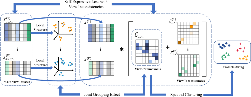
To simultaneously address the above two limitations, in this paper, we propose a novel jointly smoothed multi-view subspace clustering (JSMC) approach. In comparison with previous works, our JSMC approach is able to integrates (i) the cross-view commonness and inconsistencies in subspace representations, (ii) the jointly smoothed regularization via view-consensus grouping effect, and (iii) the low-rank representation into a unified multi-view subspace framework. In particular, to explicitly model the cross-view commonness and inconsistencies, we decompose the subspace representation on each view into a common part and an inconsistent part. In contrast with the conventional practice of extracting consistent parts from multiple views and then constraining these consistent parts to be similar [15] , the commonness is a more strict concept than the consistency. Especially, we aim to discover a common subspace representation across multiple views while simultaneously capturing the view-particularities via the inconsistent parts. To leverage the local structures of multiple views, the view-consensus grouping effect is formulated between the multi-view $K$-nearest neighbor ($K$-NN) graphs and a common subspace representation, which enforces the multi-view smooth regularization on the subspace representation learning. Furthermore, the low-rank constraint is incorporated to enhance the cluster structure in the common subspace representation. With the cross-view consistency and inconsistencies, the view-consensus grouping effect, and the low-rank constraint jointly modeled into a unified objective function, an alternating minimization algorithm is then designed to perform the optimization and learn a robust subspace representation, upon which the spectral clustering can be utilized to achieve the final clustering result. Experiments on eight real-world multi-view datasets demonstrate the superiority of the proposed JSMC approach.

For clarity, the main contributions of this work are summarized as follows:

• We simultaneously and explicitly model the cross-view commonness and inconsistencies to assist the multi-view subspace clustering, which adaptively learns the common subspace representation while capturing view particularities.

• We extend the view-specific grouping effect to view-consensus grouping effect, which together with the inconsistency-aware subspace learning and the low-rank representation learning constitute our unified objective function for robust multi-view subspace clustering.

• A novel multi-view subspace clustering approach termed JSMC is proposed. Extensive experimental results on a variety of multi-view datasets have demonstrated the superior performance of the proposed approach.

The rest of the paper is organized as follows. We review the related work on multi-view clustering in Section 2. The proposed JSMC approach is described in Section 3. Experimental results are reported in Section 4. Finally, the conclusion of the paper is provided in Section 5.

2 Related work

Multi-view clustering aims to utilize the features of multiple views to achieve a unified clustering result. In recent years, many multi-view clustering methods have been designed from different technical perspectives [2, 3, 4, 5, 6, 7, 8, 9, 10, 11, 15, 16, 17, 26, 27, 28, 29, 30, 31, 32, 33, 34]. Some important categories in multi-view clustering include the co-training based methods [2, 3, 4], the multi-kernel based methods [5, 6, 7, 8], the graph learning based methods [9, 10, 11, 12, 32], the deep learning based methods [13, 14], and the subspace learning based methods [15, 16, 17].

The co-training based methods [2, 3, 4, 35] aim to learn a clustering result by minimizing the multi-view disagreement. Kumar et al. [2] proposed a co-training method where each cluster was able to utilize the complementary information learned from other clusters, and applied the co-training method to multi-view spectral clustering. Further, Kumar et al. [3] proposed a multi-view spectral clustering method with co-regularization, which imposed the regularization on the eigenvectors of the graph Laplacians constructed from multiple views. Ye et al. [4] designed a co-regularized kernel $k$-means method that automatically learned the weights of different views for robust clustering.

The multi-kernel based methods [5, 6, 7, 8, 36] express multiple views in terms of multiple kernel matrices and combine the multiple kernels to achieve the final clustering. Tzortzis and Likas [5] proposed a weighted combination scheme for multiple kernels, which iteratively updated the kernel weights and recomputed the cluster labels to optimize the clustering result. Guo et al. [6] proposed a multiple kernel learning method for multi-view spectral clustering, where the kernel matrix learning and the spectral clustering optimization were combined in a unified framework. Zhang et al. [7] designed a multi-view clustering method based on multiple kernel low-rank representation, which combined the co-regularization with the low-rank multiple kernel trick.

The graph learning based methods [9, 10, 11, 12, 32] seek to learn a unified graph by fusing multiple affinity graphs from multiple views. Upon the unified graph, the final clustering can be obtained via some graph partitioning algorithm. Nie et al. [9] took the importance of views into account and developed a self-weighted scheme to fuse the multiple graphs. Zhan et al. [11] learned a consensus graph by minimizing the disagreement between the graphs from different views and incorporating the rank constraint on the Laplacian matrix. Liang et al. [12] considered the consistency and inconsistency in a graph learning framework, and proposed two graph fusion algorithms, termed similarity graph fusion (SGF) and dissimilarity (distance) graph fusion (DGF), respectively.

The deep learning based methods [13, 14] learn the feature representations of multiple views via deep neural networks and typically enforce some consistency constraint on the multi-view representations for obtaining the final clustering. For example, Xie et al. [13] proposed the deep multi-view joint clustering (DMJC) method to learn multi-view feature representations and in the meantime utilize the complementary information among multiple views. Wang et al. [14] designed a generalized deep learning multi-view clustering (GDLMC) method based on nonnegative matrix factorization (NMF).

The subspace learning based methods leverage the self-expressive loss (or reconstruction loss) to discover the low-dimensional subspaces from multiple views for improving representation learning and clustering. Gao et al. [15] presented a multi-view subspace clustering method with the multiple subspace representations constrained to be consistent. Wang et al. [16] incorporated the manifold information of each view by adopting the graph Laplacian regularized low-rank representation in multi-view subspace learning. Zhang et al. [17] learned a shared multi-view latent representation, which is able to depict the data instances more comprehensively than individual views and make the subspace representation more robust.

3 Jointly Smoothed Multi-view Subspace Clustering

In this section, we describe the proposed JSMC approach in detail. Specifically, Section 3.1 presents the incorporation of the view-commonness and view-inconsistencies into the multi-view subspace learning model. Section 3.2 extends the view-specific grouping effect to the view-consensus grouping effect for jointly smoothed regularization. Section 3.3 describes the formulation of the unified objective function, which will be optimized via an alternating minimization algorithm in Section 3.4. Finally, the computational complexity of the proposed JSMC approach is analyzed in Section 3.5.

3.1 Multi-view Inconsistency in Subspace Learning

In this section, we present the formulation of the multi-view subspace learning with cross-view commonness and inconsistencies. In subspace learning, it is generally assumed that the structure of high-dimension data can be represented by a union of low-dimension subspaces. According to the self-expressiveness property [37], a data instance can be represented as a linear combination of other instances. Given a (single-view) dataset $X=\left[\mathbf{x}_{1},\mathbf{x}_{2},\ldots,\mathbf{x}_{n}\right]\in\mathbb{R}^{d\times n}$, where $\mathbf{x}_{i}\in\mathbb{R}^{d}$ is the $i$-th instance, $n$ is the number of instances in the dataset, and $d$ is the dimension, the traditional subspace learning based clustering (or subspace clustering for short) methods typically seek to learn a self-representation matrix by the self-expressiveness property [37], such that

$$X=XZ+A,$$ (1)

where $A\in\mathbb{R}^{n\times n}$ is the error matrix, $Z=\left[\mathbf{z}_{1},\mathbf{z}_{2},\ldots,\mathbf{z}_{n}\right]\in\mathbb{R}^{n\times n}$ is the self-representation matrix, and $\mathbf{z}_{i}$ is a representation vector of data instance $\mathbf{x}_{i}$. The subspace clustering aims to find a better representation by minimizing the self-express error $A$, whose objective function can be formulated as

$$\underset{Z}{\text{min}} \|X-XZ\|_{F}^{2}+\alpha\Omega(Z),$$ (2)

s.t. $$\quad z_{ij}=0,Z^{\top}\mathbf{1}=\mathbf{1},$$

where $z_{ij}$ denotes the $(i,j)$-th entry of $Z$, $\Omega(Z)$ denotes a regularization term on $Z$, and $\alpha\geq 0$ is a hyper-parameter to control the influence of the regularization term. By constraining $z_{ij}=0$, it enforces that each instance $\mathbf{x}_{i}$ can only be represented by other instances. By optimizing the objective (2), the self-representation (i.e., subspace representation) $Z$ can be learned, upon which the symmetrical affinity matrix can be constructed as $W=(|Z|+\left|Z^{\top}\right|)/2$ for the final spectral clustering process [24], where $|\cdot|$ is the absolute operator.

In the multi-view scenarios, the (single-view) subspace clustering formulation can be extended to multiple views by learning a self-representation matrix for each view and then enforcing some consistency constraint on the multiple representations. For most of multi-view subspace clustering algorithms [15, 16, 38, 39], they obtain a unified representation matrix or explore a latent space for all views according to the consensus principle. Given a multi-view dataset $X=\{X^{(1)},X^{(2)},\ldots,X^{(V)}\}\in\mathbb{R}^{d\times n}$, where $X^{(v)}\in\mathbb{R}^{d_{v}\times n}$ is the $v$-th view, $d_{v}$ is the dimension of the $v$-th view. It holds that $d=d_{1}+\cdots+d_{V}$. Then the objective function of the multi-view subspace clustering can be formulated as

$$\min_{Z^{(1)},\cdots,Z^{(V)}}\sum_{v=1}^{V}\left\|X^{(v)}-X^{(v)}Z^{(v)}\right\|_{F}^{2}+\alpha\Omega(Z^{(1)},\cdots,Z^{(V)}),$$ (3)

$$\text{ s.t. }\quad z^{(v)}_{ij}=0,(Z^{(v)})^{\top}\mathbf{1}=\mathbf{1},\text{~{}for~{}}v=1,\cdots,V,$$

where $z^{(v)}_{ij}$ denotes the $(i,j)$-th entry of the self-representation matrix $Z^{(v)}$ of the $v$-th view, and $\Omega(Z^{(1)},\cdots,Z^{(V)})$ denotes the regularization term which typically constrains the consistency of the multiple views. However, the prior works [15, 16, 38, 39] mostly focus on the consistency of the multi-view subspace representations, yet often lack the ability to explicitly capture the inconsistency between different views, which may undermine their ability to make full use of versatile information of multiple views. In light of this, we can decompose the subspace representation $Z^{(v)}$ into a view-consistency matrix $C^{(v)}$ and a view-inconsistency matrix $E^{(v)}$, that is

$$Z^{(v)}=C^{(v)}+E^{(v)}.$$ (4)

Then, the objective function of multi-view subspace clustering can be re-formulated as

$$\underset{C^{(1)},\cdots,C^{(V)},E^{(1)},\cdots,E^{(V)}}{\text{min}} \sum_{v=1}^{V}\|X^{(v)}-X^{(v)}(C^{(v)}+E^{(v)})\|_{F}^{2}$$ (5)

$$+\alpha\Omega_{1}(C^{(1)},\cdots,C^{(V)})+\beta\Omega_{2}(E^{(1)},\cdots,E^{(V)})$$

where $\Omega_{1}(C^{(1)},\cdots,C^{(V)})$ and $\Omega_{2}(E^{(1)},\cdots,E^{(V)})$ are regularization terms on the view-consistency matrices and the view-inconsistency matrices, respectively, and $\alpha\geq 0$ and $\beta\geq 0$ are hyper-parameters.

Further, we aim to extend the concept of view-consistency to a more strict concept of view-commonness. Specifically, the consistency typically requires multiple representations (from multiple views) to be similar, e.g., by enforcing the similarity between the $V$ representations ranging from $C^{(1)}$ to $C^{(V)}$ via the regularization term $\Omega_{1}(\cdot)$ in objective (5), while the concept of commonness goes one step further by extracting a common part from multiple representations. Formally, we can decompose each subspace representation matrix $Z^{(v)}$ into a view-commonness matrix $C$ and a view-inconsistency matrix $E^{(v)}$, that is

$$Z^{(v)}=C+E^{(v)}.$$ (6)

where the view-commonness matrix $C$ is shared by all views and the view-inconsistency matrices $E^{(1)},\cdots,E^{(V)}$ explicitly capture the inconsistencies in multiple views. Note that the inconsistency is a broader concept than noise, which may come from noise or view-specific characteristics. Thereafter, the objective function can be rewritten as

$$\underset{C,E^{(1)},\cdots,E^{(V)}}{\text{min}} \sum_{v=1}^{V}\|X^{(v)}-X^{(v)}(C+E^{(v)})\|_{F}^{2}$$ (7)

$$+\alpha\Omega_{1}(C)+\beta\Omega_{2}(E^{(1)},\cdots,E^{(V)})$$

Notably, the objective (7) can be viewed as a special instance of the objective (5) by additionally constraining that $C^{(1)}=C^{(2)}=\cdots=C^{(V)}$.

3.2 From View-Specific to View-Consensus Grouping Effect

Previous multi-view subspace clustering works [15, 16, 17] often lack the ability to explicitly preserve the locality in the learned subspace representations. To explain this issue, we first discuss it in the single-view scenario. In terms of locality preservation, if two instances $\mathbf{x}_{i}$ and $\mathbf{x}_{j}$ are similar, their subspace representations $\mathbf{z}_{i}$ and $\mathbf{z}_{j}$ should also be close to each other, which is called the grouping effect, also known as the smooth regularization [24]. Formally, the grouping effect is defined in Definition 1.

Definition 1 (Grouping Effect). Given a set of data instances $X=\left[\mathbf{x}_{1},\mathbf{x}_{2},\ldots,\mathbf{x}_{n}\right]\in\mathbb{R}^{d\times n}$, a self-representation matrix $Z=\left[\mathbf{z}_{1},\mathbf{z}_{2},\ldots,\mathbf{z}_{n}\right]\in\mathbb{R}^{n\times n}$ has the grouping effect if $\left\|\mathbf{x}_{i}-\mathbf{x}_{j}\right\|_{2}\rightarrow 0\Rightarrow\left\|\mathbf{z}_{i}-\mathbf{z}_{j}\right\|_{2}\rightarrow 0,\forall i\neq j$.

The smooth regularization (via grouping effect) has shown its advantage in locality preserving for single-view clustering [24]. Recently Chen et al. [25] incorporated the grouping effect into the multi-view subspace clustering in a view-specific manner, which enforces the grouping effect on each view separately but still cannot exploit the grouping effect of multiple views in a jointly smoothed formulation.

From the view-specific perspective, for the $v$-th view, if the subspace representation $Z^{(v)}$ is decomposed into a view-consistency representation $C^{(v)}$ and a view-inconsistency representation $E^{(v)}$ (as shown in Eq. (4)), then we can enforce the view-specific grouping effect by considering the affinity (or similarity) of two instances $\mathbf{x}^{(v)}_{i}$ and $\mathbf{x}^{(v)}_{j}$ and their view-consistency representations $\mathbf{c}^{(v)}_{i}$ and $\mathbf{c}^{(v)}_{j}$. More specifically, for the $v$-th view, if $\mathbf{x}^{(v)}_{i}$ and $\mathbf{x}^{(v)}_{j}$ are similar, then $\mathbf{c}^{(v)}_{i}$ and $\mathbf{c}^{(v)}_{j}$ should also be close to each other, which can be achieved by optimizing the following objective:

$$\underset{C^{(v)}}{\text{min}}\frac{1}{2}\sum_{i=1}^{n}\sum_{j=1}^{n}w_{ij}^{(v)}\left\|\mathbf{c}_{i}^{(v)}-\mathbf{c}_{j}^{(v)}\right\|_{2}^{2},$$ (8)

where $W^{(v)}$ denotes the affinity matrix (or similarity matrix) with $w_{ij}^{(v)}$ being its $(i,j)$-th entry. In general, the affinity matrix $W^{(v)}$ can be defined by constructing a fully-connected graph, an $\varepsilon$-neighbor graph, or a $K$-nearest neighbor ($K$-NN) graph. In this work, the $K$-NN graph is adopted to preserve the local structure of the data. Let $L^{(v)}=D^{(v)}-W^{(v)}$ be the Laplacian matrix of $W^{(v)}$, where $D^{(v)}$ is the degree matrix with its $(i,j)$-th entry being $d_{ii}^{(v)}=\sum_{j}w_{ij}^{(v)}$. Then the objective (8) can be rewritten as

$$\underset{C^{(v)}}{\text{min}}\operatorname{Tr}\left(C^{(v)}L^{(v)}(C^{(v)})^{\top}\right).$$ (9)

To extend from view-consistency to view-commonness (as discussed in Section 3.1), we decompose the subspace representation $Z^{(v)}$ into a view-commonness matrix $C$ and a view-inconsistency matrix $E^{(v)}$. To jointly enforce the grouping effect, we expect that the local structures in different views can jointly influence the learning of the common representation matrix $C$, which gives rise to the following objective:

$$\underset{C}{\text{min}}\frac{1}{2}\sum_{v=1}^{V}\sum_{i=1}^{n}\sum_{j=1}^{n}w^{(v)}_{ij}\|\mathbf{c}_{i}-\mathbf{c}_{j}\|_{2}^{2},$$ (10)

where $\mathbf{c}_{i}$ and $\mathbf{c}_{j}$ denote the common representations of the $i$-th and $j$-th instances, respectively. Further, the objective (10) can be rewritten as

$$\underset{C}{\text{min}}\sum_{v=1}^{V}\operatorname{Tr}(CL^{(v)}C^{\top}).$$ (11)

Different from the conventional view-specific grouping effect [25], through the objective 10, we enforce the grouping effect in a view-consensus manner, which collectively explores the local structures of multiple views to assist the learning of the multi-view common representation.

3.3 Overall Objective Function

With the cross-view consistency and inconsistency captured in objective (7) and the view-consensus grouping effect exploited in objective (11), in this section, we further specify the regularization terms on the view-commonness and view-inconsistency matrices, and present the overall objective function of the proposed approach.

For the view-commonness matrix, i.e., the common representation matrix $C$, we take advantage of the low rank constraint via the nuclear norm, which reduces the redundancy of the matrix and enhances the cluster structure [40]. That is

$$\underset{C}{\text{min}}\|C\|_{*}.$$ (12)

For the view-inconsistency matrices $E^{(1)},\cdots,E^{(V)}$, the Frobenius norm is utilized to regularize them. That is

$$\underset{E^{(1)},\ldots,E^{(V)}}{\text{min}}\sum_{v=1}^{V}{\|E^{(v)}\|_{F}^{2}}.$$ (13)

From objectives (7), (11), (12), and (13), the overall objective function can be formulated as follows:

$$\underset{C,E^{(1)},\ldots,E^{(V)}}{\text{min}} \mathcal{O}\left(C,E^{(1)},\ldots,E^{(V)}\right)=$$ (14)

$$\underbrace{\sum_{v=1}^{V}\|X^{(v)}-X^{(v)}(C+E^{(v)})\|_{F}^{2}}_{\text{Inconsistency-Aware Self-Expressive Loss}}+\underbrace{\alpha\sum_{v=1}^{V}\operatorname{Tr}(CL^{(v)}C^{\top})}_{\text{Jointly Smoothed Representation}}$$

$$+\underbrace{\beta\sum_{v=1}^{V}{\|E^{(v)}\|_{F}^{2}}}_{\text{View-Inconsistency Regularization}}+\underbrace{\lambda\|C\|_{*}}_{\text{Low-Rank Regularization}}$$

With this objective function, the cross-view consistency and inconsistency, the view-consensus grouping effect, and the low rank representation are simultaneously leveraged. With the common representation $C$ learned, the spectral clustering can then be utilized to obtain the final clustering. In the following section, we will present the optimization of the unified objective function.

3.4 Optimization

In this section, we optimize the objective function (14) by using an alternating minimizing algorithm. Before solving this problem, to make the problem separable, we introduce an auxiliary variable $S$ for the common representation matrix $C$ such that $S=C$. Thus, the objective (14) can be rewritten as follows:

$$\underset{S,C,E^{(1)},\ldots,E^{(V)}}{\text{min}} \mathcal{O}\left(S,C,E^{(1)},\ldots,E^{(V)}\right)=$$ (15)

$$\sum_{v=1}^{V}\|X^{(v)}-X^{(v)}(S+E^{(v)})\|_{F}^{2}+\alpha\sum_{v=1}^{V}\operatorname{Tr}(SL^{(v)}S^{\top})$$

$$+\beta\sum_{v=1}^{V}{\|E^{(v)}\|_{F}^{2}}+\lambda\|C\|_{*}$$

$$\text{ s.t. }\quad S=C$$

Then we have the corresponding augmented Lagrangian function:

$$\underset{S,C,E^{(1)},\ldots,E^{(V)}}{\text{min}} \mathcal{L}\left(S,C,E^{(1)},\ldots,E^{(V)}\right)=$$ (16)

$$\sum_{v=1}^{V}\|X^{(v)}-X^{(v)}(S+E^{(v)})\|_{F}^{2}+\alpha\sum_{v=1}^{V}\operatorname{Tr}(SL^{(v)}S^{\top})$$

$$+\beta\sum_{v=1}^{V}{\|E^{(v)}\|_{F}^{2}}+\lambda\|C\|_{*}+\frac{\mu}{2}\|S-C+\frac{Y}{\mu}\|_{F}^{2}$$

where $\mu>0$ is the penalty parameter, and $Y$ is the Lagrangian multiplier. Next, each variable can be iterative updated with other variables fixed [41].

3.4.1 $S$-Subproblem

With $E^{(1)},\ldots,E^{(V)}$ and $C$ fixed, the variable $S$ is updated. Specifically, the objective (16) can be rewritten as follows:

$$\underset{S}{\text{min}}\mathcal{L}\left(S\right) =\sum_{v=1}^{V}\|X^{(v)}-X^{(v)}(S+E^{(v)})\|_{F}^{2}$$ (17)

$$+\alpha\sum_{v=1}^{V}\operatorname{Tr}(SL^{(v)}S^{\top})+\frac{\mu}{2}\|S-C+\frac{Y}{\mu}\|_{F}^{2}$$

Then we obtain its partial derivative w.r.t. $S$, that is

$$\frac{\partial\mathcal{L}(\mathrm{S})}{\partial S} =\sum_{v=1}^{V}2X^{(v)^{\top}}X^{(v)}\left(-I+S+E^{(v)}\right)$$ (18)

$$+2\alpha\sum_{v=1}^{V}SL^{(v)}+\frac{\mu}{2}\left(2S-2C+\frac{2}{\mu}Y\right),$$

where $I$ is an identity matrix. By setting $\frac{\partial\mathcal{L}(\mathrm{S})}{\partial S}=0$, we have

$$\left(2\sum_{v=1}^{V}X^{(v)^{\top}}X^{(v)}+\mu I\right)S+S*2\alpha\sum_{v=1}^{V}L^{(v)}$$ (19)

$$=\sum_{v=1}^{V}\left[2X^{(v)^{\top}}X^{(v)}\left(I-E^{(v)}\right)\right]+\mu C-Y$$

The problem in Eq. (19) is a standard Sylvester equation. Therefore, the Bartels-Stewart algorithm [42] can be utilized to solve this problem.

3.4.2 $C$-Subproblem

With $E^{(1)},\ldots,E^{(V)}$ and $S$ fixed, the variable $C$ is updated. The objective (16) w.r.t. the common representation matrix $C$ can be rewritten as follows:

$$\underset{C}{\text{min}}\quad\mathcal{L}\left(C\right)=\lambda\|C\|_{*}+\frac{\mu}{2}\|S-C+\frac{Y}{\mu}\|_{F}^{2}$$ (20)

By solving this problem via the singular value thresholding (SVT) operator [43], we have

$$C=U_{C}\delta_{\frac{\lambda}{\mu}}(\Sigma_{C})V_{C}^{\top},$$ (21)

where $U_{C}\Sigma_{C}V_{C}^{\top}$ denotes the singular value decomposition (SVD) of $S+\frac{Y}{\mu}$, and $\delta_{\frac{\lambda}{\mu}}(\cdot)$ denotes the shrinkage operator, which can be defined as

$$\delta_{\frac{\lambda}{\mu}}(\Sigma_{C})=\max\left(0,\Sigma_{C}-\frac{\lambda}{\mu}\right)+\min\left(0,\Sigma_{C}+\frac{\lambda}{\mu}\right)$$ (22)

3.4.3 $E^{(v)}$-Subproblem

With $C$ and $S$ fixed, the variables $E^{(1)},\ldots,E^{(V)}$ are updated. The objective (16) w.r.t. the view-inconsistency matrices can be rewritten as

$$\underset{E^{(1)},\ldots,E^{(V)}}{\text{min}}\mathcal{L}\left(E^{(1)},\ldots,E^{(V)}\right)=$$ (23)

$$\quad\sum_{v=1}^{V}\|X^{(v)}-X^{(v)}(S+E^{(v)})\|_{F}^{2}+\beta\sum_{v=1}^{V}{\|E^{(v)}\|_{F}^{2}}$$

In particular, for each view $v$, its view-inconsistency matrix $E^{(v)}$ can be updated respectively. Then the objective (LABEL:eq:Eupdate) can be reformulated as follows:

$$\underset{E^{(v)}}{\text{min}}\mathcal{L}\left(E^{(v)}\right)=\|X^{(v)}-X^{(v)}(S+E^{(v)})\|_{F}^{2}+\beta{\|E^{(v)}\|_{F}^{2}}$$ (24)

By setting the derivative of the above objective function to $0$, $E^{(v)}$ can be updated as follows:

$$E^{(v)}=\left(X^{(v)^{\top}}X^{(v)}+\beta I\right)^{-1}\left[X^{(v)^{\top}}X^{(v)}(I-S)\right]$$ (25)

3.4.4 Update Multiplier

In each iteration, after updating other variables, the multiplier $Y$ can be updated as

$$Y=Y+\mu(S-C)$$ (26)

By iteratively updating all variables until convergence or reaching the maximum number of iterations, a unified view-commonness matrix, i.e., the common representation matrix $C$, can be obtained, based on which the affinity matrix can be constructed and the final clustering result can be achieved via the spectral clustering. For clarity, we summarize the overall algorithm of our JSMC approach in Algorithm 1.

Algorithm 1 Jointly Smoothed Multi-view subspace Clustering (JSMC).

1:  Input: Multi-view dataset $X=\{X^{(1)},X^{(2)},\ldots,X^{(V)}\}$, the number of clusters $n_{c}$, the parameters $\alpha$, $\beta$ and $\lambda$.

2:  Initialization: $C$ is initialized as the average $K$-NN graph for all the views, $S=0$, $E^{(v)}=0$, $Y=0$.

3:  repeat

4:     Update variable $S$ by solving Eq. (19).

5:     Update view-commonness matrix $C$ by solving Eq. (21).

6:     for $v=1,\ldots,V$ do

7:        Update view-inconsistency matrix $E^{(v)}$ by solving Eq. (25).

8:     end for

9:     Update the multiplier $Y$ by solving Eq. (26).

10:  until Convergence or reaching the maximum number of iterations

11:  Construct the affinity matrix $W=(|C|+\left|C^{\top}\right|)/2$.

12:  Partition $W$ into $n_{c}$ clusters via the spectral clustering .

13:  Output: The clustering result with $n_{c}$ clusters.

3.5 Computational Complexity

In this section, we analyze the computational complexity of the proposed JSMC approach (as described in Algorithm 1).

In the initialization of $C$, the construction of the $K$-NN graphs on $V$ views takes $O(n^{2}V)$ time. In each iteration of JSMC, the first step is to update the auxiliary variable $S$ by solving the standard Sylvester equation via the Bartels-Stewart algorithm, whose time complexity is $O(n^{3})$. In the second step, the main computational cost for updating the common representation matrix $C$ comes from the SVD operation, which takes $O(n^{3})$ time. Then, updating $E^{(v)}$ with the inverse operation in the third step takes $O(n^{3}V)$ time. Therefore, the time complexity of one iteration is $O(n^{3}V)$. After the optimization, the final clustering is obtained by the spectral clustering, which involves the SVD and takes $O(n^{3})$ time. Thus the time complexity of the proposed approach is $O(n^{3}Vt)$, where $t$ is the number of iterations. The space complexity of the proposed approach is $O(n^{2})$ due to the storage of several $n\times n$ matrices.

3.6 Convexity Analysis

In this section, we analyze the convexity of our objective function. For the objective function (14), an auxiliary variable $S$ is introduced for the common representation matrix $C$ such that $S=C$. For the $S$-subproblem, the function w.r.t. the auxiliary variable $S$ (in Eq. (19)) is a standard Sylvester equation, with which we can directly obtain the unique solution of $S$. The Hessian matrix of Eq. (19) is

$$\frac{\partial^{2}\mathcal{L}}{\partial S\partial S^{\top}}=2\sum_{v=1}^{V}\,(X^{(v)^{\top}}X^{(v)}+\alpha L^{(v)})+\mu I$$ (27)

where $I$ is an identity matrix. According to Theorem 1, for any non-zero vector $f$, we have

$$f^{\top}\left(2\sum_{v=1}^{V}\,X^{(v)^{\top}}X^{(v)}+\mu I\right)f =2f^{\top}\left(\sum_{v=1}^{V}\,X^{(v)^{\top}}X^{(v)}\right)f+\mu f^{\top}If$$ (28)

$$=2\sum_{v=1}^{V}\|X^{(v)}f\|_{F}^{2}+\mu\|f\|_{2}^{2}\geq 0$$

With the Laplacian matrix $L^{(v)}$ being positive semi-definite, the Hessian matrix of Eq. (19) is also a positive semi-definite matrix. Thus, the subproblem w.r.t. $S$ in Eq. (19) is convex [44].

Theorem 1.

Given a real symmetric matrix $A\in\mathbb{R}^{n\times n}$, $A$ is a positive semi-definite matrix if for any non-zero vector $f\in\mathbb{R}^{n}$, $f^{\top}Af\geq 0$ holds.

For the $C$-subproblem, we update the view-commonness matrix $C$ while fixing the other variables. The objective function (LABEL:eq:originalC) w.r.t. $C$ is convex according to [43].

For the $E^{(v)}$-subproblem, we update the view-inconsistency matrix $E^{(v)}$ in objective (LABEL:eq:Eupdate) while fixing the other variables. Note that each $E^{(v)}$ can be updated respectively. For each $E^{(v)}$, the Hessian matrix can be obtained as

$$\frac{\partial^{2}\mathcal{L}}{\partial E^{(v)}\partial E^{(v)^{\top}}}=2X^{(v)^{\top}}X^{(v)}+2\beta I$$ (29)

For any non-zero vector $f$, we have

$$f^{\top}\left(2X^{(v)^{\top}}X^{(v)}+2\beta I\right)f =2f^{\top}X^{(v)^{\top}}X^{(v)}f+2\beta f^{\top}If$$ (30)

$$=2\|X^{(v)}f\|_{F}^{2}+2\beta\|f\|_{2}^{2}\geq 0$$

Therefore, the Hessian matrix of each $E^{(v)}$ is a positive semi-definite matrix. Thus the subproblem w.r.t. $E^{(v)}$ is convex [44].

4 Experiment

In this section, we conduct extensive experiments on a variety of real-world datasets to evaluate the proposed JSMC approach against the state-of-the-art multi-view clustering approaches. The details of datasets and evaluation measures are introduced in Section 4.1. The baseline approaches are presented in Section 4.2. The performance comparison of the proposed approach against other multi-view clustering approaches is reported in Section 4.3. The sensitivity of the parameters is evaluated in Section 4.5. Finally, the convergence analysis and ablation study are provided in Sections 4.6 and 4.7, respectively.

4.1 Datasets ana Evaluation Measures

In our experiments, eight real-world datasets are used, including 3Sources, Notting-Hill, ORL, WebKB-Texas, Yale, Reuters, COIL-20, and Caltech-7, which will be introduced as follows.

• 3Sources. This dataset is a multi-view text dataset with $948$ news articles, which includes three online news sources, i.e., BBC, Reuters, and Guardian [45]. In the 3Sources dataset, each news article belongs to one of the six categories, i.e., business, politics, health, entertainment, sport, and technology. In the experiments, only data instances that are complete in all views are selected. The dimensions of the three views, i.e., BBC, Reuters and Guardian, are $3068$, $3631$, and $3560$, respectively.

• Notting-Hill. This dataset is a video image dataset from the movie “Notting Hill” [46]. In $76$ video clips from the movie, $4660$ face images of $5$ characters are collected, where each face image has a pixel-size of $120\times 150$. In the experiments, $550$ face images are included, which are associated with three views, namely, Intensity (2000-D), Gabor (6750-D), and LBP (3304-D).

• ORL. This dataset consists of $400$ face images from $40$ persons [47]. Each face image is taken with different facial expressions, facial details, and lighting conditions. In the ORL dataset, three views are included, namely, Intensity (4096-D), Gabor (6750-D), and LBP (3304-D).

• WebKB-Texas. This dataset is a collection of 187 documents from the homepage of the Computer Science Department of the University of Texas [48]. These documents are grouped into the following tags: student, project, course, staff and faculty. Each document is associated with two views, i.e., citation and content, whose dimensions are $187$ and $1703$, respectively.

• Yale. This dataset consists of $165$ face images from $15$ persons [49], each of which has $11$ gray-scale images with different facial expressions, such as with glasses, without glasses, center-light, left-light, right-light, normal, happy, sad, sleepy, surprised, and wink. In this dataset, three views are included, namely, Intensity (4096-D), Gabor (6750-D), and LBP (3304-D).

• Reuters. This dataset consists of $1200$ documents [17], which are divided into six categories, namely, E$21$, CCAT, M$11$, GCAT, C$15$, and ECAT. Each document in the Reuters dataset is associated with five views, corresponding to five different languages, i.e., English (2000-D), French (2000-D), German (2000-D), Italian (2000-D), and Spanish (2000-D).

• COIL-20. This dataset is a collection of gray-scale images of $20$ objects [50], which are taken from different angles with $72$ poses each. In the COIL-20 dataset, there are three different views, i.e., Intensity (1024-D), LBP (3304-D), and Gabor (6750-D).

• Caltech-7. This dataset is a subset of the Caltech-101 dataset [51], which has images of objects belonging to $101$ classes. Each image is about $200\times 300$ pixels in this subset. In the experiments, we select images from $7$ classes, including Faces, Garfield, Stop-Sign, Snoopy, Windsor-Chair, Motorbikes, and Dollar Bill. Three views are extracted for each image, namely, GIST (512-D), HOG (1984-D), and LBP (928-D).

To evaluate the performances of different multi-view clustering algorithms, four widely-used evaluation measures are adopted, namely, normalized mutual information (NMI) [52], adjusted Rand index (ARI) [53], accuracy (ACC) [54], and purity (PUR) [55].

4.2 Baseline Methods and Experimental Settings

In the experiments, we compare the proposed JSMC method against the spectral clustering method as well as seven multi-view clustering methods, which will be described as follows.

• SC_best [56]. Spectral clustering (SC) is a classical (single-view) clustering method. In the experiments, we conduct spectral clustering on each single view, and report its best single-view performance.

• MVSpec [5]. Multi-view spectral clustering (MVSpec) represents each view with a kernel matrix and captures the importance of different views via a weighted combination of kernels for multi-view clustering.

• RMSC [57]. Robust multi-view spectral clustering (RMSC) constructs a unified probability matrix from multiple probability matrices with the low-rank constraint. Then the unified matrix is partitioned for obtaining the final clustering.

• MVSC [58]. Multi-view spectral clustering (MVSC) first constructs a bipartite graph between the data instances and a set of anchors on each view, and then fuses the multiple bipartite graphs from different views into a unified bipartite graph, upon which the graph partitioning is performed to obtain the clustering result.

• MVGL [59]. Multi-view graph learning (MVGL) fuses multiple affinity graphs from multiple views into a unified graph with the rank constraint, and obtains the clustering result by partitioning the unified graph.

• BMVC [55]. Binary multi-view clustering (BMVC) solves the multi-view clustering problem by binary representation, which simultaneously optimizes the binary learning and the clustering for the multi-view dataset.

• SMVSC [60]. Scalable multi-view subspace clustering (SMVSC) jointly optimizes the anchor learning and the unified graph construction, where the latent structures of data can be expressed by the subspace representation via a set of unified anchors.

• FPMVS-CAG [61]. Fast parameter-free multi-view subspace clustering with consensus anchor guidance (FPMVS-CAG) combines the anchor selection and the graph construction into a parameter-free manner, and learns an anchor-based subspace representation for the final clustering.

In the experiments, we adopt the grid search scheme to find best parameters on each dataset. For the proposed method and all the baseline methods, each parameter is searched in the range of $\{10^{-5},10^{-4},\cdots,10^{5}\}$, unless a specific range of the parameter is suggested in the corresponding paper.

Table 1: Average performances (w.r.t. NMI(%)) of different methods. The best score in each row is highlighted in bold.

Method	SCbest	MVSpec	RMSC	MVSC	MVGL	BMVC	SMVSC	FPMVS-CAG	JSMC
3Sources	38.69±0.00	6.61±0.00	58.56±3.50	66.48±3.46	8.07±0.00	58.69±0.00	8.92±0.00	6.59±0.00	69.52±0.00
Notting-Hill	72.62±0.00	2.22±0.00	71.29±3.68	77.09±8.11	85.51±0.00	4.14±0.00	82.49±0.00	71.35±0.00	96.92±0.00
ORL	89.12±0.00	39.42±0.00	84.79±1.43	84.69±2.06	82.96±0.00	39.29±0.00	75.26±0.00	74.30±0.00	91.46±0.00
WebKB-Texas	29.36±0.00	10.15±0.00	26.01±5.69	1.98±0.25	6.55±0.00	24.73±0.00	21.42±0.00	22.76±0.00	38.04±0.00
Yale	64.94±0.00	25.41±0.00	66.36±2.76	64.10±3.25	67.15±0.00	27.57±0.00	61.68±0.00	49.76±0.00	76.38±0.00
Reuters	23.67±0.00	1.85±0.00	33.01±1.68	1.26±0.46	4.31±0.00	22.46±0.00	18.87±0.00	20.64±0.00	25.96±0.00
COIL-20	80.80±0.00	24.36±0.00	80.42±1.75	75.68±4.33	91.80±0.00	50.69±0.00	73.48±0.00	74.63±0.00	92.98±0.00
Caltech-7	38.26±0.00	10.79±0.00	42.11±1.33	54.46±11.37	55.98±0.00	47.29±0.00	47.79±0.00	47.32±0.00	63.20±0.00
Avg. score	54.68	15.10	57.82	53.22	50.29	34.36	48.74	45.92	69.31
Avg. rank	4.00	8.38	4.00	4.88	4.25	6.13	5.50	6.13	1.13

Table 2: Average performances (w.r.t. ARI(%)) of different methods. The best score in each row is highlighted in bold.

Method	SCbest	MVSpec	RMSC	MVSC	MVGL	BMVC	SMVSC	FPMVS-CAG	JSMC
3Sources	20.81±0.00	0.85±0.00	48.87±3.39	58.38±4.37	-0.72±0.00	54.32±0.00	4.00±0.00	1.01±0.00	65.17±0.00
Notting-Hill	73.93±0.00	1.09±0.00	69.26±5.15	74.52±9.88	81.74±0.00	2.66±0.00	83.95±0.00	62.25±0.00	97.69±0.00
ORL	69.75±0.00	1.98±0.00	61.42±3.28	56.95±6.96	38.79±0.00	0.61±0.00	42.39±0.00	39.99±0.00	77.79±0.00
WebKB-Texas	23.91±0.00	-4.64±0.00	18.51±5.09	0.19±0.35	2.48±0.00	25.18±0.00	29.01±0.00	29.81±0.00	32.26±0.00
Yale	45.06±0.00	0.26±0.00	45.64±3.98	40.15±5.28	41.53±0.00	1.77±0.00	37.56±0.00	25.30±0.00	57.58±0.00
Reuters	17.19±0.00	0.24±0.00	26.15±1.15	0.05±0.03	0.27±0.00	17.00±0.00	11.85±0.00	16.91±0.00	20.48±0.00
COIL-20	66.79±0.00	4.48±0.00	66.14±3.19	51.95±8.71	78.21±0.00	27.83±0.00	51.14±0.00	53.21±0.00	81.28±0.00
Caltech-7	30.55±0.00	-1.73±0.00	32.05±2.62	47.92±14.14	41.99±0.00	36.34±0.00	38.21±0.00	41.34±0.00	60.10±0.00
Avg. score	43.50	0.32	46.00	41.26	35.54	20.71	37.26	33.73	61.54
Avg. rank	4.25	8.63	4.13	4.88	5.13	6.13	5.00	5.38	1.13

4.3 Performance Comparison and Analysis

In this section, we compare our proposed JSMC method with other multi-view clustering methods. Specifically, we run each of the test methods twenty times, and report their average performances w.r.t. to NMI, ARI, ACC, and PUR in Tables 1, 2, 3, and 4, respectively.

As shown in Table 1, our JSMC method achieves the best performance w.r.t. NMI on seven out of eight benchmark datasets. Though the RMSC method obtains a higher NMI score than JSMC on the Reuters dataset, yet our JSMC method yield higher or significantly higher NMI scores than RMSC on all the other seven datasets. Especially, on the Notting-Hill datasets, our JSMC method achieves an NMI(%) score of 96.92, whereas the second best method (i.e., MVGL) only achieves an NMI(%) score of 85.51. Further, we also report the average score and average rank (across the eight benchmark datasets) for the proposed method and the baseline methods. In terms of average score, our JSMC method achieves an average NMI(%) score (across eight datasets) of 69.31, which is significantly higher than the second best average NMI(%) score of 57.82 (achieved by RMSC). In terms of average rank, our JSMC method achieves an average rank of 1.13, whereas the second best method only achieves an average rank of 4.00.

Table 3: Average performances (w.r.t. ACC(%)) of different methods. The best score in each row is highlighted in bold.

Method	SCbest	MVSpec	RMSC	MVSC	MVGL	BMVC	SMVSC	FPMVS-CAG	JSMC
3Sources	48.52±0.00	25.44±0.00	62.54±4.31	75.86±4.58	35.50±0.00	65.68±0.00	31.36±0.00	26.04±0.00	77.51±0.00
Notting-Hill	86.55±0.00	26.36±0.00	79.41±3.22	81.20±5.86	84.36±0.00	27.27±0.00	91.45±0.00	70.55±0.00	98.91±0.00
ORL	77.25±0.00	19.50±0.00	70.23±2.73	72.36±3.81	72.00±0.00	16.75±0.00	56.25±0.00	56.00±0.00	82.00±0.00
WebKB-Texas	57.75±0.00	32.09±0.00	48.64±4.80	55.13±0.30	51.87±0.00	56.68±0.00	56.68±0.00	57.75±0.00	59.89±0.00
Yale	63.64±0.00	21.82±0.00	61.21±4.24	59.03±4.26	64.85±0.00	22.42±0.00	56.97±0.00	44.24±0.00	73.33±0.00
Reuters	42.00±0.00	20.75±0.00	52.60±2.60	17.59±0.43	18.92±0.00	45.00±0.00	38.08±0.00	44.33±0.00	46.75±0.00
COIL-20	72.36±0.00	15.76±0.00	70.84±4.09	61.66±6.58	81.39±0.02	40.63±0.00	60.56±0.00	63.75±0.00	83.96±0.00
Caltech-7	46.40±0.00	38.87±0.00	40.39±2.82	63.68±6.14	66.28±0.00	47.15±0.00	46.68±0.00	54.55±0.00	70.90±0.00
Avg.score	61.81	25.07	60.73	60.81	59.40	40.20	54.75	52.15	74.16
Avg. rank	3.75	8.63	5.00	4.75	4.25	5.88	5.50	5.50	1.13

Table 4: Average performances (w.r.t. PUR(%)) of different methods. The best score in each row is highlighted in bold.

Method	SCbest	MVSpec	RMSC	MVSC	MVGL	BMVC	SMVSC	FPMVS-CAG	JSMC
3Sources	59.17±0.00	39.64±0.00	76.33±3.60	80.89±3.26	40.24±0.00	73.37±0.00	44.38±0.00	42.60±0.00	82.25±0.00
Notting-Hill	86.55±0.00	32.36±0.00	82.23±1.94	83.55±6.19	87.09±0.00	35.64±0.00	91.45±0.00	82.73±0.00	98.91±0.00
ORL	80.00±0.00	21.25±0.00	74.31±2.22	77.05±2.47	77.75±0.00	18.00±0.00	60.25±0.00	60.00±0.00	84.50±0.00
WebKB-Texas	69.52±0.00	55.08±0.00	68.80±4.35	56.10±0.16	57.22±0.00	68.98±0.00	67.91±0.00	65.78±0.00	70.05±0.00
Yale	64.24±0.00	22.42±0.00	62.36±4.02	60.33±3.59	64.85±0.00	24.24±0.00	56.97±0.00	46.67±0.00	73.94±0.00
Reuters	43.75±0.00	20.83±0.00	54.40±1.81	17.90±0.45	20.83±0.00	45.33±0.00	40.50±0.00	46.83±0.00	48.58±0.00
COIL-20	74.72±0.00	23.19±0.00	72.51±3.11	64.69±5.64	86.25±0.00	40.76±0.00	61.67±0.00	65.42±0.00	88.68±0.00
Caltech-7	82.29±0.00	55.16±0.00	84.13±1.35	82.91±7.85	85.35±0.00	84.94±0.00	87.31±0.00	84.74±0.00	92.06±0.00
Avg.score	70.03	33.74	71.88	65.43	64.95	48.91	63.81	61.85	79.87
Avg. rank	4.00	8.63	4.25	5.75	4.38	6.00	5.00	5.75	1.13

Figure 2: Running time of different algorithms on the eight datasets.

Similar advantages of the proposed JSMC method can also be observed in Tables 2, 3, and 4, corresponding to the ARI, ACC, and PUR scores, respectively. In terms of ARI(%), our JSMC method achieves an average score of 61.54 and an average rank of 1.13, whereas the second best method achieves an average score of 46.00 and an average rank of 4.13. In terms of ACC(%), our JSMC method achieves an average score of 74.16 and an average rank of 1.13, whereas the second best method achieves an average score of 61.81 and an average rank of 3.75. In terms of PUR(%), our JSMC method achieves an average score of 79.87 and an average rank of 1.13, whereas the second best method achieves an average score of 71.88 and an average rank of 3.75. To summarize, the experimental results in Tables 1, 2, 3, and 4 have shown the accuracy and robustness of the proposed JSMC method over the other multi-view clustering methods.

4.4 Analysis of Time and Memory Costs

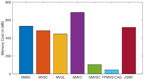
In this section, we compare the time and memory costs of different methods in Figs. 2 and 3, respectively. In terms of time cost, as shown in Fig. 2, our JSMC method is faster than FPMVS-CAG on the ORL, WebKB-Texas, and Yale datasets, and slower than FPMVS-CAG on the other datasets. In terms of the memory cost, we compare the memory costs of different methods on the Caltech-7 dataset. As shown in Fig. 3, the two bipartite graph based methods (i.e., SMVSC and FPMVS) consume less memory than the other methods on the Caltech-7 dataset, while the memory cost of our JSMC method is comparable to RMSC, MVSC, MVGL, and BMVC. To summarize, as can be observed in Tables Tables 1, 2, 3, and 4 and Figs. 2 and 3, our JSMC method requires comparable computational costs to some general baseline methods, while producing highly-competitive (or advantageous) clustering performance on the benchmark datasets.

Figure 3: Memory costs of different algorithms on the Caltech-7 dataset.

4.5 Parameter Analysis

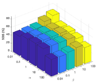
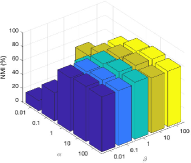
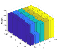
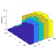
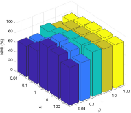
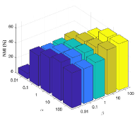
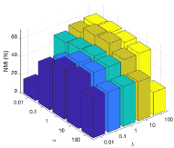
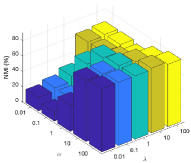
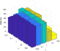
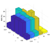
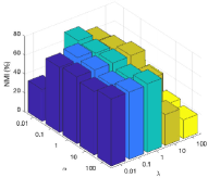
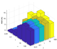
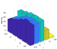
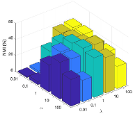
In this section, we evaluate the performance (w.r.t. NMI(%)) of the proposed JSMC method with varying parameter settings on the benchmark datasets. Specifically, we first evaluate the performance of JSMC with varying parameters $\alpha$ and $\beta$, and illustrate the performance results in Fig. 4. Then we evaluate the performance of JSMC with varying parameters $\alpha$ and $\lambda$, and illustrate the performance results in Fig. 5. As shown in Figs. 4, and 5, the proposed JSMC method has shown relative consistent performance with varying parameter settings. Especially, setting the three parameters, i.e., $\alpha$, $\beta$, and $\lambda$, to moderate values can generally lead to favorable clustering results on the benchmark datasets.

(a) 3Sources

(b) Notting-Hill

(c) ORL

(d) WebKB-Texas

(e) Yale

(f) Reuters

(g) COIL-20

(h) Caltech-7

Figure 4: Performance of the proposed JSMC method with varying parameters $\alpha$ and $\beta$ on the benchmark datasets.

(a) 3Sources

(b) Notting-Hill

(c) ORL

(d) WebKB-Texas

(e) Yale

(f) Reuters

(g) COIL-20

(h) Caltech-7

Figure 5: Performance of the proposed JSMC method with varying parameters $\alpha$ and $\lambda$ on the benchmark datasets.

(a) 3Sources

(b) Notting-Hill

(c) ORL

(d) WebKB-Texas

(e) Yale

(f) Reuters

(g) COIL-20

(h) Caltech-7

Figure 6: Convergence of the objective function (14) with increasing iterations on the eight benchmark datasets.

4.6 Convergence Analysis

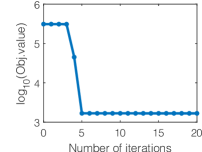
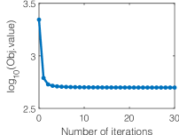
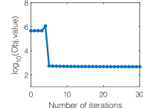
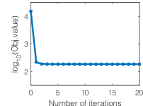
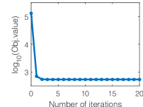
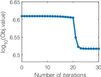
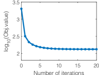
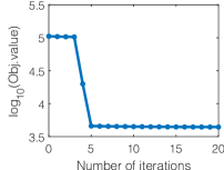
In this section, we analyze the convergence of the proposed JSMC method on the benchmark datasets. In JSMC, the objective function (14) is formulated with the cross-view consistency and inconsistency, the view-consensus grouping effect, and the low-rank representation simutaneously considered, which is then optimized by an alternating optimization algorithm. As shown in Fig. 6, the convergence of the objective function (14) is generally reached within thirty iterations, which indicates a fast convergence speed of the proposed method on a variety of datasets.

4.7 Ablation Study

In this section, the ablation study is conducted to test the influences of different terms (or components) in our objective function (14). Specifically, the influences of three terms, i.e., the inconsistency term, the smoothness term (via the grouping effect), and the low-rank regularization term, are evluated, with the evaluation results w.r.t. NMI, ARI, ACC, and PUR reported in Tables 5, 6, 7, 8, respectively. In each of these four tables, the first column corresponds to the results of JSMC with all the three terms (or components). The second, third, and fourth columns correspond to the results with one component removed. And the fifth, sixth, and seventh columns correspond to the results with two components removed.

As shown in Tables 5, the average NMI(%) score across eight datasets is 69.31. When removing each of the three components, the average NMI(%) scores decrease to 61.75, 59.78, and 65.24, respectively, which demonstrate the advantageous contributions of the three components. Moreover, when removing two of the three components and only preserving one of them, the average NMI(%) scores further decrease to 36.93, 60.66, and 7.83, respectively. Similar influences of the three components over the clustering performance w.r.t. ARI(%), ACC(%), PUR(%) can also be observed in Tables 6, 7, 8, repectively, which have shown the influence of each component and the joint benefits of formulating these three components into a unified model.

5 Conclusion and Future Work

Table 5: Ablation analysis (w.r.t. NMI(%)) on the benchmark datasets. The best score in each row is highlighted in bold.

Method	JSMC	Removing One Component			Removing Two Components
Inconsistency	✓		✓	✓			✓
Smoothness	✓	✓		✓		✓
Low-rank	✓	✓	✓		✓
3Sources	69.52±0.00	57.88±0.00	69.52±0.00	58.77±0.00	54.06±0.00	57.88±0.00	25.97±0.00
Notting-Hill	96.92±0.00	81.86±0.00	66.45±0.00	96.92±0.00	16.89±0.00	81.86±0.00	0.66±0.00
ORL	91.46±0.00	88.65±0.00	88.64±0.00	91.41±0.00	77.64±0.00	89.19±0.00	25.55±0.00
WebKB-Texas	38.04±0.00	30.44±0.00	33.72±0.00	30.63±0.00	17.55±0.00	29.87±0.00	3.51±0.00
Yale	76.38±0.00	76.01±0.00	70.08±0.00	72.85±0.00	59.03±0.00	69.41±0.00	0.00±0.00
Reuters	25.96±0.00	15.14±0.00	25.92±0.00	15.05±0.00	3.05±0.00	15.14±0.00	0.00±0.00
COIL-20	92.98±0.00	89.56±0.00	82.06±0.00	93.19±0.00	65.62±0.00	90.01±0.00	6.00±0.00
Caltech-7	63.20±0.00	54.42±0.00	41.83±0.00	63.09±0.00	1.61±0.00	51.91±0.00	0.92±0.00
Avg. score	69.31	61.75	59.78	65.24	36.93	60.66	7.83

Table 6: Ablation analysis (w.r.t. ARI(%)) on the benchmark datasets. The best score in each row is highlighted in bold.

Method	JSMC	Removing One Component			Removing Two Components
Inconsistency	✓		✓	✓			✓
Smoothness	✓	✓		✓		✓
Low-rank	✓	✓	✓		✓
3Sources	65.17±0.00	42.30±0.00	65.17±0.00	43.03±0.00	43.27±0.00	42.30±0.00	19.86±0.00
Notting-Hill	97.69±0.00	80.25±0.00	66.72±0.00	97.69±0.00	16.21±0.00	80.25±0.00	-0.29±0.00
ORL	77.79±0.00	70.81±0.00	70.15±0.00	76.82±0.00	48.24±0.00	71.81±0.00	1.23±0.00
WebKB-Texas	32.26±0.00	19.94±0.00	26.79±0.00	21.38±0.00	15.61±0.00	21.19±0.00	3.64±0.00
Yale	57.58±0.00	57.13±0.00	50.85±0.00	54.73±0.00	33.37±0.00	49.06±0.00	0.00±0.00
Reuters	20.48±0.00	5.34±0.00	20.42±0.00	5.10±0.00	2.29±0.00	5.34±0.00	0.00±0.00
COIL-20	81.28±0.00	79.61±0.00	68.79±0.00	81.64±0.00	44.55±0.00	79.03±0.00	1.73±0.00
Caltech-7	60.10±0.00	48.42±0.00	35.56±0.00	60.00±0.00	0.97±0.00	47.35±0.00	0.96±0.00
Avg. score	61.54	50.48	50.56	55.05	25.56	49.54	3.39

In this paper, we present a novel multi-view subspace clustering approach termed JSMC. In the proposed approach, to simultaneously capture the cross-view commonness and inconsistencies, we decompose the subspace representation on each view into two matrices, i.e., the view-commonness matrix and the view-inconsistency matrix. The view-commonness matrix is further constrained by the view-consensus grouping effect, which exploits the multi-view local structures to promote the learning of the common representation. Moreover, the low-rank representation is incorporated via the nuclear norm to strengthen the cluster structure and improve the clustering robustness. Thereby, the cross-view commonness and inconsistencies, the view-consensus grouping effect, and the low-rank representation are jointly leveraged in a unified objective function, which is optimized via an alternating minimization algorithm. Experimental results on a variety of multi-view datasets have demonstrated the superior performance of the proposed JSMC approach.

In this paper, we mainly focus on the effectiveness and robustness of multi-view clustering. In the future work, we plan to extend our JSMC approach from the general graph formulation to the bipartite graph formulation [60] so as to make it feasible for large-scale applications. Furthermore, different from building a single clustering result for a dataset, it may also be a promising direction to extend the proposed approach to an ensemble clustering framework [62, 63] or a multiple clustering framework [29] in the future research.

References

- Chao et al. [2021] G. Chao, S. Sun, J. Bi, A survey on multiview clustering, IEEE Transactions on Artificial Intelligence 2 (2021) 146–168.
- Kumar and III [2011] A. Kumar, H. D. III, A co-training approach for multi-view spectral clustering, in: Proc. of International Conference on Machine Learning (ICML), 2011, pp. 393–400.
- Kumar et al. [2011] A. Kumar, P. Rai, H. Daume, Co-regularized multi-view spectral clustering, Proc. of Annual Conference on Neural Information Processing Systems (NeurIPS) 24 (2011) 1413–1421.
- Ye et al. [2016] Y. Ye, X. Liu, J. Yin, E. Zhu, Co-regularized kernel k-means for multi-view clustering, in: Proc. of International Conference on Pattern Recognition (ICPR), 2016, pp. 1583–1588.
- Tzortzis and Likas [2012] G. Tzortzis, A. Likas, Kernel-based weighted multi-view clustering, in: Proc. of IEEE International Conference on Data Mining (ICDM), 2012, pp. 675–684.
- Guo et al. [2014] D. Guo, J. Zhang, X. Liu, Y. Cui, C. Zhao, Multiple kernel learning based multi-view spectral clustering, in: Proc. of International Conference on Pattern Recognition (ICPR), 2014, pp. 3774–3779.
- Zhang et al. [2021] X. Zhang, Z. Ren, H. Sun, K. Bai, X. Feng, Z. Liu, Multiple kernel low-rank representation-based robust multi-view subspace clustering, Information Sciences 551 (2021) 324–340.
- Zhou et al. [2020] S. Zhou, E. Zhu, X. Liu, T. Zheng, Q. Liu, J. Xia, J. Yin, Subspace segmentation-based robust multiple kernel clustering, Information Fusion 53 (2020) 145–154.
- Nie et al. [2017] F. Nie, J. Li, X. Li, Self-weighted multiview clustering with multiple graphs, in: Proc. of International Joint Conference on Artificial Intelligence (IJCAI), 2017, pp. 2564–2570.
- Zhan et al. [2019a] K. Zhan, C. Niu, C. Chen, F. Nie, C. Zhang, Y. Yang, Graph structure fusion for multiview clustering, IEEE Transactions on Knowledge and Data Engineering 31 (2019a) 1984–1993.
- Zhan et al. [2019b] K. Zhan, F. Nie, J. Wang, Y. Yang, Multiview consensus graph clustering, IEEE Transactions on Image Processing 28 (2019b) 1261–1270.
- Liang et al. [2022] Y. Liang, D. Huang, C.-D. Wang, P. S. Yu, Multi-view graph learning by joint modeling of consistency and inconsistency, IEEE Transactions on Neural Networks and Learning Systems (2022).
- Xie et al. [2021] Y. Xie, B. Lin, Y. Qu, C. Li, W. Zhang, L. Ma, Y. Wen, D. Tao, Joint deep multi-view learning for image clustering, IEEE Transactions on Knowledge and Data Engineering 33 (2021) 3594–3606.
- Wang et al. [2022] D. Wang, T. Li, P. Deng, J. Liu, W. Huang, F. Zhang, A generalized deep learning algorithm based on nmf for multi-view clustering, IEEE Transactions on Big Data (2022).
- Gao et al. [2015] H. Gao, F. Nie, X. Li, H. Huang, Multi-view subspace clustering, in: Proc. of IEEE Conference on Computer Vision and Pattern Recognition (CVPR), 2015, pp. 4238–4246.
- Wang et al. [2016] Y. Wang, W. Zhang, L. Wu, X. Lin, M. Fang, S. Pan, Iterative views agreement: An iterative low-rank based structured optimization method to multi-view spectral clustering, in: Proc. of International Joint Conference on Artificial Intelligence (IJCAI), 2016, pp. 2153–2159.
- Zhang et al. [2018] C. Zhang, H. Fu, Q. Hu, X. Cao, Y. Xie, D. Tao, D. Xu, Generalized latent multi-view subspace clustering, IEEE Transactions on Pattern Analysis and Machine Intelligence 42 (2018) 86–99.
- Wang et al. [2020] C.-D. Wang, M.-S. Chen, L. Huang, J.-H. Lai, S. Y. Philip, Smoothness regularized multiview subspace clustering with kernel learning, IEEE Transactions on Neural Networks and Learning Systems 32 (2020) 5047–5060.
- Lv et al. [2021] J. Lv, Z. Kang, B. Wang, L. Ji, Z. Xu, Multi-view subspace clustering via partition fusion, Information Sciences 560 (2021) 410–423.
- Zhang et al. [2021] G.-Y. Zhang, Y.-R. Zhou, C.-D. Wang, D. Huang, X.-Y. He, Joint representation learning for multi-view subspace clustering, Expert Systems with Applications 166 (2021) 113913.
- Zhang et al. [2020] G.-Y. Zhang, Y.-R. Zhou, X.-Y. He, C.-D. Wang, D. Huang, One-step kernel multi-view subspace clustering, Knowledge-Based Systems 189 (2020) 105126.
- Tang et al. [2019] C. Tang, X. Zhu, X. Liu, M. Li, P. Wang, C. Zhang, L. Wang, Learning a joint affinity graph for multiview subspace clustering, IEEE Transactions on Multimedia 21 (2019) 1724–1736.
- Luo et al. [2018] S. Luo, C. Zhang, W. Zhang, X. Cao, Consistent and specific multi-view subspace clustering, in: Proc. of AAAI Conference on Artificial Intelligence (AAAI), 2018, pp. 3730–3737.
- Hu et al. [2014] H. Hu, Z. Lin, J. Feng, J. Zhou, Smooth representation clustering, in: Proc. of IEEE Conference on Computer Vision and Pattern Recognition (CVPR), 2014, pp. 3834–3841.
- Chen et al. [2020] M.-S. Chen, L. Huang, C.-D. Wang, D. Huang, S. Y. Philip, Multiview subspace clustering with grouping effect, IEEE Transactions on Cybernetics (2020).
- Bickel and Scheffer [2004] S. Bickel, T. Scheffer, Multi-view clustering, in: Proc. of IEEE International Conference on Data Mining (ICDM), 2004, pp. 19–26.
- Zhao et al. [2017] H. Zhao, Z. Ding, Y. Fu, Multi-view clustering via deep matrix factorization, in: Proc. of AAAI Conference on Artificial Intelligence, 2017, pp. 2921–2927.
- Chaudhuri et al. [2009] K. Chaudhuri, S. M. Kakade, K. Livescu, K. Sridharan, Multi-view clustering via canonical correlation analysis, in: Proc. of the International Conference on Machine Learning (ICML), volume 382, 2009, pp. 129–136.
- Yao et al. [2019] S. Yao, G. Yu, J. Wang, C. Domeniconi, X. Zhang, Multi-view multiple clustering, in: Proc. of International Joint Conference on Artificial Intelligence (IJCAI), 2019, pp. 4121–4127.
- Yan et al. [2020] X. Yan, Y. Ye, X. Qiu, H. Yu, Synergetic information bottleneck for joint multi-view and ensemble clustering, Information Fusion 56 (2020) 15–27.
- Huang et al. [2021] Z. Huang, Y. Ren, X. Pu, L. Pan, D. Yao, G. Yu, Dual self-paced multi-view clustering, Neural Networks 140 (2021) 184–192.
- Liang et al. [2019] Y. Liang, D. Huang, C.-D. Wang, Consistency meets inconsistency: A unified graph learning framework for multi-view clustering, in: Proc. of IEEE International Conference on Data Mining (ICDM), 2019, pp. 1204–1209.
- Hu et al. [2020] S. Hu, Z. Shi, Y. Ye, Dmib: Dual-correlated multivariate information bottleneck for multiview clustering, IEEE Transactions on Cybernetics, in press (2020).
- Hu et al. [2022] S. Hu, Z. Lou, Y. Ye, View-wise versus cluster-wise weight: Which is better for multi-view clustering?, IEEE Transactions on Image Processing 31 (2022) 58–71.
- Ling et al. [2018] Y. Ling, J. He, S. Ren, H. Pan, G. He, A co-training approach for multi-view density peak clustering, in: Pattern Recognition and Computer Vision, volume 11258 of Lecture Notes in Computer Science, Springer, 2018, pp. 503–513.
- Hajjar et al. [2022] S. E. Hajjar, F. Dornaika, F. Abdallah, N. Barrena, Consensus graph and spectral representation for one-step multi-view kernel based clustering, Knowledge Based Systems 241 (2022) 108250.
- Elhamifar and Vidal [2013] E. Elhamifar, R. Vidal, Sparse subspace clustering: Algorithm, theory, and applications, IEEE Transactions on Pattern Analysis and Machine Intelligence 35 (2013) 2765–2781.
- Yin et al. [2015] Q. Yin, S. Wu, R. He, L. Wang, Multi-view clustering via pairwise sparse subspace representation, Neurocomputing 156 (2015) 12–21.
- Kang et al. [2020] Z. Kang, X. Zhao, C. Peng, H. Zhu, J. T. Zhou, X. Peng, W. Chen, Z. Xu, Partition level multiview subspace clustering, Neural Networks 122 (2020) 279–288.
- Zhang et al. [2015] C. Zhang, H. Fu, S. Liu, G. Liu, X. Cao, Low-rank tensor constrained multiview subspace clustering, in: Proc. of IEEE Conference on Computer Vision and Pattern Recognition (CVPR), 2015, pp. 1582–1590.
- Fang et al. [2020] X. Fang, N. Han, G. Zhou, S. Teng, Y. Xu, S. Xie, Dynamic double classifiers approximation for cross-domain recognition, IEEE Transactions on Cybernetics (2020).
- Bartels and Stewart [1972] R. H. Bartels, G. W. Stewart, Solution of the matrix equation ax+ xb= c [f4], Communications of the ACM 15 (1972) 820–826.
- Cai et al. [2010] J.-F. Cai, E. J. Candès, Z. Shen, A singular value thresholding algorithm for matrix completion, SIAM Journal on Optimization 20 (2010) 1956–1982.
- Wang et al. [2020] H. Wang, Y. Yang, B. Liu, GMC: Graph-based multi-view clustering, IEEE Transactions on Knowledge and Data Engineering 32 (2020) 1116–1129.
- Wang et al. [2019] H. Wang, H. Li, X. Fu, Auto-weighted mutli-view sparse reconstructive embedding, Multimedia Tools and Applications 78 (2019) 30959–30973.
- Zhang et al. [2009] Y.-F. Zhang, C. Xu, H. Lu, Y.-M. Huang, Character identification in feature-length films using global face-name matching, IEEE Transactions on Multimedia 11 (2009) 1276–1288.
- Hu et al. [2020] Z. Hu, F. Nie, R. Wang, X. Li, Multi-view spectral clustering via integrating nonnegative embedding and spectral embedding, Information Fusion 55 (2020) 251–259.
- Craven et al. [1998] M. Craven, A. McCallum, D. PiPasquo, T. Mitchell, D. Freitag, Learning to extract symbolic knowledge from the world wide web, in: Proc. of AAAI Conference on Artificial Intelligence (AAAI), 1998.
- Chen et al. [2021] M.-S. Chen, L. Huang, C.-D. Wang, D. Huang, J.-H. Lai, Relaxed multi-view clustering in latent embedding space, Information Fusion 68 (2021) 8–21.
- Nene et al. [1996] S. Nene, S. Nayar, H. Murase, Columbia university image library (COIL-20), Technical Report CUCS-005-96 (1996).
- Fei-Fei et al. [2004] L. Fei-Fei, R. Fergus, P. Perona, Learning generative visual models from few training examples: An incremental bayesian approach tested on 101 object categories, in: Proc. of IEEE Conference on Computer Vision and Pattern Recognition (CVPR) Workshops, 2004, pp. 178–178.
- Strehl and Ghosh [2003] A. Strehl, J. Ghosh, Cluster ensembles: A knowledge reuse framework for combining multiple partitions, The Journal of Machine Learning Research 3 (2003) 583–617.
- Huang et al. [2021] D. Huang, C.-D. Wang, H. Peng, J.-H. Lai, C.-K. Kwoh, Enhanced ensemble clustering via fast propagation of cluster-wise similarities, IEEE Transactions on Systems, Man, and Cybernetics: Systems 51 (2021) 508–520.
- Liu et al. [2019] X. Liu, X. Zhu, M. Li, L. Wang, C. Tang, J. Yin, D. Shen, H. Wang, W. Gao, Late fusion incomplete multi-view clustering, IEEE Transactions on Pattern Analysis and Machine Intelligence 41 (2019) 2410–2423.
- Zhang et al. [2018] Z. Zhang, L. Liu, F. Shen, H. T. Shen, L. Shao, Binary multi-view clustering, IEEE Transactions on Pattern Analysis and Machine Intelligence 41 (2018) 1774–1782.
- Ng et al. [2002] A. Y. Ng, M. I. Jordan, Y. Weiss, On spectral clustering: Analysis and an algorithm, in: Proc. of Annual Conference on Neural Information Processing Systems (NeurIPS), 2002, pp. 849–856.
- Xia et al. [2014] R. Xia, Y. Pan, L. Du, J. Yin, Robust multi-view spectral clustering via low-rank and sparse decomposition, in: Proc. of AAAI Conference on Artificial Intelligence (AAAI), volume 28, 2014, pp. 2149–2155.
- Li et al. [2015] Y. Li, F. Nie, H. Huang, J. Huang, Large-scale multi-view spectral clustering via bipartite graph, in: Proc. of AAAI Conference on Artificial Intelligence (AAAI), 2015, pp. 2750–2756.
- Zhan et al. [2017] K. Zhan, C. Zhang, J. Guan, J. Wang, Graph learning for multiview clustering, IEEE Transactions on Cybernetics 48 (2017) 2887–2895.
- Sun et al. [2021] M. Sun, P. Zhang, S. Wang, S. Zhou, W. Tu, X. Liu, E. Zhu, C. Wang, Scalable multi-view subspace clustering with unified anchors, in: Proc. of ACM International Conference on Multimedia (ACM MM), 2021, pp. 3528–3536.
- Wang et al. [2021] S. Wang, X. Liu, X. Zhu, P. Zhang, Y. Zhang, F. Gao, E. Zhu, Fast parameter-free multi-view subspace clustering with consensus anchor guidance, IEEE Transactions on Image Processing 31 (2021) 556–568.
- Huang et al. [2019] D. Huang, C.-D. Wang, J.-S. Wu, J.-H. Lai, C.-K. Kwoh, Ultra-scalable spectral clustering and ensemble clustering, IEEE Transactions on Knowledge and Data Engineering 32 (2019) 1212–1226.
- Huang et al. [2022] D. Huang, C.-D. Wang, J.-H. Lai, C.-K. Kwoh, Toward multidiversified ensemble clustering of high-dimensional data: From subspaces to metrics and beyond, IEEE Transactions on Cybernetics 52 (2022) 12231–12244.