Supplementary: Implicit field supervision for robust non-rigid shape matching

In Section 1, we provide an elaborate illustration of the proposed Signed Distance Regularisation (SDR), followed by implementation details (Section 2) and evaluation protocols (Section 3). In Section 4, we perform an in-depth ablation study to quantitatively justify the efficacy of different components in our pipeline. In Section  5, we extend the robustness analysis by discussing the ability of our approach to endure varying noise levels and the impact of training data required to achieve optimal performance. Notably, we compare against methods trained with 100$\times$ more training shapes with data-augmentation and show that our approach, trained on a fraction of data is more robust. Finally, we conclude by discussing the known shortcomings of our method in Section 7 and show more qualitative results over different challenging datasets in Section 6. We emphasize that for this supplementary material, we do not perform any additional parameter tuning or improve upon our reported results in the main submission.

1 Signed Distance Regularization

To recall, we are given a template volume and target volume, denoted as $[\mathcal{T}]$, $[\mathcal{S}]$ respectively, which, we wish to align by learning a deformation field $D_{\omega}(\cdot)$. Let $t_{i}\in[\mathcal{T}]$ be a point sampled in the template volume and $x_{i}\in[\mathcal{S}]$ be a point in the shape volume. Let $\hat{x}_{i}\coloneqq t_{i}+D_{\omega}(\alpha_{i})$ be a point in space upon applying the deformation field $D_{\omega}(t_{i})$. We drop subscript $i$ for brevity. Let $\hat{\sigma}_{\hat{x}}$ be the signed distance of $\hat{x}$ in the shape volume $\hat{\sigma}_{\hat{x}}\coloneqq\operatorname{d}(\hat{x},\partial\mathcal{S})$ that we wish to estimate. Similarly, let $\sigma_{t}$, be the signed distance of $t$ in the template volume $\sigma_{t}\coloneqq\operatorname{d}(t,\partial\mathcal{T})$. Then, our regularisation aims to preserve the SDF under the deformation $\sigma_{t}\approx\hat{\sigma}_{\hat{x}}$ as shown in Figure 1.

This regularisation is straightforward if $\hat{\sigma}_{\hat{x}}$ is known. However, in discrete settings, measuring $\hat{\sigma}_{\hat{x}}$ is not well-defined. To that end, we elaborate on the approximation technique using Radial Basis Function (RBF), introduced in the main paper. We begin by constructing the neighbourhood $\mathcal{N}\left(\hat{x}_{i}\right)=[x_{1}\ldots x_{K}]^{T}$ of $\hat{x}$ in the target shape volume $[\mathcal{S}]$. Please note that $\mathcal{N}(\hat{x}_{i})$ consists of points sampled in $[\mathcal{S}]$, whose SDF values are available as the result of pre-processing. Accordingly, let $\Delta=[\sigma_{1}\ldots\sigma_{K}]^{T}$ be the signed distance of $x_{j}\in\mathcal{N}(\hat{x}_{i})\hskip 5.69054ptj\in[1,K]$.

We used multiquadric kernel function as our interpolant, $\varphi(||p_{i},p_{j}||)\coloneqq\sqrt{\varepsilon_{0}+||p_{i}-p_{j}||^{2}}$ with $\Phi$ being the corresponding kernel matrix. Then, the interpolated signed distance at the deformed point w.r.t target shape volume $[\mathcal{S}]$ is given as follows,

$$\hat{\sigma}_{\hat{x}}=\varphi(\hat{x})\Phi^{-1}\Delta$$ (1)

The above equation has a solution iff the kernel matrix $\Phi$ is invertible. For our choice of kernel function, it is easy to infer the following properties,

1. $\varphi(||p_{i},p_{j}||)\geq 0\ \ \forall p_{i},p_{j}\in\mathbb{R}^{3}$

2. $\varphi(||p_{i},p_{j}||)>0\ \ \forall p_{i},p_{j}\in\mathbb{R}^{3},\ \ s.t\ \ p_{i}\neq p_{j}$

Therefore, $\varphi$ satisfies elementary properties of positive definiteness [20] and hence our matrix $\Phi$ is always invertible. Furthermore, since we estimate $\hat{\sigma}_{\hat{x}}$ as a differentiable function of $\hat{x}$, the interpolation is differentiable w.r.t the input $t$ and can be used with auto-grad libraries.

Figure 1: Illustrating the key intuition behind Signed Distance Regularisation. (a) Given a point near the surface in $[\mathcal{T}]$, (b) its corresponding point upon applying the deformation $D_{\omega}(\cdot)$ must approximately have same the SDF. (c) and (d) : A particular case that shows SDF preserving the deformation field, owing to $\mathcal{L}_{\text{SDR}}$.

2 Additional Implementation Details

First, we provide additional details on pre-processing and training details concerning our method. Subsequently, we elaborate on the experimental setting of different baselines.

2.1 Pre-Processing

We start with a fixed template $\mathcal{T}$ and a set of shapes $\{\mathcal{S}_{0}\ldots\mathcal{S}_{N}\}$ with a known correspondence $\Pi$. We scale all shapes to fit within a unit sphere and align them along Y-axis, similar to previous works  [6, 26, 9, 21]. This pre-processing step is performed for all baselines. We construct the shape volume $[\tilde{\mathcal{S}_{i}}]$ by sampling 400,000 points off-the surface of the shape. We perform this sampling aggressively close to the surface by displacing points sampled on the surface with a small Gaussian noise. We estimate the signed distance of displaced points by placing 100 virtual laser scans of the shape from multiple angles, similar to  [16]. This setup enables us to simultaneously compute surface normals for 20,000 points sampled on the surface of the shape. This pre-computed surface normals are used to enforce normal consistency prior in Equation 7 of the main paper. We perform this pre-processing independently and identically for template $\mathcal{T}$ to obtain $[\tilde{\mathcal{T}}]$ and $\sigma_{\mathcal{T}}$. As mentioned previously, we use two templates (analogously template volumes) across all experiments, namely, one human and one animal as depicted in Figure 2.

Figure 2: Template meshes and respective volumes for human and animal experiments. For visualization purposes, we depict 10,000 points sampled in the template volume.

2.2 Training and Inference

We train all our networks, namely Hyper-S, Hyper-D, SDFNet and DeFieldNet end-to-end and update the latent vector through back-propagation, a common practise in auto-decoder frameworks [16, 24]. Although our two Hyper-Networks share the same input latent embedding, we stress their weights are distinct and are initialized by the same latent vector. We use a learning rate of 1e-4 and train for 30 epochs with a batch size of 20. For experimental settings with no reliable information on ground truth SDF or normal information, we do not impose $\mathcal{L}_{SDR}$ and normal consistency terms of $\mathcal{L}_{SDF}$. In addition, at inference time, for point clouds, we consider SDF=0 for all points. We use the same coefficients as Sitzmann et al. [24] for our geometric regularization applied in Equation 7 of the main paper. We train our network on an Nvidia A100 GPU for 12hrs requiring 2.3Gb of memory per-batch. We will release our code, pre-trained models and dataset variants introduced for full reproducibility.

Figure 3: Figure depicting the details of our SDFNet, DeFieldNet (left) and an individual Hyper-network block corresponding to Hyper-S and Hyper-D. Please refer to Section 2.3 for more details.

2.3 Network Architecture

A detailed depiction of our network’s architecture is visualized in Figure 3. The input coordinates (denoted as (X,Y,Z)) correspond to template volume for DeFieldNet and the target shape volume for SDFNet. “H” denotes the hidden dimension which we set to 256 for experiments with fewer than 1000 training shapes (c.f Section 4.1, 4.3 from the main paper) and 512 when using more than 2000 training shapes (c.f Section 4.2, 4.4 from the main paper). “O” denotes the output that lies in $\mathbb{R}^{3}$ for DeFieldNet and $\mathbb{R}$ for SDFNet. Each Hyper-Net operates individually, predicting the weights and biases of corresponding layers of DeFieldNet and SDFNet respectively. An individual block of Hyper-Net is visualized in the right of Figure 3, where each block denotes MLP followed by ReLU activation.

2.4 Run-time

We report the run-time comparison between our approach and different baselines. For this, we consider one (top-performing, c.f. Table.2, main paper) baseline per category. Our observation is summarized in the Table 1. The run-time is measured per-pair, in seconds, averaged across 430 evaluation shapes of SHREC’19 [13]. While GeoFM outperforms the remaining approaches, this method is not built to handle point cloud inputs. On the other-hand, the second best performing axiomatic method S-Shells [4] has a costly run-time.

Method	S-Shells [4]	CorrNet [26]	GeoFM [3]	3DC [6]	Ours
Run-time	904.1	26.1	4.2	14.3	12.1

Table 1: Comparison of inference run-time of different methods.

2.5 Baselines

We provide more details on various baselines used in our main paper. Axiomatic: First, we solve for a Functional Map [15] using 40 Eigenvalues on each shape with 20 Wave Kernel descriptors [1] and refine the point-to-point map by spectral upsampling [14], expanding the map size to 120x120. We refer to this as ZoomOut in our experiments. By introducing the orientation preservation operator, we optimize for the same map as before and refer to as BCICP [17]. For Smooth Shells [4] and PFM [19] we used the available code as is, using prescribed parameters in the respective papers. Spectral Basis learning : For GFM [3], we used DiffusionNet [22] feature extractor consisting of 4 diffusion blocks with 128 dimensional layer-wise features. For all the point cloud based experiments, we computed the Point Cloud Laplacian [23] and used 33 Eigenvalues on each shape. For DeepShells [5], we re-trained the author provided code without modifying the hyper-parameters. Template learning : We trained DIF-Net [2], DIT [27] and 3D-CODED [6] for 70 epochs, 2000 epochs and 100 epochs respectively. For 3D-CODED, we used the high-res template (230k vertices) and scaled the point cloud to match the spatial extents of template. Point Cloud learning : For DPC [9], we used the author provided code and pre-trained model as their experimental setting are comparable to ours. For Corrnet3D [26] and Diff-FMap [12], we re-train on the same dataset as DPC using the author provided code for a fair evaluation. Additionally, Corrnet3D and DPC are trained only on 1024 input points. To scale the evaluation to arbitrary resolution, we follow the solution prescribed by the respective authors.

3 Evaluation

3.1 Meshes

We follow the Princeton benchmark protocol [8] for evaluating non-rigid shape matching accuracy for our mesh-based experiments. Given a predicted correspondence $\tilde{\Pi}$ and a ground truth correspondence $\Pi$ for shape $\mathcal{X}$, we measure the geodesic error as

$$\varepsilon_{\mathcal{M}}(\tilde{\Pi},\Pi)=\frac{\mathrm{d}_{\mathcal{G}}(\tilde{\Pi},\Pi)}{\sqrt{\operatorname{area}(\mathcal{X})}}$$ (2)

In the partial setting, correspondence is evaluated only on the vertices that are present [18].

3.2 Point Clouds

Unlike for meshes, there is no universally accepted protocol for correspondence evaluation on point clouds. Hence, we created point cloud variants of SHREC’19 [13] and FAUST [17] based on meshes from respective benchmarks for correspondence evaluation. We measure the correspondence error in two main steps. First, for each point in the source and target Point Clouds $x\in\ \mathcal{X},\ y\in\ \mathcal{Y}$, we construct Euclidean maps $\mathcal{F}_{x},\mathcal{F}_{y}$ that maps them to the nearest vertex in the underlying mesh. Given $\tilde{\Pi}$ and $\Pi$ to be predicted point-to-point map between point clouds and underlying mesh, we compose the two aforementioned maps to measure correspondence defined on mesh vertices as follows:

$$\varepsilon_{\mathcal{P}}(\tilde{\Pi},\Pi)=\varepsilon_{\mathcal{M}}(\mathcal{F}_{\mathcal{Y}}\circ\tilde{\Pi}(\mathcal{X}),\Pi\circ\mathcal{F}_{\mathcal{X}}(\mathcal{Y}))$$ (3)

Where $\varepsilon_{\mathcal{M}}$ is given in Equation 2.

3.3 Key Point Evaluation

We perform key point evaluation on the CMU-Panoptic dataset [7]. This dataset consists of point clouds acquired from 3D-scans for which key-points annotations are available in the form 3D skeleton joints. There are in total 19 key-points following the Microsoft-COCO19 format [25]. For our evaluation, we consider these 19 key-points to be in correspondence, e.g. right-hip of two persons are in correspondence and measure the error in a small key-point neighbourhood. More precisely, let $\kappa^{\mathcal{X}}_{i}$ and $\kappa^{\mathcal{Y}}_{j}$ be two key-points in correspondence, belonging to source $\mathcal{X}$ and target $\mathcal{Y}$ respectively. Let $\mathcal{N}:\kappa^{\mathcal{X}}_{i}\in\mathbb{R}^{3}\rightarrow X\in\mathbb{R}^{K\times 3}$ be a map that constructs a Euclidean neighbourhood around key-point $\kappa^{X}_{i}$ in the source such that $X\subset\mathcal{X}$. Here, $K$ denotes the size of neighbourhood and we set K=32 in our evaluation. Similarly, let $\mathcal{G}:Y\in\mathbb{R}^{K\times 3}\rightarrow\kappa^{\mathcal{Y}}_{j}\in\mathbb{R}^{3}$ be a map between points on target shape $Y\subset\mathcal{Y}$ to its nearest key-point. Considering $\Pi$ and $\tilde{\Pi}$ to be the ground truth map between key-points and predicted point-wise map respectively, the key-point error is measured as follows,

$$\varepsilon_{\mathcal{P}}(\tilde{\Pi},\Pi)=\operatorname{d}_{\mathcal{E}}(\mathcal{G}(\tilde{\Pi}(\mathcal{N}(\kappa_{i}^{\mathcal{X}}))),\Pi(\kappa_{j}^{\mathcal{Y}}))$$ (4)

Where $\operatorname{d}_{\mathcal{E}}$ is the Euclidean distance.

Figure 4: Qualitative summary of our ablation study. Figures depict the reconstructed template mesh corresponding to different ablations. Inclusion of $\mathcal{L}_{\mathcal{SDR}}$ results in a smooth deformation field for points on and close to the surface.

4 Ablation Studies

We justify the presence of each component in our network through an ablation study. We perform experiments on the FAUST-Remesh [17] and SHREC’19 [13] datasets respectively. Training data and hyper-parameter details are in accordance with the main paper. We gauge the efficacy of each individual component by measuring correspondence accuracy of our network without different components listed herewith.

1. w/o SDFNet: The purpose of SDFNet is to regularize the latent embedding constructed from the deformation field through the gradients of DeFieldNet. We test the necessity of SDFNet by removing it. Our learning objective then becomes,

   $$\mathcal{L}_{\text{train}}=\mathcal{L}_{\mathcal{SDR}}+\mathcal{L}_{\text{surf }}+\mathcal{L}_{\text{vol }}+\mathcal{L}_{\text{smooth }}$$

   Where we jointly optimize for shape latent space purely based on deformation. Analogously, at test time we minimize the same objective without $\mathcal{L}_{\text{SDF }}$.

2. W/o $\mathcal{L}_{\text{surf}}$: In the similar spirit of two conceptually similar prior works [27, 2], we try to reason for correspondence only through SDF representation. However, please note that different from the two aforementioned approaches, we use an explicitly defined template volume. Our new training objective is given by

   $$\mathcal{L}_{\text{train}}=\mathcal{L}_{\mathcal{SDR}}+\mathcal{L}_{\text{vol }}+\mathcal{L}_{\text{smooth }}$$

3. Tr-Te W/o $\mathcal{L}_{\text{SDR}}$: Our proposed SDR aims to regularize the deformation field by making preserve signed distance under deformation. To understand its necessity, we remove $\mathcal{L}_{\text{SDR}}$ with the resulting loss that we minimize at training time,

   $$\mathcal{L}_{\text{train}}=\mathcal{L}_{\mathcal{SDF}}+\mathcal{L}_{\text{vol}}+\mathcal{L}_{\text{smooth}}+\mathcal{L}_{\text{surf }}$$

   Similarly, we remove $\mathcal{L}_{\text{SDR}}$ from the inference objective, corresponding to Equation. 9 in the main paper.

4. Te W/o $\mathcal{L}_{\text{SDR}}$: While regularizing the deformation field at training time alone seem sufficient, it is also important to have a spatially consistent deformation field at test time, i.e, the field must only map between level-sets. We hypothesize the highly non-convex nature of the optimisation to solve for a shape latent embedding to be a possible cause for this requirement. We empirically test this hypothesis by removing the $\mathcal{L}_{\mathcal{SDR}}$ term only during inference.

   $$\alpha_{i} =\underset{\alpha_{i}}{\mathrm{argmin}}\hskip 5.69054pt\Lambda_{1}\mathcal{L_{SDF}}$$

   $$\omega \coloneqq\Gamma_{HD}(\alpha_{i})$$

   Our training objective remains unchanged.

5. W/O Field-Regul. :Here, we try to understand different off-surface regularisations applied to the deformation flow. such as $\mathcal{L}_{\text{smooth}},\ \mathcal{L}_{\text{SDR}},\ \mathcal{L}_{\text{vol}}$. Our training objective is therefore,

   $$\mathcal{L}_{\text{train}}=\mathcal{L}_{\text{surf}}+\mathcal{L}_{\text{SDF}}$$

   Analogously, we remove the aforementioned terms at test-time.

6. W/O Opt: Lastly, we remove Chamfer’s Distance optimization (detailed in Equation 10 of the main paper) that is performed to enhance the deformation.

Observation: We summarize our quantitative results in Table 2. We make the following two main observations. First, while it might seem straightforward to learn a shape latent embedding only by supervising the deformation field, we observe a noticeable performance difference in correspondence accuracy across the two benchmarks SHREC’19 [13] and FAUST [17] without our SDFNet. A possible explanation, coherent with our motivation, could be the efficacy of learning an implicit surface through the auto-decoder framework in providing geometrically meaningful and compact latent embedding. Second, we also observe a discernible difference in performance with and without our proposed regularization, $\mathcal{L}_{\mathcal{SDR}}$. This observation is consistent with our hypothesis on the necessity to make the flow-field for points close to the surface spatially consistent. Moreover, making the deformation field preserve SDF also leads to a smoother reconstruction of template mesh as depicted in Figure 4.

Experiment	W/O SDFNet	W/O Field-Regul	Tr-Te W/O $\mathcal{L}_{\text{SDR}}$	Te W/O $\mathcal{L}_{\text{SDR}}$	W/O$\mathcal{L}_{\text{surf}}$	W/O Opt	Ours
SHREC’ 19	11.6	7.3	7.5	6.8	17.0	10.8	6.5
FAUST	14.8	4.9	3.7	3.6	26.8	5.0	2.6

Table 2: Quantitative comparison of ablation study reported as mean geodesic error (in cm). Note that our model, using all components and losses leads to the lowest error

5 Further robustness analysis

We perform two additional experiments to consolidate our robustness discussion. First, we analyze the necessary training effort for our model to achieve optimal robustness in comparison to the closest supervised baseline, 3D-CODED [6]. Second, we vary the levels of noise and clutter points for the experimental setting discussed before. Furthermore, in our second analysis, we compare our pre-trained model used in the main paper against baselines that were trained on $100\times$ more training data, i.e 230,000 shapes and with data-augmentation in the form of noise. We refer to such baselines as Oracle baselines to the scope of this study. Subsequently, we demonstrate that our approach outperforms the baselines with a fraction of training data and without data-augmentation.

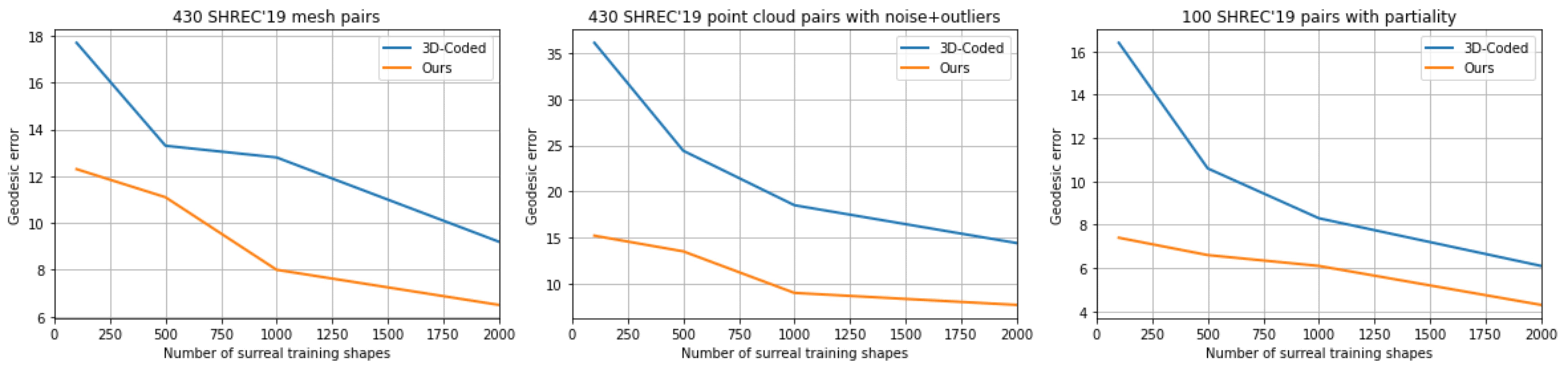
Figure 5: Number of training shapes and corresponding geodesic error on SHREC19 and its variants. Since we perform partial (source) to full (target) shape matching, the evaluation in the last graph only consists of a subset.

5.1 Effect of training data

We gradually increase the amount of training data and compare the correspondence accuracy across Scenario 1, Scenario 3 and Scenario 4 from Table. 2 in the main paper respectively. We construct four training sets consisting of 100, 500, 1000 and 2000 shapes from the SURREAL dataset [6]. Our motivation behind this study is to demonstrate the efficacy of our approach in settings with paucity of training data. To this end, we compare with the closest supervised baseline, 3D-CODED [6], and show that in spite of being supervised, our approach needs significantly less training data, fractions to be precise. Our approach and the baseline are trained with the same hyper-parameters as previously discussed.

Discussion: Across three scenarios, we observe that our approach consistently outperforms the baseline irrespective of the number of samples in the training set as shown in Figure 5. Interestingly, in Scenario 3, where we introduce corruption to the data in the form of outliers, our approach achieves an error when trained on 100 shapes that is comparable to 3D-CODED trained on 2000 shapes. Finally, we observe over a two-fold improvement in performance in the partial setting with 100 training shapes. We posit that a stronger conditioning of the latent embedding through SDF regularization and learning a volumetric map, which is independent of the underlying geometry to be a possible reason behind this observation.

5.2 Comparison to Oracle baselines

We compare our approach with three baselines, namely, 3D-CODED [6], Diff-FMaps [12] and CorrNet3D [26]. The three aforementioned baselines are trained on 230k SURREAL shapes [6] and thereby referred to as Oracle baselines. However, we stress again that we use our pre-trained network discussed in the main paper, trained on 2k SURREAL shapes.

We compare our method to the baselines by varying the level of corruption to data, across experimental settings studied in the main paper. To that end, we further subdivide this study in two experimental settings. First, we consider the variant of FAUST consisting of point clouds with clutter points. Second, we evaluate on the variant of SHREC’19 involving point clouds with noise and outliers respectively. For the first case, we use 15%, 25% and 30% clutter points in contrast to 20% of the total points discussed in the main paper. Similarly, for the second case, we vary the standard deviation of the Gaussian noise added to the surface between 0.5% and 25%, in contrast to 10% discussed in the main paper. Furthermore, for the second case, we add a stronger Gaussian Noise with standard deviation $\sigma=0.1$ to 20% of the points in the point cloud.

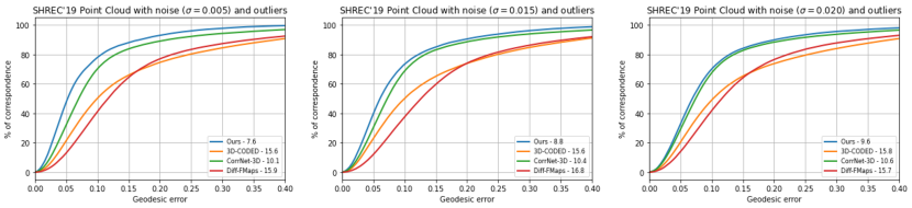
Figure 6: Quantitative comparison for matching point clouds with varying levels of noise. Our method is trained on 2000 training shapes while all the Oracle baselines are trained on 230k shapes.

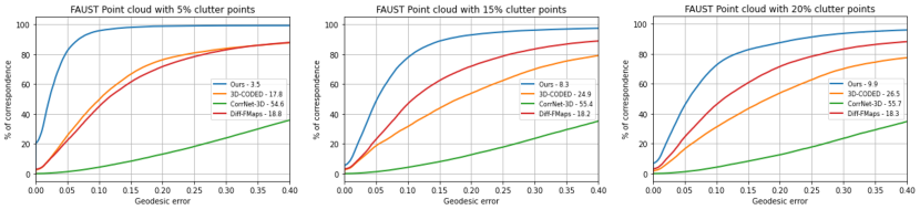
Figure 7: Quantitative comparison between our method and different baselines for matching point clouds in the presence of varying levels of clutter points. Our method is trained on 2000 training shapes while all the baselines are trained on 230k shapes.

Discussions: Our results are summarized quantitatively through geodesic accuracy graphs [8] in Figure 6 and Figure 7 respectively. Consistent with our observation in the main paper, our method shows high resilience towards noise and imperfection in data. Our aim of reducing the amount of noise is to show that performance of existing state-of-the-art methods rapidly degrades even in the presence of negligible imperfection in the data.

6 Qualitative results

Finally, we show qualitative results across different benchmarks, namely the noisy point cloud variant of SHREC’19 mentioned in our main paper, additional qualitative examples of scanned point clouds from CMU Panoptic dataset [7], animal shapes from Deforming Things 4D [10] and real-world scans of humans in clothing with registration artifacts from CAPE Scans dataset [11].

6.1 SHREC’19 Point clouds with outliers

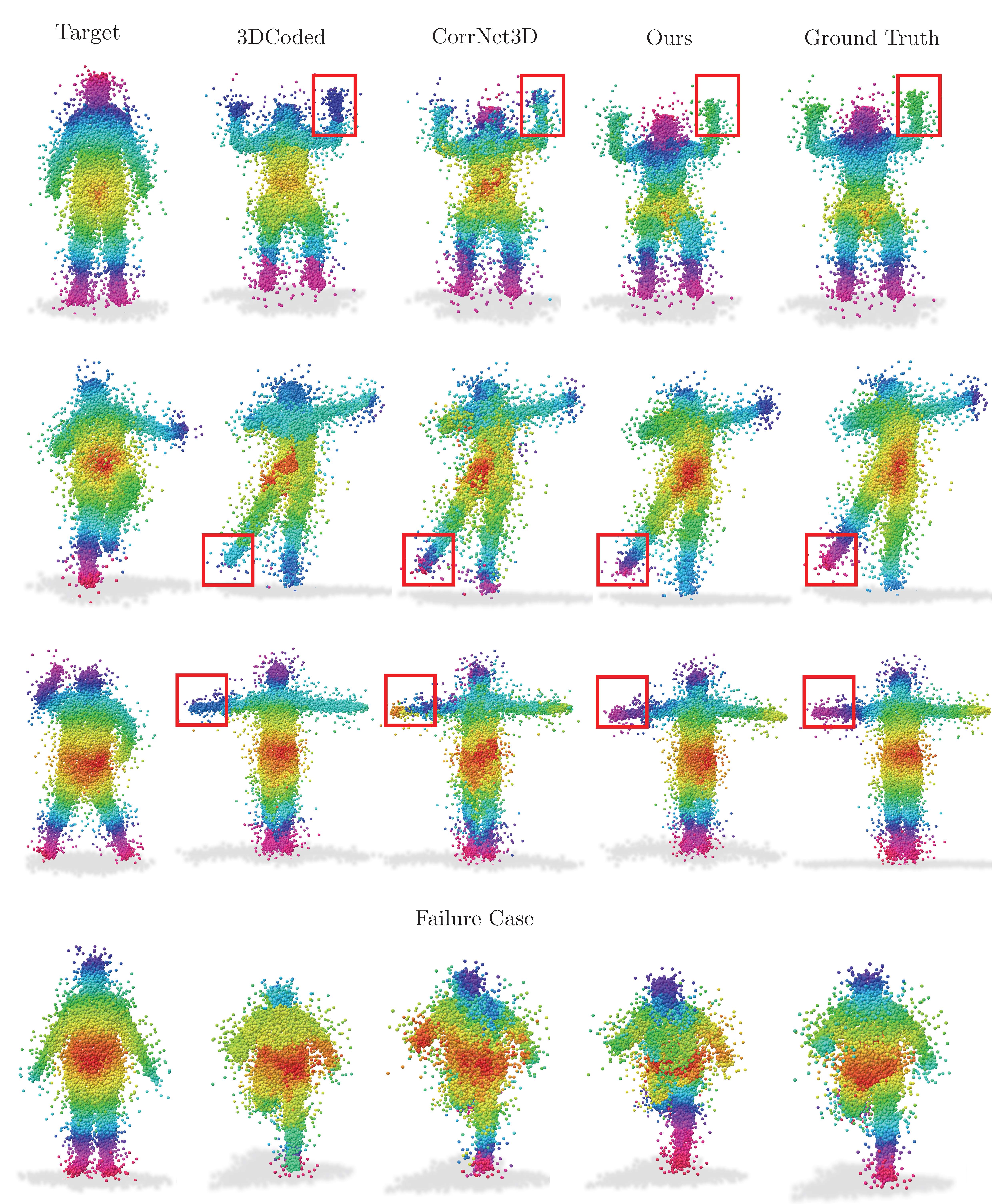
Figure 8: Additional qualitative results of our approach and the baselines 3DCoded [6], CorrNet3D [26] on SHREC’19 point clouds with outlier introduced in the main paper. For ease of observation, we highlight stark differences in map quality in red. In the final row, we also report a failure case of our approach.

6.2 Point Clouds from CMU Panoptic dataset

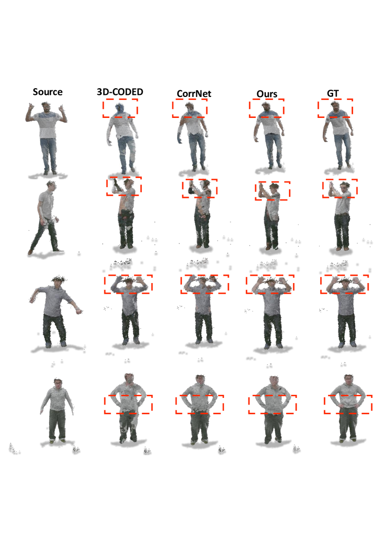
Figure 9: Additional qualitative results on CMU Panoptic dataset through texture transfer. Stark differences are highlighted using a bounding box for better visualization. Last row depicts a failure case of our method.

6.3 Deforming Things 4D

For the sake of completeness, we report additional qualitative results on inter-class point clouds consisting of animals from the Deforming Things 4D dataset [10]. This dataset consists of point clouds with self-occlusion and partiality, emulated through Blender. Please note that unlike previous cases, there is no ground truth information available for inter-class shapes. For our qualitative example, we consider Cow, Bear, Fox and Deer classes. Our choice is based on large inter-class variability and non-isometry. All methods are trained on SMAL dataset [28] as mentioned in the main paper.

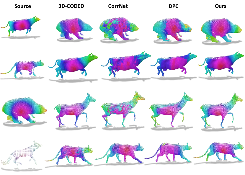
Figure 10: Additional qualitative results on Deforming Things 4D animals dataset through color transfer. Our approach shows better qualitative correspondence for large non-isometry between point clouds.

6.4 Clothed humans : CAPE Scans

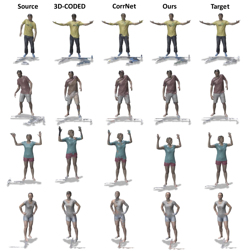
Figure 11: Additional qualitative results on clothed humans from CAPE scans [11] consisting of noisy meshes with outliers.

7 Limitations

While our method is largely robust through learning a volumetric map with strong regularisations, similar to all approaches that purely learn from extrinsic information, our approach suffers from generalization to unseen poses as depicted in the last row of Figure 8. This issue can in part be attributed towards the ill-posed problem of learning an embedding space purely from Cartesian coordinates. However, our current framework of joint learning of latent spaces by continuous functions opens possibilities for descriptor learning alongside purely extrinsic information. Another notable failure case of our method occurs at the area of self-intersection as depicted in the last row of Figure 9. Making our approach robust to self-intersections is also an interesting future work.

References

- [1] Aubry, M., Schlickewei, U., Cremers, D.: The wave kernel signature: A quantum mechanical approach to shape analysis. pp. 1626–1633 (11 2011). https://doi.org/10.1109/ICCVW.2011.6130444
- [2] Deng, Y., Yang, J., Tong, X.: Deformed implicit field: Modeling 3d shapes with learned dense correspondence. In: Proceedings of the IEEE/CVF Conference on Computer Vision and Pattern Recognition. pp. 10286–10296 (2021)
- [3] Donati, N., Sharma, A., Ovsjanikov, M.: Deep geometric functional maps: Robust feature learning for shape correspondence. In: 2020 IEEE/CVF Conference on Computer Vision and Pattern Recognition (CVPR). IEEE (Jun 2020). https://doi.org/10.1109/cvpr42600.2020.00862, https://doi.org/10.1109/cvpr42600.2020.00862
- [4] Eisenberger, M., Lähner, Z., Cremers, D.: Smooth shells: Multi-scale shape registration with functional maps. 2020 IEEE/CVF Conference on Computer Vision and Pattern Recognition (CVPR) pp. 12262–12271 (2020)
- [5] Eisenberger, M., Toker, A., Leal-Taixé, L., Cremers, D.: Deep shells: Unsupervised shape correspondence with optimal transport. arXiv preprint arXiv:2010.15261 (2020)
- [6] Groueix, T., Fisher, M., Kim, V.G., Russell, B., Aubry, M.: 3d-coded : 3d correspondences by deep deformation. In: ECCV (2018)
- [7] Joo, H.e.a.: Panoptic studio: A massively multiview system for social interaction capture. TPAMI (2017)
- [8] Kim, V.G., Lipman, Y., Funkhouser, T.: Blended intrinsic maps. ACM Transactions on Graphics 30(4), 1–12 (Jul 2011). https://doi.org/10.1145/2010324.1964974, https://doi.org/10.1145/2010324.1964974
- [9] Lang, I., Ginzburg, D., Avidan, S., Raviv, D.: DPC: Unsupervised Deep Point Correspondence via Cross and Self Construction. In: Proceedings of the International Conference on 3D Vision (3DV). pp. 1442–1451 (2021)
- [10] Li, Y., et al.: 4dcomplete: Non-rigid motion estimation beyond the observable surface. ICCV (2021)
- [11] Ma, Q., et al.: Learning to Dress 3D People in Generative Clothing. In: CVPR (2020)
- [12] Marin, R., Rakotosaona, M.J., Melzi, S., Ovsjanikov, M.: Correspondence learning via linearly-invariant embedding. Proc. NeurIPS (2020)
- [13] Melzi, S., Marin, R., Rodolà, E., Castellani, U., Ren, J., Poulenard, A., Wonka, P., Ovsjanikov, M.: Shrec 2019: Matching humans with different connectivity. In: Eurographics Workshop on 3D Object Retrieval. vol. 7 (2019)
- [14] Melzi, S., Ren, J., Rodolà, E., Sharma, A., Wonka, P., Ovsjanikov, M.: Zoomout: Spectral upsampling for efficient shape correspondence. ACM Trans. Graph. 38(6) (nov 2019). https://doi.org/10.1145/3355089.3356524, https://doi.org/10.1145/3355089.3356524
- [15] Ovsjanikov, M., Ben-Chen, M., Solomon, J., Butscher, A., Guibas, L.: Functional maps: a flexible representation of maps between shapes. ACM Transactions on Graphics (TOG) 31(4), 1–11 (2012)
- [16] Park, J.J., Florence, P., Straub, J., Newcombe, R., Lovegrove, S.: Deepsdf: Learning continuous signed distance functions for shape representation. In: Proceedings of the IEEE/CVF Conference on Computer Vision and Pattern Recognition. pp. 165–174 (2019)
- [17] Ren, J., Poulenard, A., Wonka, P., Ovsjanikov, M.: Continuous and orientation-preserving correspondences via functional maps. ACM Trans. Graph. 37(6) (dec 2018). https://doi.org/10.1145/3272127.3275040, https://doi.org/10.1145/3272127.3275040
- [18] Rodolà, E., Cosmo, L., Bronstein, M.M., Torsello, A., Cremers, D.: Partial functional correspondence. Computer Graphics Forum 36(1), 222–236 (Feb 2016). https://doi.org/10.1111/cgf.12797, https://doi.org/10.1111/cgf.12797
- [19] Rodolà, E., Cosmo, L., Bronstein, M.M., Torsello, A., Cremers, D.: Partial functional correspondence. In: Computer Graphics Forum. vol. 36, pp. 222–236. Wiley Online Library (2017)
- [20] ROHATGI, V.: An introduction to probability theory and mathematical statistics (1979)
- [21] Sharma, A., Ovsjanikov, M.: Weakly supervised deep functional maps for shape matching. In: Larochelle, H., Ranzato, M., Hadsell, R., Balcan, M., Lin, H. (eds.) Advances in Neural Information Processing Systems 33: Annual Conference on Neural Information Processing Systems 2020, NeurIPS 2020, December 6-12, 2020, virtual (2020), https://proceedings.neurips.cc/paper/2020/hash/dfb84a11f431c62436cfb760e30a34fe-Abstract.html
- [22] Sharp, N., Attaiki, S., Crane, K., Ovsjanikov, M.: Diffusionnet: Discretization agnostic learning on surfaces (2021)
- [23] Sharp, N., Crane, K.: A Laplacian for Nonmanifold Triangle Meshes. Computer Graphics Forum (SGP) 39(5) (2020)
- [24] Sitzmann, V., Martel, J., Bergman, A., Lindell, D., Wetzstein, G.: Implicit neural representations with periodic activation functions. Advances in Neural Information Processing Systems 33 (2020)
- [25] Xiao, B., Wu, H., Wei, Y.: Simple baselines for human pose estimation and tracking. In: European Conference on Computer Vision (ECCV) (2018)
- [26] Zeng, Y., Qian, Y., Zhu, Z., Hou, J., Yuan, H., He, Y.: Corrnet3d: Unsupervised end-to-end learning of dense correspondence for 3d point clouds. In: IEEE/CVF Conference on Computer Vision and Pattern Recognition (CVPR) (2021)
- [27] Zheng, Z., Yu, T., Dai, Q., Liu, Y.: Deep implicit templates for 3d shape representation. In: Proceedings of the IEEE/CVF Conference on Computer Vision and Pattern Recognition. pp. 1429–1439 (2021)
- [28] Zuffi, S., Kanazawa, A., Jacobs, D., Black, M.J.: 3D menagerie: Modeling the 3D shape and pose of animals. In: IEEE Conf. on Computer Vision and Pattern Recognition (CVPR) (Jul 2017)