An Automated Pipeline for Ultra-Violet Imaging Telescope (UVIT)

Abstract

We describe a versatile pipeline for processing the data collected by the Ultra-Violet Imaging Telescope (UVIT) on board Indian Multi-wavelength astronomical satellite ASTROSAT.The UVIT instrument carries out simultaneous astronomical imaging through selected filters / gratings in Far-Ultra-Violet (FUV), Near-Ultra-Violet & visible (VIS) bands of the targeted circular sky field ($\sim$ 0.5 deg dia). This pipeline converts the data (Level-1) emanating from UVIT in their raw primitive format supplemented by inputs from the spacecraft sub-systems into UV sky images (& slitless grating spectra) and associated products readily usable by astronomers (Level-2). The primary products include maps of Intensity (rate of photon arrival), error on Intensity and effective Exposure. The pipeline is open source, extensively user configurable with many selectable parameters and its execution is fully automated. The key ingredients of the pipeline includes – extraction of drift in pointing of the spacecraft, and disturbances in pointing due to internal movements; application of various corrections to measured position in the detector for each photon - e.g. differential pointing with respect to a reference frame for shift and add operation, systematic effects and artifacts in the optics of the telescopes and detectors, exposure tracking on the sky, alignment of sky products from multi-episode exposures to generate a consolidated set and astrometry. Detailed logs of operations and intermediate products for every processing stage are accessible via user selectable options. While large number of selectable parameters are available for the user, a well characterized “standard default” set is used for executing this pipeline at the Payload Operation Centre (POC) for UVIT and selected products are archived and disseminated by the Indian Space Research Organization (ISRO) through its ISSDC portal.

swarna@tifr.res.in

Received: date / Accepted: date

04 October 2021

1 Introduction

The ASTROSAT is the first Indian astronomical space mission which covers a wide range of the electromagnetic spectrum (Agrawal, 2006; Singh et al., 2014). This satellite carried five major scientific instruments to provide a platform for multi-wavelength astronomy from a low earth orbit with a small inclination to the equator. Four instruments covered different energies of soft to hard X-ray astronomy while the fifth one, Ultra-Violet Imaging Telescope (UVIT), enabled astronomical measurements over wide instantaneous field of view with high angular resolution, in the ultraviolet region. A summary of characteristics for each of these 5 instruments on board ASTROSAT are presented in Table 1. The primary aim of UVIT is to simultaneously image the desired region of the sky in Far-Ultra-Violet (FUV; 1300 – 1800 Å) and Near-Ultra-Violet (NUV; 2000 – 3000 Å) bands for a field of $\sim$ 28^′ diameter with a resolution $\sim$ 1.5^′′ (Tandon et al 2017a & 2017b). The telescope for NUV band also provided for imaging in optical / visible band (VIS; 3200 – 5500 Å), whose primary aim was to provide improved aspect of the telescope bore site every second. All three bands simultaneously view almost identical region of the sky. More details of UVIT and its in-orbit performance are presented in Tandon et al. (2017c) and references therein. The NUV band went non-functional on March 30, 2018 and remained so despite multiple attempts to revive it.

Table 1: Scientific experiments on board Indian multi-wavelength astronomical satellite ASTROSAT

Instrument	Ultra-Violet	Soft Xray	Large Area	Cadmium-Zinc-	Scanning Sky
	Imaging	Telescope	Xenon	Telluride	Monitor
	Telescope	(SXT)	Proportional	Imaging	(SSM)
	UVIT		Counter	Telescope
			(LAXPC)	CZTI)
Waveband	Far UV: 130-180 nm	Soft X-ray:	Soft & Hard	Hard X-ray:	Soft & Hard
	Near UV: 200-300 nm	0.3 - 8 keV	X-ray:	25 - 150 keV	X-ray :
	Visible: 320-550 nm		3 - 100 keV		2.5 - 10 keV
Field of View	$\sim$28 arc-min	$\sim$40 arc-min	0.9 deg$\times$0.9 deg	4.6 deg$\times$4.6 deg	22-27 deg$\times$
					100 deg
Optics	Twin Ritchie Chretian	Conical foil	Collimator	2-D coded	1-D coded
	2-mirror system	(Wolter-I)		mask	mask
		Mirrors
Detector	Photon	X-ray CCD	Proportional	CdZnTe	Position
	Counting	at the	Counter	Arrays	sensitive
	(Intensified)	focal plane			Proportional
	CMOS imagers				Counter
Angular	1.2-1.5 arc-sec	2 arc-min	$\sim$1-5 arc-min	8 arc-min	$\sim$10-13 arc-min
Resolution	(in Far &		(in scan		along coding
	Near UV)		mode)		axis & 2.5
					deg across
Energy	10-50 nm	90 eV at 1.5 keV	12-15%	6% at	25%
Resolution	as per filter	136 eV at 5.9 keV	in 22-60 keV	100 keV	at 6 keV
	selection
Geometrical	1250	250	10,800 (total	976	173
Collection	for each of the		for 3		(total for
Area (cm2)	3 wavebands		identical		3 units)
			units)
Effective	$\sim$10 for Far	90 at 1.5 keV	6000	415	11
Area (cm2)	UV band;		at 5-20 keV	photometric;	at 2.5 keV;
	$\sim$10 for Near		(total for 3	335	51
	UV band;		identical	spectroscopic	at 5 keV;
	$\sim$40 for Visible		units)		(total for
	band;				3 units)
Time	2 milli-sec	$\sim$2.4 sec for	10 micro-sec	20 micro-sec	0.1 milli-sec
Resolution		full field;
		$\sim$0.28 sec for
		central area
Sensitivity	20 mag (5$\sigma$)	$\sim$10-13 erg cm-2	1 milli-Crab	20 milli-Crab	$\sim$28-40 milli-
	in 160 sec for	sec-1 (5$\sigma$)	(3$\sigma$) in	(5$\sigma$) in	Crab (3$\sigma$)
	for Far UV	in 20,000 sec	1,000 sec	10,000 sec	in 600 sec
Total Mass (kg)	230	70	419	56	65.5

The subject matter of this paper is the automated pipeline for processing of the raw data received from the instrument and the spacecraft to produce images for FUV and NUV in standard units. The processing involves two separate steps. The first step, called L1 (Level-1), processes the telemetery data to provide a bundle of data for each target of observation. The L1 data bundle for UVIT consists of Science (Imaging) data from all 3 Detectors and Auxilliary (Aux) data containing inputs regarding UVIT Filters and various information from Spacecraft Systems, e.g. time calibration, attitude of satellite reference axes, position in orbit, gyro signals, and house keeping information. The second process, called L2 (Level-2), uses the bundle provided by L1 to make images for FUV and NUV in standard units for use by astronomers. The process L1 is implemented at a centre of Indian Space Research Organization (ISRO), while the process L2, which is theme of this paper, is implemented at UVIT-Payload Operation Centre (UVIT-POC) at Indian Institute of Astrophysics, Bangalore. It is ISRO’s exclusive right & responsibility to operate, maintain and upgrade the archives for disseminating all scientific data products from UVIT (which includes both L1 & L2).

The motivation for this paper is as follows. It provides an authentic description of processes involved in the translation from the Level-1 to the Level-2, which uses this pipeline. The ISRO’s archive hosts the L2 products generated using a “default” set of selectable parameters which are optimal for catering to most general users. The present work not only explains the implications of these selections, but also provides details about various additional options some of which could be useful to researchers with specific science aim. In addition, for future refinements of the pipeline, this work provides the basic reference.

Structure of this paper is as follows. In Section 2, we present a brief overview of imaging operations with UVIT and the complete end-to-end flow of data beginning from their collection to the final products that are ready for scientific analysis and interpretation by astronomers. In Section 3, detailed description of all the processing steps involved in generating Level-2 starting from Level-1 data is presented (hereafter referred to as UVIT Level-2 Pipeline, UL2P). This section first describes the higher level structure of the software, and details of the lower level structure follow subsequently. Section 4 contains experience during commissioning the pipeline, selected sample results, success rates and yields of UL2P and their general archiving details. Section 5 presents a summary along with comments on possible further improvements for future.

2 Overview

2.1 Imaging with UVIT

The imaging components of UVIT include optics, detectors and filter wheels. The optics consists of twin identical Ritchey-Chretian telescopes as shown in Fig. 1. (more details can be found in Kumar et al 2012 a).

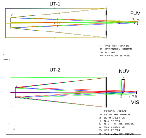
Figure 1: Optical layout of the two UVIT Telescopes, UT-1 and UT- 2, each employing a pair of Primary & Secondary mirrors. The UT-1 is dedicated for the Far-UV (FUV) band. The UT-2 feeds the Near-UV (NUV) band via reflection of a beam-splitter and the Optical (VIS) band through it.

The detector system for each of the 3 bands consist of intensified C-MOS imager (Star-250; 512$\times$512 pixels), whose gain can be configured through its high voltage settings. While a high gain deploys Photon Counting mode (PC; $\sim$ 29 frames/s for the full field) used for the two UV bands, a low gain effects Integration mode (INT; $\sim$ 1 frame/s) used for the VIS band. Details of these modes are available in the Appendix-1 (Sec. A1.1).

A single clock (among the 3 bands) is selected for the operational ease of inter-band time alignment.

The Filter Wheel Drive system of each band positions the selected filter (or grating) and is parked at a light blocking position when not in use.

The electronic controller for each band configures and operates the detector read out system. The key selections include : (a) size of the sky field - full field (512$\times$512 pixels) or a smaller square window (100$\times$100 / 150$\times$150 / 200$\times$200 / 300$\times$300 / 350$\times$350) for obtaining higher frame-rates, roughly in inverse proportion the number of pixels read ; & (b) the imaging mode (PC / INT).

The imaging sessions are scheduled only during dark part of any orbit to avoid scattered solar radiation. Every planned sky field undergoes detailed checks for its safety against overexposure due to any unacceptably bright object in the field or moon within a cone of defined half angle from the axis. Additionally, onboard safety measures with autonomous swift action ensure detector safety against accidental exposure to bright field.

The spacecraft operations usually translate observations of a specific astronomical target, with the filter and window size, of a typical science proposal into a sequence of smaller segments of imaging sessions, i.e. Episodes, spread over multiple orbits, as a single orbit can support imaging for a maximum of $\sim$ 2000 seconds, primarily due to the requirement of dark side of the orbit, and other factors like angle constraint to avoid earth occultation, South Atlantic Anomaly etc can further curtail this duration.

2.2 End to end data flow

The Fig. 2 shows the scheme of onboard interfaces between the ASTROSAT spacecraft and UVIT for control of operations using commands as well as collection of data to be communicated to the ground station. In addition to planned operations, the spacecraft systems also process emergency situations and guides UVIT to a safe condition. The data collected correspond to sky images, status & settings of various parameters of subsystems and health monitoring.

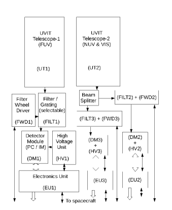
Figure 2: Schematic of the UVIT Payload. The telescope UT1 (UT2 & a Beam Splitter) feeds all sub-systems for the FUV (NUV & VIS) band/(s). The sub-systems represent functionalities including the selection of desired Filter (or Grating), configuration of Detector read out & settings of its High Voltages, and two way data communications with the spacecraft.

A block diagram displaying data flow and interconnections on ground is presented in Fig. 3. After the required processing at the ISRO’s ground segment systems, the data for UVIT are provided as FITS files called Level-1 data. These includes Science Data from the three detectors, and all the additional information on UVIT and the SC (named Aux Data) necessary for the next processing step. All the parameters of the detectors are made available in the Science Data, and the Aux Data provides status & positions of the three filter wheels, time calibration table, orbital position, velocity, attitude information of the reference axes of the satellite, data from Gyros, and housekeeping information, at appropriate sampling rates.

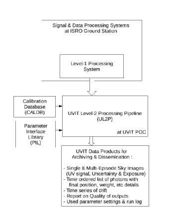
Figure 3: UVIT / ASTROSAT Ground Segment Systems. The UVIT Payload Operation Centre (POC) executes the Level-2 Pipeline using various inputs and generates the astronomer ready Sky Image Products & other outputs for archiving and dissemination.

Each observing session (Episode, for a specific band, filter & window setting), is no longer than $\sim$ 2000 s, i.e. dark part of an orbit. All the Level-1 data products (Science Data & Aux Data) for all the Episodes for a target are organized into a single bundle named as “merged Level-1”. In the merged bundle Science Data for each band are assembled in individual directories and all the Aux Data are assembled in another directory. The Level-2 pipelines uses the directories of Science Data and Aux Data along with the calibration data base for generating the final images in standard units and coordinates. The data on raw images are provided by Science Data, data on the filters and orientation of the satellite are provided by Aux Data. Data on variation of sensitivity over the field and geometrical distortions are taken from the calibration data base. Details of operations executed in the pipeline are described in Section 3.

3 Level-2 Pipeline

This section gives a full description of the pipeline. The section is divided in two parts: in the first part functionality of the pipeline is described fully, and in the second part the actual implementation is described. A list of acronyms used in this document as well as frequently used names for a few key user selectable parameters is presented in Table 2. Additionally, a complete list of all parameters are available at the very end (Appendix-11). For most readers the functionality of the pipeline would suffice without going into the detailed description, which is full of many intricate technical details, unless they want to use / run the pipeline themselves for generation of the images.

Table 2: List of frequently used acronyms, names and selectable parameters referred to in this document.

Serial	Acronym / Name	Expanded form /
No.	/ Selectable parameter	Description
	Acronym :
1	CAL_DB	Calibration Database
2	CR	Cosmic Rays
3	CRC	Cyclic Redundancy Check
4	ENT	Effective Number of Photon
5	FITS	Flexible Image Transport System
6	FUV	Far-UltraViolet band of UVIT
7	GTI	Good Time Interval
8	ICRS	International Celestial Reference System
9	INT	INTegration Mode of imaging
10	ISRO	Indian Space Research Organization
11	ISSDC	Indian Space Science Data Centre
12	L1	Level-1 data (input for the pipeline)
13	L2	Level-2 data (output of the pipeline)
14	L2_PC	Level-2 Sky Imaging chain for data
		collected in Photon Counting (PC) mode
15	L2_INT	Level-2 Sky Imaging chain for data
		collected in Integration (INT) mode
16	MCP	Micro-Channel Plates (used as
		Intensifier in the Detector Module)
17	MJD	Modified Julian Date
18	mL1	Merged Level-1 data bundle (input for the
		pipeline; provided by ISRO / ISSDC)
19	NUV	Near-UltraViolet band of UVIT
20	OE	Other Episode/s (other than the Reference Episode
		among the “group” of Episodes to be combined,
		with identical Band, Filter & Window configuration)
21	PC	Photon Counting Mode of imaging
22	PIL	Parameter Interface Library
23	POC	Payload Operation Centre (located at the Indian
		Institute of Astrophysics, Bangalore)
24	PSF	Point Spread Function
25	RA_INT	Level-2 Relative Aspect chain for data
		collected in Integration (INT) mode
26	RA_PC	Level-2 Relative Aspect chain for data
		collected in Photon Counting (PC) mode
27	RAS	Relative Aspect Series (time series of 3 variables
		quantifying drift; Roll-Pitch-Yaw / X-Y-$\theta$)
28	RE	Reference Episode (with longest exposure time)
		among the “group” of Episodes to be combined,
		each with identical Band, Filter & Window
		configuration
29	RF	Reference Frame; defines the instance of time for
		an Episode, with respect to which drift corrections
		are measured & applied to frames at future times
30	SAA	South Atlantic Anomaly
31	SC	Spacecraft
32	SSM	Scanning X-ray Sky Monitor
33	UL2P	UVIT Level-2 Pipeline
34	USNO	United States Naval Observatory (catalogue of
		stars)
35	UTC	Universal Time Clock
36	UV	Ultra-Violet
37	UVIT	Ultra-Violet Imaging Telescope
38	VIS	Visible (VIS) band of UVIT
	Name / Selectable parameter :
1	Aux	Auxiliary data (from spacecraft sub-systems)
2	Episode	Smallest unit of imaging session as per mission
		operations; corresponding data consist of time
		series of frames read out at a planned rate
3	EXP_TIME	Total effective Exposure Time (seconds) based on
		no. of frames contributing to the product
4	Exposure	2-D Array, its elements hold no. of frames
		exposed with valid pixels of the detector
5	N_acc	No. of successive VIS frames to be stacked for
		generating individual accumulated images,
		‘Acc_frame’ (from which star are identified for
		drift tracking; used in RA_INT chain)
6	N_avg	Centroids of detected stars from N_avg successive
		accumulated images (Acc_frames) are combined
		to select a wider time bin for drift computation
	(used in RA_INT chain)
7	N_combine	(1) No. of successive NUV /FUV frames to be
		accumulated for generating time series of images,
		‘Comb_frame’, from which drift is extracted
		(used in RA_PC chain);
		(2)Division of Episode into multiple pseudo-
		Episodes, each consisting of N_combine
		consecutive frames (when “pseudo-Episode”
		option is used in L2_PC chain);
8	N_p	No. of packets containing image data in a frame
9	ObsID	Observation ID identifies an unique sky pointing
		towards a target
10	pseudo-Episode	Part of an Episode when divided into multiple
		data chunks (each with N_combine frames)
11	Sig	2-D array, with elements holding accumulated
		ENPs from drift corrected frames
12	Signal	2-D array, sky image in “counts/sec” unit
13	Uncertainty	2-D array, with elements holding statistical
		uncertainty from no. of photon of events
		contributing to the pixel (in “counts/sec” unit)
14	utcFlag	Switch to select either Universal Time Clock or
		UVIT’s Master Clock for timing

3.1 Functionality

This sub-section provides a qualitative description of the operations carried out by the pipeline for generating the astronomer ready output products. This includes the primary aim, various inputs and the key processing steps. The terminology used here are as follows. The term “Step” has been introduced at the very highest level of description for ease of comprehension. A “Chain” refers to a completely stand alone sequence of smaller processing “Block”-s. The functionality of several Blocks used for different imaging modes and/ or Chains are similar, hence they have been implemented as “Modules” callable with appropriate selection of switches. The codes for remaining Blocks are embodied within respective Chains. Individual Chains are described in later sections 3.2.1, 3.2.2 & 3.2.3. While a few brief generic comments about Modules appear in section 3.2.7, individual Modules are described in Appendix 1 (Sec A1.1, to A1.20). The functionality of Blocks that are not Modules are given within the description of Chains.

3.1.1 Primary Aim of Level-2 Pipeline

The UVIT Level-2 Pipeline (UL2P) is designed to translate ISSDC /ISRO provided Level-1 data (mL1) into science ready products in astronomer friendly format, utilizing instrument calibration database (CAL_DB) as well as user settings of selectable parameters & switches (PIL) (see Fig 3). The primary products include the two UV sky image arrays as detected photon count rates in standard coordinate system (Right Ascension – Declination J2000) as well as primitive detector coordinate system (X-Y axes of the sensor) for every imaging Episode. The corresponding Uncertainty Arrays and sky Exposure Arrays are also generated. The subsidiary products include time series of spacecraft drift, photon centroid list for the image with flat field weight, etc. In addition to the above products for every Episode of observation, similar products are generated, by combining data for all the Episodes, for the total exposure (in all the orbits) with identical Filter-Window combination. The above is achieved through an one time run of a fully automated Driver Scheme, using a single configuration file for user selections.

3.1.2 Input Data

There are three types of inputs required for running the pipeline, viz., the bundled Level-1 data (merged Level-1; mL1), the calibration database (CAL_DB) and the user settings of all selectable parameters and switches (Parameter Interface Library; PIL).

The mL1 represents collection of all data pertaining to one specific pointing of the spacecraft to the astronomical target (referred to by an unique Observation ID, ObsID). It consists of science data from all sky exposures executed by UVIT during that pointing as well as auxiliary data from the spacecraft systems (e.g. orbit & attitude information). The science data are packed as a sequence of “frame”-s, one for each individual short exposure. Their content depend on the mode of operation of the detector, viz., Integration (INT; used for VIS band; $\sim$ 1 frame per sec) or Photon Counting (PC; used for NUV & FUV bands; $\sim$ 29 fps). While the raw pixel values of the entire field (512x512) are preserved for INT mode, centroids (computed onboard) of individual detected photons constitute the frame for the PC mode. More details about exact contents of these data are available elsewhere (Appendix-1, Sec. A1.1).

An “Episode” of exposure in any band is defined as one continuous imaging session with a specific selection of filter and window size. Thus, an Episode can either last the whole usable dark-side of an orbit or a fraction of it in case the settings are changed. There is an option in the pipeline to divide the imaging duration of one Episode into multiple equal segments for processing independently. These segments are referred to as “Pseudo-Episode” individually. The nomenclature of grouping of science data used here is displayed in Fig. 4. The CAL_DB contains organized datasets representing calibration arrays for each band (FUV, NUV & VIS) quantifying flat field correction across the detector, distortions, bad pixels, etc. The complete details of CAL_DB are presented in Appendix-5.

The PIL is a single configuration file containing numerical values of all selectable parameters and ON/OFF settings of various switches. While complete details are available in Appendix-11, a few key parameters are also listed in Table-2.

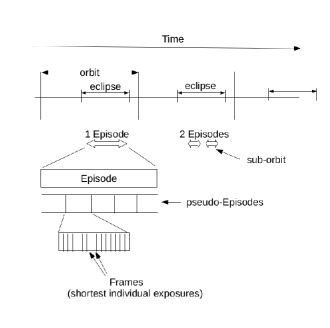
Figure 4: Nomenclature for data groupings. Each “orbit” corresponds $\sim$ 100 minutes - the time taken by the spacecraft to go around the Earth once. The term “eclipse” refers to that part of every orbit when the spacecraft is in the Earth’s shadow blocking the Sun. UVIT observations are mandatorily scheduled during eclipses for instrument safety. The entire eclipse duration could either be used for sky exposure with a fixed settings for data collection leading to a single “Episode” or the time can be sub-divided into 2 or more exposures (with different settings) as per scientific needs. The pipeline has an option to sub-divide the data collected during one Episode into multiple pseudo-Episodes. The imaging data collection during an Episode involves repeated read outs of the detector - data corresponding to an individual read out is called a “Frame”.

3.1.3 The Processing Steps

The generation of UV images from the inputs described above, involve the following main processing steps which are identical for NUV and FUV bands. 1) At first the drift of spacecraft pointing is estimated using stars detected in images captured in VIS frames (sampled $\sim$ 1 frame-per-sec, fps). There is an alternate provision for finding drift from NUV / FUV band data also in absence of VIS band data. 2) Next, individual UV frames are added to generate a cumulative image in the detector coordinates, after applying drift corrections and various instrumental corrections (which varies across the field of view) to the detected photons of each individual frame. Appropriate transformation is applied to generate the image in RA-Dec coordinates also. The corresponding Uncertainty to the UV image (from photon statistics) and the Exposure on the sky are also generated, which complete the set of image products. The above description is applicable for each single imaging session (Episode) lasting $\sim$ 2000 sec or less (see Fig. 5). 3) Image products from successive imaging sessions with identical combination of filter and window size (for the same UV band), are combined to generate the products for the total exposure by applying corrections for the relative shift and rotation determined using brigher UV stars detected in individual Episodes (described in a later sub-section named Driver Scheme, Sec 3.2.4; see Fig. 9).

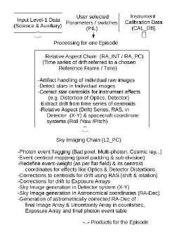
Figure 5: Schematic diagram showing generation of UV sky image corresponding to a single uninterrupted observing session called Episode. Starting with Level-1 data for the Episode along with UVIT calibration data (CAL_DB) & user selected options (PIL), two stand alone processing chains (Relative Aspect chain, RA_INT or RA_PC; & L2_PC) generate the output products. Actions in the first block (Relative Aspect chain to extract drift of the spacecraft) include : correcting for artifacts & detection of stars in raw VIS images for RA_INT (& similarly from UV images generated by stacking photon centroids, in case of RA_PC) applying corrections to star centroids for instrument effects (distortions), determine drift (shift & rotation) as a function of time (from centroids) in Detector coordinates and finally convert to spacecraft coordinates. The second block (Sky Imaging chain to generate UV sky image & other products) begins with input UV data (list of centroids of photon events), flags affected events for rejection, computes event weight to include flat field, applies corrections to centroids for various systematic effects of the instrument & drift (applicable for corresponding time instance) determined in the first block, to obtain true sky arrival directions of individual UV photons. The UV sky image is generated by accumulating individual photons in both the Detector and Astronomical coordinates directly. Corresponding Uncertainty (from photon statistics) as well as sky Exposure maps are also generated.

The first two steps, #1 & #2 above are stand alone processing chains named - (i) the Relative Aspect chain which generates a time series of drift relative to position at some reference time as defined by the corresponding Reference Frame; (ii) the Sky Image chain which generates astronomical images & associated products. As the exposures can be taken either in photon counting (PC) mode or in integration (INT) mode, each of the chains has two versions (accordingly the chains are designated as : RA_INT / RA_PC & L2_PC / L2_INT). The last step (#3) is called Driver Scheme which combines images & associated products (Exposure & Uncertainty Arrays) obtained from all the Episodes, corresponding to the same combination of filter and window, after aligning them to correct for relative shift and rotation.

The key functionalities of these chains and the Driver Scheme are summarized along with their implementation in the next section (Sec. 3.2). The chains in turn call various processing Modules, whose technical descriptions appear in Appendix-1.

3.2 Implementation

This subsection provides various details of implementation of the pipeline. First the processing chains RA_INT, RA_PC & L2_PC and the Driver Scheme are summarized, followed by the strategy for addressing the situation of data loss in the input bundle as well as handling of special situations. Finally general concepts behind the design of modules are presented (details of individual modules can be found in Appendix-1).

The figures displaying the processing blocks of various chains follow a convention to distinguish Modules from rest by shading the latter (Fig.s 6, 7 & 8). In addition the blocks which have rarely been turned on are identified in the respective captions for the figure.

3.2.1 Relative Aspect chain for Integration mode (RA_INT) :

The purpose of this chain is to obtain time series of instantaneous shift and rotation of the field, relative to the position at any chosen time or set of frames, every second or so. This chain operates on VIS band data which are collected in INT mode. The typical accuracy obtained is $\sim$ 0.1^′′ for the full field. The chain operates on data of one Episode at a time. Various steps of the processing are shown in Fig. 6 (RA_INT) and are described below in the sequence in which they are executed and the numbers in parenthesis refer to the block numbers in that figure.

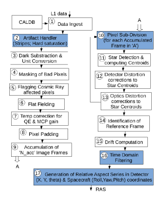
Figure 6: Schematic block diagram of the Relative Aspect chain for Integration mode (RA_INT). The block numbers 7 and 10 have never been turned on (except for testing & validation). The manual mode of star selection is not shown. The shaded blocks do not belong to any Module.

Data Ingest (1) : Import of all the user selected switch settings and values from a parameter file. Relevant data on calibration and on the exposure are taken from CAL_DB and mL1 respectively. These data are: a) from calibration: the tables /arrays of bad pixels, distortions, flat-field, dark & exposure template; b) from mL1: i) science data originating from the instrument: frames of INT mode images in selected band, and ii) auxiliary data from the S/C: aspect of S/C, time calibration, house keeping information on instrument health, good-time /bad-time flags. Handling of discontinuities and abnormal data. Removal of engineering grade science data collected during gradual ramping up of the highvoltages at the beginning of the Episode, as per safety protocol. Extraction of individual image frames.

Artifact Handler (2) : The unexpected artifacts in the image and saturated pixels are flagged here enabling further processing to ignore them.

Dark Subtraction & Unit Conversion (3) : Subtraction of ‘dark’ frame from each individual image frame followed by conversion of the signal values from “count per exposure” to “count per second” unit.

Masking of Bad Pixels (4) : Flagging of the locations corresponding to ‘Bad Pixel’-s in every image frame.

Flagging Cosmic Ray affected pixels (5) : Identification of Cosmic Ray affected pixels (in every image frame) and their flagging.

Flat Fielding (6) : Multiplicative correction for non-uniform response across the field applied to all image frames.

Pixel Padding (8) : Expansion of all images from 512$\times$512 to 600$\times$600 size by symmetrically adding pixels along all four sides populated with a flag. This enlargement allows accommodation of movement of the instantaneous sky field due to spacecraft drift over the duration of the Episode. While this functionality is not explicitly required in this Chain, the corresponding Module (& also the following processing steps) being common with the Sky Imaging Chain, this step is retained to keep the array dimensions compatible.

Image Accumulation (9) : Selection of time step for drift computation by accumulating and averaging selected number, N_acc, of successive image frames generating a series of accumulated frames, Acc_frame.

Detection of stars & finding Centroids (11) : Analysis of individual image Acc_frames to identify stars using an algorithm which uses dynamic threshold, distribution of light around local maxima and neighbourhood criteria. Computation of X & Y centroids for every detected star and intensity ordered tabulation.

Correction for Detector Distortion (12) : Application of additive corrections to the centroids of stars for the detector distortion.

Correction for Optics Distortion (13) : Application of additive corrections to the centroids of stars for the distortion due to telescope optics.

Identification of Reference Frame & Binning of time step (14) : Selection of timing reference for drift computation process, by identifying a particular Acc_frame to be the Reference Frame, RF (by skipping the initial N_skip number of Acc_frame-s). Beginning with the RF and till the end of the Episode, an additional level of binning of time step is carried out optionally, by averaging star centroids exytracted from N_avg number of successive Acc_frame-s. (For default usage, N_avg = 1).

Drift Computation (15) : Computation of time series of relative drifts (shifts along X & Y axes and a rotation about the central pixel) from the differences in centroids of matching stars tabulated for successive time samples. The centroids for multiple stars are used in a least square fitting scheme having a choice of either equal or intensity based weighting. A manual mode of inter active selection of stars is also available to mitigate rare situations arising due to residual artifacts in the image data unaddressed by the handler block (#2). Subsequent translation of these drifts for every time sample to the integral drifts, with respect to the timing reference corresponding to the Reference Frame.

Time Domain Filtering (16) : The time series of drift in three variables ($x_{shift}$, $y_{shift}$ & $\theta$) are low-pass filtered in time domain, with user selectable parameters for smoothening them.

Generation of Relative Aspect Series (17) : The time series of drifts are tabulated as Relative Aspect Series, RAS, in Detector ($X$, $Y$, $\theta$) as well as Spacecraft (Roll,Yaw,Pitch) coordinates systems as finalproduct from this RA_INT chain.

The Appendix-8 presents the directory structure of final products from the RA_INT chain.

3.2.2 Relative Aspect chain for Photon Counting mode (RA_PC) :

The aim of the RA_PC chain is identical to that for the RA_INT chain, but its functional details are different since it operates on the data collected in Photon Counting mode (e.g. when NUV or FUV data is used to obtain the time series of drift, Relative Aspect Series). This chain also operates on data of one Episode at a time. Various steps of the processing are shown in Fig. 7 (RA_PC) and are described below in the sequence in which they are executed.

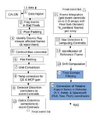
Figure 7: Schematic block diagram of the Relative Aspect chain for Photon Counting mode (RA_PC) The block number 8 has never been turned on (except for testing & validation). The shaded blocks do not belong to any Module.

Data Ingest (1) : Similar to the case of RA_INT (see above), except that the science data originating from selected band of the instrument operated in PC mode consist of a table with details of individual photon events detected in successive exposed frames in the Episode. These details (e.g. centroids) are generated from the raw frames, through on board processing. In this step, a master table of photon events along with relevant data is created.

Flagging of events in Bad Pixels (2) : A column is appended to the master table which holds the Bad Pixel flag. The events with their X & Y centroid coordinates overlapping with any of the bad pixels are flagged. Later processing steps ignores the flagged events.

Pixel Padding (3) : The centroid coordinates are modified to translate their range from (1 to 512) to (1 to 600) along each axis thereby effectively incorporating symmetric padding along all four sides. This allows accommodation of movement of the instantaneous sky field due to spacecraft drift over the duration of the Episode. Here again, this step is retained for compatibility of the shared Modules between the Relative Aspect & Sky Imaging Chains.

Rejection of Cosmic Ray affected frames (4) : Identification of individual frames affected by showers due to Cosmic Ray events and discarding all events in them. The process uses statistical distribution of number of events in all frames of the Episode and user selected parameters to arrive at the threshold value for flagging. This rejection is useful for dark fields where contribution of showers to the background of photon events can be a large fraction of the total. If the rejection is not desired, the parameters can be set accordingly.

Centroid Bias correction (5) : Application of corrections for systematic bias, due to use of a simple algorithm on board, to the centroid values.

Flat Fielding (6) : The ‘Effective Number of Photon’ (ENP) for every event is changed from its initial value of unity by application of multiplicative correction for non-uniform response across the field.

Unit Conversion (7) : The entries for all events are modified from ‘ENP per frame’ to ‘ENP per second’ unit.

Correction for Detector Distortion (9) : Application of additive corrections to the centroids of photon events for the detector distortion.

Correction for Optics Distortion (10) : Application of additive corrections to the centroids of photon events for the distortion due to telescope optics.

Frame Integration (11) : Transformation of centroid coordinates for all photons from (600, 600) range to (4800, 4800) to implement pixel sub-division. Generation of a time series of two dimensional sky image arrays, Comb_frame (4800$\times$4800), by accumulating photon events from selected number of consecutive frames (N_combine). The functionality of this selectable parameter N_combine for this RA_PC chain is equivalent to the parameter N_acc for RA_INT chain. The distinct nomenclature is chosen to emphasize the large difference in their typical values (N_acc $\sim$ 1; N_combine $\sim$ 30).

At this stage of processing of the RA_PC chain, 2-D sky images are available starting from PC modedata. Accordingly, the subsequent steps leading to extraction of drift are very similar to the corresponding steps of RA_INT.

Detection of stars & finding Centroids (12) : Similar to that for RA_INT chain (step #11) above.

Identification of Reference Frame & Binning of time step (13) : Similar to that for RA_INT chain (step #14) above.

Drift Computation (14) : Similar to that for RA_INT chain (step #15) above.

Time Domain Filtering (15) : Similar to that for RA_INT chain (step #16) above.

Generation of Relative Aspect Series (16) : Similar to that for RA_INT chain (step #17) above.

3.2.3 Sky Image chain for Photon Counting mode (L2_PC) :

The Sky Image chains L2_PC and L2_INT generate astronomical images for observations carried out in Photon Counting and Integration mode respectively . Primary aim of UVIT is to image in NUV and FUV bands, both of which are observed in the PC mode. Hence, the functionality of only the L2_PC chain is presented here, which is the more significant among the two versions.

The L2_PC chain processes data from one Episode and one band (NUV / FUV) at each instance. The Fig. 8 displays the schematic block diagram for this chain. Its steps are described below in the sequence of their execution. Certain steps here are similar to corresponding steps in the RA_PC chain described earlier.

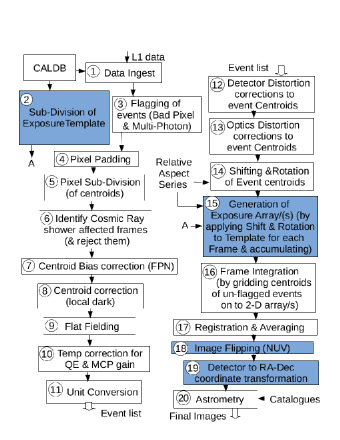
Figure 8: Schematic block diagram of the Sky Imaging chain for Photon Counting mode (L2_PC) The block numbers 8 and 10 have never been turned on (except for testing & validation). The shaded blocks do not belong to any Module.

Data Ingest (1) : Importing selected switch settings and parameters, calibration and exposure data, spacecraft aspect, time calibration, etc. as well as science data (see step #1 of RA_INT & RA_PC for details). Generation a master table of all photons along with their details for the entire Episode.

Creation of Exposure Template (2) : The master templates of sky exposure are created for every combination of band, mode and window size by carrying out pixel sub-division of corresponding arrays available from the CAL_DB. The resulting sky Exposure Template arrays are of 4800$\times$4800 size. In order to track true exposure of the sky on the detector, the relevant master array will be offset according to drift corrections applicable for the time instances and stacked together in a later processing block.

Flagging of events in Bad Pixels; & with Multi-Photon signature (3) : Flagging of events with centroids located within a Bad Pixel (similar to step #2 of RA_PC). Identification of potential multi-photon cases from event details along with user selected parameters and flagging them- this selection has never been used.

Pixel Padding (4) : Modification of the centroid coordinates of photon events by translating their range from (1 to 512) to (1 to 600) to accommodate spacecraft drift (similar to step #3 of RA_PC).

Pixel Sub-Division of centroids (5) : Transformation of centroid coordinates for all photons from (600, 600) range to (4800, 4800) by pixel sub-division.

Rejection of Cosmic Ray affected frames (6) : Identification and rejection of frames affected by Cosmic Ray showers (similar to step #4 of RA_PC).

Centroid Bias correction (7) : Application of corrections for systematic bias to the centroid values (similar to step #5 of RA_PC).

Flat Fielding (9) : Application of multiplicative correction for non-uniform response across the field (similar to step #6 of RA_PC).

Unit Conversion (11) : The entries for all events are modified from ‘ENP per frame’ to ‘ENP per second’ unit (similar to step #7 of RA_PC).

Correction for Detector Distortion (12) : Application of additive corrections to the centroids of photonevents for the detector distortion (similar to step #9 of RA_PC).

Correction for Optics Distortion (13) : Application of additive corrections to the centroids of photon events for the distortion due to telescope optics (similar to step #10 of RA_PC).

Corrections for drift (14) : Extraction of corrections for spacecraft drift applicable to individual frames by time interpolation of the corresponding Relative Aspect Series, RAS. The RAS should be available from a prior run of the Relative Aspect chain (RA_INT or RA_PC) covering the time duration of the Episode. Application of drift correction (involving 2 shifts & a rotation) to centroids of the individual photons.

Generation of drift corrected Exposure Array/(s) (15) : Application of drift corrections to a time series of Exposure Template (generated in step #2 earlier) arrays, one each corresponding to every frame of the Episode or pseudo-Episode, and their accumulation leading to ‘Exposure’ array/(s).

Frame Integration (16) : Consideration of the entire Episode or division into multiple pseudo-Episodes each consisting of N_combine consecutive frames, Comb_frame (after discarding initial N_discard frames). Generation of 2-D UV sky image/(s) by gridding every un-flagged photon of the Episode / (pseudo-Episode) onto 4800$\times$4800 ‘Signal’ array/(s) as per its (X, Y) centroids in the detector coordinate system. Generation of corresponding statistical ‘Uncertainty’ array/(s), which ideally should be based on counting of photon events in each pixel but here it has been computed from the ‘Signal’ & corresponding ‘Exposure’ arrays. This approximation leads to a systematic error in the ‘Uncertainty’ due to variation of the Detector’s response across the field, which is $<$10% for central 24^′ diameter circle of the field (see Tandon et al 2017c, 2020).

Registration & Averaging (17) : Combination of multiple ‘Signal’, ‘Exposure’ & ‘Uncertainty’ arrays from pseudo-Episodes after aligning them for any relative shifts and rotation determined using brightest point sources detected in ‘Signal’ arrays. Conversion to physical units for entries in the final combined set of ‘Signal’ (count/second), ‘Exposure’ (second) & ‘Uncertainty’ (count/ second) arrays. All these arrays are of 4800$\times$4800 size in the detector (X, Y) coordinate system.

It is noteworthy that this block is effective only if ‘pseudo-Episode’ option has been selected, in which the data from an Episode is divided into parts of selected size (default configuration of the pipeline does not exercise this option). The process of combining images involves transformation of individual sub-pixels (at 9600$\times$9600, followed by 2x2 binning), unlike the use of individual photon centroids while combining multiple Episodes in the Driver Scheme described later (Sec. 3.2.4).

Image Flipping (NUV) (18) : Flipping the set of image arrays - ‘Signal’, ‘Exposure’ & ‘Uncertainty’, for the NUV band only, about X-axis to undo the effect of the folding plane mirror (see Fig. 1).

Transformation to astronomical RA-Dec coordinates (19) : Conversion from detector to astronomical coordinate system Right Ascension, Declination (ICRS J2000) using attitude information of the spacecraft, for all 3 image arrays. The UV image (‘Signal’) is re-generated by coordinate transformation of individual photon centroids to minimize any loss of angular resolution (in case pseudo-Episode option has not been exercised; else image sub-pixels are transformed). At this stage, the outermost regions of the nearly circular field is truncated based on sky exposure less than 10% of the peak exposure. The process of this truncation for all the three image arrays, viz., ‘Signal’, ‘Exposure’ & ‘Uncertainty’ are carried out consistently.

Astrometry using optical catalogue (20) : Correlation of bright stars detected in the UV image with USNO A2 optical star catalogue to determine astrometric corrections (shifts and rotation). Application of these corrections to all the 3 arrays, viz., ‘Signal’, ‘Exposure’ & ‘Uncertainty’, with improved absolute aspect. The probability of success for the astrometry step in this chain (for an individual Episode) is lower than that for the similar operation on the multi-Episode combined image in Driver Scheme (Section 3.2.4) with higher total sky exposure.

The Appendix-9 presents the directory structure of final products from the L2_PC chain.

3.2.4 Driver Scheme

The Driver Scheme operates at the highest level of hierarchy of the data processing in the pipeline. It handles the entire merged Level-1 dataset (‘mL1’) at one go and carries out all necessary processing to finally generate the full set of final deliverable products for all 3 bands, for different pairs of filters and window sizes used in each band. Often to achieve a long exposure under identical configuration, the observations are carried out as a series of Episodes. The observations with same combination of filter & window size need to be segregated together to generate a single set of products consolidating the total integration time planned. The method employed to combine Episodes requires that individual Episodes are considered as single data chunks (& not sub-divided into pseudo-Episodes). This requires a few processing steps in addition to those handling individual Episodes, which are also executed in a systematic manner by the Driver Scheme. The Driver Scheme internally calls the Relative Aspect and Sky Imaging chains (described in Sec. 3.2.1 / 3.2.2 & 3.2.3) multiple times as required for any specific mL1 dataset. The Fig. 9 displays the functional details of operations of the Driver Scheme. The top level directories for the final products from this Driver Scheme along with additional information regarding next level contents corresponding to the multi-Episode “group”-s are presented in Appendix-10. Given a merged dataset (‘mL1’), the Driver Scheme identifies science data segments for the 3 bands which correspond to the same Episode (from time stamps). It is pertinent to note the role Reference Frame (described earlier in step #14 of RA_INT; Sec. 3.2.1) plays in connecting data from the band used to extract the drift, usually VIS, but NUV in absence of VIS, and the band in which sky images are to be generated (NUV / FUV). It provides the critical timing reference for calculating drifts for each Frame of the UV bands from the time series of drifts generated by Relative Aspect chains.

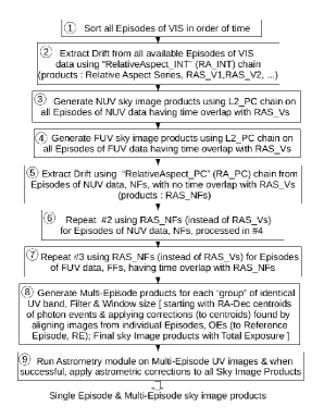
Figure 9: Schematic diagram showing sequence of steps of Driver Scheme (Default case) which operates autonomously on the entire dataset for a specific ObsID (mL1; consists of many Episodes) and generates all requisite products in one go. An Episode represents the dataset from a single imaging session whereas collection of all imaging sessions during that particular pointing of the spacecraft to the target constitutes an ObsID. The two processing chains (each operating for a single Episode at a time), viz., Relative Aspect (RA_INT /RA_PC) and Sky Imaging (L2_PC) are used repeatatively. The former derives the spacecraft drift relative to a chosen reference direction. The latter generates UV images from detected photons after applying corrections for drift and instrument systematics. The Relative Aspect chain, RA_INT, uses VIS data and in its absence, the RA_PC version for NUV/ FUV data. Sky Image Products (UV, Uncertainty & Exposure arrays) corresponding to multiple Episodes with identical filter & window size are generated by combining data from individual Episodes.

Default configuration :

1) Identification of time ordered sequence of available Episodes of VIS band data (say, V1, V2, … Vn).

2) Running of Relative Aspect chain for Integration mode, RA_INT, using VIS band for tracking on each of these individual Episodes to generate corresponding drift series (RAS_V, Relative Aspect Series from VIS). Label these drift series as RAS_V1, RAS_V2, … RAS_Vn and the corresponding time ranges to be TR1, TR2, …. TRn. All these RAS_V products are available in individual sub-directories corresponding to each Episode, inside the directory “/uvit” (see Appendix-10).

3) Identification of data sets for individual Episodes of NUV band and any combination of Filter & Window size (N1, N2, …. Np), which have time overlap with any of the time ranges (TRi : i=1,2, …n) for which RAS_Vs are available from the previous step. Running of Sky Imaging chain L2_PC on each of these ‘p’ Episodes of NUV data. Flagging of the remaining Episodes of NUV band data (if any) which do not have time overlap with any of the time ranges (TRi : i=1,2, …n), and label them as NF1, NF2, … NFm. Products for individual Episodes are stored under unique directories (“/_NUV_1” etc; Appendix-10).

4) Similar to previous step #2 but for FUV band data. Identification of individual Episodes of FUV band and any combination of Filter & Window size (F1, F2, …. Fq), which have time overlap with any of the time ranges (TRi : i=1,2, …n) for which RAS_Vs are available from the step #1. Running of Sky Imaging chain L2_PC on these ‘q’ Episodes of FUV data. Flagging of the remaining Episodes of FUV band data (if any) which do not have time overlap with any of the time ranges (TRi : i=1,2, …n), and label them as FF1, FF2, … FFk. Products for individual Episodes are stored under unique directories (“/_FUV_1” etc; Appendix-10).

5) Execution of Relative Aspect chain for Photon Counting mode, RA_PC, using NUV band for tracking on each of the flagged Episodes of NUV band data NF1, NF2, … NFm (identified in step #2) to generate corresponding drift series RAS_NF1, RAS_NF2, … RAS_NFm. Label the corresponding time ranges of these RAS_NFs to be TR_NF1, TR_NF2, …. TR_NFm. All these RAS_NF products are available in individual sub-directories corresponding to each Episode, inside the directory “/_RAPC” (see Appendix-10).

6) Execution of Sky Imaging chain L2_PC on each of the flagged Episodes (total ‘m’) of NUV band data NF1, NF2, … using the corresponding drift series RAS_NF1, RAS_NF2, … (generated in step #4). Products from this step are stored in additional directories in continuation with those generated at the step #2 above.

7) Execution of Sky Imaging chain L2_PC on those flagged Episodes of FUV band data among FF1, FF2, … FFk, which have time overlap with any of the time ranges TR_NF1, TR_NF2, …. TR_NFm using the drift series generated using NUV data in step #4, viz., RAS_NF1, RAS_NF2, … RAS_NFm. Products from this step are stored in additional directories in continuation with those generated at the step #3 above.

8) After the executions of the Sky Imaging chain has been completed for all Episodes (completing all the 7 steps described above), their products are segregated for identical combinations of the 3 key parameters, viz., UV band, filter & window size, into “group”-s. A process attempts to combine all images in RA-Dec (ICRS) system from individual Episodes (with no subdivision into pseudo-Episodes) belonging to a particular group using the following steps : (i) Identify the Reference Episode, RE, with largest sky exposure, EXP_TIME; (ii) Order the remaining ‘Other Episode’-s (OE_1, OE_2, … OE_n) in descending order of EXP_TIME; (iii) Attempt to match brightest stars (avoiding outer annular region with sky exposure $<$ 20% of peak) from RE with brightest stars from other orbits (OE_1, OE_2, …) one by one. Let ‘k’ cases be successful (k $\leq$ n); (iv) Centroid coordinates of individual bright stars are used to determine relative Shifts & Rotation between each pair of (RE & OE_j; j : 1, 2, … k); (v) Application of identical shifts & rotation corrections to the centroids of to all photon events of the particular individual Episode (“OE_j”); (vi) Application of shifts & rotation corrections to the corresponding Exposure arrays, which involve transformation of individual sub-pixels at 9600$\times$9600 level and re-gridding. Generation of a combined Exposure array by stacking all ‘k’ components; (vii) Populating photon events into ‘aligned_to_RE’ arrays and convertion to combined Signal array (“count / second”) by pixel by pixel arithmetic operations including corresponding aligned and combined Exposure array; One important caveat deserves mention here : while the Exposure arrays from individual Episodes carry the 10% cut, the table of photons which populate ‘aligned_to_RE’ arrays do not. This leads to significantly erroneous values for Signal at the outer regions. For accurate photometry of stars /targets in such affected outer regions the three arrays, i.e. Signal array, Exposure array and Uncertainty array, from each Episode should be added with the shifts and rotations as applicable. (viii) Generation of the combined Uncertainty array. All products resulting from combining of multiple Episodes record in their headers a log identifying the Episode selected as RE, complete list of all the OE-s as well as the Episodes which contributed to these multi-Episode products. It is noteworthy that the final combined multi-Episode UV image (Signal array) is generated directly from transformed centroids of individual photons, just like for individual Episodes, thereby retaining their angular precision despite undergoing alignment operations involving rotation. However, the generation of Exposure and Uncertainty arrays do face some loss of precision, even though their impact is significantly reduced by employing pixel sub-division as described above. The process of combining observations from multiple Episodes includes a check on the difference in the Roll angle values (which is a slowly varying function of time) between the Reference Episode & each of the Other Episodes in order to mitigate their occasional incorrect entries for attitude noticed in the L1 data. This difference is required to be less than 2 degrees for the Episode to be considered for the combining step.

Products generated by this step, corresponding to individual “group” of multi-Episodes are stored under a directory name uniquely identifying that “group” (e.g. “/NUV_Final_F1_W511”; Appendix-10).

9) Execution of Astrometry Module to determine finer corrections & apply them, to the sky coordinates of the multi-Episode combined image products (Signal, Exposure & Uncertainty arrays) for each “group” generated in the previous step. Astrometric corrections are determined by correlating stars identified from the Signal array with standard astronomical catalogues of stars. If successful, identical corrections (involving shifts and rotation of arrays through pixel sub-division, transformation & binning scheme) are applied to each of the set of 3 arrays. For more technical details about this Astrometry Module see Appendix-1 (Sec. A1.20). Products generated by this final step for astrometry, for every “group” of multi-Episodes are stored under an unique directory (e.g. “/NUV_FullFrameAst_F1_W511”; Appendix-10).

Forced NUV tracking configuration :

There is an additional option in the Driver Scheme to completely ignore the VIS datasets & use only NUV data for generating the drift series (RAS) & then make UV images of the sky (both NUV & FUV). In absence of NUV data, the FUV itself can also be used to generate RAS followed by making FUV images of the sky. The Fig. 10 shows possible cases arising due to different kinds of time overlaps between VIS & UV band Level-1 data. Normal situation as per observation planning is case ‘A’, which is ideal and handled using VIS data for tracking. However, sometimes other cases with partial (‘B’ / ‘C’) or no overlap (‘D’) are also noticed which occur due to details of data flow up to the generation of Level-1 data. While the ‘default’ setting of the Driver Scheme (tracking by VIS when any amount of time overlap exists, & force UV tracking when none exists) handles the cases A & D optimally, the remaining cases (B & C) lead to sub-optimal usage of data (limited the overlap part only). This is mitigated by forcing drift tracking with UV data on all the data (ignoring VIS completely). Of course, success with UV tracking critically depends on existence of at least one UV bright star within the field of view. Accordingly, the strategy followed at the UVIT-POC is to execute the Driver Scheme twice, once each with the two options (default & forced NUV tracking) and provide two sets of Level-2 products generated by them, allowing users the choice.

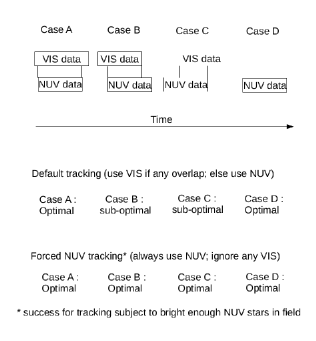
Figure 10: The extraction of spacecraft Drift using VIS & NUV data under different situations of time overlap between sky exposures of VIS and NUV bands. The logic used under “Default” settings of the Driver Scheme, viz., use VIS when any time overlap with UV imaging exists, leads to sub-optimal results for Cases ‘B’ & ‘C’. This is avoided with “forced” NUV tracking. Accordingly, pipeline products generated using both these strategies are provided for the users (when NUV data are available).

3.2.5 Strategy for missing data

In the design of the pipeline, special emphasis has been given to incorporate graceful degradation in view of occasional loss of data at various stages of communication between UVIT and ground station as well as errors encountered in the input products from Level-1. For example – (a) in case of incomplete extraction of drift (e.g. due to large chunk of missing data), images are generated using products for whatever duration they could be salvaged); (b) in complete absence of VIS data for any Episode, the drift extraction is automatically attempted using the NUV data itself; (c) the scheme for combining multiple Episodes, employs a logic which leads to best possible outcomes in the event of sub-optimal signal to noise situation; (d) crash situations of individual processes / chains do not hamper the pipeline from full exploration of the entire data set. The pipeline attempts to maximize the sky exposure translating to scientifically useful products in spite of the limitations in the input data and artifacts therein. The pipeline has been implemented primarily in C++ with total $\sim$ 30,000 lines of code.

3.2.6 Handling special situation

An Episode of observation has been defined earlier as an uninterrupted period of data collection. The input Level-1 science data for an Episode consisting of time sequence of image frames however often show multiple types of anomalies – e.g. missing part / full frames, discontinuities in frame number, frame time & other artifacts. Most such issues have been addressed by gradually improved algorithms incorporated in the Data Ingest block of the pipeline during early in orbit Performance Verification phase of ASTROSAT & UVIT (see Appendix-1, Sec. A1.1 for details). The term pseudo-Episode has also been introduced as the user chooses to divide the data from a normal Episode into multiple parts, Comb_frames (N_combine frames each), to technically address possible misalignments at shorter time scales. For example, when the temporal evolution of spacecraft drift in a particular Episode includes discrete large and fast drifts components, division into pseudo-Episodes is useful. Another example of forced use of pseudo-Episode due to a different reason follows. Under some specific situation arising out of design of UVIT hardware as well as software preceding the pipeline, even a single uninterrupted data collection needs to be sub-divided into smaller pseudo-Episodes (for example : 16-bit Frame Counter overflow in $\sim$ 100 s, during PC mode imaging with the smallest window size 100$\times$100), each holding consecutive 2¹⁶ frames. The last pseudo-Episode would in general contain a smaller number of frames. The pipeline treats each pseudo-Episode at par with a normal Episode.

3.2.7 Modules

The pipeline has been implemented in a modular fashion keeping in mind several blocks of processing are common to different chains and their versions based on imaging mode. Accordingly these are implemented as stand alone Modules for flexibility of being called by different chains. Whenever relevant, these Modules internally support both the imaging modes, viz., Integration (INT) & Photon Counting (PC). Many of them can be turned ON or OFF depending on the user need and / or enabling testing, diagnosing and evaluation. The resulting products from each Module follow a naming convention with name suffix embedded in them. A master list of all the Modules, their functionality and linkages to different chains are presented in Table 3. The large number of selectable switches and variable parameters used by these Modules are provided in Appendix-11. Some generic comments on Modules follow prior to their description. Every Module has several primitive switches regarding overwriting of existing file structure (‘clobber’), inclusion of complete log of operations on product headers (‘history’), choice for timing reference - using the Universal Time Clock or UVIT’s Master Clock (‘utcFlag’), storing outputs from individual block (‘Write_to disk’ flags), etc. The headers of every product from individual Modules record settings of all selectable switches and parameters. In addition, values of various corrections factors (e.g. events rejected due to parity error, CRC, etc), frames affected by Cosmic Ray showers & discarded, frames affected by artifacts in data, initial frames affected by mandatory safety checks which are discarded, etc. are logged in the headers. Every failure to achieve convergence or successful completion of any block is recorded in a master log with a message (including the text string “CRASH”) which helps to track it and relevant details for its later investigation and diagnosis. Individual Modules are described with full technical details in Appendix-1. They are presented in an order following their sequence of appearance in the chains for drift extraction – Relative Aspect (RA_INT & RA_PC; section 3.1.4.1) followed by the Modules exclusively for the chains for Sky Imaging (L2_PC & L2_INT; section 3.1.4.2). In general, within every Chain, almost all Modules process all the frames of an Episode before transferring control to the next Module (only exceptions being the sequence of blocks 10, 11, 12 & 13 in RA_INT chain which form a looping segment; see Fig. 6).

There is also a library of utilities that are commonly used by several Modules & processing blocks.

Table 3: List of Modules used in the Pipeline and their linkages to Chains

Serial	Functionality of the Module	Name of the	References to	Usage
No.		Module	Module description	of the Module
			(Appendix 1)	(Chains)
1	Ingest the observational data	DataIngest	A1.1;	RA_INT, RA_PC,
	as well as calibration databases		Fig.14	L2_PC, L2_INT
2	Unit conversion from ‘event’ to	uvtUnitConversion	A1.2	RA_INT, RA_PC,
	‘event-per-second’			L2_PC, L2_INT
3	Flagging of pixels / events	uvtMaskBadPix	A1.3	RA_INT, RA_PC,
	corresponding to unusable regions of			L2_PC, L2_INT
	the detector
4	Identifying frames affected by	uvtCosmicRayCorr	A1.4	RA_INT, RA_PC,
	Cosmic Ray showers			L2_PC, L2_INT
5	Applying correction for response	uvtFlatFieldCorr	A1.5	RA_INT, RA_PC,
	variation over the detector area			L2_PC, L2_INT
6	Correction for temperature	uvtQEMCPCorr	A1.6	RA_INT, RA_PC,
	dependence of : Quantum Efficiency			L2_PC, L2_INT
	(QE) of detector gain of Micro-
	Channel-Plate (MCP)
7	Symmetric expansion of 2-D arrays to	uvtPixPadding	A1.7	RA_INT, RA_PC,
	accommodate spacecraft drifts			L2_PC, L2_INT
8	Frame Accumulation by stackings	uvtAccEveryTsec	A1.8	RA_INT
	of successive frames
9	Generating finer grid of 2-D arrays to	uvtSubDivision	A1.9	RA_INT, RA_PC,
	achieve / preserve higher resolution			L2_PC, L2_INT
10	Star Detection - identify brighter	uvtDetectStar	A1.10;	RA_INT,
	sources in the sky image		Fig.15	RA_PC
11	Correction for Detector Distortion -	uvtDetectDistCorr	A1.11	RA_INT, RA_PC,
	photon event / star centroids corrected			L2_PC
	for local defects inherent in the
	Detector
12	Correction for Distortion in the	uvtOpticAssDistCorr	A1.12	RA_INT,
	optical assembly - photon event / star			RA_PC, L2_PC
	centroids corrected for local
	distortions in the Telescope optics
13	Identification of a Reference Frame	uvtRefFrameCal	A1.13	RA_INT,
	with respect to which all ‘relative’			RA_PC
	shifts and / or rotations etc are
	computed
14	Computation of drift (for temporal	uvtComputeDrift	A1.14;	RA_INT,
	scale of several seconds) from VIS /		Fig.16	RA_PC
	NUV images to generate Relative
	Aspect Series (RAS)
15	Computation of jitter (for sub-second/	uvtComputeJitter		RA_INT,
	second time scale) from Gyro signals			RA_PC
16	Computation of inter-band alignment	uvtComputeThermal		RA_INT,
	due to thermal effects			RA_PC
17	Correction to the photon event	uvtCentroidCorr	A1.15	L2_PC
	centroids for error in on board
	estimation of dark counts of the
	CMOS sensor
18	Correction for the Fixed Pattern	uvtCentroidBias	A1.16	RA_PC,
	Noise to the photon event centroids			L2_PC
19	Correction for drift by applying Shift	uvtShiftRot	A1.17	L2_PC,
	& Rotation			L2_INT
20	Frame Integration - dividing the full	uvtFrameIntegration	A1.18	RA_PC,
	dataset into smaller sub-sets, as an option			L2_PC
21	Generation of Exposure Weighted	uvtFindWtdMean		L2_INT
	Mean Images & Exposure Arrays
22	Registration & Averaging - aligning	uvtRegAvg	A1.19	L2_PC,
	images from sub-sets of an episode			L2_INT
	and combining into a single image
23	Establishing absolute aspect of the	uvtFullFrameAst	A1.20	L2_PC,
	image by matching catalogued stars			L2_INT,
				Driver Scheme

4 Commissioning experience, operation and performance of the pipeline

Extensive testing of each Module / algorithm as well as the four chains have been carried out over an extended period. This began with data collected in the laboratory in the year 2015, well before the launch of UVIT/ ASTROSAT. The spacecraft drifts were simulated with jigs created to generate relative motion between a UV source and the detector assembly. Most debugging could be completed only after launch with in-orbit data from Performance Verification phase. Some tweaking of strategies and choices of algorithms were also needed. Many of the parameters related to instrument characteristics were refined based on the data from in-orbit calibration, whose starting values were from lab tests. Two noteworthy parameters which needed most careful and laborious analyses are : (i) Relative shifts between time stamps of the frames in the three bands – these are required for translating time-series of the drift derived from one band, e.g. VIS, to the other bands, e.g. NUV and FUV, & (ii) relative angles between the coordinate system (X-Y axes) among the three detectors as well as with respect to the spacecraft coordinates (Yaw-Pitch). A common Master Clock (from the selected band) is used by all the bands for time stamping individual frames. The time offsets between the NUV (or FUV) band (irrespective of window size selection) with respective to the VIS band (as well as between NUV & FUV bands, which is needed in case of drift tracking using NUV) have been calibrated. These are presented in Appendix-2. The details of relative angles between coordinate systems are presented in Appendix-3.

The UL2P described above have been in regular use at the UVIT Payload Operation Centre (POC) for generating standard bundle of products for archiving and dissemination to the community of astronomers by the ISSDC. The UVIT Driver Module is executed twice on each merged Level-1 data set – once using VIS band for drift extraction (RA_INT chain) and the other time forcing the use of NUV band for extracting drift (RA_PC chain). A nominal set of default parameters are used for both the runs. The standard bundle of products for dissemination is selected by the POC & ISSDC, which includes the most important items required by common end users (astronomers). The Table 4 list all contents of this bundle. It includes products for each combination of UV Band, Filter & Window size from individual episode as well as combined over multiple episodes (for details see Appendices 2, 3 & 10). For the single episode case, constituents are : Drift series (RAS; final output of RA_INT/ RA_PC chain; from ‘uvtComputeDrift’ directory; Event list (including final centroids in both Detector & Astronomical coordinates; from ‘uvtShiftRot’ directory; one final post-Astrometry UV sky map (Signal; RA-Dec; ICRS; J2000; from ‘uvtFullFrameAst’ directory), and three pre-Astrometry sky maps of UV (Signal), Exposure & Uncertainty (all in Detector X-Y coordinates; from ‘uvtFlippedRegImage’ directory). For the combined multi-episode case the constituents are : one final post-Astrometry UV sky map (Signal; RA-Dec; ICRS; from the directory like - ‘XUV_FullFrameAst_F1_W511’, where X=F or N for FUV and NUV respectively), and three pre-Astrometry sky maps of UV (Signal), Exposure & Uncertainty (all in Detector X-Y coordinates; from the directory like ‘XUV_Final_F1_W511’). There are two sets of these above constituents – one set each for drift extraction using VIS & NUV. The above is further repeated for each combination of UV Band, Filter & Window size. The complete details of all products (including the standard bundle) from the pipeline are presented in Appendices 2, 3 & 10. The current version (v6.3) of UL2P described here has been in use at the POC since mid 2018. Prior to that, an earlier version (v5.7) was in use.

The UL2P is completely open source and its distribution has been simplified by creating an “Installer” compatible with most Unix operating systems. Relevant instructions for installation and other related information are publicly available for download from multiple sites (https://uvit.iiap.res.in/Downloads;
http://astrosat-ssc.iucaa.in/?q=uvitData;
https://www.tifr.res.in/~uvit/). Two caveats must be noted by users of this pipeline. 1) As has been mentioned earlier (Sections 3.2.3 & 3.2.4) the precision of photometry in multi-Episode UV images for the outmost regions, are compromised by the fact that Exposure arrays from individual Episodes undergo a cut ($<$ 10%) but not the corresponding photons while combining Episodes; 2) The scheme of applying large angle rotation to the Exposure array (e.g. from Detector X-Y system to astronomical RA-Dec coordinate system) leads to small but detectable artifacts of repeated patterns with amplitude $\sim$ few percent. Both these issues have been discovered rather recently and they will be addressed in the next upgrade of the pipeline. The corrective measure for #1 will include applying the exposure based cut ($<$ 10% of peak) on the Signal (unit : count /second) array only (i.e. leaving Exposure & Uncertainty arrays without any cut) at the individual Episode processing level. This will preserve photometric precision of the multi-Episode arrays generated by the Driver Scheme. For the #2, an improved logic for mapping pixels from pre- to post-rotation Exposure arrays will be employed.

Table 4: Standard set of pipeline data products bundled by UVIT POC for dissemination and archiving by the ISRO /ISSDC

Product	Description	Drift	Drift	Drift	Drift	Total
type		extraction	extraction	extraction	extraction	No.
		using VIS	using VIS	using NUV	using NUV	of
		(RAS_VIS)	(RAS_VIS)	(RAS_NUV)*	(RAS_NUV)*	files
		Sky Image	Sky Image	Sky Image	Sky Image
		in NUV band	in FUV band	in NUV band	in FUV band
				*for obsn. till	*for obsn. till
				March 30, 2018	March 30, 2018
Products for each
Individual Episode :
Sky Image	FITS image	1	1	1	1	4
(Detector coordinates; X-Y)	(4800x4800 pixels)
Sky Image, post Astrometry	FITS image	1	1	1	1	4
(Astronomical coordinates;	(4800x4800 pixels)
RA-Dec, ICRS)
Exposure Map	FITS image	1	1	1	1	4
(Detector coordinates; X-Y)	(4800x4800 pixels)
Uncertainty Map	FITS image	1	1	1	1	4
(Detector coordinates; X-Y)	(4800x4800 pixels)
Photon Events List	FITS binary table	1	1	1	1	4
(Photon centroids in both
Detector & Astronomical
coordinates)
Drift Series (RAS file)	FITS binary table	1	1	1	1	2
(In Detector & Spacecraft
coordinates)
Products for each “Group”
of Multi-Episodes :
Sky Image, post Astrometry	FITS image	1	1	1	1	4
(Astronomical coordinates;	(4800x4800 pixels)
RA-Dec, ICRS)
Sky Image, pre Astrometry	FITS image	1	1	1	1	4
(Astronomical coordinates;	(4800x4800 pixels)
RA-Dec, ICRS)
Exposure Map, post	FITS image	1	1	1	1	4
Astrometry (Astronomical	(4800x4800 pixels)
coordinates; RA-Dec, ICRS)
Uncertainty Map, post	FITS image	1	1	1	1	4
Astrometry (Astronomical	(4800x4800 pixels)
coordinates; RA-Dec, ICRS)
Common Products :
Data Quality Report	XML					1
README	TXT					1
ChangeLog	TXT					1
DISCLAIMER	TXT					1
Pipeline Parameter Files	TXT					2

Next, some typical examples of results are presented. Figure 11 displays two typical examples of drifts extracted (along Detector X & Y axes) by the Relative Aspect chain RA_INT using VIS band data. It spans $\sim$ 1200 / 1500 seconds of time. The peak to peak variation of drift is around $\sim$ 160 arc seconds. The sharp spikes (positive in one & negative in another) observed in these plots appear at regular intervals corresponding to systematic jerks imparted by planned mechanical movement of the payload Scanning X-ray Sky Monitor (SSM). The drift extraction process has been able to successfully mitigate any major adverse effect of such rather harsh disturbances on the PSF.

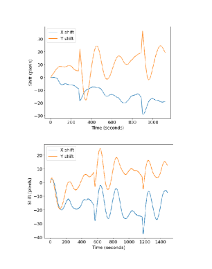
Figure 11: Two examples of drifts extracted by the Relative Aspect chain RA_INT from VIS data spanning 1200 / 1500 sec. The peak to peak movements are $\sim$ 160^′′ (1 pixel $\sim$ 3.3^′′).

Next, as an example we present UV images of an astronomical source, viz., the nearby spiral galaxy NGC 300 at a distance of $\sim$ 1.9 Mpc, processed by the pipeline to demonstrate its efficacy. The Far- UV image is displayed in Fig. 12, which uses 14,300 s exposure with in the filter F148W ($\lambda_{mean}$ = 148.1 nm, $\Delta\lambda$ = 50 nm). The Fig. 13 shows a colour composite Near-UV image of NGC 300 using observations with exposures of 20,000 s in filter N242W (blue; $\lambda_{mean}$ = 241.8 nm, $\Delta\lambda$ = 78.5 nm) & 2,500 s in filter N263M (green; $\lambda_{mean}$ = 263.2 nm, $\Delta\lambda$ = 27.5 nm).

While these sample images show the utility and success of the pipeline in extracting astronomically significant high quality images qualitatively, the POC carries out systematic analyses of the products to quantify their quality objectively. The performance of this Level-2 pipeline has been reported by Ghosh et al. (2021), which had used UVIT observations carried out till mid-2020. Here we have updated it including the latest status.

The FUV and NUV images generated by the pipeline are analyzed for Point Spread Function, PSF, for a minimum of three stars (point sources) spread over the entirefield of view. The extensive in-orbit calibrations have characterized the PSFs for both the FUV and NUV bands by a compact central core and an extended pedestal (Tandon et al 2017c, 2020). Based on these anticipated structure of the PSFs a quality score has been defined. The criteria followed to assign the quality score are : the best score of ‘10’ is assigned if the pedestal is $<$ 20% and the full width at half maxima, FWHM, of the PSF is $<$ 1.6 arc-sec; similarly ‘9’ & ‘8’ correspond to FWHM being $<$ 1.8 arc-sec & $<$ 2.0 arc-sec, respectively. For every increase in the pedestal by 5% (beyond 20%), the quality score is reduces by 2. This score is estimated for both the bands (FUV and NUV) and the mean of these values is quoted in the quality report which always accompanies the UL2P product bundle. The distributions of quality score in FUV & NUV bands for all observations carried out till recently (09-Dec-2021) are shown in Table 5. As can be seen, the pipeline products for NUV band achieve a quality factor of 9 or above for $\sim$ 90% of observations. For the FUV band, this fraction is relatively lower at $\sim$ 54%, which increases to $\sim$ 66% if the quality factor of 8 or above are considered. The relative superiority of the quality score of images in NUV over FUV is related to the fact that the UVIT instrument achieved better angular resolution in the NUV band. Since the NUV band shares the same telescope with VIS band and FUV uses a separate dedicated telescope (see Fig. 2), a possible cause could be temporal changes in the relative angle between the two telescope structures within the time scale of an orbit. Activating the ‘pseudo-Episode’ option for L2_PC chain for the FUV band may improve its quality score.

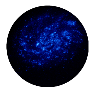
Figure 12: Far-UV image of the Spiral galaxy NGC 300 generated by the pipeline using exposure of 14,300 s with the filter F148W (${\lambda}_{mean}$ = 148.1 nm, ${\Delta\lambda}$ = 50 nm).

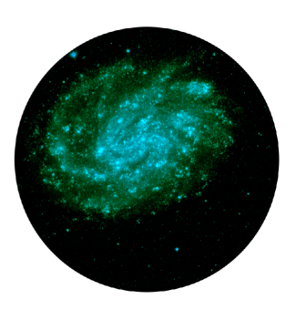
Figure 13: Colour composite NUV image of the Spiral galaxy NGC 300 generated by the pipeline using exposures of 20,000 s in filter N242W (blue; ${\lambda}_{mean}$ = 241.8 nm, ${\Delta\lambda}$ = 78.5 nm) and 2,500 s in filter N263M (green; ${\lambda}_{mean}$ = 263.2 nm, ${\Delta\lambda}$ = 27.5 nm).

One of the key parameters quantifying eventual success rate of the UL2P is the fraction of total on sky exposure finally contributing to the UV image product. The ASTROSAT operations group schedules sky exposures based on approved time allocated (say T_MCAP), for a particular target from a scientific Proposal. Let the Level-1 data successfully generated at the ground station of ISRO be for duration T_L1. This forms the input for the UL2P. Let the final UV image product generated by UL2P be T_L2 (somewhat like EXP_TIME keyword in header). Then yield of UL2P (for that particular episode of observation) can be defined by the ratio - (T_L2 / T_L1). The distribution of this yield for both NUV & FUV observations carried out till recently (09-Dec-2021) are presented in Table 6. The fraction of all pointings in this sample achieving yield above 0.9 (0.8) is $\sim$ 72% (86%) for the NUV band. The corresponding fraction for the FUV band is $\sim$ 75% (88%). These values indicate that there is scope for improvements in the pipeline.

Table 5: Distribution of the quality values (from achieved PSF size & amount of pedestal) for FUV and NUV band images.

Quality bin (range)	(1-2)	(2-3)	(3-4)	(4-5)	(5-6)	(6-7)	(7-8)	(8-9)	(9-10)
NUV band (No. of ObsIDs)	0	0	0	3	6	5	7	18	335
FUV band (No. of ObsIDs)	15	22	30	41	58	84	84	118	527

Table 6: Distribution of the yield values (percentage of input Level-1 data translated to Level-2 image products, for FUV & NUV bands) achieved by the pipeline.

Yield bin (%)	10	20	30	40	50	60	70	80	90	100
NUV band (No. of ObsIDs)	3	0	1	0	7	4	11	27	54	275
FUV band (No. of ObsIDs)	9	5	3	5	9	24	28	72	149	797

5 Summary and possible future improvements

A versatile data processing pipeline (UL2P) has been developed for the UVIT payload on board ASTROSAT satellite. This pipeline runs in a fully automated mode and is ideally suited for the Payload Operation Centre, where huge amounts of data collected from UVIT need to be processed swiftly without human intervention. The pipeline generates astronomer ready sky images in UV. Its main components are : handling of occasional artifacts and anomalies in Level-1 data, extraction of spacecraft drifts, and disturbances due to internal movements; application of various corrections to measured direction of arrival for each photon – e.g. spacecraft motion (with respect to planned inertial pointing towards target direction), systematic effects and artifacts in the optics of the telescopes and detectors, exposure tracking on the sky, alignment of sky products from multi-episode exposures to generate a consolidated set and astrometry. Detailed logs of operations are maintained on headers of products and intermediate products for every processing stage are accessible via user selectable options. This pipeline has been tested extensively before releasing for regular use at the Payload Operation Centre (POC) located at the Indian Institute of Astrophysics (IIA), Bangalore. Every UVIT dataset from ISRO/ISSDC is received by the POC which after processing sends the corresponding standard products back to ISRO/ISSDC for archiving and dissemination. The current version of UL2P described here has been in use since February 2018 and has continued to successfully generate relevant products for the astronomer community leading to scientific results world wide. While large number of selectable parameters are available for the user, a well characterized “standard default” set is used for executing this pipeline at the Payload Operation Centre (POC) for UVIT and selected products are archived and disseminated by the Indian Space Research Organization (ISRO) through its ISSDC portal. Users preferring to use selections of parameters different from the “standard default”, can download, install and run UL2P themselves following instructions provided online. There are a few areas where improvements to this pipeline would help the end users. These include - (1) improvement in efficiency of combining multi-orbit images, (2) improvement in success rate for astrometry correction and (3) improvement in the precision of astrometry. Each of these improvements are linked to use of optical stars (from VIS images) instead of the current scheme of using UV stars detected in UVIT images with significant signal to noise ratio. The scientifically important research areas involving extremely faint fields will benefit most from these.

Appendix-1 : Modules used in the UVIT Level-2 Pipeline

This appendix provides complete technical details of the processing blocks used by the UVIT Level-2 pipeline. Given the two different available modes of imaging operations the processing chains have distinct versions for each of these modes. There are several computational blocks with commonality in their function among the chains / versions. Hence, such processes are captured as Modules with selectable switches and parameters to meet the requirements of all similar applications (see Table 3 for a list of all Modules and their linkages to different chains). A complete list of switches and parameters for these Modules is available in Appendix-11. The Modules are called by the chains and the resulting products from each Module follow a naming convention with name suffix embedded in them for ease of tracking as well as higher level of scripting for autonomous operations. Individual Modules are described next, in a natural order of their sequence of appearance in the chains for drift extraction : Relative Aspect (RA_INT & RA_PC) followed by those exclusively for the Sky Imaging (L2_PC & L2_INT). There are 20 Modules presented below in sub-sections numbered : A1.1, A1.2, … to A1.20. Every Module consists of several blocks operating in a sequence, and in general, each block operates on all the frames of an Episode before transferring control to the next block (with only exception of a few in the RA_INT chain).

A1.1 DataIngest

The Data Ingest is the very first block for any of the processing chains and it prepares all inputs data for processing in the subsequent Modules. Its key functionality is to import input data, check its integrity, sort them into various groups / tables and carry out certain computations. It directly interfaces with the “merged Level-1” (mL1) data bundle which is the primary input to the pipeline, the Calibration Database, CAL_DB, as well as the user selected parameter set (Parameter Interface Library; PIL).

First a brief description of the contents of input data bundle mL1 is presented. The mL1 contains all the Level-1 data products Science Data & Aux Data for the same Observation ID (ObsID; it includes Proposal ID, Target serial number & Pointing sequence number) in an organized manner. Generally the observations corresponding to a specific ObsID lasts multiple successive orbits. The directory structure of a representative data set (mL1) is shown in Appendix-4. The Appendix-5 shows the directory structure of the Calibration Database, CAL_DB. The notation followed to represent multi-level directory structure in Appendix-4 as well as similar other Appendices (5 to 10) is as follows : a normal dash symbol represents files in current directory and a longer horizontal shift or dash represents the next lower sub-directory (followed by the sub-directory name) & the lines immediately following it give contents of that sub-directory. A few files with very long names are broken into two lines with the second line beginning with a large number of dots.

The Science Data are segregated into the three band wise directories. These directories in turn host multiple sub-directories, each of which correspond to one specific “Episode” of data collection. Each sub-directory is populated by 3 files (FITS tables), the imaging data and two files (GTI & BTI) containing flags for a large number of parameters pertaining to the spacecraft & UVIT.

The imaging data are packed as a sequence of “frame”-s, one for each individual exposure, preserving their time order. Each frame comprises of an integral number of fixed size “packets” (2048 bytes) whose contents and format depend on the imaging mode (INT/PC) configured. Each packet begins with the Synchronization Mark, Primary Header and a Secondary Header (includes an Image Frame Counter & various other Counters with timing information) followed by 2016 bytes of image data & ending with a parity-code (CRC). The very first packet of every frame always holds the data for all settings for the Detector Module and the data for system status and health monitoring only. The second packet onwards contains image data. The total number of packets in any frame, $N_{p}$ depends on the imaging mode. The last packet for the frame usually needs padding to complete the stipulated fixed size (2048 bytes). In case of Integration mode (INT), the raw pixel ADUs (2-bytes per pixel) are packed in the usual sequence of 2-D array covering the entire selected window region. Hence, the value of $N_{p}$ is always predictable for INT mode, e.g. maximum value of 262 corresponds to full 512$\times$512 window setting. On the other hand, in Photon Counting mode (PC), the raw pixel signals are processed on board to identify individual photon event and compute its centroid along two detector based axes (X, Y). After this processing, the data from the frame comprises of all extracted photon events packed as a sequence, with each photon event contributing 6 contiguous bytes. Accordingly, each packet can accommodate up to 336 photons. As a result, the value of $N_{p}$ in PC mode may vary from frame to frame, since it depends on the total number of photon events identified. The contents of the 6 bytes for every detected photon event are : centroid along X (2 bytes), centroid along Y (2 bytes), measures of asymmetry in the raw event foot-print & local background (2 bytes).

The Auxiliary (Aux) data correspond to the entire time duration covering the full merged data set. They are FITS tables containing uninterrupted continuous time series of various measured / derived parameters mostly originating in spacecraft sub-systems. Examples of Aux data that are used directly by the pipeline follow. The time correlation between the spacecraft’s clock (raw & calibrated) and internal clocks of UVIT (‘*.tct’). The attitude of the spacecraft : tabulated as quaternions representing rotation angles with respect to reference coordinate system - Roll, Yaw & Pitch (‘*.att’). The signals from the angular rate sensors (Gyros) for the 3 axes (Roll, Yaw & Pitch) which are tabulated separately (‘*.gyr’).

The Fig. 14 provides the sequence of operations carried out by Data Ingest. DataIngest initially carries out the following functions - (i) import mL1 data, (ii) set up structured paths for Science data and AUX data, (iii) establish links to Calibration Database, (iv) import and interpret settings of various user selectable switches and values of parameters, from Parameter Interface Library, PIL, queries.

As a part of check on data integrity at a primitive level, the user selected action is carried out on individual data packets which failed the CRC test. Next, the headers of individual science data blocks corresponding to distinct Episodes are interpreted for various settings : respective observing Band, imaging Mode, Filter, the band selected for Master Clock. For each Episode, a time correlation between UVIT’s Master Clock and the absolute time (Universal Time Clock, UTC, stamped by the Level-1 process) is constructed. Occasionally, the UTC shows erratic behaviour. Even when user selects to use the UVIT clock (i.e. with ‘utcFlag’ switch is OFF), a robust error tolerant scheme has been employed to establish a scheme capable of predicting Modified Julian Date (MJD) from UVIT clock, albeit with limited precision ($\sim$ 1 s).

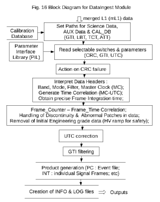
Figure 14: Block Diagram for DataIngest Module. This module first collects all relevant input data from observations, calibration and user selections of configurable parameters. It checks integrity and quality of observational data and separates them bandwise in suitable formats (as per imaging mode : INT / PC) for processing by the later stages. It carries out time correlation and certain other functions as described in the text.

Next step deals with identification and treatment of corrupt and unusable data. The frame number and its corresponding time stamp must always increment in a regular fashion as per the selected parameters related to the frame read-out rate (with the exception of natural return to zero on overflow of the respective counters). This provides a good handle for identifying certain kinds of data corruption. The nature of unusual data patch includes the following occurrences noticed in most Level-1 data sets (in PC mode) : mismatch between Frame Number and Frame Time (one of them being in the correct sequence correct and the other showing a JUMP ‘spike’, which can be positive or negative); completely discontinuous Frame Number & Frame Time inserted within normal good data sequence; data from a particular frame repeated elsewhere in the same data set (i.e. for the same observing Episode); abrupt discontinuity in Frame Number which violates monotonicity, etc. These issues have come to light progressively during the mission and appropriate logic incorporated within this DataIngest Module. As a result this Module has evolved over longer time. The identified ‘outlier’ frames are discarded from further consideration. The fraction of input Level-1 data successfully translated by DataIngest Module to reorganized output usable for the subsequent Modules depends on frequency of occurrences of unusual data patches. Some statistical information based on past $\sim$ 4 years’ operation of UVIT are provided in Section 4.

Initial part of every Episode of observation includes data collected during ramping up of high voltages for detector safety, which is not scientifically useful since the gain is changing with time. These time stretched are identified and discarded. The primary time variable to be used extensively by the subsequent steps of the pipeline is generated by applying UTC correction to UVIT’s Master Clock (only if ‘utcFlag’ is selected to be ON). In case the Good Time Interval (GTI) filtering is turned ON, the time stretches of data not meeting the criteria selected by the user are discarded. The precise value for exposure time per frame is computed and recorded. In actual processing so far, GTI filtering has never been used.

The next phase of processing in DataIngest depends on the imaging Mode. For INT, individual frames containing raw pixel counts are extracted and stored in separate 2-D FITS image files in a directory named ‘SignalFrames’ with nomenclature of each file having Frame number and Time stamp embedded in it. This directory also stores a list of extracted images.

For PC, sequence of individual frames with centroid coordinates in detector X-Y coordinate system and other details like Frame number, UVIT Master clock time, UTC time, diagnostic measures of event’s raw 5x5 pixel footprint - ‘Max-Min’ & ‘Min’ values of the 4 corners for every detected photon are all packed into a single ‘events’ file. It holds the data from the specific imaging Episode as one master list of photon events in chronological order as FITS table.

For both the Modes, the following products are included : UVIT-UTC time correlation table, log of data loss and an ‘info’ file for passing various computed & PIL parameters to the subsequent Modules.

Some long term effects of exposure to radiation (SEE) on the on board electronic components were noticed midway through the mission life. They were recoverable by hardware RESET to the system at periodic intervals. However, some fraction of the data collected were affected beyond the designed immunity in the pipeline. As a result additional software patches were developed and applied at a later stage to mitigate these effects. While nature of these fixes belongs to the DataIngest module, they were accommodated in the envelope code for the chain (RA_INT) and described in Section 3.2.1.

A few general remarks follows, on the convention followed throughout the pipeline for flagging of unusal data / locations. First about flagging pixels /elements of a 2-D image / array, which need not be considered for processing due to either considered as “bad” due to any defect or representing a region outside the active area of the detector. An unique value (-9999) is assigned to such pixels / elements for their easy recognition as an “invalid” pixel / element by all processing blocks. No arithmetic operation is carried out on such flagged pixels / invalid elements & their values are left unaltered. On the other hand, the flagging of individual photons in the master event list are carried out by appending an additional column with an entry with a value ‘1’ (= good) / ‘0’ (=bad) indicating their inclusion / exclusion for consideration in further processing (e.g. event located outside the detector’s active area; asymmetry in footprint signifying multi-photon event).

Directory structures of the products of DataIngest Module for INT and PC modes are provided in Appendix-6 & Appendix-7 respectively.

A1.2 uvtUnitConversion

Aim of this Module, (called by all the versions of the chains) is to translate the image data into physical unit, making it independent of the frame integration time, selected for the observation. For INT mode data, first a dark frame, D(ix,jy), taken from CAL_DB is subtracted from the raw frame, RI(ix, jy), and then divided by the frame integration time, $T_{i}$, (earlier computed by DataIngest Module) making the pixel values to be ‘signal/s’. (The code is designed to derive this dark frame by linear interpolation in time between dark frames taken before the sky-exposure and after the sky- exposure. But, in practice this dark frame is taken from the CAL_DB of ground calibration.) This process is repeated for every image frame.

I_uc(ix,jy)= [RI(ix,jy)-D(ix,jy)]/(T_i);

for all pixels (ix, jy) of the image, & repeated for all images; For PC mode data, each photon event is assigned a value of ‘event/sec’ (1 divided by the frame integration time) and recorded in an additional column of the master table of events. This column is referred to as Effective Number of Photons per second (ENP).

 ENP_uc(k) = [ 1 /(T_i) ];

for all events in master table ‘k’ = 0 to ‘k_max’

Note the suffix ‘uc’ which identifies the outputs with the Module. Similar naming convention is followed for all other Modules also.

A1.3 uvtMaskBadPix

This Module is called by all versions of the processing chains. The functionality of this Module includes identifying and flagging of : (1) bad pixels in INT mode image arrays, & (2) events in PC mode master table with centroids located in bad pixels as well as those satisfying criteria for being classified as multi-photon event. BAD_PIXELS files, for each of the three bands, are arranged as per the mode of observations and the chosen window size, in the CAL_DB. All the inactive pixels, either because of being outside the detector’s circular field of view or beacause of selection of one of the smaller window options, are represented as ‘bad pixels’ by populating ‘0’ entries (rest with ‘1’ entries), in the corresponding BAD_PIXELS file BP(ix, jy). For INT mode the flagging is effected on all bad pixels of each image frame.

 if BP(ix, jy) = 0, then
 I_bp(ix, jy) = INVALID_PIX_VALUE;
 else I_bp(ix, jy) = I_uc(ix, jy);

As stated earlier (Sec A1.1), a value of ‘-9999’ is assigned for the ‘INVALID_PIX_VALUE’ flag. For PC mode, every photon event is assigned a value for the variable ‘BAD_FLAG’ depending on the integral parts of its centroid coordinates. The centroid coordinates, (x, y), are real numbers represented by an integer part (in the range : 0 - 511) and a fractional part. Consider the integer parts of the centroids (x, y) to be (ix, jy). A new column for ‘BAD_FLAG’ is appended to the master table of events, which is populated with :

BAD_FLAG(k) = BP(ix, jy),

where centroid coordinates for the event ‘k’ are (x, y);for all events in master table ‘k’ = 0 to ‘k_max’ This Module carries out another function for the PC mode, viz., flagging for Multi-photon events. The option for discarding events having two neighbouring photons was introduced with the aim of achieving higher angular resolution. On board processing in PC, mode for detecting individual photon events from raw frames, also extract diagnostic information as stated earlier. The identification of a imulti-photon event is based on this diagnostic data, ( ‘Max-Min’ & ‘Min’ among the raw counts from 4 corners of the 5x5 photon event footprint, ) and the selected threshold value, ‘mult_photon_thrsld’. For events meeting the above condition are flagged for potential rejection (= ‘0’) in the ‘MULTI_PHOTON’ column appended in the master table of events.

if [Max-Min](k) > mult_photon_thrsld,
 then MULTI_PHOTON(k) = 0;
else MULTI_PHOTON(k) = 1;

for all events in master list ‘k’ = 0 to ‘k_max’ Subsequent processing has the option to discard every frame with even one event with multi-photon flag set for rejection from further consideration. However, this option has never been used.

A1.4 uvtCosmicRayCorr

This Module handles the effects of Cosmic Rays and is called by all versions of the processing chains. There is a provision for by passing this Module.

This Module attempts to mitigate the effects of individual primary Cosmic Ray (CR) hits as well as shower of secondary charged particles generated by interaction of CR within and near the detector. Some of the charged particles would pass through the CMOS imager leading to a large signal in individual pixels, while other charged particles and photons would generate light pulses some of which look like photon events in the PC mode. In the INT mode, the former can be detected as unusually large signals in individual pixels the latter cannot be isolated as these would be similar to genuine photon events. In the PC mode, some of the hits would generate a large shower of events in a frame which can be distinguished statistically from the normal frames. For INT data, pixels with values above a selected threshold, CR_thrshld, are flagged and the process is applied on all the frames.

 if I_bp(ix, jy) > CR_thrshld, then
   I_cr(ix, jy) = INVALID_PIX_VALUE;
 else I_cr(ix, jy) = I_bp(ix, jy);

for all pixels (ix, jy) of the frame.

For PC mode data, CR affected frames are first identified based on their event count being larger than a dynamically determined ‘event_count_threshold’ and then flagged. All events from these flagged frames are ignored for further processing. The value of ‘event_count_threshold’ is computed using two user selected parameters (p & q) as follows :

$$event\_count\_threshold=$$

$$AVG+p*(AVG)^{0.5}+q/((AVG)^{0.5})$$

where, AVG is an estimate for the average number of true photon events per frame determined from the entire data set for that observation episode. The statistical scheme employed for finding AVG iteratively removes the CR affected frames from the sample as “outliers”. The second term in the equation addresses fluctuations in case of very low values of event counts encountered for fields very dark in the UV. At first the CR affected frames are identified using their unique frame numbers and then all photon events from those CR affected frames are removed from the master list of events (& separately recorded in the log of CR affected frames). As a result, the total number of useful frames is reduced. The loss would depend on the orbit and distribution of matter in the spacecraft, and for UVIT it is $\sim$ 5 frames/s. Therefore, for optimal results this correction is only useful for dark fields where contribution of the Cosmic Rays to the photon counts is not much less than the contribution of the background.

A1.5 uvtFlatFieldCorr

This Module, called by all the versions of the chains, applies a multiplicative correction for variations of response of the detector and transmission of the selected filter across the field. The correction factor arrays are available from the CAL_DB (FLAT_FIELDS_FILTER). The array appropriate for the band, mode and filter is selected to apply this correction. For INT mode this 2-D correction array, FF(ix, jy), is multiplied to every image frame, leaving flagged pixels (flagging process assigned an unique ‘invalid’ value for its easy identification) unaltered.

 if I_cr(ix,jy)=INVALID_PIX_VALUE, then
  I_ff(ix,jy) = INVALID_PIX_VALUE;
 else I_ff(ix,jy)=I_cr(ix,jy)*FF(ix,jy);

for all pixels (ix, jy) of the frame.

In case of PC mode data, the value in ENP column for each event is replaced after multiplying it with the correction value from the array element corresponding to that event’s centroid coordinates.

 ENP_ff(k :ix,jy)= ENP_uc(k)*FF(ix,jy);

where integer part of the centroid coordinates of the event ‘k’ are (ix, jy); for all events in master list ‘k’ = 0 to ‘l_max’

A1.6 uvtQEMCPCorr

This Module corrects for the thermal effects on the detector’s response - through variation of Quantum Efficiency and gain of the Micro_Channel_Plate assembly. This Module is called by all the versions of the chains and it can be turned off. It uses Aux (LBT) data for reading the instantaneous temperature of the detector Module (Camera Proximity Unit, CPU) and estimates corresponding multiplicative correction factor by interpolating the relevant table from CAL_DB (QE_TEMP). The in orbit thermal stability of the CPUs have been so good that so far this correction was never required.

A1.7 uvtPixPadding

This Module is called by all versions of the processing chains. In order to accommodate movements of the UVIT field on sky due to spacecraft drift over the duration of Episode, it is necessary to enlarge the size of the 2-D arrays representing the sky images. For INT mode all image frames are expanded from 512$\times$512 to 600$\times$600 size, I_pp(ix, jy), by introducing a 44 pixel wide boundary on all four sides and assigning each of these added pixels with the value of ‘Bad Pixel’ flag. For the PC mode data, centroid coordinates (cx, cy) for all photon events are incremented by (+44, +44) along both axes :

cx_pp= cx + 44; & cy_pp= cy + 44;

for all events in master list ‘k’ = 0 to ‘l_max’. It may be noted that the size of the padding chosen leads to a natural limitation of inclusion of the sky exposure data corresponding to spacecraft drifts at one go. However, a data set with unusually large total drift can still be handled by sub-dividing it into multiple (non-overlapping) time ranges chosen intelligently based on the drift profiles along the two axes (X, Y). Its implementation involves selections of parameters for the Module uvtRefFrameCal described later on (see Sec. A1.13). The pipeline will then need to be executed as many times as the number of sub-divided datasets.

A1.8 uvtAccEveryTsec

This Module is called only by the Relative Aspect chain for Integration mode data (RA_INT). Functionality of this Module is to accumulate selected number, ‘N_acc’, of successive INT mode frames to enhance the signal for detection of faint stars with a good S/N ratio. A pixel by pixel averaging is carried out resulting in accumulated frames, Acc_frame-s. This Module does not handle PC mode (instead this functionality is embedded within the RA_PC chain directly).

A1.9 uvtSubDivision

This Module is called by all versions of the processing chains, with the functionality of dividing the image pixels or their coordinates in to sub-pixels.

The target angular resolution for UV bands of UVIT was $<$ 1.8^′′, while the pixel scale for the final 512$\times$512 CMOS sensor is $\sim$ 3.3^′′. The detector system and on board processing for PC mode ensures precision of determining event centroid coordinates (X, Y) to 1/32 of each pixel ($\sim$ 0.1^′′). As a result, there is a need for sub-dividing various arrays. A subdivision by 8x8 has been used to get more than 4 effective pixels within the required resolution (i.e. mapping 600$\times$600 to 4800$\times$4800). For PC mode, photon event centroids :

cx_sd= cx_pp*8; & cy_sd= cy_pp*8;

for all events in master list ‘k’ = 0 to ‘l_max’.

For INT mode processing, an user selectable factor, sub_div_factor, m (= 2 / 4 / 8) has been introduced for sub-division. This Module implements this sub-division where, original contents of the individual pixels are equally divided among the corresponding sub-divided pixels depending on value of sub_div_factor, m. The sub-pixels corresponding to flagged pixels are retained as flagged.

if I_acc(ix, jy) = INVALID_PIX_VALUE, then
   I_sd(i_m_x, j_m_y) = INVALID_PIX_VALUE;
else I_sd(i_m_x,j_m_y)=I_acc(ix,jy)/(m^2);

over (m x m) sub-pixels;

for all pixels (ix, jy) of the image, & repeated for all the images;

A1.10 uvtDetectStar

This Module is for identifying stars in an image and quantifying coordinates of their geometric centroids. It is called by all versions of the chains.

This Module processes individual sky images to identify candidate stars from local maxima in light distribution, confirm them to be stars from refined analyses of neighbourhood pixels and compute the centroid coordinates. Finally an intensity ordered table of stars is generated. This Module supports both INT and PC mode data. The functionality of this Module is very basic & general purpose, accordinglyit is called explicitly by the two chains extracting spacecraft aspect (RA_INT & RA_PC) and implicitly by the remaining two chains for their larger Modules : uvtRegAvg (Sec. A1.19), uvtFullFrameAst (Sec. A1.20), which are described later. Fig. 15 presents a schematic flowchart for this Module. In brief, the implementation is as follows. The values of all valid pixels in the input sky image frame are used to determine the ‘mean (MN)’ & ‘standard deviation (SD)’ for the background, after removing ‘outliers’ (due to presence of stars) by using an iterative scheme. An initial starting ‘threshold’ for detecting a star is defined as (MN + p * SD), where ‘p’ is user selectable and is initially kept at a conservatively high value ($\sim$ 10 - 50). At first all pixels with values above this threshold are considered to be associated with potential stars. If their number is lower than the user selected value for minimum number of stars, ‘min_stars’, then the value of ‘p’ is reduced gradually and the process repeated, till the requirement is met.

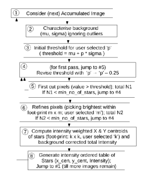
Figure 15: Flow chart for star detection (uvtDetectStar module). The algorithm for detecting stars is based on identifying local peaks above a threshold which is sum of average background and the standard deviation multiplied by a factor, ‘p’. The value of ‘p’ is tweaked iteratively (initially starting with a high value) till the desired number of stars are identified. Centroid positions and intensity for the stars are tabulated.

Multiple neighbouring pixels at this stage could correspond to the same star. In the next step, a neighbourhood criterion using a square box foot print for the star image is used to identify the brightest pixel in each box to get a refined list of pixels (rp_ix, rp_jy). Size of the box is user selectable but the optimal size is found to be 15x15. Whether the candidate mimics signatures of a genuine star is tested by an elaborate logic using the values of the neighbouring pixels, thus providing immunity against noise spikes. If the number in this refined list does not meet the ‘min_stars’ condition, then the value of ‘p’ is reduced further and both the steps described above are repeated till the condition is met (or ‘p’ reaches a value $<$ 5 & the process aborts with appropriate error log).

In the final step, intensity weighted centroid and background corrected total intensity in the box are computed. They are computed as :

c_l_x=[sum{sig(ix,jy)*ix}/sum{sig(ix,jy)}]
c_l_y=[sum{sig(ix,jy)*jy}/sum{sig(ix,jy)}]
  int_l = [sum{sig(ix,jy)}]

where sum is evaluated for ‘ix’ & ‘jy’ running through [rp_ix – (k+1)/2] to [rp_ix + (k+1)/2] & [rp_jy – (k+1)/2] to [rp_jy + (k+1)/2], respectively , where ‘k+2’ is size of the box and ‘sig’ are background corrected values of signal.

Finally, an intensity ordered (descending) table of intensities (int_l) and centroids (c_l_x, c_l_y) is generated.

A1.11 uvtDetectDistCorr

This Module is called by both INT & PC versions of the Relative Aspect chain and the PC version of the Sky Imaging chain.

This Module applies corrections for the distortion inherent to the detector Module (primarily due to the fibre optic taper). This distortion modifies the expected linear relation between location of electronic detection of a photon event and its original location of arrival on the photo-cathode. Hence, in order to determine the true position for each photon event, a correction needs to be applied. This correction has been quantified by extensive calibrations in the laboratory and confirmed in orbit using well studied astronomical targets. The corrections are identical for all the filters of the band and are available in the CAL_DB (DISTORTION/ DETECTOR/ band) as 512$\times$512 arrays. For PC mode, the correction is applied to centroids of every individual photon event & for INT mode to the centroids of each detected star tabulated by the uvtDetectStar Module (Sec. A1.10). The correction values applicable to the nearest pixel coordinates for each centroid (c_x, c_y) are applied :

c_x_ddc = c_x -
det_dist_corr_x{nint(c_x-44),nint(c_y-44)};
c_y_ddc = c_y -
det_dist_corr_y{nint(c_x-44),nint(c_y-44)}

where the arrays ‘det_dist_corr_x’ & ‘det_dist_corr_y’ are from CAL_DB (for appropriate band FUV / NUV / VIS). An offset in indexing (by 44; see Sec A1.7) is needed since the arrays in CAL_DB are in 512$\times$512 system (& all coordinates subsequent to uvtPixPadding Module have them translated to 600x600 system to accommodate spacecraft drift).

A1.12 uvtOpticAssDistCorr

This Module is called by both INT & PC versions of the Relative Aspect chain and the PC version of the Sky Imaging chain.

This Module corrects for distortion due to the Telescope Optical Assembly and is very similar to that discussed above (uvtDetectDistCorr in Sec. A1.11). This distortion has been estimated from design of the telescope and is very small. The corrections to be applied are available in the CAL_DB (DISTORTION /OPTICS /band/filter). It may be noted that since this particular correction originates from design of the telescope optics alone, the CAL_DB arrays are identical for all filter-band combinations. For PC mode, the correction is applied to centroids of every individual photon event & for INT mode to the centroids of each detected star tabulated by the uvtDetectStar Module (Sec. A1.10). The correction values applicable to the nearest pixel coordinates for each centroid (from the earlier Module, say, c_x_ddc, c_y_ddc) are applied :

c_x_oadc = c_x_ddc -
 optic_assm_dist_corr_x{nint(c_x_ddc-44),
                      nint(c_y_ddc-44)};
c_y_oadc = c_y_ddc -
 optic_assm_dist_corr_y{nint(c_x_ddc-44),
                      nint(c_y_ddc-44)}

where the arrays ‘optic_assm_dist_corr_x’ &
‘optic_assm_dist_corr_y’ are from CAL_DB (for appropriate band FUV / NUV / VIS & filter F1/ F2 / …) in 512$\times$512 system.

A1.13 uvtRefFrameCal

This Module selects timing reference and step size for subsequent extraction of drift series. It is called by both INT & PC versions of the Relative Aspect chain. This Module is responsible for two functionalities : (1) generate the Reference Frame defined by an ensemble of centroids and intensities of the detected stars with respect to which all relative aspects for future instances of time will be computed, & (2) to prepare tables, similar to the preceding “(1)”, of detected stars for all subsequent time samples. These are then used to find the drifts in a later processing Module (uvtComputeDrift in Sec. A1.14). It begins with the tabulated lists of distortion corrected centroids of stars detected. Each table represents one time sample. The sequence tables as a time series have been generated earlier from individual Acc_frame-s (by uvtDetectStar in Sec. A1.10). There are two user selected parameters for this Module, viz., number of initial time samples to be ignored, N_skip, & the number of successive time samples to be combined as a block, N_avg, to effectively widen the time bin for computing the average positions of the stars. The resulting time series from the sequence of blocks will subsequently be used for computation of the drift. The very first block is used to generate the Reference Frame by associating stars using neighbourhood criteria on the centroids from N_avg number of individual Acc_frame-s. This is followed by recording the average values for centroid along X, centroid along Y, Intensity & Time. This process is repeated for the subsequent blocks. The selectable parameter N_skip provides a scheme to handle data set withunusually large drift, by breaking down the full time range into multiple parts.

A1.14 uvtComputeDrift

This Module is called by both INT & PC versions of the Relative Aspect chain. It supports both INT & PC mode input data and carries out the following tasks : (1) compute the drift which includes shifts and rotation of the field of selected UVIT band as a function of time in Detector coordinate system to generate Relative Aspect Series (RAS); (2) time domain digital low pass filtering of the RAS using selectable parameters; & (3) to translate the filtered RAS to the spacecraft coordinate system, viz., Roll, Yaw & Pitch using mechanical and optical mounting details of the bands on the spacecraft. The Fig. 16 presents the schematic flow of processing in this uvtComputeDrift Module.

The drift computation involves at first reading in all the tables of centroids & intensities for stars, from products of the earlier Module uvtRefFrameCal (Sec. A1.13). In the next step, within a loop, two consecutive tables are considered which are referred to using subscripts ‘p’ & ‘c’ for ‘previous’ and ‘current’ respectively. The stars common to both the tables are identified and associated as pairs using their centroid coordinates and an user selected neighbourhood criterion representing maximum expected relative drift.

The generation of the RAS involves computation of best estimates the three variables ‘$\delta$x_shift’, ‘$\delta$y_shift’ & ‘$\delta\theta$’ in detector coordinate system, representing the best fit for transformation of centroids from ‘table_p’ to ‘table_c’. This best estimation is carried out using the centroids and a selectable algorithm (3 choices available). The most commonly used algorithm finds solution for least sum of squares of deviations, while giving equal weight to all the stars to avoid bias due to some bright stars in few locations. The algorithm is linearised by use of the approximation “sin $\delta\theta$ = $\delta\theta$ and cos $\delta\theta$ =1” which is valid as the relative rotations within any Episode are $<$ 0.1 degree.

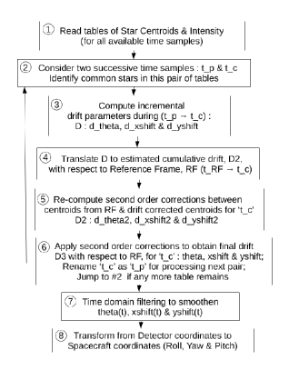
Figure 16: Flow chart for extraction of drift (uvtComputeDrift module). Using centroids of detected stars in successive frames (sampled every $\sim$ 1 sec for VIS tracking) the incremental relative drift local in time is estimated first. The quantified drift includes 2 shifts along the detector axes and a possible rotation. Subsequently they are translated to cumulative total drift as a function of time, with respect to the Reference Frame. Time domain filtering is used for smoothen the 3 drift variables. Finally they are transformed to spacecraft coordinate system (for use by any of the bands).

In order to limit the error propagation through addition of multiple incremental corrections over multiple time steps, the above scheme is repeated again between the star centroids in the Reference Frame (time_RF) and the drift corrected centroids for any time sample time_c obtained above. The additional corrections obtained now (say, $\delta\theta$2, $\delta$x2_shift & $\delta$y2_shift) are used to compute the final drift values valid for time_c, as :

$\theta$_RF_fin(time_c) = $\theta$_RF_est(time_c) + $\delta$$\theta$2
x_shift_RF_fin(time_c) = x_shift_RF_est(time_c) + $\delta$x2_shift
y_shift_RF_fin(time_c) = y_shift_RF_est(time_c) + $\delta$y2_shift

The complete process described above is repeated for the entire time range by advancing the time by steps of one in a loop. The resulting time series of $\theta$_RF_fin, x_shift_RF_fin & y_shift_RF_fin are the Relative Aspect Series in Detector coordinate system. Other choices of algorithm for extraction of drift parameters include : (a) dropping the assumption about ‘$\theta$’ to be small; & (b) assigning intensity based weights to individual stars (weight proportional to intensity). In all the 3 algorithms, user has a choice to drop the parameter ‘$\theta$’ from drift extraction (i.e. consider only shifts and no rotation).

The time domain low pass filtering is carried out to minimise errors in the drift parameters . A sliding time window ($\Delta$T) selects the samples over (t- $\Delta$T/2) to (t + $\Delta$T/2) duration. They are then fitted with a polynomial of degree ‘n_poly’ using a least square method. The value for fittedpolynomial at mid-point of the time window is assigned as the filtered result for time instance ‘t’. This process is repeated through the complete time series. While $\Delta$T and n_poly are selectable by the user the most commonly used values for these have been 4 seconds & 1 respectively.

Finally the drift parameters are transformed from the Detector coordinate system to the spacecraft coordinate system using available transformation matrices. The convention followed for mapping them are : $\theta{\Rightarrow}$ Roll, X $\Rightarrow$ Pitch & Y $\Rightarrow$ Yaw. Details of the two way transformations between the Detector and spacecraft coordinate systems are available in Appendix-3. The final Relative Aspect Series, RAS, are made available in both the detector as well as spacecraft coordinate systems, which are required by both versions of the Sky Imaging chains (L2_PC & L2_INT). The standard bundle of the pipeline products includes the two RAS tables for every individual Episode, one each from RA_INT and RA_PC chains. The tables show the drifts at regular intervals of time.

A1.15 uvtCentroidCorr

This Module was planned for the PC mode version of the Sky Imaging chain. It corrects for a subtle effect which introduces shift in the centroid of a photon event computed on board. It can arise if estimate of the background signal, which is equated to the lowest value of the four corner signals of 5X5 window around centre of the event, used for on-board calculations of centroid differs significantly from the actual value due to a large noise. The mitigation scheme employed use of median filtered background from measured dark frames in orbit. During early operations in orbit, the noise in background was found to be insignificant. Accordingly, need for activating this Module has not arisen. This correction must precede the correction for centroid bias (uvtCentroidBias, Sec. A1.16) described next.

A1.16 uvtCentroidBias

This Module is called by both the Relative Aspect & Sky Imaging chains for the PC mode. It applies corrections for bias introduced on the centroids of photon events computed by on board signal processing. This systematic bias is inherent to the scheme adopted for obtaining the centroids from raw pixel values in the event foot print (3x3 or 5x5), which slightly modifies the fractional part of the computed centroid value from the corresponding true value. Sometimes this effect is also referred to as Fixed Pattern Noise. The effects of this bias have been quantified from the extensive laboratory calibrations which have been translated into look up tables correlating the measured with the true values for the fractional part of the centroids along both the axes (X, Y). The CAL_DB provides these look up tables. This uvtCentroidBias Module recovers the true value from the measured one by applying the corresponding correction (for the appropriate band FUV / NUV / VIS & selected foot print 3x3 / 5x5; e.g. BIAS_CORR/FUV/3x3) to all centroids in the master table of events.

A1.17 uvtShiftRot module & further updating of event table

This Module is called by both INT & PC versions of the Sky Imaging chain. The uvtShiftRot Module carries out the following two tasks for INT mode observations : (A) apply the drift to individual images - single frame or ‘N_acc’ frames clubbed together as Acc_frame in the Module uvtAccEveryTsec, to align these with the Reference Frame; (B) create Exposure Arrays corresponding to each individual image taking into account the active areas of the detector and aligning them to the Reference Frame by applying drift corrections. For the PC mode, only the first of these two functionalities is incorporated by applying the drift to the centroids of photons. In the PC mode, instead of Exposure Arrays for individual exposure an integrated Exposure Array is created by adding the Exposure Arrays corresponding to individual images. This has been done as the number of individual images in an Episode could be about a million storing these individually would be too expensive in memory space.

A1.17.1 Task-A :

The drift parameters for every image are calculated by a linear interpolation of the entries in the table of drifts for the band, provided by A1.14 uvtComputeDrift, at the relevant time.

A1.17.1a PC mode -

For PC mode data, these interpolated drift parameters are used to apply identical corrections to centroids of all photon events of the specific frame.
c_x_snr= x_shift + (c_x -x0)*cos$\theta$ - (c_y -y0)*sin$\theta$ + x0
c_y_snr= y_shift + (c_x -x0)*sin$\theta$ - (c_y -y0)*cos$\theta$ + y0

where x0 = x_size/2 & y0 = y_size/2; where the ‘snr’ subscript refers to the shift and rotation corrected centroids & the (c_x, c_y) are the most recently updated centroids from the master photon event list from the module “uvtOpticAssDistCorr” (Sec A1.12). These drift corrected centroid values (c_x_snr, c_y_snr) for each photon event replace the earlier entries for centroid values in the master table of events and remain available for subsequent processing blocks till the very end of execution of the chain. In case the RAS does not cover the entire time range for the Episode, only the part with time overlap is retained and the remaining events are discarded since the drift corrections can not be applied to them. This updated table is preserved in the sub-directory labeled ‘uvtShiftRot_6.3’ within the product bundle for the corresponding Episode, in a file named with the suffix ‘_snr’ (see Appendix-9).

Further updating by a later processing (uvtFullFrameAst Module) :

The photon event table finally updated by this uvtShiftRot Module (described above) gets further refined by a later processing Module carrying out astrometric corrections by matching detected stars with those in an existing standard catalogue (module uvtFullFrameAst; Sec. A1.20). A new event table is generated which adds fresh information regarding coordinates and time while retaining all the past details, located in the same sub-directory with the file name having the suffix ‘_radec’.

Five additional columns are appended, which are named ‘RA’, ‘DEC’, ‘MJD_L2’, ‘RA-aaaaa’ & ‘DEC-aaaaa’. The first pair contains the best estimate of the event coordinates in RA, Dec (ICRS; J2000) system relative to the map centre, which are the final values obtained from the pipeline run for the corresponding Episode including Astrometry. The last pair correspond to the RA, Dec obtained through transformation of event centroids from Detector (X, Y) system to RA, Dec system using the aspect information from the spacecraft. In the event of failure of the astrometry block, both sets of coordinates would be identical.

The column named ‘TIME’ was planned to provide the primary timing information for each photon event. It is normally populated with SPS_MJD, the absolute time provided by L1 through calibration of the spacecraft’s on board clock, through selection of the ‘utcFlag’ to be ON. Alternately, if the UTC switch is selected to be OFF (when SPS_MJD showed erratic values occasionally), this ‘TIME’ column is populated with the UVIT’s Master clock, and the ‘MJD_L2’ column in the table would still provide estimated absolute time with about $\sim$ 1 sec accuracy, using local calibration of the UVIT’s Master clock (carried out within the L2 pipeline, in DataIngest Module – Sec. A1.1). This enables astronomical variability analysis at time scales shorter than typical duration of observation episodes which is $\sim$ 2000 seconds under all circumstances.

The standard bundle of the pipeline products disseminated by the ISSDC includes this final resulting table (with suffix ‘_radec’), as the event list table, corresponding to every data set from individual Episodes.

A1.17.1b INT mode -

For INT mode data, individual image frames are first transformed by pixel sub-division from original size 4800$\times$4800 to 9600$\times$9600. Then contents of each of these finer sub-pixels are moved to a new location after application of the shift and rotation correction using relations similar to the above. Finally, a 2x2 binning is carried out to bring the array dimensions back to original level. The process ensures local ‘conservation’ of signals and adequate handling of ‘Bad Pixels’. At the end, as many drift corrected image frame products are generated as were available at the input. They are all in Detector coordinate system (X, Y).

A1.17.2 Task-B :

For the second task of generating Exposure Arrays, at first the relevant “Template Exposure Array” is accessed from CAL_DB (EXPOSURE_TEMPLATE / band / mode / window size). Primarily, entries in this array are ‘1’ for all sub-pixels corresponding to the good pixels within the selected window and ‘0’ for the rest. For every image qualified for inclusion in making sky image, a corresponding Exposure Array is generated by applying drift corrections (on the template array) appropriate for that time instance following the procedure described in Task-A (A1.17.1b INT mode).

A1.18 uvtFrameIntegration

This Module is called by both the Relative Aspect and Sky Imaging chains for PC mode data. It is responsible for gridding the photon centroids from multiple (N_combine) successive frames onto 2-D array/(s). For the RA_PC chain, a time series of images, Comb_frames, are generated which are used for identifying individual stars in a subsequent processing stage. For the L2_PC chain this module is either used to combine all the frames for the Episode into a single image or construct multiple images by sub- dividing the full data into smaller time intervals corresponding to ‘pseudo-Episode’-s. The latter option enables application of corrections for small mis-alignments due to any temporal effects, in a subsequent processing step (module uvtRegAvg; Sec. A1.19).

The typical values of the time step ‘T’ corresponding to the selectable parameter, N_combine, are $\sim$ 1 s and $\sim$ 300 s for RA_PC and L2_PC chains respectively. Time sequence of images, Comb_frames, are referred to as 4800$\times$4800 “Sig” arrays. The last image would be made with $<$ N_combine frames in case the Total number of frames is not integer multiple of N_combine. There is a provision to skip N_discard initial frames to discard the initial frames either due to any starting disturbance or during a rapid drift of the pointing. Corresponding sole / sequence of “Exposure” array/s and “Uncertainty” array/s are also generated in the L2_PC chain. The “Signal” array/s are obtained by pixel by pixel division of the “Sig” array/s by the corresponding “Exposure” array/s and the statistical “Uncertainty” array/s are generated using the “Signal” and “Exposure” array/s (based on square-root of estimated number of total EFFECTIVE photon events, corrected for the variation of responsivity on the detector, in each individual pixel and not the actual number of photon events). The “Exposure” products from this module are stored in the directory ‘uvtExposureFrames_6.3’ and the rest (Sig, Signal & Uncertainty) in sub-directories under the directory ‘uvtFrameIntegration_6.3’.

A1.19 uvtRegAvg

This Module is called by both INT & PC versions of the Sky Imaging chain. It may be noted that in an earlier processing block (PC : uvtFrameIntegration Module; Sec. A1.18; INT : uvtFindWtdMean for L2_INT (not described here), the dataset from a specific Episode has either been treated as a whole (‘Episode’) or in smaller parts (‘pseudo-Episode’) as per user’s choice. Here, the Module uvtRegAvg, combines the multiple Signal (“Sig”) and Exposure (“Exposure”) arrays in case ‘pseudo-Episode’ option was exercised in that earlier bloc. These multiple ‘Sig’ & ‘Exposure’ arrays are combined after determining relative Shifts and Rotation between them using an algorithm to align detected brightest point sources from successive ‘Sig’ arrays which were generated earlier on. The alignment operations are identical for each pair of ‘Sig’ & ‘Exposure’ arrays.

Additionally, for PC mode UV imaging, these combined ‘Sig’ & ‘Exposure’ arrays are used to generate the output ‘Signal’ & ‘Uncertainty’ arrays in true “count/second” unit, using the same scheme as described earlier (uvtFrameIntegration Module; Section A1.18). The same operation is carried out on the sole pair of ‘Sig’ & ‘Exposure’ arrays in case the ‘Episode’ option was exercised in the preceding processing block to generate all 3 final products, viz., ‘Signal’, ‘Exposure’ & ‘Uncertainty’.

At the end of this uvtRegAvg process (irrespective of the choice between pseudo-Episode / Episode), a single set of sky image, exposure & uncertainty products are generated which utilize the entire data set for the particular observation Episode (for a particular combination of Band, Filter & Window size in one orbit). These final array products Signal (counts/sec), Exposure (no of frames) & Uncertainty (counts/sec) are of 4800$\times$4800 size and in Detector coordinate (X, Y) system and stored in the ‘uvtRegAvg_6.3’ directory (see Appendix-9).

Since the algorithms used in this uvtRegAvg Module for 3 different steps of processing are identical to those described earlier for other Modules, only their references are mentioned here. The scheme to find bright point sources in individual component images (from pseudo-Episodes) is similar to that used for the Module uvtDetectStar (Sec. A1.10) & to determine relative offset (shifts and rotation) between them uses the scheme followed for the Module uvtComputeDrift (Sec. A1.14). Finally, the scheme employed for aligning these individual images based on the locations of detected point sources, is the same as followed for the Module uvtShiftRot (Sec. A1.17.1b; Task-A, for INT mode). It may be noted that the alignment of pseudo-Episodes involves transformation of image sub-pixels resulting in some loss of angular precision, unlike alignment among Episodes carried out in the Driver Scheme (Sec. 3.2.4) in which individual photon centroids are transformed.

A1.20 uvtFullFrameAst

This Module is called by both INT & PC versions of the Sky Imaging chain as well as the DriverScheme, which determines finer corrections to the sky coordinates of image products by correlating stars detected in the UV image with standard astronomical catalogues of stars.

The Module uvtFullFrameAst attempts to improve the accuracy of the aspect of the UV sky image products generated prior to invoking this Module. The input images have their sky coordinates determined based on information of spacecraft attitude (Roll_RA, Roll_DEC, Roll_ROT; ICRS J2000) provided in the Level-1 Aux data (‘*.att’ file in ‘mL1’ dataset). The typical accuracy of these coordinates is $\sim$ 45 arc-sec RMS and up to 3 arc-min peak-to-peak. Hence, there is a large scope for improvement by correlating stars detected in the image products with standard star catalogues to first determine the offsets and then applying corresponding corrections.

The algorithm followed is described here. First identify brightest point like sources detected from the UVIT image (NUV/FUV) and record their RA-Dec (ICRS) coordinates. They are then correlated with brightest entries in the USNO A2 optical star catalogue within a selected search radius ($\sim$ 3 arc minutes). The USNO catalogue was reformatted by – (a) retaining stars brighter than 16 magnitude & (b) embedding an indexing scheme to enable very fast search by the pipeline. ‘Good’ or ‘accidental’ matches of UVIT-USNO pairs are classified based on a sequence of statistical tests carried out iteratively. At first the brightest pairs are considered and progressively less bright pairs are also included for this analysis. If successful in identifying confirmed matches, a least square method is employed to extract the 3 parameters – shifts along RA & Dec and a rotation around the centre of the image (similar to the algorithm described for the Module uvtComputeDrift, Sec. A1.14). The next step is to apply these corrections (shifts & rotation) to the 3 standard products, viz., UV image (‘Signal’), Exposure and Uncertainty arrays. The scheme for application of these astrometric corrections to the UV image differs between the case for individual Episode (when sub-division into pseudo-Episodes is not selected), from that for multi-Episode case. While the astrometric corrections are applied to centroids of individual photons in the former case, the shift & rotational transformations are applied on the sub-divided array elements for the latter.

In the Sky Imaging Chain L2_PC -

When this uvtFullFrameAst Module is called by the Sky Imaging chain L2_PC for an individual Episode, the corrections are applied to the centroids (RA, Dec) of each photon event and the master table of events is updated. Two additional columns are introduced in this master table, which hold the astrometry corrected coordinates (details given in Sec. A1.17 for Module uvtShiftRot, Task-A, PC mode). The final UV image is generated by populating these photons in Signal array of 4800$\times$4800 size. This process ensures minimal loss of precision (angular resolution) while applying astrometric corrections. Similar corrections for the Exposure and Uncertainty arrays are implemented by physical movements of pixel contents as described for Module uvtShiftRot (Sec. A1.17, Task-A, INT mode; first pixel sub-division from 4800$\times$4800 to 9600$\times$9600; re-gridding individual sub-pixels by applying transformation; & finally 2x2 binning).

In the Driver Scheme -

When this uvtFullFrameAst Module is called by the Driver Scheme to apply astrometric corrections to the combined multi-Episode products, all 3 arrays viz., Signal, Exposure and Uncertainty are handled identically. In this case, Signal array also undergoes the same scheme of corrections for the two shifts and the rotation, as implemented for the Exposure and Uncertainty arrays in the case for individual Episodes described in the preceding para.

In addition to using the optical catalogue USNO A2, bright NUV & FUV source catalogues from GALEX mission are also used to correlate bright point like sources from UVIT images. The good matches of UVIT-GALEX pairs are also used to extract the offset corrections, but they are only recorded in a log file. The details of star match ‘success’ / ‘failure’ with Optical & UV catalogues are recorded as HISTORY / COMMENT entries on image HEADERs.

All the image products Signal (counts/sec), Exposure (no of frames) & Uncertainty (counts/sec) are of 4800$\times$4800 size and in RA-Dec (ICRS; J2000) coordinate system. They all are stored in the sub- directory named ‘uvtFullFrameAst_6.3’ either below a directory labeled by the specific Episode (see Appendix-9) or a directory identifying the “group” (Band/ Filter/ Window) for multi-Episode case (see Appendix-10). In case of failure of this astrometry block, the set of resulting products contain arrays identical to pre-astrometry images with adequate qualification in header keywords of the failure.

The standard bundle of pipeline products archived and disseminated by ISSDC includes the Signal image product from this Module as final UV sky image in Astronomical coordinates, corresponding to every Episode generated by the Sky Imaging chain (L2_PC), as well as combined multi-Episode images generated by the Driver Scheme for every “group”. The corresponding Exposure and Uncertainty products are also included.

Appendix 2 : Relative time shifts between the three Bands
In spite of a common Master Clock used by all three Bands of UVIT, the timing details of detector read out electronics lead to systematic shifts in the time stamps recorded on individual frames. These shifts depend on the imaging parameters configured. The relative time shifts most relevant for the pipeline are between the band used to obtain Relative Aspect Series and the Imaging UV bands. This has been calibrated (in seconds unit) to be :

t_RAS - t_img = t0_RAS - (-T_Img_frame/ 2)

where ‘t0_RAS’ depends on the band generating RAS, its imaging mode & parameters; & ‘T_Img_frame’ is the frame integration time of the imaging Band (NUV / FUV); t0_RAS =-0.427; for drift tracking by VIS band in INT mode; full 512$\times$512 field; t0_RAS = -(T_RAS_frame/2); for drift tracking by NUV band in PC mode; any window size; where ‘T_RAS_frame’ is the frame integration time of the tracking Band (NUV).

Appendix 3 : Transformations between the Detector and Spacecraft coordinate systems

The Detector coordinate system for each band is defined by the X-Y axes of its electronic sensor (Star-250), and the axis normal to this plane corresponds to the optic axis of the telescope (either directly as for the FUV & VIS bands, or via one reflection with a plane surface; see Fig. 1). The rotation angle about the optic axis is denoted by ‘$\theta$’ in the detector system. The Spacecraft coordinate system comprise of the axes Roll, Yaw & Pitch which is defined by the structure of the spacecraft. These two systems are interconnected through the details of mounting of sub-systems of UVIT on to the spacecraft’s mechanical interface. Nominally, the optic axis is aligned parallel to the Roll axis and the (X, Y) and (Yaw, Pitch) are connected through a single angle of rotation about an axis normal to all these 4 axes. Similarly, one rotation angle connects any pair of detectors for two bands. All these angles were initially measured during optical alignment tests in the laboratory. These were subsequently validated andrefined by in orbit measurements during the Performance Verification phase.

The transformations between detector (X, Y, $\theta$) and spacecraft (Roll, Yaw & Pitch) are implemented as matrices for band, BND, as RPYTOXYTHETA_BND, {BND : FUV / NUV / VIS}, populated with numerical values, along with a corresponding plate scale. The reverse transformations, XYTHETATORPY_BND, are generated internally by matrix inversion.

RPYTOXYTHETA_FUV : -0.00249798, 0.29636841, 0.29636841, 0.00249798
RPYTOXYTHETA_NUV : 0.15423, 0.25153, -0.25153, 0.15423
RPYTOXYTHETA_VIS : 0.1627, 0.2400, 0.2400, -0.1627

The above are consistent with the angles between +Y and the -Yaw (measured CCW) to be +0.483, +31.515 and +34.134 degrees for the FUV, NUV & VIS bands respectively. They are also consistent with the following directly observable relations which connect image coordinates of a star in the NUV & VIS detectors (accounting for slightly different plate scale for VIS; dX & dY are referenced with respect to the respective array centres) :

dX_NUV = 1.01652 * dX_VIS - 0.04649 * dY_VIS
dY_NUV = - 0.04649 * dX_VIS - 1.01652 * dY_VIS

The corresponding relations connecting image coordinates of a star in the FUV & VIS detectors are :

dX_FUV = -0.85093 * dX_VIS + 0.56645 * dY_VIS
dY_FUV = 0.56645 * dX_VIS - 0.85093 * dY_VIS

Appendix-4 : Directory structure of merged Level-1 data set (mL1)

-AS1G06_157T01_9000000772uvt_level1_mcap.xml
-AS1G06_157T01_9000000772uvt_level1.mkf

—aux
-AS1G06_157T01_9000000772uvt_level1.tct
—aux1
-AS1G06_157T01_9000000772uvt_level1.att
-AS1G06_157T01_9000000772uvt_level1.gyr
-AS1G06_157T01_9000000772uvt_level1.orb
—aux2
-AS1G06_157T01_9000000772uvt_level1.lbt
—aux3
—AS1G06_157T01_9000000772uvt_level1.orb

-hk
-AS1G06_157T01_9000000772uvt_level1.hk

—uvtF
——DarkF
——uvtF.01
-AS1G06_157T01_9000000772uvtFIIPC00F2_level1.bti
-AS1G06_157T01_9000000772uvtFIIPC00F2_level1.fits
-AS1G06_157T01_9000000772uvtFIIPC00F2_level1.gti
——uvtF.02
-AS1G06_157T01_9000000772uvtFIIPC00F0_level1.bti
-AS1G06_157T01_9000000772uvtFIIPC00F0_level1.fits
-AS1G06_157T01_9000000772uvtFIIPC00F0_level1.gti
——uvtF.03

…

—uvtN
——DarkN
——uvtN.01
-AS1G06_157T01_9000000772uvtNIIPC00F5_level1.bti
-AS1G06_157T01_9000000772uvtNIIPC00F5_level1.fits
-AS1G06_157T01_9000000772uvtNIIPC00F5_level1.gti
——uvtN.02
-AS1G06_157T01_9000000772uvtNIIPC00F0_level1.bti
-AS1G06_157T01_9000000772uvtNIIPC00F0_level1.fits
-AS1G06_157T01_9000000772uvtNIIPC00F0_level1.gti
——uvtN.03

…

—uvtV
——DarkV
——uvtV.01
-AS1G06_157T01_9000000772uvtVIIIM00F2_level1.bti
-AS1G06_157T01_9000000772uvtVIIIM00F2_level1.fits
-AS1G06_157T01_9000000772uvtVIIIM00F2_level1.gti
——uvtV.02
-AS1G06_157T01_9000000772uvtVIIIM00F2_level1.bti
-AS1G06_157T01_9000000772uvtVIIIM00F2_level1.fits
-AS1G06_157T01_9000000772uvtVIIIM00F2_level1.gti
——uvtV.03

…

Appendix-5 : Directory structure of UVIT Calibration Database (CAL_DB)

-change.log
-readme.txt

-AV_PH_ENERGY (scalar)
–FUV
-calibfile.fits
–NUV
-calibfile.fits
–VIS
-calibfile.fits

-BAD_PIXELS (2-D array 512 x 512)
–FUV
—IM
—-100X100
-calibfile.fits

…
—-512X512
-calibfile.fits
—PC
—-100X100
-calibfile.fits

…
—-512X512
-calibfile.fits

–NUV
—IM
—-100X100
-calibfile.fits

…
—-512X512
-calibfile.fits
—PC
—-100X100
-calibfile.fits

…
—-512X512
-calibfile.fits

–VIS
—IM
—-100X100
-calibfile.fits

…
—-512X512
-calibfile.fits
—PC
—-100X100
-calibfile.fits

…
—-512X512
-calibfile.fits

-BIAS_CORR (table : 3 col x 4097 row)
–FUV
—3X3
-calibfile.fits
—5X5
-calibfile.fits

–NUV
—3X3
-calibfile.fits
—5X5
-calibfile.fits

–VIS
—3X3
-calibfile.fits
—5X5
-calibfile.fits

-DARK (2-D array 512 x 512)
-darkend.fits
-darkstart.fits

-DISTORTION (Two 2-D arrays 512 x 512;
…….. first for X axis & second for Y axis)
–DETECTOR
—FUV
-calibfile.fits

—NUV
-calibfile.fits

—VIS
-calibfile.fits

–OPTICS
—FUV
—–F0
-calibfile.fits

…
—–F7
-calibfile.fits

—NUV
—–F0
-calibfile.fits

…
—–F7
-calibfile.fits

—VIS
—–F0
-calibfile.fits

…
—–F5
-calibfile.fits

-EXPOSURE_TEMPLATE (2-D array 1200 x 1200)
–FUV
—IM
—-100X100
-calibfile.fits

…
—-512X512
-calibfile.fits
—PC
—-100X100
-calibfile.fits

…
—-512X512
-calibfile.fits

–NUV
—IM
—-100X100
-calibfile.fits

…
—-512X512
-calibfile.fits
—PC
—-100X100
-calibfile.fits

…
—-512X512
-calibfile.fits

–VIS
—IM
—-100X100
-calibfile.fits

…
—-512X512
-calibfile.fits
—PC
—-100X100
-calibfile.fits

…
—-512X512
-calibfile.fits

-FLAT_FIELDS_FILTER (2-D array 512 x 512)
–FUV
—IM
—-F0
-calibfile.fits

…
—-F7
-calibfile.fits

—PC
—-F0
-calibfile.fits

…
—-F7
-calibfile.fits

–NUV
—IM
—-F0
-calibfile.fits

…
—-F7
-calibfile.fits

—PC
—-F0
-calibfile.fits

…
—-F7
-calibfile.fits

–VIS
—IM
—-F0
-calibfile.fits

…
—-F5
-calibfile.fits

—PC
—-F0
-calibfile.fits

…
—-F5
-calibfile.fits

-QE_TEMP (table : 9 col x 20 row)
–FUV
—IM
-calibfile.fits
—PC
-calibfile.fits

–NUV
—IM
-calibfile.fits
—PC
-calibfile.fits

–VIS
—IM
-calibfile.fits
—PC
-calibfile.fits

Appendix-6 Directory structure for DataIngest output (Integration mode; INT)

-AS1A03_103T01_9000001132uvtVIIIM00F4_l2_di.crcFailedList
-AS1A03_103T01_9000001132uvtVIIIM00F4_l2_di.dataIngestOut
-AS1A03_103T01_9000001132uvtVIIIM00F4_l2_di.info
-AS1A03_103T01_9000001132uvtVIIIM00F4_l2_di.missingFrameList
-AS1A03_103T01_9000001132uvtVIIIM00F4_l2_di.timeCorrection

-Dark
–AS1A03_103T01_9000001132uvtVIIIM00F4_l2_darkbegin.fits
–AS1A03_103T01_9000001132uvtVIIIM00F4_l2_darkend.fits

-SignalFrames
–AS1A03_103T01_9000001132uvtVIIIM00F4_l2_t2734052.8140_f16_di.fits
–AS1A03_103T01_9000001132uvtVIIIM00F4_l2_t2734053.7900_f32_di.fits
–AS1A03_103T01_9000001132uvtVIIIM00F4_l2_t2734054.7670_f48_di.fits

…

…

Appendix-7 Directory structure for DataIngest output (Photon Counting mode; PC)

-AS1G06_157T01_9000000772uvtFIIPC00F6_l2_di.crcFailedList
-AS1G06_157T01_9000000772uvtFIIPC00F6_l2_di.dataIngestOut
-AS1G06_157T01_9000000772uvtFIIPC00F6_l2_di.events
-AS1G06_157T01_9000000772uvtFIIPC00F6_l2_di.image
-AS1G06_157T01_9000000772uvtFIIPC00F6_l2_di.info
-AS1G06_157T01_9000000772uvtFIIPC00F6_l2_di.missingFrameList
-AS1G06_157T01_9000000772uvtFIIPC00F6_l2_di.timeCorrection

–Dark
-AS1G06_157T01_9000000772uvtFIIPC00F6_l2_darkbegin.fits
-AS1G06_157T01_9000000772uvtFIIPC00F6_l2_darkend.fits

Appendix 8 Directory structure for the outputs from the Relativistic Aspect Chain for Integration Mode (RA_INT)

DataIngest_6.3

-AS1A03_103T01_9000001132uvtVIIIM00F4_l2_di.crcFailedList
-AS1A03_103T01_9000001132uvtVIIIM00F4_l2_di.crcFailedList
-AS1A03_103T01_9000001132uvtVIIIM00F4_l2_di.dataIngestOut
-AS1A03_103T01_9000001132uvtVIIIM00F4_l2_di.info
-AS1A03_103T01_9000001132uvtVIIIM00F4_l2_di.missingFrameList
-AS1A03_103T01_9000001132uvtVIIIM00F4_l2_di.timeCorrection

-Dark
-AS1A03_103T01_9000001132uvtVIIIM00F4_l2_darkbegin.fits
-AS1A03_103T01_9000001132uvtVIIIM00F4_l2_darkend.fits

-SignalFrames
-AS1A03_103T01_9000001132uvtVIIIM00F4_l2_t2734052.8140_f16_di.fits
-AS1A03_103T01_9000001132uvtVIIIM00F4_l2_t2734053.7900_f32_di.fits

…

…

-uvtComputeDrift_6.3
-AS1A03_103T01_9000001132uvtVIIIM00F4_l2_dr.fits
-AS1A03_103T01_9000001132uvtVIIIM00F4_l2_dr.info
-observation.txt

-uvtRefFrameCal_6.3
-AS1A03_103T01_9000001132uvtVIIIM00F4_l2_rfc.info

-Centroid
-AS1A03_103T01_9000001132uvtVIIIM00F4_l2_t2734053.790000_f1_rf_centroid.fits
-AS1A03_103T01_9000001132uvtVIIIM00F4_l2_t2734054.767000_f2_rf_centroid.fits

…

…

Appendix 9 : Directory structure for the outputs from the Level-2 Sky Imaging Chain for Photon Counting Mode (L2_PC)

DataIngest_6.3

-AS1A03_103T01_9000001132uvtNIIPC00F1_l2_di.crcFailedList
-AS1A03_103T01_9000001132uvtNIIPC00F1_l2_di.dataIngestOut
-AS1A03_103T01_9000001132uvtNIIPC00F1_l2_di.events
-AS1A03_103T01_9000001132uvtNIIPC00F1_l2_di.image
-AS1A03_103T01_9000001132uvtNIIPC00F1_l2_di.info
-AS1A03_103T01_9000001132uvtNIIPC00F1_l2_di.missingFrameList
-AS1A03_103T01_9000001132uvtNIIPC00F1_l2_di.timeCorrection

-Dark
-AS1A03_103T01_9000001132uvtNIIPC00F1_l2_darkbegin.fits
-AS1A03_103T01_9000001132uvtNIIPC00F1_l2_darkend.fits

-uvtExposureFrames_6.3
-AS1A03_103T01_9000001132uvtNIIPC00F1_l2_t0.0000_f1_exp_fi.fits

-uvtFlippedRegImage_6.3
-AS1A03_103T01_9000001132uvtNIIPC00F1_l2_t0.0000_f1_10Per_rg.fits
-AS1A03_103T01_9000001132uvtNIIPC00F1_l2_t0.0000
………………………._f1_expFlipped_rg.fits
-AS1A03_103T01_9000001132uvtNIIPC00F1_l2_t0.0000
………………………._f1_NoiseMapFlipped_rg.fits
-AS1A03_103T01_9000001132uvtNIIPC00F1_l2_t0.0000
………………………._f1_sigFlipped_rg.fits

-uvtFrameIntegration_6.3
–NOISE_MAP
-AS1A03_103T01_9000001132uvtNIIPC00F1_l2_t2734148.0000
………………………_f1_sig_noise_map_sig.fits
–SignalFrames
-AS1A03_103T01_9000001132uvtNIIPC00F1_l2_t2734148.0000
………………………_f1_sig_fi.fits
–SignalFrames_DividedWithExposure
-AS1A03_103T01_9000001132uvtNIIPC00F1_l2_t2734148.0000
………………………_f1_sig_Sig_DividedWithExp.fits

-uvtFullFrameAst_6.3
-AS1A03_103T01_9000001132uvtNIIPC00F1_l2_as_Exp.fits
-AS1A03_103T01_9000001132uvtNIIPC00F1_l2_as_NoiseMap.fits
-AS1A03_103T01_9000001132uvtNIIPC00F1_l2_as_Sig.fits
-star_raDec_frmOptics_catalogueWith_10Stars.txt
-star_raDec_frmOptics_catalogueWith_5Stars.txt
-star_radec.txt

-uvtRADECImage_6.3
-AS1A03_103T01_9000001132uvtNIIPC00F1_l2_t0.0000
…………………………_f1_noise_ra-decnoise.fits
-AS1A03_103T01_9000001132uvtNIIPC00F1_l2_t0.0000
…………………………_f1_sig_ra-decexp.fits
-AS1A03_103T01_9000001132uvtNIIPC00F1_l2_t0.0000_f1_sig_ra-dec.fits

-uvtRegAvg_6.3
-AS1A03_103T01_9000001132uvtNIIPC00F1_l2_t0.0000_f1_exp_regAvg.fits
-AS1A03_103T01_9000001132uvtNIIPC00F1_l2_t0.0000
…………………………_f1_noiseMap_regAvg.fits
-AS1A03_103T01_9000001132uvtNIIPC00F1_l2_t0.0000_f1_sig_regAvg.fits

-uvtShiftRot_6.3
-AS1A03_103T01_9000001132uvtNIIPC00F1_l2_radec.fits
-AS1A03_103T01_9000001132uvtNIIPC00F1_l2_snr.fits
-AS1A03_103T01_9000001132uvtNIIPC00F1_l2_t9999.0000_f1_img_fi.fits

Appendix-10 : Top level directories for products from Driver Scheme (with some additional details for Combined multi-Episode products)

-/FUV_FullFrameAst_F3_W511
–uvtFullFrameAst_6.3
-AS1A03_103T01_9000001132uvtFIIPC00F3_l2_as_Exp.fits
-AS1A03_103T01_9000001132uvtFIIPC00F3_l2_as_NoiseMap.fits
-AS1A03_103T01_9000001132uvtFIIPC00F3_l2_as_Sig.fits
-star_raDec_frmOptics_catalogueWith_5Stars.txt
-star_radec.txt

–/FUV_Final_F3_W511
-F3_W511_FinalImage_Exp.fits
-F3_W511_FinalImage_NoiseMap.fits
-F3_W511_FinalImage_Sig.fits

-/FUV_FullFrameAst_F2_W511
-/FUV_Final_F2_W511
-/NUV_FullFrameAst_F6_W511
-/NUV_Final_F6_W511
-/NUV_FullFrameAst_F3_W511
-/NUV_Final_F3_W511
-/NUV_FullFrameAst_F2_W511
-/NUV_Final_F2_W511
-/NUV_FullFrameAst_F1_W511
-/NUV_Final_F1_W511
-/_RAPC
-/_FUV_10
-/_NUV_10
-/_FUV_9
-/_NUV_9
-/_FUV_8
-/_NUV_8
-/_FUV_7
-/_NUV_7
-/_FUV_6
-/_NUV_6
-/_FUV_5
-/_NUV_5
-/_FUV_4
-/_NUV_4
-/_FUV_3
-/_NUV_3
-/_FUV_2
-/_NUV_2
-/_FUV_1
-/_NUV_1
-/uvit

Appendix-11 : All user selectable parameters

List of all user selectable switch settings and parameters for the pipeline (through Parameter Interface Library, PIL), are presented in a tabular form (see Table 7). The sequence of parameters are grouped by : DRIVER_SCHEME and RA_INT, RA_PC & L2_PC chains. Parameter names in bold font indicate them to be tweaked frequently by users.

Table 7: List of all user selectable switch settings and parameters available through Parameter Interface Library (PIL). The sequence of items are grouped in the following order : (a) DRIVER_SCHEME and (b) RA_INT, RA_PC & L2_PC chains. Parameters frequently tweaked by the users are highlighted by bold font.

Serial	Parameter name	Processing	Suggested	Description	Comments
No.	(bold indicates	Chain	Default	(switch logic:
	frequently		value	‘1’/‘y’ for ON;
	tweaked ones)			‘0’/‘n’ for OFF)
	Parameters for	Processing
	Driver Scheme	Chain
1	NUVonNUVflag	DRIVER_SCHEME	n	Switch for forcing all drift generations	Turn ON only if
				using NUV only (i.e. ignore all VIS)	VIS data NOT
					reliable
2	FUVonFUVflag	DRIVER_SCHEME	n	Switch for forcing all drift generation	Turn ON only if
				using FUV only (i.e. ignore all VIS &	VIS & NUV
				NUV data). Useful for generating	NOT available
				FUV images only
3	thresholdpc	DRIVER_SCHEME	50	Parameter related to threshold for star	‘AVG’ &
		(& L2PC-NUV)		detection (starting value of ‘p’ in :	‘SIGMA’ are
				Threshold = AVG + p * SIGMA; ‘p’ is	average and
				gradually decreased iteratively till	standard
				demanded no. of stars are achieved).	deviation of
				Used (1) for aligning UV images from	values (only non-
				different Episodes; & (2) in Astrometry	zero entries
				module.	considered) in
					pixels of image
					array. Only for
					PC mode.
4	minimumTargetedStars	DRIVER_SCHEME	6	Targeted minimum no. of stars	(1) For PC mode
		(& RA_INT)		(iterations proceed with lower ‘p’ &	& (2) for INT
				detection threshold, till target is	mode.
				achieved) : (1) to align images from
				different Episodes; & (2) detection of
				stars in ‘uvtDetectStar’ module (INT
				mode)
5	minimum_targetedstarspc	DRIVER_SCHEME	5	Success Criterion for Astrometry stage :
		(& L2PC-NUV)		minimum no. of star matches with
				Catalogue required;
	Parameters	Processing
	common to	Chains
	multiple chains
6	level1indir	RA_INT, RA_PC,	-	Path to the directory holding Input
		L2_PC, L2_INT		Level-1 data
7	caldbdir	RA_INT, RA_PC,	-	Path to the directory holding Calibration
		L2_PC, L2_INT		Database (CAL_DB)
8	level2outdir	RA_INT, RA_PC,	-	Path to the directory holding Calibration
		L2_PC, L2_INT		from the Driver Scheme (top level
				location, below which products appear
				in a structured manner)
9	ZipFlag	RA_INT, RA_PC,	y	Switch to indicate type of L1 data set :	ISSDC
		L2_PC, L2_INT		‘tar’ (select ‘n’) or ‘zip’ (select ‘y’)	disseminates in
					‘zip’ format
10	utcFlag	RA_INT, RA_PC,	n	Switch to select clock for time reference	Must be ‘n’
		L2_PC, L2_INT		- ‘y’ : use calibrated Universal Time
				Clock (UTC); ‘n’ : use UVIT’s Master
				clock

… Continued

Table 7: (Continued) : List of all user selectable switch settings and parameters available through Parameter Interface Library, PIL.

Serial	Parameter name	Processing	Suggested	Description	Comments
No.		Chain	Default
			value
	Parameters for	RA_INT		For ‘drift’ extraction
	Relative Aspect			from VIS images
	Series Chain (INT)			(in Integration Mode)
11	history	RA_INT	y	Switch for history to be written (‘y’) or	Records the
				not (‘n’). History contains all the settings	settings : #11 to
				of the selectable switches & input	#39 as listed in
				parameters with which the Chain has	this table)
				ran.
12	clobber	RA_INT	y	Action in case the output directory	Default to erase
				chosen by the user is already existing. If	past contents (if
				clobber is YES (‘y’) then this directory	any)
				will be removed and created afresh by
				pipeline. If clobber is NO (‘n’) then
				pipeline will exit with an appropriate
				error message
13	GTI_FLAG	RA_INT	0	GTI filtering to be done(1) or not(0).	Must be ’0’ (i.e.
					not using GTI
					filter)
14	crcflag	RA_INT	n	Switch to select if CRC check to be	CRC check is
				carried out (‘y’), or not (‘n’). If ‘y’ is	ignored. Bit error
				selected, another switch (‘dropframe’,	rate in general is
				see #20) selects the action : to drop the	very low.
				affected packet alone or all packets for
				that image frame.
15	ManualMode	RA_INT	n	Switch for Manual Mode operation to	Useful only when
				select stars - On(‘y’) or Off(‘n’);	either star field
				[used in “uvtComputeDrift” block];	very complex or
				enters interactive mode for this block	severe detector
				alone, and the rest of the processes run	artifacts (&
				automatically].	normal run with
					‘n’ has FAILED)
16	channel	RA_INT	VIS	Selection of Band for which to run	Normally only
					VIS band is used
					in Integration
					(INT) Mode
17	junkfileflag	RA_INT	1	Switch for handling artifacts of VIS	VIS artifact
				detector (‘horizontal stripes’ etc. in VIS	handler must be
				images) - ‘1’ : ON; ‘0’ : OFF	ON
18	thresholdforjunkFrame	RA_INT	5000	Threshold (pixel ADU) value for	Pixel threshold
				identifying ‘artifacts’ in VIS images	value of VIS
				(Threshold for artifact detection)	artifacts from
					experience
19	darkframeFlag	RA_INT	1	Switch for Dark Subtraction: ‘1’	Dark subtraction
				=substract Dark; ‘0’ = no action	must be ON (‘1’)
20	dropframe	RA_INT-DataIngest	0	Switch to select action if CRC check	Relevant only if
				fails : ‘1’ = entire image frame to be	switch for CRC
				discarded; or ‘0’ = only the individual	test is turned ON
				failed packets (2048 bytes) to be	(‘crcflag’ = ‘y’;
				discarded.	see #14 above)
21	ThresholdValue	RA_INT	400000	Threshold value to identify pixel with	Cosmic Ray
				Cosmic Ray hit (for INT mode)	detection is
					effectively OFF
22	flatfieldFlag	RA_INT	1	Flat Field correction Switch : ‘1’= apply	Flat Field
				Flat Field correction; ‘0’= no action	correction must
					be ON (‘1’)
23	Nacc	RA_INT	1	Effectively selects the size of the Time	Allowed values
				bin for drift extraction; ‘Nacc’ is the no.	include any
				of successive raw INT mode frames	integer : 1 / 2 / 3 /
				accumulated to generate a single image	4 … etc. The
				(from which stars are identified) &	value of 1 is
				processed further	optimal for
					typical spacecraft
					drift.
24	refineWindow	RA_INT	15	Size (pixel unit) of the square window	Selection MUST
				considered (centered on each star	be ‘15’
				candidate in the First-cut list) to further
				shortlist identifying local maxima
				(leading to generate Refined list);

… Continued

Table 7: (Continued) : List of all user selectable switch settings and parameters available through Parameter Interface Library, PIL.

Serial	Parameter name	Processing	Suggested	Description	Comments
No.		Chain	Default
			value
25	centroidWindow	RA_INT	3	Size (pixel unit) of the square window	Selection MUST
				used to compute Centroid values (along	be ‘3’
				X & Y axes) for each entry in the
				Refined list;
26	threshold	RA_INT	10	Parameter related to threshold for star	‘AVG’ &
				detection - starting value of ‘p’ in :	‘SIGMA’ are
				Threshold = AVG + p * SIGMA; ‘p’ is	average and
				gradually decreased iteratively till	standard
				required no. of stars are found.	deviation of
					values in pixels
					(with outliers
					removed) in dark
					substracted
					image array (for
					INT mode only).
27	framesToBeDiscard	RA_INT	1	Number of initial images (each obtained	Valid range of
				by accumulating ‘Nacc’ raw images) to	values : 0/ 1/ 2/
				be ignored (skipped) prior to identifying	… less than the
				the Reference Frame (or its beginning	total no. of
				sample)	images.
					Can be used to
					skip data patch
					with unusually
					large drift.
28	averageFactor	RA_INT	1	A second level of Time bin selection :	Valid range of
				centroids of detected stars from selected	values : 1/ 2/ 3/…
				number of successive ‘accumulated’	etc.
				frames (each comprising of ‘Nacc’ raw	Optimal value for
				frames) are averaged to define the	typical drift is
				Reference Frame & similarly averaged	‘1’.
				centroid tables for future time bins;
29	freqDomainFilterFlag	RA_INT	2	Switch to select kind of filtering on the	Default value is
				Drift Series (low pass filtering) : ‘0’=	conservative (by-
				Time domain; ‘1’= Frequency domain;	passing the
				& ‘2’= no Filtering;	filter). Under
					special
					circumstances,
					the filter can be
					useful.
30	freq_value	RA_INT	0.2	Cut-off frequency (Hz);	Default is max.
				Relevant only if Frequency domain	allowed,
				filtering is selected; (i.e.	corresponding to
				‘freqDomainFilterFlag’=‘1’, see #29	the bandwidth for
				above)	drift extraction
					from VIS. Lower
					values are valid.
31	orderPitch	RA_INT	1	Polynomial order for filtering time series	Choice is
				of PITCH component of drift	appropriate for
					default Time
					Window (4 sec).
32	orderYaw	RA_INT	1	Polynomial order for filtering time series	See #31
				of YAW component of drift
33	orderRoll	RA_INT	1	Polynomial order for filtering time series	See #31
				of ROLL component of drift
34	typeFiltering	RA_INT	2	Switch for selection among 3 options in	Global option fits
				Time domain filtering : ‘0’= global;	the entire time
				1=polynomial; 2= local (sliding	series of drift at
				polynomial) ;	once. Local
					option fits many
					times, using a
					sliding Time
					Window
					(‘deltaTime’ = 4
					sec, see #35
					below).
35	deltaTime	RA_INT	4	Selection of Time Window for the ‘local’
			(seconds)	option of Time domain filtering;
				(Relevant only if ‘typeFiltering’=2, see
				#34 above)

… Continued

Table 7: (Continued) : List of all user selectable switch settings and parameters available through Parameter Interface Library, PIL.

Serial	Parameter name	Processing	Suggested	Description	Comments
No.		Chain	Default
			value
36	diffDist	RA_INT	1	Parameter for drift computation.	Search distance
				Selection of initial search distance (pixel	is gradually
				unit) for identifying star matches among	increased if no
				images from successive time bins;	match is found.
					(up to a fixed
					max. value).
37	GenMatchStarsFile_flag	RA_INT	0	Switch regarding writing record of star
				matched star-pair lists from two
				successive time bins; ‘1’= write & ‘0’=
				do not write;
38	shiftRotDetAlgoFlag	RA_INT	1	Switch to select (among 3 available	Equal weights
				options) the scheme for computation of	to each star
				drift. The 3 choices are : (1) Equal	provides uniform
				weight to each star & rotation angle	representation to
				d_theta, between successive time	the full sky field,
				bins is small; (2) Intensity based	improving
				weight; (3) d_theta can be large.	precision of the
					extracted drift.
39	flag_thetaComp	RA_INT	0	Switch to include or exclude ‘rotation’
				(d_theta), in drift computation; ‘1’ =
				d_theta parameter is included along with
				‘Xshift’ & ‘Yshift’; & ‘0’ = only ‘Xshift’
				& ‘Yshift’ to be extracted;
	Parameters for	RA_PC		For ‘drift’ extraction from
	Relative Aspect			NUV /FUV photon event list
	Series Chain (PC)			(in Photon Counting Mode)
40	historyrapc	RA_PC	y	Switch to retain history or not; (similar	Records settings
				to ‘history’, see #11 above);	of all switches &
					parameters for
					the RA_PC
					Chain (#40 to
					#66 as listed in
					this table)
41	clobberrapc	RA_PC	y	Action in case the output directory
				chosen by the user is already existing;
				(similar to ‘clobber’, see #12 above);
42	GTI_FLAGrapc	RA_PC-DataIngest	0	GTI filtering to be done(1) or not(0)	Not using GTI
					filter
43	crcflagrapc	RA_PC	n	Switch to select if CRC check to be	CRC check is
				carried out (‘y’), or not (‘n’). If ‘y’ is	ignored. Bit error
				selected, another switch	rate in general is
				(‘dropframerapc’, see #44) selects the	very low.
				action : to drop the affected packet alone
				or all packets for that image frame.
44	dropframerapc	RA_PC-DataIngest	0	Switch to select action if CRC check	Relevant only if
				fails : ‘1’ = entire image frame to be	switch for CRC
				discarded; or ‘0’ = only the individual	test is turned ON
				failed packets (2048 bytes) to be	(‘crcflagrapc’ =
				discarded	‘y’; see #43
					above).
45	parityFlagrapc	RA_PC	2	Switch for qualifying criteria of photon	Default option
				events based on their parity tests; ‘1’=	tests the 2 crucial
				all three words for the event must have	words. The 3-rd
				correct parity, ‘2’= the two words	word holds event
				holding X & Y centroids must have	asymmetry.
				correct parity.	Statistics of
				The option ‘0’ by-passes parity tests	rejected events
				completely.	based correction
					is applied to
					retain
					photometric
					accuracy.

… Continued

Table 7: (Continued) : List of all user selectable switch settings and parameters available through Parameter Interface Library, PIL.

Serial	Parameter name	Processing	Suggested	Description	Comments
No.		Chain	Default
			value
46	thresholdMultphrapc	RA_PC	9999	Threshold for identifying multiple	Test to identify
				photon events (from asymmetry in the	multi-photon
				event’s 5x5 pixel footprint);	events is turned
				Event with ‘Max-Min’ among 4 corners	OFF.
				above selected ‘thresholdMultphrapc’	Recommended
				are flagged as multi-photon event.	value to turn the
					test ON is ‘100’.
47	flatfieldFlagrapc	RA_PC	0	Switch for applying Flat field correction
				: ‘1’ = apply; ‘0’ = no action;
48	thresholdrapc	RA_PC	10	Parameter related to threshold for star	Similar to
				detection (first-cut peaks); Starting value	‘thresholdpc’, see
				of ‘p’ in : Threshold = AVG + p *	#3 above.
				SIGMA; ‘p’ is gradually decreased
				iteratively till required no. of stars are
				found.
49	GenMatchStarsFile_flagrapc	RA_PC	0	Switch regarding writing record of star	Similar to
				matched star-pair lists; ‘1’= write &	‘GenMatchStarsF
				‘0’= do not write;	ile_flag’, see #37
					above.
50	refinedWinSizerapc	RA_PC	15	Neighbourhood criteria for identifying	Selection MUST
				stars; (pixel unit)	be ‘15’. Similar to
					‘refineWindow’,
					see #24 above.
51	centroidWinSizerapc	RA_PC	3	Size of square box to compute Centroids	Selection MUST
				for detected stars (pixel unit);	be ‘3’. Similar to
					‘centroidWindow’,
					see #25 above.
52	framesDiscardrapc	RA_PC	2	Number of initial frames to be discarded	Default choice of
				before initiating accumulation of frames;	‘2’ is optimal,
				Valid values : 0 / 1 / 2/ … less than total	since only the
				frames.	very first frame is
					found to be
					‘disturbed’.
53	framesComputerapc	RA_PC	90 ( 3	Number of successive frames to be	Selection
			sec per	combined (accumulated) for generating	depends on NUV
			image)	every image to be used for extracting	brightness of
				drift; (effectively selects the Time bin)	field stars
54	framesToBeDiscardrapc	RA_PC	1	Number of initial ‘combined’	The default value
				(accumulated) frames to be discarded	‘1’, ignores
				prior to identifying the Reference Frame	initial 3 sec,
				(or its beginning sample).	which is
				Valid choices are 0 /1 / 2/ 3 …etc., less	appropriate.
				than total data set.	Can be used to
					skip data patch
					with unusually
					large drift.
55	averageFactorrapc	RA_PC	1	A second level of selection to widen the	Optimal value
				Time bin : number of successive	for typical drift is
				’combined’ (accumulated) frames, whose	‘1’. Similar to
				star centroids need to be averaged to	‘averageFactor’,
				construct Reference Frame (& also for	see #28 above.
				subsequent future Time bins)
				Valid range of numbers : 1/ 2/ 3/… etc.
				Larger number implies cruder time
				sampling of drift.
56	flag_thetaComprapc	RA_PC	0	Switch to include (‘1’) or exclude (‘0’)	Similar to
				‘rotation’ (d_theta) in drift	‘flag_thetaComp’,
				computation;	see #39 above.
57	diffDistrapc	RA_PC	1	Parameter for drift computation.	Search distance is
				Selection of initial search distance (pixel	gradually
				unit) for identifying star matches among	increased if no
				centroids from successive time bins;	match is found.
					(up to a fixed
					max. value).
					Similar to
					‘diffDist’; see
					#36 above.

… Continued

Table 7: (Continued) : List of all user selectable switch settings and parameters available through Parameter Interface Library, PIL.

Serial	Parameter name	Processing	Suggested	Description	Comments
No.		Chain	Default
			value
58	freqDomainFilterFlag	RA_PC	2	Switch to select kind of low pass	Similar to
	rapc			filtering on the Drift Series;	‘freqDomainFilter
					Flag’, see #29 above.
59	freqValuerapc	RA_PC	0.2	Cut-off frequency (Hz); (Only for	Similar to
				Frequency domain filtering selection)	‘freq_value’, see
					see #30 above.
60	orderPitchrapc	RA_PC	1	Polynomial order for filtering PITCH	Similar to
				component of drift	‘orderPitch’, see
					see #31 above.
61	orderYawrapc	RA_PC	1	Polynomial order for filtering YAW	See #60
				component of drift
62	orderRollrapc	RA_PC	1	Polynomial order for filtering ROLL	See #60
				component of drift
63	typeFilteringrapc	RA_PC	2	Switch for selection among 3 options in	Similar to
				Time domain filtering;	‘typeFiltering’,
					see #34 above.
64	deltaTimerapc	RA_PC	4	Selection of Time Window for the ‘local’
			(seconds)	option of Time domain filtering;
				(Relevant only if ‘typeFilteringrapc’=2,
				see #63 above)
65	shiftRotDetAlgoFlag	RA_PC	3	Switch to select (among 3 available	The 3 algorithms
	rapc			options) the scheme for computation of	are described for
				drift	‘shiftRotDetAlgo
					Flag’, see #38 above
66	minimumTargetedStars	RA_PC	4	Minimum no. of stars demanded in the	Similar to
	rapc			module for star detection	‘minimumTargeted
				(uvtDetectStar; PC mode)	Stars’, see #4 above;
	Parameters for	L2_PC (for		For generating NUV /FUV sky
	Sky Imaging chain	NUV /FUV)		images from photon event list
	(Level2PC) :			(in Photon Counting Mode)
67	historypc	L2_PC-NUV	y	Switch to write history or not;	Records settings
/68	/historypcfuv	/L2_PC-FUV		(similar to ‘history’ in #11 above);	of all switches &
					parameters for
					the L2_PC Chain
					for NUV/ FUV;
					(#67/68 to
					#119/120 as
					listed in this
					table)
69	clobberpc	L2_PC-NUV	y	Action in case the output directory
/70	/clobberpcfuv	/L2_PC-FUV		chosen by the user is already existing;
				(similar to ‘clobber’ in #12 above);
71	GTI_FLAGpc	L2_PC-NUV	0	GTI filtering to be done(1) or not(0)	Not using GTI
/72	/GTI_FLAGpcfuv	DataIngest			filter
		/L2_PC-FUV
		DataIngest
73	crcflagpc	L2_PC-NUV	n	Switch to select if CRC check to be	CRC check is
/74	/crcflagpcfuv	/L2_PC-FUV		carried out (‘y’), or not (‘n’). If ‘y’ is	ignored. Bit error
				selected, another switch (‘dropframepc’	rate in general is
				/‘dropframepcfuv’, see #81/82 below)	very low.
				selects the action : to drop the affected
				packet alone or all packets for that
				image frame.
75	pathToOutputTarpc	L2_PC-NUV	-	path for storing the output products of	Not relevant
/76	/pathToOutputTarpc	/L2_PC-FUV		L2_PC chain, when run as a stand alone	when running full
	fuv			chain;	Driver Scheme
77	parityFlagpc	L2_PC-NUV	2	Switch for qualifying criteria of photon	Details similar to
/78	/parityFlagpcfuv	/L2_PC-FUV		events based on their parity tests;	‘parityFlagrapc’,
					see #45 above.
79	thresholdMultphpc	L2_PC-NUV	9999	Threshold for identifying multiple	Test to identify
/80	/thresholdMultphpcfuv	/L2_PC-FUV		photon events.	multi-photon
				Similar to ‘thresholdMultphrapc’,	events is turned OFF
				in #46 above;	Recommended value
					to turn it ON is ‘100’.

… Continued

Table 7: (Continued) : List of all user selectable switch settings and parameters available through Parameter Interface Library, PIL.

Serial	Parameter name	Processing	Suggested	Description	Comments
No.		Chain	Default
			value
81	dropframepc	L2_PC-NUV	0	Switch to select action if CRC check	Relevant only if
/82	/dropframepcfuv	DataIngest		fails : ‘1’ = entire image frame to be	switch for CRC
		/L2_PC-FUV		discarded; or ‘0’ = only the individual	test is turned ON
		DataIngest		failed packets (2048 bytes) to be	(‘crcflagpc’ /
				discarded	‘crcflagpcfuv’ =
					‘y’; see #73/ #74
					above).
83	thr_One_crpc	L2_PC-NUV	9999	Value of the parameter no. 1 for	Cosmic Ray
/84	/thr_One_crpcfuv	/L2_PC-FUV		identifying Cosmic Ray affected frames,	affected frame
				“N”, in equation : threshold = AVG +	identification is
				N*sqrt (AVG) + ST/(sqrt(AVG)) ;	effectively turned
				where AVG= average no of events per	OFF.
				frame;	Recommended
					value to turn it
					ON is ‘3’.
85	thr_Two_crpc	L2_PC-NUV	9999	Value of the parameter no. 2 for	Cosmic Ray
/86	/thr_Two_crpcfuv	/L2_PC-FUV		identifying Cosmic Ray affected frames,	affected frame
				“ST”; (see ‘thr_One_crpc’ /	detection is
				‘thr_One_crpcfuv’, #83/ #84 above);	turned OFF.
					Recommended
					value to turn it
					ON is ‘10’.
87	CentCorr_tobedonepc	L2_PC-NUV	0	Switch regarding application of
/88	/CentCorr_tobedonepc	/L2_PC-FUV		corrections to event centroids due to
	fuv			Dark : ‘1’ = apply; ‘0’ = no action
89	CentBias_tobedonepc	L2_PC-NUV	0	Switch regarding application of
/90	/CentBias_tobedonepc	/L2_PC-FUV		corrections to event centroids due to
	fuv			Bias (FPN) : ‘1’ = apply;
				‘0’ = no action
91	DetectDist_tobedone	L2_PC-NUV	1	Switch for Detector Distortion
/92	pc	/L2_PC-FUV		correction : ‘1’ = apply;
	/DetectDist_tobedone			‘0’ = no action
	pcfuv
93	OpticDist_tobedone	L2_PC-NUV	1	Switch for Detector Distortion
/94	pc	/L2_PC-FUV		correction : ‘1’ = apply;
	/OpticDist_tobedone			‘0’ = no action
	pcfuv
95	frameIntFlagpc	L2_PC-NUV	0	Switch selection for ’Frame Integration’	Default is
/96	/frameIntFlagpcfuv	/L2_PC-FUV		block : to divide the full data from the	‘Episode’ case, to
				‘Episode’ into smaller parts (‘pseudo-	use the full data
				Episode’-s) or not; ‘1’ = divide into	together (i.e. no
				multiple parts (‘pseudo-Episode’ case);	division into
				‘0’ = all data used together as a	‘pseudo-
				single set (‘Episode’ case);	Episode’-s).
97	framesDiscardpc	L2_PC-NUV	2	Number of initial frames to be discarded	Valid range of
/98	/framesDiscardpcfuv	/L2_PC-FUV		(prior to gridding photon events into	values : 0/ 1/ 2/
				2-D array/(s) in ‘Frame Integration’ block)	… less than the
					total no. of
					images.
					Choice optimal,
					since only the
					very first frame is
					found to be
					‘disturbed’.
99	framesComputepc	L2_PC-NUV	9400	Number of successive frames to be	Relevant only if
/100	/framesComputepcfuv	/L2_PC-FUV	(say)	combined together to form a ‘pseudo-	‘pseudo-Episode’
				Episode’, in the ‘Frame Integration’	case is selected
				block.	for dividing the
				Should not exceed the total no. of	full data from the
				frames in the full Episode.	‘Episode’ into
				In general, the last ‘pseudo-Episode’	multiple parts
				will consist of fewer no. of frames, when	(i.e.‘frameIntFlagpc’
				total no. is not an integral multiple of	/‘frameIntFlagpcfuv’
				this selection.	=‘1’; see #95 /#96)

… Continued

Table 7: (Continued) : List of all user selectable switch settings and parameters available through Parameter Interface Library, PIL.

Serial	Parameter name	Processing	Suggested	Description	Comments
No.		Chain	Default
			value
101	refinedWinSizepc	L2_PC-NUV	15	Neighbourhood criteria for identifying	Selection MUST
/102	/refinedWinSize	/L2_PC-FUV		stars (pixel unit);	be ‘15’ (similar to
	pcfuv				‘refineWindow’,
					see #24 above);
103	centroidWinSizepc	L2_PC-NUV	3	Size of square box to compute Centroids	Selection MUST
/104	/centroidWinSize	/L2_PC-FUV		for detected stars (pixel unit);	be ‘3’ (similar to
	pcfuv				‘centroidWindow’,
					see #25 above);
105	diffDistpc	L2_PC-NUV	1	Selection of initial search distance (pixel	Search distance is
/106	/diffDistpcfuv	/L2_PC-FUV		unit) for identifying star matches	gradually
				between a pair of images from ‘pseudo-	increased if no
				Episode’-s; (used for ‘pseudo-Episode’	match is found
				case in Frame Integration block)	(up to a fixed
					max. value).
107	shiftRotDetAlgo	L2_PC-NUV	1	Switch to select (among 3 available	The 3 algorithms
/108	Flagpc	/L2_PC-FUV		options) the algorithm for determining	are similar to
	/shiftRotDetAlgo			offsets (shift & rotation) between images	those described for
	Flagpcfuv			from a pair of ‘pseudo-Episode’-s;	‘shiftRotDetAlgoFlag’,
				(used for ‘pseudo-Episode’ case in	see #38 above
				Frame Integration block)
109	flag_thetaComppc	L2_PC-NUV	0	Switch to include (‘1’) or exclude (‘0’)	Similar to
/110	/flag_thetaComp	/L2_PC-FUV		‘rotation’ (d_theta) in computation	‘flag_thetaComp’,
	pcfuv			of offset; (used for ‘pseudo-Episode’	see #39 above;
				case in Frame Integration block)
111	thresholdpc	L2_PC-NUV (&	50	Threshold for star detection (first-cut	See details in #3
/112	/thresholdpcfuv	DRIVER_SCHEME)	/10	peaks) - starting multiplier, ‘p’, of sigma	above.
		/L2_PC-FUV		in : Threshold = AVG + p * SIGMA;	The parameter
				[used by Astrometry block; and	‘thresholdpc’ is
				used for ‘pseudo-Episode’ case in Frame	common to
				Integration block]	Driver Scheme &
					L2_PC Chain for
					NUV.
113	database_namepc	L2_PC-NUV	-	Path pointing to star catalogue (USNO
/114	/database_name	/L2_PC-FUV		A2) database; used for matching stars in
	pcfuv			Astrometry block.
115	search_algo_for	L2_PC-NUV	2	Switch to select type of Search area in
/116	FullFrameAstpc	/L2_PC-FUV		the star Catalog : ‘1’ = Square box;
	/search_algo_for			‘2’ = Circular;
	FullFrameAstpcfuv
117	Radi_searchpc	L2_PC-NUV	0.05	Dimension of Search area (length of	Default choice is
/118	Radi_searchpcfuv	/L2_PC-FUV		square box or radius of circle) to find	based on
				matching stars from Catalogue;	accuracy of
				(in degrees)	spacecraft’s
					attitude.
119	minimum_targeted	L2_PC-NUV	5	Success Criterion for Astrometry stage :	The parameter
/120	starspc	/L2_PC-FUV		minimum no. of star matches with	‘minimum_
	/minimum_targeted			Catalogue demanded;	targetedstarspc’ is
	starspcfuv				common to
					Driver Scheme &
					L2_PC Chain for
					NUV (see #5 above).