The parton distribution function in a pion with Minkowskian dynamics

Abstract

The parton distribution of the pion is obtained for the first time from the solution of a dynamical equation in Minkowski space. The adopted equation is the homogeneous Bethe-Salpeter one with a ladder kernel, described in terms of i) constituent quarks and gluons degrees of freedom, and ii) an extended quark-gluon vertex. The masses of quark and gluon as well as the interaction-vertex scale have been chosen in a range suggested by lattice QCD calculations, and calibrated to reproduce both pion mass and decay constant. In addition to the full parton distribution, we have also calculated the contribution from the light-front valence wave function, corresponding to the lowest Fock component in the expansion of the pion state. After applying an evolution with an effective charge and a LO splitting function, a detailed and inspiring comparison with both the extracted experimental data ( with and without resummation effects) and other recent calculations obtained in different frameworks is presented. Interestingly, in a wide region of longitudinal-momentum fraction, the parton distribution function receives sizable contributions from the higher Fock-components of the pion state at the initial scale, while approaching the tail the light-front valence component dominates, as expected. Moreover, an exponent $\sim 3$ is found suitable for describing the tail at the scale $5.2$ GeV.

The pion is a cornerstone for understanding the visible mass of the universe within Quantum Chromodynamics (QCD), being the pivotal Goldstone boson state associated with the dynamical mass generation  (see, e.g., Ref. [1]). Dedicated experimental efforts are planned in the close future for investigating in detail the pion, and eventually to reconstruct its 3D image in Minkowski space, by means of high-luminosity facilities, like the Electron Ion Collider (EIC) in USA [2], as well the EICc in China [3]. In the perspective to explore dynamical models incorporating non perturbative features of QCD and thus able to gain a reliable description of hadrons on the light-cone, in this letter we present a calculation of the parton distribution function (PDF) of the pion and its light-front (LF) valence component, using for the first time a $0^{-}$ solution of the Bethe-Salpeter equation (BSE) [4] in Minkowski space (see Ref. [5] for a 4D relativistic description of the pion through the covariant-spectator method). After properly applying an evolution with an effective charge and a LO splitting function (ECLO), namely the suggestion proposed in Ref. [6] (see also Ref. [7] for a detailed analysis of the QCD running coupling), comparisons with data and outcomes from other recent calculations, like continuum QCD [8, 9], basis light-front quantization (BLFQ) [10, 11] and lattice QCD (LQCD) [12] are illustrated. It is worth noticing that within our approach, from the comparison between the full PDF and the LF-valence contribution (see below) one can quantitatively assess the phenomenological relevance of the higher-Fock components of the pion state.

In order to achieve our goal, we adopt the framework already successfully applied to both a 3D investigation of the pion [13] onto the null-plane and the electromagnetic form factor [14] (in a very nice agreement with the data and including also the asymptotic region). Along with ingredients genuinely belonging to the quantum-field theory realm, we use i) the Nakanishi integral representation (NIR) [15] of the Bethe-Salpeter (BS) amplitude (see, e.g., Refs [16, 17] for a general introduction to the fermionic case) for obtaining solutions of the Minkowskian BSE, and ii) a formalism á la Mandelstam [18] for describing the interaction between a virtual photon and a bound system, and eventually calculating the PDF.

In the ladder approximation, the bound-state BS amplitude, $\Phi(k;P)$, fulfills the following homogeneous integral equation

$$\Phi(k;P)=S\bigl{(}k+\tfrac{P}{2}\bigr{)}\int\frac{d^{4}k^{\prime}}{(2\pi)^{4}}S^{\mu\nu}(q)\Gamma_{\mu}(q)$$

$$\times~{}\Phi(k^{\prime};P)\widehat{\Gamma}_{\nu}(q)S\bigl{(}k-\tfrac{P}{2}\bigr{)}~{},$$ (1)

where $P$ is the pion 4-momentum, with $P^{2}=M^{2}$, $k=(p_{q}-p_{\bar{q}})/2$ the relative 4-momentum, with $p_{q(\bar{q})}$ the off-shell (anti-) quark momentum, and $q=k-k^{\prime}$. The quark-gluon vertex, $\Gamma_{\nu}(q)$, is related to $\widehat{\Gamma}_{\nu}(q)$ by $\widehat{\Gamma}_{\nu}(q)=C~{}\Gamma_{\nu}(q)~{}C^{-1}$, where $C=i\gamma^{2}\gamma^{0}$ is the charge-conjugation operator. In Eq. (The parton distribution function in a pion with Minkowskian dynamics), the fermion propagator, the gluon propagator in the Feynman gauge and the extended quark-gluon vertex (dressed through a simple form factor) are

$$S(p)=~{}{i\over/\!\!\!{p}-m+i\epsilon}~{},\qquad S^{\mu\nu}(q)=-i\frac{g^{\mu\nu}}{q^{2}-\mu^{2}+i\epsilon}~{},$$

$$~{}\Gamma^{\mu}=ig\frac{\mu^{2}-\Lambda^{2}}{q^{2}-\Lambda^{2}+i\epsilon}\gamma^{\mu}~{},$$ (2)

where $g$ is the coupling constant, $m$ the fermionic mass, $\mu$ the exchanged-boson mass and $\Lambda$ a scale parameter, introduced for modeling the color distribution at the interaction vertex. Noteworthy, the one-gluon exchange should be a viable approximation according to Ref. [19], where the non-planar diagrams were found largely $N_{c}$ suppressed in bosonic bound states (with an estimate of their contribution to dynamical observables less than 5% for $N_{c}\,=\,3$, even for large binding).

The BS amplitude for a $0^{-}$ system reads

$$\Phi(k;P)=S_{1}(k;P)\phi_{1}(k;P)+S_{2}(k;P)\phi_{2}(k;P)$$

$${}+S_{3}(k;P)\phi_{3}(k;P)+S_{4}(k;P)\phi_{4}(k;P)~{}~{},$$ (3)

where the $\phi_{i}$’s are scalar functions, and $S_{i}$’s are Dirac structures given by [20, 21]

$$S_{1}(k;P)=\gamma_{5},\,\,S_{2}(k;P)=\frac{/\!\!\!\!{P}}{M}{\gamma_{5}},$$

$$S_{3}(k;P)=\frac{k\cdot P}{M^{3}}/\!\!\!\!{P}\gamma_{5}-\frac{1}{M}/\!\!\!{k}\gamma_{5},$$

$$S_{4}(k;P)=\frac{i}{M^{2}}\sigma^{\mu\nu}P_{\mu}k_{\nu}\gamma_{5}\,.$$ (4)

The anti-commutation rules of the fermionic fields impose that the functions $\phi_{i}$ are even for $i=1,2,4$, under the change $k\rightarrow-k$, and odd for $i=3$.

The scalar functions $\phi_{i}(k;P)$ in (The parton distribution function in a pion with Minkowskian dynamics) can be written in terms of the NIR as follows

$$\phi_{i}(k;P)=\int_{-1}^{1}dz^{\prime}\int_{0}^{\infty}d\gamma^{\prime}$$

$$\times\frac{g_{i}(\gamma^{\prime},z^{\prime};\kappa^{2})}{[k^{2}+z^{\prime}(P\cdot k)-\gamma^{\prime}-\kappa^{2}+i\epsilon]^{3}},$$ (5)

where $\kappa^{2}=m^{2}-{M^{2}/4}$, and $g_{i}(\gamma^{\prime},z^{\prime};\kappa^{2})$ are the Nakanishi weight functions (NWFs), that are real and assumed to be unique, following the uniqueness theorem from Ref. [15]. Remarkably, all the dynamical information one is able to include in the BS interaction kernel are non perturbatively embedded in the NWFs, once the suitable integral equation is solved.

By inserting Eqs. (The parton distribution function in a pion with Minkowskian dynamics) and (The parton distribution function in a pion with Minkowskian dynamics) in the BSE, Eq. (The parton distribution function in a pion with Minkowskian dynamics), and then applying a LF projection, i.e. integrating over $k^{-}=k^{0}-k^{3}$ , one can formally transform the BSE into a coupled system of integral equations for the NWFs (see details in Ref. [17]), that eventually becomes a generalized eigenvalue problem (GEVP). To carry out the numerical evaluation, the range of variability of the constituent quark and gluon effective masses, as well as the scale parameter $\Lambda\sim\Lambda_{QCD}$ have been chosen as suggested by LQCD results (see, e.g., Refs. [22, 23, 24]), as discussed in detail in Ref. [13]. In particular, by using i) $m=255$ MeV, ii) $\mu=637.5$ MeV and iii) $\Lambda=306$ MeV (the three values correspond to the set VIII in [13]), one is able to reproduce the pion mass $M=140$ MeV and the PDG estimation of the decay constant $f^{\text{PDG}}_{\pi^{-}}=$130.50(1)(3)(13) MeV [25]. The coupling constant $g$ in the interaction vertex (see Eq. (2)) is also an outcome of the GEVP, that yields $g^{2}/(4\pi)=6.482$. This value is in a acceptable (factor $\sim 2$) agreement with $\alpha_{s}/\pi$ in the IR domain, presented in the wide analysis of Ref. [7].

The parton distribution function. Once the NWFs are numerically calculated, one obtains the full BS amplitude through Eqs. (The parton distribution function in a pion with Minkowskian dynamics) and (The parton distribution function in a pion with Minkowskian dynamics). After performing the normalization in the standard way [26] (see also Refs. [13, 14]), one proceeds to evaluate the pion PDF. The starting point is the unpolarized transverse-momentum distribution (uTMD), that adopting the light-cone gauge, $A_{g}^{+}=0$, reads in the frame ${\bf P}_{\perp}=0$ (see, e.g., Refs. [27, 28])

$$f_{1}(\gamma,\xi)=~{}{N_{c}\over 4}\int d\phi_{\hat{\bf k}_{\perp}}\int{dz^{-}d{\bf z}_{\perp}\over 2(2\pi)^{3}}e^{i[\xi P^{+}z^{-}/2-{\bf k}_{\perp}\cdot{\bf z}_{\perp}]}$$

$$\times~{}\langle P|\bar{\psi}_{q}(-\frac{1}{2}z)\gamma^{+}\psi_{q}(\frac{1}{2}z)|P\rangle\big{|}_{z^{+}=0}$$

$$={N_{c}\over 4}\int d\phi_{\hat{\bf k}_{\perp}}\int{dp^{-}_{q}\over 2(2\pi)}\int dp^{+}_{q}~{}\delta(p^{+}_{q}-\xi P^{+})$$

$${\times~{}}\int{dz^{-}dz^{+}d{\bf z}_{\perp}\over 2(2\pi)^{3}}e^{i[(p^{+}_{q}z^{-}+p^{-}_{q}z^{+})/2-{\bf k}_{\perp}\cdot{\bf z}_{\perp}]}$$

$$\times~{}\langle P|\bar{\psi}_{q}(-\frac{1}{2}z)\gamma^{+}\psi_{q}(\frac{1}{2}z)|P\rangle,$$ (6)

where $\gamma=|{\bf k}_{\perp}|^{2}$, $\xi=p_{q}^{+}/P^{+}=(k^{+}+P^{+}/2)/P^{+}$. The uTMD is normalized to 1 given the normalization of the pion state (see Ref. [29]). Then the PDF is nothing more than the integral over $\gamma$ of the uTMD. i.e.

$$u(\xi)=\int_{0}^{\infty}d\gamma~{}f_{1}(\gamma,\xi).$$ (7)

By assuming the charge symmetry (see, e.g., Ref. [30]) and adopting the Mandelstam framework [18] (see also Ref. [14] for the pion electromagnetic form factor), that heuristically amounts to use a dressed quark-pion vertex (related to the BS amplitude after multiplying by the fermion propagators), the expression for the uTMD is given by (see Ref. [29])

$$f_{1}(\gamma,\xi)={1\over(2\pi)^{4}}~{}{1\over 8}$$

$${\times~{}}\int_{-\infty}^{\infty}dk^{+}\delta(k^{+}+P^{+}/2-\xi P^{+})\int_{-\infty}^{\infty}dk^{-}\int_{0}^{2\pi}d\phi_{\hat{\bf k}_{\perp}}$$

$$\times~{}\Biggl{\{}Tr\Bigl{[}S^{-1}(k-P/2)\bar{\Phi}(k,P)~{}{\gamma^{+}\over 2}~{}\Phi(k,P)\Bigr{]}$$

$$-Tr\Bigl{[}S^{-1}(k+P/2)\Phi(k,P)~{}{\gamma^{+}\over 2}~{}\bar{\Phi}(k,P)\Bigr{]}\Biggr{\}}\,.$$ (8)

Notice that $f_{1}$ in Eq. (8) is automatically normalized to 1, once the BS amplitude is normalized (cfr. Refs. [13] and [26]), and that the explicit expression of Eq. (8) in terms of the NWFs is given in Ref. [29].

In summary, our calculation of the PDF is carried out by using in Eq. (7) the result of Eq. (8) with the BS amplitude evaluated through Eqs. (The parton distribution function in a pion with Minkowskian dynamics) and (The parton distribution function in a pion with Minkowskian dynamics). The different gauges in Eq. (6) and in the BSE kernel (at the present stage) raises the question of the relevance of the Wilson line in Eq. (6), that reduces to the identity in the light-cone gauge. The non trivial challenge of adopting a gluon propagator in the light-cone gauge will be faced with elsewhere, but one could reliably surmise a small effect after comparing our result with the one in Ref. [8], where a Landau gauge has been adopted (see Fig. 3 for comparison, modulo the very sharp differences in the approaches).

In addition to the full PDF, for a more deep analysis we have calculated the LF valence contribution. Within the LF quantum-field theory illustrated in Refs. [31, 32], one defines the creation and annihilation operators for particles and antiparticles, with arbitrary spin, onto the null-plane. Then, the generic LF Fock state is built and, assuming a tiny mass for the gluon, one can meaningfully expand the hadron wave function (WF) by using the complete Fock basis and diagonalize the LF Hamiltonian (see Ref. [33]). The state with the smallest number of constituents (or with the lowest number of creation operators applied to the vacuum) is the valence one, and we call the corresponding amplitude LF valence WF. Notice that in the literature (see, e.g., Ref. [6] where a detailed analysis of the issue is presented and a wealth of related references are given) a different terminology is adopted, by indicating as valence WF the full LF-projected BS amplitude, emphasizing in this way the number of fermionic fields, dressed by QCD interactions, that are present in the definition of the BS amplitude itself.

The Fock expansion of the pion state is a very useful tool, since in the $A^{+}_{g}=0$ gauge one can recover a probabilistic framework, inapplicable to the BS amplitude. In fact, by summing up the square modulus of each amplitude present in the Fock expansion, we obtain 1, if the pion state is normalized. With this in mind, one can write the contribution to the PDF from the LF-valence WF as follows (see Ref. [13])

$$u_{val}(\xi)=\int_{0}^{\infty}{d\gamma\over(4\pi)^{2}}~{}\Bigl{[}|\psi_{\uparrow\downarrow}(\gamma,z)|^{2}+|\psi_{\uparrow\uparrow}(\gamma,z)|^{2}\Bigr{]},$$ (9)

where $z=1-2\xi$, $\psi_{\uparrow\downarrow}(\gamma,z)$ is the anti-aligned component of the LF-valence WF and $\psi_{\uparrow\uparrow}(\gamma,z)$ the aligned one (of purely relativistic nature). The probability of the LF-valence WF reads

$$P_{val}=\int_{-1}^{1}dz\int_{0}^{\infty}{d\gamma\over(4\pi)^{2}}~{}\Bigl{[}|\psi_{\uparrow\downarrow}(\gamma,z)|^{2}+|\psi_{\uparrow\uparrow}(\gamma,z)|^{2}\Bigr{]}\,.$$

In the actual calculation within the Feynman gauge, one gets $P_{val}=0.7$ for the adopted three parameters [13], and the remaining probability indicates that $30\%$ of the normalization comes from Fock-states $|q\bar{q};n~{}gluons\rangle$ with $n=1,2,\dots\infty$.

Results. The full PDF and its LF-valence contribution, obtained from the BSE evaluated through the NIR approach and adopting the previously mentioned input parameters, are shown in Fig. 1, at the initial scale $Q_{0}=360$ MeV. This key value for $Q_{0}$ is chosen in agreement to the analysis of the running coupling that allows us to assign a hadronic scale from the inflection point of the QCD effective charge as a function of $Q^{2}$ (see Refs. [6], where $Q_{0}=0.330\pm 0.030$ GeV was adopted, and also [7]). In particular, the actual value allows one to reproduce the LQCD [34] result for the longitudinal-momentum sum rule (see below).

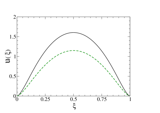
Figure 1: (Color online). Pion parton distribution function. Solid line: full calculation from Eqs. (7) and (8), by using the solution of the BSE, evaluated through the NIR approach and adopting the values of the three input parameters $m=255$ MeV, $\mu=637.5$ MeV and $\Lambda=306$ MeV (see Ref. [13]). Dashed line: LF valence contribution, from the valence component of the Fock expansion of the pion state, Eq. (9) (see Ref. [13]).

Some comments on the results in Fig. 1 are in order: i) the symmetry of the PDFs, with respect to $\xi=0.5$, is entailed by the charge symmetry, that in turn leads to the expression of the uTDM in the Mandelstam approach given by Eq. (8); ii) for $\xi\to 1$, the amplitude of the lowest Fock state generates a contribution that completely saturates $u(\xi)$; iii) while the full PDF is normalized to 1, as it necessarily follows from the standard normalization of the BS amplitude [26, 13], the valence contribution has norm $P_{val}=0.7$; iv) the $30\%$ depletion is due to the presence of the higher Fock-components in the pion state. Let us remind that the two spin configurations of the quark pair contribute to the valence PDF with different probabilities: $P_{\uparrow\downarrow}=0.57$ and $P_{\uparrow\uparrow}=0.13$, so that one remarkably finds a weight of $\sim 25\%$ from purely relativistic effects carried by the aligned component (see Ref. [13] for more details). Finally, at the initial scale, the exponent of $(1-\xi)^{\eta_{0}}$ for $\xi\to 1$ for the full PDF is $\eta_{0}=1.4$.

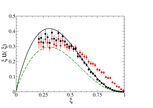
Figure 2: (Color online). The distribution function $\xi~{}u(\xi)$ in a pion. Solid line: full calculation (see Eqs. (7) and (8)), obtained from the BS amplitude solution of the BSE with $m=255$ MeV, $\mu=637.5$ MeV and $\Lambda=306$ MeV, and evolved from the initial scale $Q_{0}=0.360$ GeV to $Q=5.2$ GeV (see text). Dashed line: the evolved LF valence component, Eq. (9). Full dots: experimental data from Ref. [35]. Full squares: reanalyzed data by using the ratio between the fit 3 of Ref. [36], evolved to $5.2$ GeV, and the experimental data [35], at each data point, so that the resummation effects (see text) are accounted for.

An ECLO evolution, as given in Ref. [6], has been applied to the PDFs in Fig. 1 in order to compare our results to the E615 data [35] (measured in Drell-Yan processes), and also taking into account the reanalysis carried out in both Ref. [37], where the scale $4.0$ GeV of the original experimental data was suggested to be moved to $Q=5.2$ GeV, and Ref. [36], where resummation effects on the extraction of the pion PDF were proposed. In particular, Fig. 2 shows the comparison between i) the theoretical calculations, full PDF and valence contribution, evolved to $Q=5.2$ GeV, ii) the data originally delivered by the E615 Collaboration (assigned scale $4.0$ GeV) and iii) the experimental data rescaled, at each $\xi$, by the ratio between the fit 3 in Ref. [36], properly evolved to $5.2$ GeV, and the E615 experimental data. Noteworthy, the calculations in Ref. [36] have illustrated at which extent the PDF extraction from the experimental measurements is affected by the resummation of the large logarithmic contributions in the partonic hard-scattering cross sections. It should be pointed out that the behavior of the evolved $\xi~{}u(\xi)$ for $\xi\to 1$ is given by $(1-\xi)^{\eta_{5}}$ with $\eta_{5}=2.94$ (with $\xi\in[0.9,1]$), to be compared, e.g., to the value $2.20\pm 0.64$ obtained by using recent LQCD calculations [12], where the PDF is reconstructed via Mellin moments, as well as the exponent $2.81\pm 0.08$ reported in Ref. [6]. The low-order Mellin moments for two scales, $Q=2.0$ GeV and $5.2$ GeV, obtained from our pion PDF (after properly evolving through ECLO) and from the most recent LQCD results (with $m_{\pi}=260$ MeV)  [34, 12] are presented in Table 1.

Table 1: Low-order Mellin moments at two scales $Q=2.0$ GeV and $5.2$ GeV. First column: results from our BSE approach, i.e. by using Eqs. (7) and (8) evolved to the scale $Q=2.0$ GeV from an initial scale $Q_{0}=0.360$ GeV (see text). Second column: LQCD calculations at $Q=2.0$ GeV from Ref. [34] for $\langle x\rangle$, and Ref. [12] for $\langle x^{2}\rangle$ and $\langle x^{3}\rangle$, with the errors given by statistical and systematic uncertainties added in quadrature. Third column: our results evolved to $5.2$ GeV. Fourth column: lattice result, evaluated by using the reconstructed PDF, as given in Table XI of Ref. [12].

	BSE2	LQCD2	BSE5	LQCD5
$~{}~{}\langle x\rangle~{}~{}~{}$	0.259	0.261$\pm$0.007	0.221	0.229$\pm$0.008
$\langle x^{2}\rangle$	0.105	0.110$\pm$0.014	0.082	0.087$\pm$0.009
$\langle x^{3}\rangle$	0.052	0.024$\pm$0.018	0.039	0.042$\pm$0.010
$\langle x^{4}\rangle$	0.029		0.021	0.023$\pm$0.009
$\langle x^{5}\rangle$	0.018		0.012	0.014$\pm$0.007
$\langle x^{6}\rangle$	0.012		0.008	0.009$\pm$0.005

Finally, in Fig. 3, the comparison is carried out with some recent theoretical outcomes obtained from different frameworks. The so-called continuum-QCD, based on the Dyson-Schwinger equation and the BSE, is able to yield the PDF, via Mellin moments evaluated in Euclidean space. In particular, we compare with the results presented i) in Ref. [6], where the PDF is obtained from the leading-twist two-particle distribution amplitude (actual calculations are from Ref. [38]), that depends upon only the anti-aligned component of the BS amplitude, and ii) in Ref. [8], where the quark vertex is properly dressed (cfr. the bare vertex $\gamma^{+}$ in Eq. (8)). Moreover, it is shown the PDF directly calculated within the BLFQ in Ref. [11, 39], and the PDF recently evaluated in LQCD by the ETM Collaboration [12], by using the Mellin moments for the reconstruction. Interestingly, the JAM NLO global fit analysis [40] largely overlaps the original E615 data [35]. It is rewarding that our dynamical calculation in Minkowski space falls in the LQCD band and nicely agrees on the tail with the recent calculations from both the DSE approach [6] and the BLFQ one [11, 39].

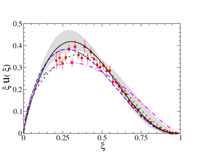
Figure 3: (Color online). The distribution function $\xi~{}u(\xi)$ in a pion, at scale $5.2$ GeV. Solid line: full calculation as in Fig. 2. Dashed line: DSE calculation from Fig. 5 of Ref.  [6]. Dash-dotted line: DSE calculation with dressed quark-photon vertex from Ref. [8]. Dotted line: BLFQ result  [11, 39] . Shaded area: LQCD calculation extracted via Mellin moments from Ref. [12].

Summary. For the first time, the pion PDF has been calculated directly in Minkowski space, within a dynamical framework based on the 4D Bethe-Salpeter equation. We have adopted the Nakanishi integral representation of the BS amplitude, so that the analytic behavior of the BS amplitude can be exposed and manipulated, formally obtaining an equation for the so-called Nakanishi weight functions from the BSE. At this stage of development of our technology, only three parameters enter in the ladder kernel, namely: the masses of quarks and gluon, and the scale of the extended quark-gluon vertex. The initial scale of our calculation is fixed at $Q_{0}=0.360$ GeV (cfr. Ref. [6]). The comparison with data and theoretical calculations are very encouraging and strongly motivates improvements of our approach. In fact, we are currently working on including a consistent treatment of quark and gluon self-energies (see, e.g., Refs. [41, 42]).

Acknowledgments. E. Y. gratefully thanks INFN Sezione di Roma for providing the computer resources to perform all the calculations shown in this work. W. d. P. acknowledges the support from CNPq Grants No. 438562/2018-6 and No. 313030/2021-9, and CAPES Grant No. 88881.309870/2018-01. T. F. acknowledges the support from CNPq (Grant No. 308486/2015-3) and FAPESP (Grants No. 17/05660-0 and No. 2019/07767-1). J. H. A. N. acknowledges the support from FAPESP Grant No. 2014/19094-8. E. Y. acknowledges the support from FAPESP Grant No. 2016/25143 and No. 2018/21758-2. This work is a part of the project Instituto Nacional de Ciência e Tecnologia - Física Nuclear e Aplicações Proc. No. 464898/2014-5.

References

- Aguilar et al. [2019] A. C. Aguilar et al., Pion and Kaon Structure at the Electron-Ion Collider, Eur. Phys. J. A 55, 190 (2019), arXiv:1907.08218 [nucl-ex] .
- Accardi et al. [2016] A. Accardi et al., Electron Ion Collider: The Next QCD Frontier: Understanding the glue that binds us all, Eur. Phys. J. A 52, 268 (2016), arXiv:1212.1701 [nucl-ex] .
- Anderle et al. [2021] D. P. Anderle et al., Electron-ion collider in China, Front. Phys. (Beijing) 16, 64701 (2021), arXiv:2102.09222 [nucl-ex] .
- Salpeter and Bethe [1951] E. E. Salpeter and H. A. Bethe, A Relativistic Equation for Bound-State Problems, Phys. Rev. 84, 1232 (1951).
- Biernat et al. [2014] E. P. Biernat, F. Gross, T. Peña, and A. Stadler, Confinement, quark mass functions, and spontaneous chiral symmetry breaking in Minkowski space, Phys. Rev. D 89, 016005 (2014), arXiv:1310.7545 [hep-ph] .
- Cui et al. [2022] Z. F. Cui, M. Ding, J. M. Morgado, K. Raya, D. Binosi, L. Chang, J. Papavassiliou, C. D. Roberts, J. Rodríguez-Quintero, and S. M. Schmidt, Concerning pion parton distributions, Eur. Phys. J. A 58, 10 (2022), arXiv:2112.09210 [hep-ph] .
- Deur et al. [2016] A. Deur, S. J. Brodsky, and G. F. de Teramond, The QCD Running Coupling, Nucl. Phys. 90, 1 (2016), arXiv:1604.08082 [hep-ph] .
- Bednar et al. [2020] K. D. Bednar, I. C. Cloët, and P. C. Tandy, Distinguishing Quarks and Gluons in Pion and Kaon Parton Distribution Functions, Phys. Rev. Lett. 124, 042002 (2020), arXiv:1811.12310 [nucl-th] .
- Cui et al. [2020] Z.-F. Cui, M. Ding, F. Gao, K. Raya, D. Binosi, L. Chang, C. D. Roberts, J. Rodríguez-Quintero, and S. M. Schmidt, Kaon and pion parton distributions, Eur. Phys. J. C 80, 1064 (2020).
- Lan et al. [2020] J. Lan, C. Mondal, S. Jia, X. Zhao, and J. P. Vary, Pion and kaon parton distribution functions from basis light front quantization and QCD evolution, Phys. Rev. D 101, 034024 (2020), arXiv:1907.01509 [nucl-th] .
- Lan et al. [2022] J. Lan, K. Fu, C. Mondal, X. Zhao, and j. P. Vary (BLFQ), Light mesons with one dynamical gluon on the light front, Phys. Lett. B 825, 136890 (2022), arXiv:2106.04954 [hep-ph] .
- Alexandrou et al. [2021a] C. Alexandrou, S. Bacchio, I. Cloët, M. Constantinou, K. Hadjiyiannakou, G. Koutsou, and C. Lauer (ETM), Pion and kaon from lattice QCD and PDF reconstruction from Mellin moments, Phys. Rev. D 104, 054504 (2021a), arXiv:2104.02247 [hep-lat] .
- de Paula et al. [2021] W. de Paula, E. Ydrefors, J. Alvarenga Nogueira, T. Frederico, and G. Salmè, Observing the Minkowskian dynamics of the pion on the null-plane, Phys. Rev. D 103, 014002 (2021), arXiv:2012.04973 [hep-ph] .
- Ydrefors et al. [2021] E. Ydrefors, W. de Paula, J. H. A. Nogueira, T. Frederico, and G. Salmé, Pion electromagnetic form factor with Minkowskian dynamics, Phys. Lett. B 820, 136494 (2021), arXiv:2106.10018 [hep-ph] .
- Nakanishi [1971] N. Nakanishi, Graph Theory and Feynman Integrals (Gordon and Breach, New York, 1971).
- de Paula et al. [2016] W. de Paula, T. Frederico, G. Salmè, and M. Viviani, Advances in solving the two-fermion homogeneous Bethe-Salpeter equation in Minkowski space, Phys. Rev. D 94, 071901 (2016).
- de Paula et al. [2017] W. de Paula, T. Frederico, G. Salmè, M. Viviani, and R. Pimentel, Fermionic bound states in Minkowski-space: Light-cone singularities and structure, Eur. Phys. Jou. C 77, 764 (2017), arXiv:1707.06946 [hep-ph] .
- Mandelstam [1955] S. Mandelstam, Dynamical variables in the Bethe-Salpeter formalism, Proc. Roy. Soc. Lond. A 233, 248 (1955).
- Alvarenga Nogueira et al. [2018] J. Alvarenga Nogueira, C.-R. Ji, E. Ydrefors, and T. Frederico, Color-suppression of non-planar diagrams in bosonic bound states, Phys. Lett. B 777, 207 (2018), arXiv:1710.04398 [hep-th] .
- Llewellyn-Smith [1969] C. H. Llewellyn-Smith, A relativistic formulation for the quark model for mesons, Annals Phys. 53, 521 (1969).
- Carbonell and Karmanov [2010] J. Carbonell and V. A. Karmanov, Solving Bethe-Salpeter equation for two fermions in Minkowski space, Eur. Phys. J. A 46, 387 (2010), arXiv:1010.4640 [hep-ph] .
- Dudal et al. [2014] D. Dudal, O. Oliveira, and P. J. Silva, Källén-Lehmann spectroscopy for (un)physical degrees of freedom, Phys. Rev. D 89, 014010 (2014), arXiv:1310.4069 [hep-lat] .
- Rojas et al. [2013] E. Rojas, J. P. B. C. de Melo, B. El-Bennich, O. Oliveira, and T. Frederico, On the Quark-Gluon Vertex and Quark-Ghost Kernel: Combining Lattice Simulations with Dyson-Schwinger equations, JHEP 10, 193, arXiv:1306.3022 [hep-ph] .
- Oliveira et al. [2020] O. Oliveira, T. Frederico, and W. de Paula, The soft-gluon limit and the infrared enhancement of the quark-gluon vertex, Eur. Phys. J. C 80, 484 (2020), arXiv:2006.04982 [hep-ph] .
- Zyla et al. [2020] P. A. Zyla et al. (Particle Data Group), Review of Particle Physics, PTEP 2020, 083C01 (2020).
- Lurié et al. [1965] D. Lurié, A. J. Macfarlane, and Y. Takahashi, Normalization of Bethe-Salpeter Wave Functions, Phys. Rev. 140, B1091 (1965).
- Barone et al. [2002] V. Barone, A. Drago, and P. G. Ratcliffe, Transverse polarisation of quarks in hadrons, Phys. Rept. 359, 1 (2002), arXiv:hep-ph/0104283 .
- Fanelli et al. [2016] C. Fanelli, E. Pace, G. Romanelli, G. Salmè, and M. Salmistraro, Pion Generalized Parton Distributions within a fully covariant constituent quark model, Eur. Phys. J. C 76, 253 (2016), arXiv:1603.04598 [hep-ph] .
- Ydrefors et al. [2022] E. Ydrefors, W. de Paula, T. Frederico, and G. Salmé, Pion unpolarized transverse-momentum distribution with Minkowskian dynamics, in preparation (2022).
- Londergan et al. [2010] J. T. Londergan, J. C. Peng, and A. W. Thomas, Charge Symmetry at the Partonic Level, Rev. Mod. Phys. 82, 2009 (2010), arXiv:0907.2352 [hep-ph] .
- Chang and Yan [1973] S.-J. Chang and T.-M. Yan, Quantum field theories in the infinite momentum frame. II. Scattering matrices of scalar and Dirac fields, Phys. Rev. D 7, 1147 (1973).
- Yan [1973] T.-M. Yan, Quantum Field Theories in the Infinite-Momentum Frame. IV. Scattering Matrix of Vector and Dirac Fields and Perturbation Theory, Phys. Rev. D 7, 1780 (1973).
- Brodsky et al. [1998] S. J. Brodsky, H.-C. Pauli, and S. S. Pinsky, Quantum chromodynamics and other field theories on the light cone, Phys. Rept. 301, 299 (1998), arXiv:hep-ph/9705477 [hep-ph] .
- Alexandrou et al. [2021b] C. Alexandrou, S. Bacchio, I. Cloet, M. Constantinou, K. Hadjiyiannakou, G. Koutsou, and C. Lauer (ETM), Mellin moments and for the pion and kaon from lattice QCD, Phys. Rev. D 103, 014508 (2021b), arXiv:2010.03495 [hep-lat] .
- Conway et al. [1989] J. Conway et al., Experimental Study of Muon Pairs Produced by 252-GeV Pions on Tungsten, Phys. Rev. D 39, 92 (1989).
- Aicher et al. [2010] M. Aicher, A. Schäfer, and W. Vogelsang, Soft-gluon resummation and the valence parton distribution function of the pion, Phys. Rev. Lett. 105, 252003 (2010), arXiv:1009.2481 [hep-ph] .
- Wijesooriya et al. [2005] K. Wijesooriya, P. E. Reimer, and R. J. Holt, The pion parton distribution function in the valence region, Phys. Rev. C 72, 065203 (2005), arXiv:nucl-ex/0509012 .
- Chang et al. [2013] L. Chang, I. Cloët, J. Cobos-Martinez, C. Roberts, S. Schmidt, and P. Tandy, Imaging dynamical chiral symmetry breaking: pion wave function on the light front, Phys. Rev. Lett. 110, 132001 (2013), arXiv:1301.0324 [nucl-th] .
- Lan [2022] J. Lan, Meson Structure from Basis Light Front Quantization, Ph.D. thesis, Chinese Academy of Sciences (2022).
- Barry et al. [2018] P. Barry, N. Sato, W. Melnitchouk, and C.-R. Ji, First Monte Carlo Global QCD Analysis of Pion Parton Distributions, Phys. Rev. Lett. 121, 152001 (2018), arXiv:1804.01965 [hep-ph] .
- Jia et al. [2020] S. Jia, P. Maris, D. C. Duarte, T. Frederico, W. de Paula, and E. Ydrefors, Minkowski-space solutions of the Schwinger-Dyson equation for the fermion propagator with the rainbow-ladder truncation, in 18th International Conference on Hadron Spectroscopy and Structure (2020) pp. 560–564, arXiv:1912.00063 [nucl-th] .
- Mezrag and Salmè [2021] C. Mezrag and G. Salmè, Fermion and Photon gap-equations in Minkowski space within the Nakanishi Integral Representation method, Eur. Phys. J. C 81, 34 (2021), arXiv:2006.15947 [hep-ph] .