A Representation-Theoretic Approach to $qq$-Characters

A Representation-Theoretic Approach
to $\bm{qq}$-Characters

Henry LIU

H. Liu

Mathematical Institute, University of Oxford, Andrew Wiles Building,
Radcliffe Observatory Quarter, Woodstock Road, Oxford, OX26GG, UK liu@maths.ox.ac.uk http://people.maths.ox.ac.uk/liu/

Received May 15, 2022, in final form November 17, 2022; Published online November 24, 2022

We raise the question of whether (a slightly generalized notion of) $qq$-characters can be constructed purely representation-theoretically. In the main example of the quantum toroidal $\mathfrak{gl}_{1}$ algebra, geometric engineering of adjoint matter produces an explicit vertex operator $\mathsf{RR}$ which computes certain $qq$-characters, namely Hirzebruch $\chi_{y}$-genera, completely analogously to how the R-matrix $\mathsf{R}$ computes $q$-characters. We give a geometric proof of the independence of preferred direction for the refined vertex in this and more general non-toric settings.

$qq$-characters; geometric engineering; vertex operators; R-matrices; Pandharipande–Thomas theory

17B37; 17B67; 14N35

1 Introduction

From a high vantage point, one could say this paper studies the character theory of representations $V$ of quantum affine (or affinized) algebras $U_{q}(\widehat{\mathfrak{g}})$. In the pioneering work [12], from the R-matrix defining $U_{q}(\widehat{\mathfrak{g}})$, Frenkel and Reshetikhin constructed the $q$-character $\chi_{\mathrm{q}}(V)$, a $q$-analogue of the ordinary character for representations of classical Lie algebras. Later Nakajima [25] provided a geometric construction of $\chi_{\mathrm{q}}(V)$ using his quiver varieties. More recently, in [30], Nekrasov used an analogous geometric construction to produce a one-parameter deformation of $\chi_{\mathrm{q}}(V)$ called the $qq$-character $\chi_{\mathrm{qq}}(V)$. Our main goal will be to bring this collection of ideas full circle back to representation theory, and attempt to fill in the remaining cell of the following table:

$$\begin{array}[]{c|c|c}\text{Construction}&\chi_{\mathrm{q}}&\chi_{\mathrm{qq}}\\ \hline\cr\text{Rep. theory}&\cite[cite]{[\@@bibref{}{Frenkel1999}{}{}]}&??\\ \text{Geometry}&\cite[cite]{[\@@bibref{}{Nakajima2001}{}{}]}&\cite[cite]{[\@@bibref{}{Nekrasov2016}{}{}]}\end{array}$$

To this end, Section 2 reviews the aforementioned material, proposes a generalized notion of $qq$-character, and poses a sequence of questions on how $\chi_{\mathrm{qq}}$ might be described purely in terms of representation theory, namely using only the operators in $U_{q}(\widehat{\mathfrak{g}})$ (as can be done for $q$-characters). Schematically, we ask if there is an operator $\mathsf{RR}_{W,V}$, analogous to the R-matrix $\mathsf{R}_{W,V}$, such that

$$\mathsf{R}_{W,V}\leadsto\chi_{\mathrm{q}}(V),\qquad\mathsf{RR}_{W,V}\leadsto\chi_{\mathrm{qq}}(V)$$ (1.1)

are analogous procedures. We anticipate that such a definition/description of $\chi_{\mathrm{qq}}$ will be useful, among other applications, for studying the enumerative geometry of curves in 3-folds [22].

From a much lower, down-to-earth vantage point, this paper actually mainly studies geometric engineering [15, 20], a procedure by which certain K-theoretic Nekrasov partition functions can be computed using networks of refined topological vertices $C_{\lambda\mu\nu}(q,t)$. This is relevant because

• a specific Nekrasov partition function $Z_{r}$ (for 5d $\mathcal{N}=1^{*}$ supersymmetric $\operatorname{SU}(r)$ Yang–Mills theory) is the Hirzebruch $\chi_{y}$-genus of the moduli of rank-$r$ instantons, which by our definition is a form of $qq$-character for (the $r$-fold tensor product of) the Fock module $\mathsf{F}$ of the quantum toroidal algebra $U_{q,t}\big{(}\widehat{\vphantom{\rule{1.0pt}{5.5pt}}\smash{\widehat{\mathfrak{gl}}}}_{1}\big{)}$;

• refined vertices have a history of descriptions [3, 16] using operators in $U_{q,t}\big{(}\widehat{\vphantom{\rule{1.0pt}{5.5pt}}\smash{\widehat{\mathfrak{gl}}}}_{1}\big{)}$.

Specifically, in Section 3 we build from refined vertices an operator $\mathsf{RR}_{\mathsf{F},\mathsf{F}}$ which produces $Z_{r}$ in much the same way that the R-matrix $\mathsf{R}_{\mathsf{F},\mathsf{F}}$ produces $\chi_{\mathrm{q}}(\mathsf{F}^{\otimes r})$. In this way, we answer a question from Section 2 for the (important!) example of $U_{q,t}\big{(}\widehat{\vphantom{\rule{1.0pt}{5.5pt}}\smash{\widehat{\mathfrak{gl}}}}_{1}\big{)}$. This result can be degenerated to $U_{q}\big{(}\widehat{\mathfrak{sl}}_{2}\big{)}$.

The main challenge in finding an operator $\mathsf{RR}_{W,V}$ is that $\chi_{\mathrm{qq}}(V)$ is morally quadratic in $V$, while $\chi_{\mathrm{q}}(V)$ is linear (see Question 2.6). For $U_{q,t}\big{(}\widehat{\vphantom{\rule{1.0pt}{5.5pt}}\smash{\widehat{\mathfrak{gl}}}}_{1}\big{)}$, the desired quadratic terms naturally occur in (traces of) the so-called refined $4$-point function, see, e.g., [6]. This is our $\mathsf{RR}_{\mathsf{F},\mathsf{F}}$. Compositions of these 4-point functions are similar to but distinct from higher-rank Carlsson–Nekrasov–Okounkov Ext operators [9], which lack nice closed-form formulas despite an excellent representation-theoretic characterization [27, 29]. In contrast, in Section 3.3, using a standard operator formalism, we give an explicit formula for $\mathsf{RR}_{\mathsf{F},\mathsf{F}}$ involving vertex operators with a curious interaction of the horizontal and vertical subalgebras of $U_{q,t}(\widehat{\vphantom{\rule{1.0pt}{5.5pt}}\smash{\widehat{\mathfrak{gl}}}}_{1})$. Similar results hold for other toroidal algebras if adjoint matter can be engineered.

Of significant independent interest is Section 3.4, where we prove the independence of preferred direction, also known as slicing invariance, of the network of refined vertices which computes $Z_{r}$. This is a commonly-assumed property of appropriate networks [5, 17, 24]. Recent work [2] of Arbesfeld contains a geometric proof if the network is the toric skeleton of a smooth toric $3$-fold. We use a degenerating family of abelian varieties to relax the toric constraint, to allow for suitable non-toric gluings of edges. This should cover all networks in current literature for which independence of preferred direction is expected. The strategy in [2], and for us as well, is to identify refined vertices and partition functions as specific limits of equivariant K-theoretic Pandharipande–Thomas (PT) vertices [36] and partition functions. We believe this geometric approach to be cleaner than the recent purely algebraic proof of [13], despite a dependence on the conjectural K-theoretic DT/PT correspondence.

In accordance with the analogy (1.1), in Section 3.6 we consider $\mathsf{RR}^{\operatorname{PT}}$, the lift of $\mathsf{RR}$ to PT theory, and collect some (conjectural) properties of $\mathsf{RR}$ and $\mathsf{RR}^{\operatorname{PT}}$ which we propose are analogues of certain properties of the R-matrix $\mathsf{R}$.

2 $\bm{qq}$-characters

2.1 The geometric definition

2.1.1.

Let $\Gamma$ be a quiver with vertices indexed by a set $I$. Associated to a doubled and framed version of $\Gamma$ is the Nakajima quiver variety

$$X_{\Gamma}(\bm{w})=\bigsqcup_{\bm{v}}X_{\Gamma}(\bm{v},\bm{w}),$$

where $\bm{v}$ and $\bm{w}$ are dimension vectors of the ordinary and framing vertices respectively in the quiver representation. Recall that $X_{\Gamma}$ is a smooth algebraic symplectic variety. Let $\mathsf{T}=\mathsf{A}\times\mathbb{C}_{\hbar}^{\times}\subset\operatorname{Aut}(X_{\Gamma})$ be a (possibly maximal) torus such that $\mathbb{C}_{\hbar}^{\times}$ scales the symplectic form with weight $\hbar$ and $\mathsf{A}$ preserves the symplectic form.

The important work [25], and later [23, 35], showed that the equivariant K-theory group (of coherent algebraic sheaves)

$$V_{\Gamma}(\bm{w})\coloneqq K_{\mathsf{T}}(X_{\Gamma}(\bm{w}))$$ (2.1)

is a highest-weight module for a quantum group $\mathscr{A}_{\Gamma}$ which is essentially a quantum affinized algebra. For example, when $\Gamma$ is of finite ADE type, $\mathscr{A}_{\Gamma}=U_{q}\big{(}\widehat{\mathfrak{g}}_{\Gamma}\big{)}$ is the quantum affine algebra for (a mild central extension of) the classical Lie algebra $\mathfrak{g}_{\Gamma}$. More relevant for us, if $\Gamma$ is the Jordan quiver, with one vertex and one edge loop, then $\mathscr{A}_{\Gamma}=U_{q,t}\big{(}\widehat{\vphantom{\rule{1.0pt}{5.5pt}}\smash{\widehat{\mathfrak{gl}}}}_{1}\big{)}$ is the quantum toroidal $\mathfrak{gl}_{1}$ algebra, which is morally (but not literally) the quantum affinization of $\widehat{\mathfrak{gl}}_{1}$.

The geometric realization (2.1) is useful for studying the representation theory of quantum groups, e.g., if $\Gamma$ of finite ADE type then modules of the form $V_{\Gamma}(\bm{w})$ form a basis in the Grothendieck ring of all finite-dimensional $\mathscr{A}_{\Gamma}$-modules.

2.1.2.

Associated to each module $V_{\Gamma}(\bm{w})$ is the $qq$-character $\chi_{\mathrm{qq}}(V_{\Gamma}(\bm{w}))$, originally introduced in [30] to study the BPS/CFT correspondence.

Definition 2.1.

Let $\operatorname{\mathcal{T}\mkern-1.5mu{\mathit{aut}}}$ denote the tautological bundle of $X_{\Gamma}$, and let $f(-)$ be a function on $K_{\mathsf{T}}(X_{\Gamma})$ such that $f(\mathcal{E}_{1}+\mathcal{E}_{2})=f(\mathcal{E}_{1})f(\mathcal{E}_{2})$. Set

$$\chi_{\mathrm{qq}}^{(f)}(V_{\Gamma}(\bm{w});m,Q)\coloneqq\sum_{\bm{v}}Q^{\bm{v}}\chi_{\mathsf{T}}\big{(}X_{\Gamma}(\bm{v},\bm{w}),\wedge_{-m}^{\bullet}\big{(}\mathcal{T}^{\vee}\big{)}\otimes f(\operatorname{\mathcal{T}\mkern-1.5mu{\mathit{aut}}})\big{)}.$$ (2.2)

Here $m$ and $Q=(Q_{i})_{i\in I}$ are formal variables, with $Q^{\bm{v}}$ being short for $\prod_{i\in I}Q_{i}^{v_{i}}$, and $\wedge_{-m}^{\bullet}(-)\coloneqq\sum_{i}(-m)^{i}\wedge^{i}(-)$ is an alternating sum of exterior powers, $\mathcal{T}$ is the tangent bundle, and

$$\chi_{\mathsf{T}}(X,\mathcal{F})\coloneqq\sum(-1)^{i}H^{i}(X,\mathcal{F})\in K_{\mathsf{T}}(\mathrm{pt})_{\mathrm{loc}}$$

is the $\mathsf{T}$-equivariant Euler characteristic of a coherent sheaf $\mathcal{F}$. (When $X$ is non-compact but the fixed locus $X^{\mathsf{T}}$ is, $\chi_{\mathsf{T}}$ is defined via $\mathsf{T}$-equivariant localization, hence the subscript $\mathrm{loc}$.)

2.1.3.

Note that (2.2) is not the original (combinatorial!) characterization of $\chi_{\mathrm{qq}}$ from [30, Section 6.1], and instead we have used the geometric formula from [30, Sections 8.3 and 8.4]. The geometric formula arises from integration over a certain moduli of crossed instantons, see [31] for an ADHM-style construction. Algebro-geometrically, this moduli space admits a description and virtual cycle in the style of Oh–Thomas [33].

Combinatorially, (the original) $qq$-characters may be constructed by recursive expansion [10] in a similar fashion as for $q$-characters [11]. This is a great approach for explicit computation, especially for $\mathscr{A}_{\Gamma}$-modules which are not geometrically realizable like in (2.1), but it is not the direction we will take in this paper.

2.1.4.

We have allowed for an arbitrary multiplicative function $f$ in (2.2), while the original $qq$-characters use a specific function $f_{\psi}$ (namely the product of all $f_{\psi,i}$ from (2.5)). We feel that $qq$-characters with more general $f$ should be studied on equal footing, especially in light of connections [22, Section 4.2] between $\chi_{\mathrm{qq}}^{(f)}$ and quantities in the enumerative geometry of curves in $3$-folds where $f$ corresponds exactly to a descendent insertion.

An example, which may be of independent interest, is when $f(-)=\mathcal{O}$ is the trivial constant function, which we denote $f=1$. In this case (2.2) is nothing but the (equivariant) Hirzebruch $\chi_{y}$-genus

$$\chi_{\mathrm{qq}}^{(1)}(V_{\Gamma}(\bm{w});m,Q)=\chi_{\mathsf{T},m}(X_{\Gamma}(\bm{w});Q)\coloneqq\sum_{\bm{v}}Q^{\bm{v}}\chi_{\mathsf{T}}\big{(}X_{\Gamma}(\bm{v},\bm{w}),\wedge_{-m}^{\bullet}\big{(}\mathcal{T}^{\vee}\big{)}\big{)},$$

though our variable is called $m$ instead of $y$.

2.2 The question(s)

2.2.1.

We will now pose a sequence of successively more precise questions about the representation-theoretic nature of $qq$-characters. Let $V_{\Gamma}(\bm{w})$ be a geometric representation of $\mathscr{A}_{\Gamma}$ as in Section 2.1.1.

Question 2.2.

Can the quantity $\chi_{\mathrm{qq}}^{(f)}(V_{\Gamma}(\bm{w});m,Q)$ be expressed purely in terms of operators in $\mathscr{A}_{\Gamma}$ acting on $V_{\Gamma}(\bm{w})$?

This question is motivated by the following observation. The specialization $m=1$ for $qq$-characters gives

$$\chi_{\mathrm{qq}}^{(f)}(V_{\Gamma}(\bm{w});1,Q) =\chi_{\mathsf{T}}\left(X_{\Gamma}(\bm{w}),Q^{\cdots}\cdot\wedge_{-1}^{\bullet}\left(\mathcal{T}^{\vee}\right)\otimes f(\operatorname{\mathcal{T}\mkern-1.5mu{\mathit{aut}}})\right)$$ (2.3)

$$=\chi_{\mathsf{T}}\left(X_{\Gamma}(\bm{w})\times X_{\Gamma}(\bm{w}),Q^{\cdots}\cdot\iota_{\Delta}(f(\operatorname{\mathcal{T}\mkern-1.5mu{\mathit{aut}}}))\right),$$ (2.4)

where in (2.3) we abbreviated $\sum_{\bm{v}}Q^{\bm{v}}$ as $Q^{\cdots}$, and in (2.4) $\iota_{\Delta}$ is the inclusion of the diagonal. Hence (2.4) is the trace, in $V_{\Gamma}(\bm{w})$, of the operator of multiplication by $f(\operatorname{\mathcal{T}\mkern-1.5mu{\mathit{aut}}})$. It is known that such operators always live in a commutative subalgebra of $\mathscr{A}_{\Gamma}\subset\operatorname{End}(V_{\Gamma}(\bm{w}))$; see [23, Section 5.4] (written for cohomology/Yangians, but the general principle still applies).

2.2.2.

For a specific choice of $f$, the $m=1$ specialization is exactly a $q$-character.

Example 2.3.

Let $\Gamma$ be of finite ADE type, and let $\big{\{}\psi_{i}^{\pm}(u)\big{\}}_{i\in I}$ be the Drinfeld generators of the loop Cartan in $\mathscr{A}_{\Gamma}=U_{q}(\widehat{\mathfrak{g}}_{\Gamma})$. Let $\operatorname{\mathcal{T}\mkern-1.5mu{\mathit{aut}}}=\bigoplus_{i}\operatorname{\mathcal{T}\mkern-1.5mu{\mathit{aut}}}_{i}$ be the decomposition across vertices of $\Gamma$, and consider

$$f_{\psi,i}(\operatorname{\mathcal{T}\mkern-1.5mu{\mathit{aut}}})\coloneqq\widehat{S}^{\bullet}\big{(}\big{(}1-\hbar^{-1}\big{)}\otimes\operatorname{\mathcal{T}\mkern-1.5mu{\mathit{aut}}}_{i}\big{)},$$ (2.5)

where $\widehat{S}^{\bullet}(V)\coloneqq\operatorname{Sym}^{\bullet}(V)\otimes(\det V)^{1/2}$ is a “symmetrized” version of the symmetric algebra. Then

$$\psi_{i}^{\pm}(u)=f_{\psi,i}(u\otimes\operatorname{\mathcal{T}\mkern-1.5mu{\mathit{aut}}}),$$ (2.6)

as operators expanded in series around $u^{\pm 1}\to 0$, see, e.g., [25, Theorem 9.4.1]. Therefore $\chi_{\mathrm{qq}}^{(f_{\psi,i})}(V_{\Gamma}(\bm{w});1,Q)$ equals

$$\chi_{q}^{(i)}(V_{\Gamma}(\bm{w});Q)\coloneqq\operatorname{tr}_{V_{\Gamma}(\bm{w})}Q^{\cdots}\psi_{i}^{\pm}(u),$$ (2.7)

also known as the ($i$-th) $q$-character of $V_{\Gamma}(\bm{w})$. Up to some syntactic repackaging, (2.7) is essentially the $q$-character originally introduced in [12] for quantum affine algebras. This explains the nomenclature “$qq$-character”.

2.2.3.

Whenever the canonical bundle $\mathcal{K}_{X}$ admits a square root, there is a natural pairing on $K_{\mathsf{T}}(X)$ given by

$$\langle\mathcal{F}_{1},\mathcal{F}_{2}\rangle_{X}\coloneqq\sum_{i}(-1)^{i}\operatorname{Ext}^{i}_{\mathsf{T}}\big{(}\mathcal{F}_{1},\mathcal{F}_{2}\otimes\mathcal{K}_{X}^{1/2}\big{)},$$ (2.8)

and $\langle\mathcal{F}_{1},\mathcal{F}_{2}\rangle_{X}=(-1)^{\dim X}\langle\mathcal{F}_{2},\mathcal{F}_{1}\rangle_{X}^{\vee}$ if Serre duality applies. Since our $X$ will always be smooth and symplectic, (2.8) becomes a Hermitian form. We therefore use bra-ket notation for elements of $K_{\mathsf{T}}(X)$, along with the shorthand

$$\langle v|A|w\rangle^{\prime}\coloneqq\frac{\langle v|A|w\rangle}{\langle v|w\rangle}.$$

2.2.4.

For our purposes, it is useful to repackage (2.7) as follows. Let $\bm{\delta}_{i}=(0,\ldots,0,1,0,\ldots,0)$ be the dimension vector with $1$ in the $i$-th position only, and consider the highest-weight modules $V_{i}\coloneqq V_{\Gamma}(\bm{\delta}_{i})$. Let $\ket{\varnothing}$ denote the highest weight vector (up to scalars).

Proposition 2.4.

Let $\Gamma$ be of finite ADE type. Let $V$ be a finite-dimensional $\mathscr{A}_{\Gamma}$-module and $\mathsf{R}_{V_{i},V}\in\operatorname{End}(V_{i}\otimes V)$ be the R-matrix. Then

$$\psi_{i}^{\pm}(u)=\langle\varnothing|\mathsf{R}_{V_{i},V}|\varnothing\rangle_{1}^{\prime}\in\operatorname{End}(V),$$ (2.9)

where $\langle-\rangle_{1}$ means to take the matrix element in the first tensor factor $V_{i}$.

In fact, in general the entire Hopf algebra $\mathscr{A}_{\Gamma}$, not just its elements $\psi_{i}^{\pm}(u)$, is constructed from the data of R-matrices $\{\mathsf{R}_{V,V^{\prime}}\}$ where $V$, $V^{\prime}$ range over the modules (2.1) ([37], [35, Section 3] or [23, Section 5] for the cohomological case). When $\Gamma$ has loops, in general $\psi_{i}^{\pm}(u)$ is a product of the matrix elements in the r.h.s. of (2.9).

Proof sketch..

Recall $\mathsf{R}=\operatorname{Stab}_{-}^{-1}\circ\operatorname{Stab}_{+}$ where $\operatorname{Stab}_{\pm}$ are upper-/lower-triangular stable envelopes. So only the diagonal terms, normalized exactly to give (2.6), contribute to $\langle\varnothing|\mathsf{R}|\varnothing\rangle$; see the factorization of $\mathsf{R}$ in [35, Section 2.3] or the cohomological argument in [23, Section 4.7]. ∎

Therefore

$$\chi_{\mathrm{q}}^{(i)}(V;Q)=\operatorname{tr}_{V}Q^{\cdots}\langle\varnothing|\mathsf{R}_{V_{i},V}|\varnothing\rangle_{1}^{\prime}.$$ (2.10)

2.2.5.

In complete analogy with (2.10), a natural refinement of Question 2.2 is the following.

Question 2.5.

Does there exist a highest-weight module $W$ and an operator $\mathsf{RR}_{W,V}(m)$ such that, for appropriate $f$,

$$\chi_{\mathrm{qq}}^{(f)}(V;m,Q)=\operatorname{tr}_{V}Q^{\cdots}\frac{\langle\varnothing|\mathsf{RR}_{W,V}(m)|\varnothing\rangle_{1}^{\prime}}{\langle\varnothing\otimes\varnothing|\mathsf{RR}_{W,V}(m)|\varnothing\otimes\varnothing\rangle^{\prime}},$$ (2.11)

with $\mathsf{RR}_{W,V}(1)=\mathsf{R}_{W,V}$?

With our normalization conventions, $\langle\varnothing\otimes\varnothing|\mathsf{R}_{W,V}|\varnothing\otimes\varnothing\rangle^{\prime}=1$ and therefore this factor was not present in (2.10). For brevity, let

$$\langle\varnothing|\mathsf{RR}|\varnothing\rangle_{1}^{\prime\prime}$$

denote the normalized operator in the r.h.s. of (2.11), so $\chi_{\mathrm{qq}}^{(f)}=\operatorname{tr}Q^{\cdots}\langle\varnothing|\mathsf{RR}|\varnothing\rangle_{1}^{\prime\prime}$.

2.2.6.

We take a very specific and somewhat naive approach to answering Question 2.5 for the modules $V=V_{\Gamma}(\bm{w})$. Let $X=X_{\Gamma}(\bm{w})$, and let $\{\ket{\mathcal{O}_{p}}\}_{p\in X^{\mathsf{T}}}$ be the basis of structure sheaves of fixed points. The operator of multiplication by $\operatorname{\mathcal{T}\mkern-1.5mu{\mathit{aut}}}$ acts diagonally in this basis.

Question 2.6.

Does there exist a highest-weight module $W$ and an operator $\mathsf{RR}_{W,V}(m)$ such that

$$\frac{\wedge_{-m}^{\bullet}(\mathcal{T}_{p}^{\vee})}{\wedge_{-1}^{\bullet}(\mathcal{T}_{p}^{\vee})}=\frac{\left\langle\varnothing\otimes\mathcal{O}_{p}|\mathsf{RR}_{W,V}(m)|\varnothing\otimes\mathcal{O}_{p}\right\rangle^{\prime}}{\left\langle\varnothing\otimes\varnothing|\mathsf{RR}_{W,V}(m)|\varnothing\otimes\varnothing\right\rangle^{\prime}}$$

for every $p\in X^{\mathsf{T}}$?

Such an operator would essentially answer Question 2.5 since, by $\mathsf{T}$-equivariant localization,

$$\chi_{\mathrm{qq}}^{(f)}(V;m,Q)=\operatorname{tr}_{V}Q^{\cdots}f(\operatorname{\mathcal{T}\mkern-1.5mu{\mathit{aut}}})\left\langle\varnothing|\mathsf{RR}_{W,V}(m)|\varnothing\right\rangle_{1}^{\prime\prime}.$$ (2.12)

2.2.7.

In Section 3, we answer the following variant of Question 2.6 in the affirmative for the Jordan quiver $\Gamma$, for which the Nakajima quiver variety $X_{\Gamma}(r)=\mathcal{M}_{r}$ is the moduli of rank-$r$ instantons.

Question 2.7.

Does there exist a highest-weight module $W$ and an operator $\mathsf{RR}_{W,V}(m)$ such that

$$\frac{\wedge_{-m}^{\bullet}(\mathcal{T}_{p}^{\vee})}{\wedge_{-1}^{\bullet}(\mathcal{T}_{p}^{\vee})}=\frac{\left\langle\varnothing\otimes\mathcal{F}_{p}|\mathsf{RR}_{W,V}(m)|\varnothing\otimes\mathcal{F}_{p}\right\rangle^{\prime}}{\left\langle\varnothing\otimes\varnothing|\mathsf{RR}_{W,V}(m)|\varnothing\otimes\varnothing\right\rangle^{\prime}}$$

for every $p\in X^{\mathsf{T}}$, for some basis $\{\ket{\mathcal{F}_{p}}\}_{p\in X^{\mathsf{T}}}$ with nice properties?

One reason to look beyond the basis $\{\ket{\mathcal{O}_{p}}\}$ of fixed points is that fixed points do not behave nicely with respect to tensor product; see Section 3.1.4 for details in the case of $\mathcal{M}_{r}$. For example, any operator $\mathsf{RR}_{W,V}$ satisfying the original Question 2.6 has little hope of satisfying the fusion property of the original R-matrices $\mathsf{R}_{W,V}$ (see Section 3.6.2), but our operator $\mathsf{RR}_{W,V}$ will satisfy Question 2.7 for a basis $\{\ket{\mathcal{O}^{\otimes}_{p}}\}$ preserving this fusion property.

2.2.8.

The discrepancy between Questions 2.6 and 2.7 is exactly the obstruction to incorporating a non-trivial insertion $f$. Namely, we answer Question 2.7 in a basis $\{\ket{\mathcal{O}_{p}^{\otimes}}\}$ where $\operatorname{\mathcal{T}\mkern-1.5mu{\mathit{aut}}}$ does not act diagonally (see Section 3.1.5), and therefore the resulting $\mathsf{RR}_{W,V}(m)$ no longer answers Questions 2.5 or 2.6; only the specific $f=1$ case

$$\chi_{\mathrm{qq}}^{(1)}(V;m,Q)=\operatorname{tr}_{V}Q^{\cdots}\left\langle\varnothing|\mathsf{RR}_{W,V}(m)|\varnothing\right\rangle_{1}^{\prime\prime}$$

of (2.12) continues to hold. To incorporate a general $f$, one could try to rewrite $\mathsf{RR}(m)$ in the true fixed-point basis $\{\ket{\mathcal{O}_{p}}\}$. Put differently, if $\mathsf{S}$ is the change of basis from $\{\ket{\mathcal{O}_{p}}\}$ to $\{\ket{\mathcal{O}_{p}^{\otimes}}\}$, then $\mathsf{S}^{-1}\cdot\mathsf{RR}\cdot\mathsf{S}$ satisfies Question 2.6 if the operator $\mathsf{RR}$ satisfies Question 2.7. However, it is unclear whether there is a representation-theoretic interpretation or formula for $\mathsf{S}$.

2.2.9.

To be clear, the conditions imposed by Questions 2.6 and  2.7 are on the spectrum of the operator $\mathsf{RR}$, while the condition of Question 2.5 is merely on the trace of $\mathsf{RR}$. One therefore expects the former to be far more stringent than the latter. Indeed, we see this explicitly as a consequence of the results in Section 3, where we find many different operators $\mathsf{RR}$ such that

$$\chi_{\mathsf{T},m}(\mathcal{M}_{r};Q)=\operatorname{tr}Q^{\cdots}\langle\varnothing|\mathsf{RR}|\varnothing\rangle_{1}^{\prime\prime}$$

is the Hirzebruch $\chi_{y}$-genus of $\mathcal{M}_{r}$, but only one such $\mathsf{RR}$ has the “correct” diagonal elements.

3 Geometric engineering

3.1 The setup

3.1.1.

Let $\Gamma$ be the Jordan quiver, with one vertex and one edge loop. The Nakajima quiver variety $X_{\Gamma}(r)$ is the moduli

$$\mathcal{M}_{r}\coloneqq\mathcal{M}_{r}(\mathbb{C}^{2})\coloneqq\big{\{}E\in\mathsf{Coh}(\mathbb{P}^{2})\text{ torsion-free}\colon E\big{|}_{\mathbb{P}^{1}_{\infty}}\cong\mathcal{O}_{\mathbb{P}^{1}_{\infty}}^{\oplus r}\big{\}}$$

of rank-$r$ instantons on $\mathbb{C}^{2}$. It admits natural actions induced by $\operatorname{GL}_{2}$ acting on $\mathbb{C}^{2}$, and by $\operatorname{GL}_{r}$ acting on the framing $\mathcal{O}_{\mathbb{P}^{1}_{\infty}}^{\oplus r}$. Let

$$\mathsf{T}\coloneqq\mathsf{T}_{\text{framing}}\times\mathsf{T}_{\mathbb{C}^{2}}\coloneqq(\mathbb{C}^{\times})^{r}\times(\mathbb{C}^{\times})^{2}\ni(a_{1},\ldots,a_{r},q,t)$$

be the maximal torus of this $\operatorname{GL}_{r}\times\operatorname{GL}_{2}$, with coordinates written as above. The $r=1$ case is the Hilbert scheme $\mathcal{M}_{1}=\operatorname{Hilb}$ of points on $\mathbb{C}^{2}$.

3.1.2.

Let $\mathbbm{k}\coloneqq K_{\mathsf{T}}(\mathrm{pt})_{\mathrm{loc}}=\mathbb{Z}\big{[}a_{1}^{\pm},\ldots,a_{r}^{\pm},q^{\pm},t^{\pm}\big{]}_{\mathrm{loc}}$ where $\mathrm{loc}$ means to adjoin $(1-w)^{-1}$ for all non-zero monomials $w\in K_{\mathsf{T}}(\mathrm{pt})$. All our modules and computations are implicitly over this base ring. Set

$$\mathsf{F}\coloneqq K_{\mathsf{T}}(\operatorname{Hilb}).$$

The quantum group associated to $\Gamma$ is the quantum toroidal $\mathfrak{gl}_{1}$ algebra $\mathscr{A}_{\Gamma}=U_{q,t}\big{(}\widehat{\vphantom{\rule{1.0pt}{5.5pt}}\smash{\widehat{\mathfrak{gl}}}}_{1}\big{)}$, and $\mathsf{F}$ is its standard Fock module. See Section 3.3.1 for some more details. By general principles [23], stable envelopes provide an isomorphism of $\mathscr{A}_{\Gamma}$-modules

$$\operatorname{Stab}\colon\ \mathsf{F}^{\otimes r}\otimes\mathbbm{k}\xrightarrow{\sim}K_{\mathsf{T}}(\mathcal{M}_{r})\otimes\mathbbm{k}.$$ (3.1)

Stable envelopes can be viewed as “corrected” versions of (the pushforward along) the inclusion

$$\iota\colon\ (\mathcal{M}_{r})^{\mathsf{T}_{\text{framing}}}=\operatorname{Hilb}^{\times r}\hookrightarrow\mathcal{M}_{r}$$

of the $\mathsf{T}_{\text{framing}}$-fixed locus, which itself only induces an isomorphism of $\mathbbm{k}$-modules.

3.1.3.

The $\mathsf{T}_{\mathbb{C}^{2}}$-fixed points of $\operatorname{Hilb}$, and therefore basis elements of $\mathsf{F}$, are labeled by partitions $\lambda$. The $\mathsf{T}$-fixed points of $\mathcal{M}_{r}$ are therefore $r$-tuples $\bm{\lambda}=\big{(}\lambda^{(1)},\ldots,\lambda^{(r)}\big{)}$ of partitions. So here we fix some notation for partitions.

We will use the letters $\lambda$, $\mu$, $\nu$ to denote partitions. Occasionally it is useful to view a partition $\lambda=(\lambda_{1},\lambda_{2},\ldots)$ in terms of its Young diagram. Let $(i,j)=(i(\square),j(\square))$ be the position of a square $\square\in\lambda$ in the Young diagram. If $\lambda^{t}$ is the conjugate partition, set

$$a(\square)\coloneqq\lambda_{i(\square)}-j(\square),\qquad\ell(\square)\coloneqq\big{(}\lambda^{t}\big{)}_{j(\square)}-i(\square).$$

Let $|\lambda|\coloneqq\sum_{i}\lambda_{i}$ denote the size of $\lambda$.

3.1.4.

We identify $\mathsf{F}$ with the algebra of symmetric functions. From (2.8), there is a standard inner product $\langle-,-\rangle$ on $\mathsf{F}$. We will use two bases in $\mathsf{F}$:

• the basis of Schur polynomials $s_{\lambda}$, which are orthonormal;

• the basis of fixed points $\mathcal{O}_{\lambda}$, which are orthogonal with norm

  $$\langle\mathcal{O}_{\lambda},\mathcal{O}_{\lambda}\rangle=(qt)^{\frac{|\lambda|}{2}}\prod_{\square\in\lambda}\big{(}1-q^{-\ell(\square)-1}t^{a(\square)}\big{)}\big{(}1-q^{\ell(\square)}t^{-a(\square)-1}\big{)}.$$

  This can also be taken as the definition of $\langle-,-\rangle$ if desired. Let $\widetilde{\mathcal{O}}_{\lambda}$ be the unit vector normalization of $\mathcal{O}_{\lambda}$, so they form an orthonormal basis.

The elements $\mathcal{O}_{\lambda}\in\mathsf{F}$ are Haiman’s normalization of Macdonald polynomials, e.g., denoted $\widetilde{H}_{\lambda}$ in [14].

3.1.5.

We identify $\mathsf{F}^{\otimes r}$ with $K_{\mathsf{T}}(\mathcal{M}_{r})$ using (3.1). The tensor product $\mathsf{F}^{\otimes r}$ inherits the inner product from $\mathsf{F}$; note that this is not the inner product on $K_{\mathsf{T}}(\mathcal{M}_{r})$ from (2.8). We consider two bases in $\mathsf{F}^{\otimes r}$:

• the basis of generalized Schur polynomials $s_{\bm{\lambda}}\coloneqq\otimes_{i=1}^{r}s_{\lambda^{(i)}}$, which are orthonormal;

• the basis of fixed points $\mathcal{O}_{\bm{\lambda}}$, also known as generalized Macdonald polynomials (see, e.g., [6], cf. [39]), which are not orthogonal.

The latter is not the same as

$$\mathcal{O}^{\otimes}_{\bm{\lambda}}\coloneqq\otimes_{i=1}^{r}\mathcal{O}_{\lambda^{(i)}}\in\mathsf{F}^{\otimes r},$$

which do form an orthonormal basis. This is because although $\mathcal{O}_{\bm{\lambda}}=\iota_{*}\boxtimes_{i=1}^{r}\mathcal{O}_{\lambda^{(i)}}$ as sheaves on $\mathcal{M}_{r}$, the identification (3.1) is not $\iota_{*}$. A crucial distinguishing property is that, in general,

$$\mathcal{O}_{(\lambda^{(1)},\lambda^{(2)})}\neq\mathcal{O}_{\lambda^{(1)}}\otimes\mathcal{O}_{\lambda^{(2)}}.$$

3.2 The $\bm{\chi_{y}}$-genus

3.2.1.

Our primary goal is to study the $\chi_{y}$-genus $\chi_{\mathsf{T},m}(\mathcal{M}_{r};Q)$, and various representation-theoretic description of it in terms of operators in the algebra $U_{q,t}\big{(}\widehat{\vphantom{\rule{1.0pt}{5.5pt}}\smash{\widehat{\mathfrak{gl}}}}_{1}\big{)}$. The strategy is to compute the $\chi_{y}$-genus via a form of geometric engineering, which equates it to the refined partition functions of certain special toric $3$-folds. One consequence, among others, of our computations is an affirmative answer (Theorem 3.3) to Question 2.7.

3.2.2.

Refined partition functions in the toric setting are (sums of) products of contributions $C_{\lambda\mu\nu}(q,t)$, called refined vertices, from each toric chart. One labels each edge of the toric $1$-skeleton with a partition and performs certain combinatorial sums over them; see [17] for details. For example,

$$\vbox{\hbox{\includegraphics[scale={1.1}]{images/refined-vertex.pdf}}}=C_{\lambda\mu\nu}(q,t),\qquad\vbox{\hbox{\includegraphics[scale={1.1}]{images/refined-vertex-glued-2.pdf}}}=\sum_{\lambda}Q^{|\lambda|}C_{\lambda\mu_{1}\nu_{1}}(q,t)C_{\lambda^{t}\mu_{2}\nu_{2}}(t,q).$$

Here a marked half-edge labels the “preferred direction” $\nu$ of the vertex $C_{\lambda\mu\nu}$, which is necessary because it is not symmetric in $\lambda$, $\mu$, $\nu$. (This asymmetry is evident in the explicit formula (3.9) later.) An unlabeled half-edge is set to $\varnothing$, and any other edge not explicitly labeled by a partition is summed over. Each edge may be labeled with a so-called Kähler variable, e.g., $Q$, indicating a term $Q^{|\cdot|}$ recording the size of the partition on the edge. The result is a function of $q$, $t$, and various Kähler variables.

Remark 3.1.

For the experts, all our edges will have normal bundles $\mathcal{O}(-1)^{\oplus 2}$, i.e., everything is locally a conifold, so we neglect framing factors when gluing refined vertices.

3.2.3.

Different choices of toric diagram engineer different quantities on $\mathcal{M}_{r}$, or more generally $\mathcal{M}_{r_{1}}\times\cdots\times\mathcal{M}_{r_{k}}$, and a general recipe is given in [20]. However, it is important that the diagram does not need to be the $1$-skeleton of an actual toric $3$-fold for geometric engineering to work. In particular, the $\chi_{y}$-genus involves gluing edges in the following non-toric way.

Proposition 3.2.

With the substitution $t\mapsto t^{-1}$,

$$\chi_{\mathsf{T},\kappa}(\mathcal{M}_{r};Q)=\vbox{\hbox{\includegraphics[scale={1.1}]{images/adjoint-matter-diagram.pdf}}}\bigg{/}\vbox{\hbox{\includegraphics[scale={1.1}]{images/adjoint-matter-perturbative-diagram.pdf}}}$$ (3.2)

where the half-edges with the same variable $Q_{i}$ are glued together, i.e., there is an additional overall sum $\sum_{\lambda_{1},\ldots,\lambda_{r}}Q_{1}^{|\lambda_{1}|}\cdots Q_{r}^{|\lambda_{r}|}$, and there are identifications

$$Q_{1}=\cdots=Q_{r}=Q,\qquad A_{1}=\cdots=A_{r}=\kappa,\qquad A_{k}B_{k}=a_{k+1}/a_{k}.$$ (3.3)

Proof.

By explicit calculation using the formalism in [15] (or otherwise). ∎

In physics language, Proposition 3.2 gives the “toric” diagram for engineering adjoint $U(r)$ matter. The denominator is referred to as the perturbative term, and has an explicit closed form formula unimportant to us.

3.2.4.

Let $Z_{r}\big{(}q,t^{-1};Q,A,\bm{B}\big{)}$ be the quantity encoded by the numerator of (3.2); since all the $Q_{i}$ are specialized to be equal, we retain only a single variable denoted $Q$, and similarly for the $A_{i}$ and $A$. For clarity, $Z_{r}$ is written out explicitly in (3.10).

Let $\bm{\lambda}=\big{(}\lambda^{(1)},\lambda^{(2)},\ldots,\lambda^{(r)}\big{)}$ be the partitions labeling the horizontal legs of (3.2), so that we can write the individual contributions of the diagram with fixed horizontal legs as

$$Z_{r}(q,t;Q,A,\bm{B})\eqqcolon\sum_{\bm{\lambda}}Q^{|\bm{\lambda}|}Z_{r}(q,t;A,\bm{B})_{\bm{\lambda}}.$$

For example, the denominator of (3.2) is $Z_{r}(\cdots)_{\bm{\varnothing}}$.

Theorem 3.3.

There is an operator $\mathsf{RR}\in\operatorname{End}(\mathsf{F}\otimes\mathsf{F})[[Q,A]]$, with explicit formula given by (3.8), such that

$$\big{(}{-}\sqrt{qt}\big{)}^{|\bm{\lambda}|}Z_{r}\big{(}q,t^{-1};A,A\bm{B}\big{)}_{\bm{\lambda}}$$

$$\qquad{}=\big{\langle}\varnothing\otimes\mathcal{O}^{\otimes}_{\bm{\lambda}}\big{|}\mathsf{RR}^{(10)}B_{1}^{|\cdot|}\mathsf{RR}^{(20)}B_{2}^{|\cdot|}\cdots B_{r-1}^{|\cdot|}\mathsf{RR}^{(r0)}\big{|}\varnothing\otimes\mathcal{O}^{\otimes}_{\bm{\lambda}}\big{\rangle},$$ (3.4)

where $\mathsf{RR}^{(ij)}$ means to act on the $i$-th and $j$-th tensor factors and the $B_{i}^{|\cdot|}$ act in the $0$-th tensor factor.

3.2.5.

In fact, the proof of Proposition 3.2 proceeds by identifying

$$\frac{\wedge^{\bullet}_{-\kappa}\big{(}\mathcal{T}_{\bm{\lambda}}^{\vee}\big{)}}{\wedge^{\bullet}_{-1}\big{(}\mathcal{T}_{\bm{\lambda}}^{\vee}\big{)}}=\frac{Z_{r}(\cdots)_{\bm{\lambda}}}{Z_{r}(\cdots)_{\bm{\varnothing}}}$$

up to the identifications (3.3). Hence Theorem 3.3 resolves Question 2.7 in the affirmative for $\mathcal{M}_{r}$. Note that the operator

$$\big{\langle}\varnothing\big{|}\mathsf{RR}^{(10)}B_{1}^{|\cdot|}\mathsf{RR}^{(20)}B_{2}^{|\cdot|}\cdots B_{r-1}^{|\cdot|}\mathsf{RR}^{(r0)}\big{|}\varnothing\big{\rangle}\in\operatorname{End}\big{(}\mathsf{F}^{\otimes r}\big{)}$$

is closely related to but is not exactly the higher-rank Carlsson–Nekrasov–Okounkov Ext operator [9], for which no explicit vertex operator formula is known. The diagonal matrix elements match but off-diagonal ones differ by some explicit factors. The higher-rank Ext operator is a well-studied object in part due to its role in the AGT correspondence, see, e.g., [28], and it would be interesting to relate known characterizations of it to our explicit operator.

3.2.6.

Taking the trace of (3.4) gives

$$Z_{r}\big{(}q,t^{-1};-Q\sqrt{qt},A,A\bm{B}\big{)}=\operatorname{tr}_{\mathsf{F}^{\otimes r}}Q^{|\cdot|}\big{\langle}\varnothing\big{|}\mathsf{RR}^{(10)}B_{1}^{|\cdot|}\mathsf{RR}^{(20)}B_{2}^{|\cdot|}\cdots B_{r-1}^{|\cdot|}\mathsf{RR}^{(r0)}\big{|}\varnothing\big{\rangle}_{0},$$ (3.5)

where $\left\langle-,-\right\rangle_{0}$ means the matrix element is taken in the $0$-th tensor factor. We will construct different operators $\mathsf{RR}^{H}$ and $\mathsf{RR}^{V}$ which both satisfy (3.5) up to mild changes of variables (nb. the discussion of Section 2.2.9). The key idea (Theorem 3.13) is that the diagrams in (3.2) remain the same under any choice of preferred direction for the refined vertices. In particular, $\mathsf{RR}^{H}$ (resp. $\mathsf{RR}^{V}$) arises from horizontal (resp. vertical) preferred direction. The effects, not always trivial, of changing the preferred direction can be investigated quite generally for toric diagrams possibly with some pairs of parallel half-edges glued together (in a non-toric way), and so Section 3.4 is of independent interest.

3.3 An explicit operator formula

3.3.1.

The algebra $U_{q,t}\big{(}\widehat{\vphantom{\rule{1.0pt}{5.5pt}}\smash{\widehat{\mathfrak{gl}}}}_{1}\big{)}$ is complicated; see [38] for various presentations. For us, it suffices to know that it contains two special subalgebras:

• the “horizontal” Heisenberg subalgebra, with generators $\{\alpha_{n}\}_{n\in\mathbb{Z}}$ which in terms of power-sum polynomials $p_{k}\in\mathsf{F}$ act as

  $$\alpha_{n}=n\frac{\partial}{\partial p_{n}},\qquad\alpha_{-n}=p_{n},\qquad\forall n>0;$$

• the “vertical” commutative subalgebra, with generators $\{H_{n}\}_{n\in\mathbb{Z}}$ which act on fixed points as $H_{n}\cdot\mathcal{O}_{\lambda}=h_{n}(\lambda;q,t)\mathcal{O}_{\lambda}$ with eigenvalue

  $$h_{n}(\lambda;q,t)\coloneqq\operatorname{sign}(n)\left(-\chi_{\lambda}(q^{n},t^{n})+\frac{1}{(1-q^{n})(1-t^{n})}\right)$$ (3.6)

  where $\chi_{\lambda}(q,t)\coloneqq\sum_{\square\in\lambda}q^{i(\square)}t^{j(\square)}$. One recognizes this as the weight of the tautological bundle of $\operatorname{Hilb}$ at the fixed point $\lambda$.

Experts will notice that the action of $\alpha_{-n}$ for $n>0$ is scaled by a factor $-\big{(}q^{n/2}-q^{-n/2}\big{)}\big{(}t^{n/2}-t^{-n/2}\big{)}$ from the usual horizontal generators.

3.3.2.

Let

$$\Gamma_{+}(z)\coloneqq\exp\left(\sum_{n>0}(qt)^{\frac{n}{2}}\big{(}t^{\frac{n}{2}}-t^{-\frac{n}{2}}\big{)}(H_{n}\otimes\alpha_{n})\frac{z^{n}}{n}\right),$$

$$\Gamma_{-}(z)\coloneqq\exp\left(-\sum_{n>0}(qt)^{-\frac{n}{2}}\big{(}q^{\frac{n}{2}}-q^{-\frac{n}{2}}\big{)}(H_{-n}\otimes\alpha_{-n})\frac{z^{-n}}{n}\right).$$ (3.7)

Furthermore let $\mathsf{D}$ be the diagonal operator whose entries are $\big{\langle}\widetilde{\mathcal{O}}_{\lambda}|\mathsf{D}|\widetilde{\mathcal{O}}_{\lambda}\big{\rangle}\coloneqq\langle\mathcal{O}_{\lambda}|\mathcal{O}_{\lambda}\rangle^{-1}$.

Theorem 3.4.

$$\mathsf{RR}=\mathsf{RR}^{H}\coloneqq\mathsf{D}^{(1)}\Gamma_{-}\big{(}\sqrt{qt}\big{)}^{-1}\Gamma_{+}(1)^{-1}\Gamma_{-}(-A)\Gamma_{+}\big{(}{-}1/A\sqrt{qt}\big{)},$$ (3.8)

where a superscript $(-)^{(1)}$ means to act on the first tensor factor.

3.3.3.

Explicit formulas like (3.8), particularly the “vertex operators” $\Gamma_{\pm}(z)$, have some precursors in the literature under the name of Awata–Feigin–Shiraishi or Ding–Iohara–Miki intertwiners [3]. In some sense, the main novelty in our computation is the introduction of the auxiliary factor of $\mathsf{F}$ where the operators $H_{\pm n}$ (in (3.7)) from the vertical subalgebra of $U_{q,t}\big{(}\widehat{\vphantom{\rule{1.0pt}{5.5pt}}\smash{\widehat{\mathfrak{gl}}}}_{1}\big{)}$ act. The operators $\Gamma_{\pm}(z)$ involve a curious interaction of the vertical and horizontal subalgebras, in contrast to objects living only in one slope subalgebra $U_{q,t}\big{(}\widehat{\mathfrak{gl}}_{1}\big{)}\subset U_{q,t}\big{(}\widehat{\vphantom{\rule{1.0pt}{5.5pt}}\smash{\widehat{\mathfrak{gl}}}}_{1}\big{)}$, e.g., the vertex operators in the R-matrix [26]. Alternatively, one can view them as single-slope objects evaluated on $\mathsf{F}^{V}\otimes\mathsf{F}$ instead of $\mathsf{F}\otimes\mathsf{F}$, where $\Phi\colon U_{q,t}\big{(}\widehat{\vphantom{\rule{1.0pt}{5.5pt}}\smash{\widehat{\mathfrak{gl}}}}_{1}\big{)}\to\operatorname{End}\big{(}\mathsf{F}^{V}\big{)}$ is the “vertical” Fock representation [29].

3.3.4.

We now proceed with the proof of Theorem 3.4. The refined vertex with preferred direction $\nu$ is

$$C_{\lambda\mu\nu}(q,t)\coloneqq\left(\frac{t}{q}\right)^{\frac{\|\mu\|^{2}+\|\nu\|^{2}}{2}}\!\!q^{\frac{\kappa(\mu)}{2}}P_{\nu^{t}}(q,t)\sum_{\eta}\left(\frac{t}{q}\right)^{\frac{|\eta|+|\lambda|-|\mu|}{2}}\!\!s_{\lambda^{t}/\eta}\big{(}q^{-\rho}t^{-\nu}\big{)}s_{\mu/\eta}\big{(}t^{-\rho}q^{-\nu^{t}}\big{)},\!\!\!$$ (3.9)

where the $s_{\lambda/\mu}(\bm{x})$ are skew Schur functions, $q^{-\rho}t^{-\nu}$ means $\big{(}q^{1/2}t^{-\nu_{1}},q^{3/2}t^{-\nu_{2}},q^{5/2}t^{-\nu_{3}},\ldots\big{)}$, $\|\mu\|^{2}\coloneqq\sum_{i}\mu_{i}^{2}$ and $\kappa(\mu)\coloneqq\|\mu\|^{2}-\|\mu^{t}\|^{2}$, and

$$P_{\nu^{t}}(q,t)\coloneqq q^{\frac{\|\nu\|^{2}}{2}}\prod_{\square\in\nu}\frac{1}{1-q^{\ell(\square)+1}t^{a(\square)}}.$$

Setting $\nu^{(0)}\coloneqq\nu^{(r)}\coloneqq\varnothing$, the desired quantity is

$$Z_{r}\big{(}q,t^{-1};Q,A,\bm{B}\big{)}=\sum_{\nu^{(1)},\ldots,\nu^{(r-1)}}\prod_{i=1}^{r}B_{i}^{|\nu^{(i)}|}Z_{\nu^{(i-1)},\nu^{(i)t}}^{H}\big{(}q,t^{-1};Q,A\big{)},$$ (3.10)

where $Z_{\nu,\nu^{\prime}}^{H}$ is the so-called four-point diagram

$$\vbox{\hbox{\includegraphics[scale={1.1}]{images/four-point-diagram-horizontal.pdf}}}\eqqcolon{} Z_{\nu^{(1)},\nu^{(2)t}}^{H}\big{(}q,t^{-1};Q,A\big{)}$$

$$={} \sum_{\lambda,\mu}A^{|\mu|}Q^{|\lambda|}C_{\mu\nu^{(1)}\lambda}\big{(}q,t^{-1}\big{)}C_{\mu^{t}\nu^{(2)t}\lambda^{t}}\big{(}t^{-1},q\big{)}$$

$$={} \sum_{\lambda,\mu,\eta_{1},\eta_{2}}Q^{|\lambda|}A^{|\nu^{(2)}|}(qt)^{\frac{\|\lambda^{t}\|^{2}-\|\lambda\|^{2}}{2}}P_{\lambda}\big{(}t^{-1},q\big{)}P_{\lambda^{t}}\big{(}q,t^{-1}\big{)}$$

$$\qquad\quad\ {}\times s_{\mu^{t}/\eta_{1}}\big{(}q^{-\rho}t^{\lambda}\big{)}s_{\nu^{(1)}/\eta_{1}}\big{(}(qt)^{\frac{1}{2}}q^{-\lambda^{t}}t^{\rho}\big{)}$$

$$\qquad\quad\ {}\times s_{\mu/\eta_{2}}\big{(}Aq^{-\lambda^{t}}t^{\rho}\big{)}s_{\nu^{(2)t}/\eta_{2}}\big{(}A^{-1}(qt)^{-\frac{1}{2}}q^{-\rho}t^{\lambda}\big{)}.$$ (3.11)

The superscript $H$ reminds us that the horizontal direction is preferred. In the second equality above, we used the homogeneity $z^{|\lambda|-|\mu|}s_{\lambda/\mu}(\bm{x})=s_{\lambda/\mu}(z\bm{x})$ to absorb some factors of $A$ and $\sqrt{qt}$.

3.3.5.

The following key tool converts a skew Schur function into a matrix element of an operator on $\mathsf{F}$.

Lemma 3.5 ([18, Chapter 14]).

$$s_{\lambda/\mu}(\bm{x})=\left\langle s_{\mu}\bigg{|}\exp\left(\sum_{n>0}p_{n}(\bm{x})\frac{\alpha_{n}}{n}\right)\bigg{|}s_{\lambda}\right\rangle.$$ (3.12)

We will need two transformations that can be performed on (3.12), that leave the l.h.s. unchanged but modify the r.h.s.:

• transposing the operator, to get $s_{\lambda/\mu}(\bm{x})=\left\langle s_{\lambda}|\exp(\cdots\alpha_{-n}\cdots)|s_{\mu}\right\rangle$;

• applying the $\omega$-involution on $\mathsf{F}$, to get $s_{\lambda/\mu}(\bm{x})=\left\langle s_{\mu^{t}}|\exp(-\cdots p_{n}(-\bm{x})\cdots)|s_{\lambda^{t}}\right\rangle$.

3.3.6.

For arguments $\bm{x}=q^{-\rho}t^{\nu}$ or similar, Lemma 3.5 for $s_{\lambda/\mu}(\bm{x})$ is better interpreted as a matrix element of an operator on $\mathsf{F}\otimes\mathsf{F}$.

Lemma 3.6.

$$s_{\lambda/\mu}(q^{-\rho}t^{\nu})=\left\langle\widetilde{\mathcal{O}}_{\nu}\otimes s_{\mu}\bigg{|}\exp\left(-\sum_{n>0}\big{(}qt)^{n/2}(t^{n/2}-t^{-n/2}\big{)}\frac{H_{n}\otimes\alpha_{n}}{n}\right)\bigg{|}\widetilde{\mathcal{O}}_{\nu}\otimes s_{\lambda}\right\rangle,$$

$$s_{\lambda/\mu}(q^{-\nu^{t}}t^{\rho})=\left\langle\widetilde{\mathcal{O}}_{\nu}\otimes s_{\mu}\bigg{|}\exp\left(\sum_{n>0}(qt)^{-n/2}\big{(}q^{n/2}-q^{-n/2}\big{)}\frac{H_{-n}\otimes\alpha_{n}}{n}\right)\bigg{|}\widetilde{\mathcal{O}}_{\nu}\otimes s_{\lambda}\right\rangle.$$

Proof.

For $n>0$,

$$p_{n}\big{(}q^{-\rho}t^{\nu}\big{)}=q^{n/2}\sum_{k>0}q^{n(k-1)}t^{n\nu_{k}}=-(qt)^{n/2}\big{(}t^{n/2}-t^{-n/2}\big{)}h_{n}(\nu;q,t),$$

where $h_{n}(\nu;q,t)$ is the eigenvalue of $H_{n}$ on the fixed point $\mathcal{O}_{\nu}$, as in (3.6). Similarly,

$$p_{n}\big{(}q^{-\nu^{t}}t^{\rho}\big{)}=(qt)^{-n/2}\big{(}q^{n/2}-q^{-n/2}\big{)}h_{-n}(\nu^{t};t,q),$$

but quite clearly $h_{n}(\nu^{t};t,q)=h_{n}(\nu;q,t)$. ∎

3.3.7.

It is clear that the terms in the last two lines of (3.11) eventually become the vertex operators, via Lemma 3.6, so the terms in the first line must be absorbed somewhere. Compute that

$$(qt)^{\frac{\|\lambda^{t}\|^{2}-\|\lambda\|^{2}}{2}}P_{\lambda^{t}}\big{(}q,t^{-1}\big{)}P_{\lambda}\big{(}t^{-1},q\big{)} =q^{\frac{\|\lambda^{t}\|^{2}}{2}}t^{-\frac{\|\lambda\|^{2}}{2}}\prod_{\square\in\lambda}\frac{1}{1-q^{\ell(\square)+1}t^{-a(\square)}}\frac{1}{1-q^{\ell(\square)}t^{-a(\square)-1}}$$

$$=(-1)^{|\lambda|}(qt)^{\frac{|\lambda|}{2}}\frac{1}{\langle\mathcal{O}_{\lambda}|\mathcal{O}_{\lambda}\rangle}$$ (3.13)

using that $\sum_{\square\in\lambda}\ell(\square)=\big{(}\|\lambda^{t}\|^{2}-|\lambda|\big{)}/2$ and similarly for $a(\square)$. The resulting $\big{(}{-}\sqrt{qt}\big{)}^{|\lambda|}$ term is absorbed into the Kähler variable $Q$. Finally, the term $\langle\mathcal{O}_{\lambda}|\mathcal{O}_{\lambda}\rangle^{-1}$ comes from $\mathsf{D}$.

3.4 Dependence on preferred direction

3.4.1.

The way in which diagrams such as the ones in (3.2) depend on the choice of preferred direction has been raised [17] and studied, e.g., [5], since the introduction of the refined vertex. A good way to study this dependence is to relate the refined vertex $C_{\lambda\mu\nu}(q,t)$ to the more symmetric K-theoretic Pandharipande–Thomas (PT) vertex $V_{\lambda\mu\nu}(x,y,z;\mathfrak{q})$.

For a review of (equivariant) K-theoretic DT and PT theory, [34] should suffice.

Definition 3.7.

Let $\mathsf{T}\coloneqq(\mathbb{C}^{\times})^{3}$ with coordinates $(x,y,z)$. Given a function $f(x,y,z)$ on $\mathsf{T}$ and a cocharacter $\sigma(u)=\big{(}u^{a},u^{b},u^{c}\big{)}\in\mathsf{T}$, let

$$\lim_{\sigma}f\coloneqq\lim_{u\to 0}f(\sigma(u)).$$

If $a+b+c=0$, i.e., $\sigma$ preserves $\kappa\coloneqq xyz$, and there is some permutation of $a$, $b$, $c$ so that $a\gg b>0$, then $\sigma$ is called an index limit.

Theorem 3.8 ([32, Theorem 2]).

Assume the DT/PT conjecture [32, formula (16)] for equivariant K-theoretic vertices. Then

$$(\text{\rm prefactor})\cdot C_{\lambda\mu\nu}\big{(}{-}\mathfrak{q}\kappa^{\frac{1}{2}},-\mathfrak{q}\kappa^{-\frac{1}{2}}\big{)}=\lim_{\sigma_{V}}V_{\lambda\mu\nu}(x,y,z;\mathfrak{q})$$

for the index limit $\sigma_{V}(u)\coloneqq\big{(}u^{N},u^{-N-1},u\big{)}$ with $N\gg 0$.

The PT vertex $V_{\lambda\mu\nu}$ is fully symmetric in its three legs, upon permuting the variables $x$, $y$, $z$ accordingly, so different permutations of components of the cocharacter $\sigma_{V}$ produce refined vertices with different preferred direction.

In general, therefore, refined partition functions $Z$ are index limits of analogous PT partition functions

$$Z^{\operatorname{PT}}(x,y,z;\mathfrak{q},Q,A,\bm{B})\in\mathbb{Q}\big{(}x^{\frac{1}{2}},y^{\frac{1}{2}},z^{\frac{1}{2}}\big{)}((\mathfrak{q}))[[Q,A,\bm{B}]],$$ (3.14)

built from the PT vertex $V_{\lambda\mu\nu}$ (and PT edge contributions) in the same way that $Z$ is built from the refined vertex $C_{\lambda\mu\nu}$. Changing preferred direction in $Z$ corresponds to changing the index limit $\sigma$ for $Z^{\operatorname{PT}}$, which we can study geometrically. This sort of approach first appeared in [2] for toric geometries, and we now review (a mild, non-toric generalization of) the arguments there in order to prove our Theorem 3.13.

3.4.2.

The new ingredient is the following geometric construction of $Z_{r}^{\operatorname{PT}}$, which is no longer associated directly with an actual toric $3$-fold. We continue to assume the DT/PT conjecture [32, formula (16)] throughout this subsection.

Definition 3.9.

Let $\widetilde{X}$ be the (infinite type) smooth toric $3$-fold given by the periodic toric polytope of Figure 1, where all edges are locally conifolds $\mathcal{O}(-1)^{\oplus 2}$. Let $\mathsf{T}=(\mathbb{C}^{\times})^{3}$ be its standard torus. Let $\Lambda_{r}\cong\mathbb{Z}^{2}$ be the translation action on the polytope with generators as shown in the figure, acting on coordinates as

$$(x,y,z)\mapsto\big{(}\kappa x,\kappa^{-1}y,z\big{)},\qquad(x,y,z)\mapsto\big{(}x,\kappa^{-r}y,\kappa^{r}z\big{)}$$ (3.15)

for $\kappa\coloneqq xyz$.

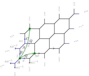
Figure 1: The periodic toric diagram defining $\widetilde{X}$, with generators of the translation action $\Lambda_{2}$ in green and the fundamental region in blue. Some coordinates and some Kähler variables are indicated.

Theorem 3.10 ([1]).

There exists a well-defined quotient

$$X_{r}\coloneqq\widetilde{X}/\Lambda_{r}\to\operatorname{Spec}\mathbb{C}[[\kappa]]$$

such that the map to $\operatorname{Spec}\mathbb{C}[[\kappa]]$ is proper and flat.

This $X_{r}$ has already appeared explicitly in [19], but it is an instance of a far more general construction of (degenerating) families of abelian varieties due to Alexeev [1], where the initial combinatorial data is an arbitrary periodic toric polytope. In general, the generic fiber is an abelian variety while the special fiber is some union of toric varieties. The prototypical, rank-$1$ example of Alexeev’s construction is the Tate elliptic curve $k^{\times}/q^{\mathbb{Z}}\to\operatorname{Spec}k[[q]]$.

3.4.3.

The torus $\mathsf{T}$ acting on $\widetilde{X}$ can be identified with $\mathbb{C}_{\kappa}^{\times}\times(\mathbb{C}^{\times})^{2}$ where $\mathbb{C}_{\kappa}^{\times}$ scales the coordinate $\kappa$ on the base. On the quotient $X_{r}$, localization with respect to $\mathbb{C}_{\kappa}^{\times}$ restricts our attention to the compact special fiber, which is a union of toric varieties for the remaining $(\mathbb{C}^{\times})^{2}$. Hence the $\mathsf{T}$-equivariant PT theory of $X_{r}$ is well-defined, and the vertex formalism is still applicable and yields exactly the desired non-toric gluings.

Definition 3.11.

Let $\operatorname{PT}(X_{r})$ be the moduli scheme of PT pairs on $X_{r}$ and $\widehat{\mathcal{O}}^{\mathrm{vir}}\in K_{\mathsf{T}}(\operatorname{PT}(X_{r}))$ be its symmetrized virtual structure sheaf; see, e.g., [34, Section 3.2] for details. (The symmetrization necessitates passing to a double cover of $\mathsf{T}$, hence the square roots in (3.14).) Consider the $\mathsf{T}$-equivariant K-theoretic pushforward

$$Z_{r}^{\operatorname{PT}}(x,y,z;\mathfrak{q};Q,A,\bm{B})\coloneqq\chi_{\mathsf{T}}\big{(}\operatorname{PT}(X_{r}),\widehat{\mathcal{O}}^{\mathrm{vir}}\cdot\mathfrak{q}^{|\cdot|}Q^{\cdots}A^{\cdots}\bm{B}^{\cdots}C^{\cdots}\big{)}\big{|}_{C=0},$$ (3.16)

where $\mathfrak{q}$ is the boxcounting parameter and the Kähler variables $Q,A,\bm{B},C$ record curve classes as indicated in Figure 1, in exactly the same way as for the refined partition function $Z_{r}$. To match with $Z_{r}$, we set $C=0$ to disallow non-trivial curves (i.e., partitions) along those edges.

Remark 3.12.

The identifications (3.3) of the Kähler variables $Q$ and $\bm{A}$ come from the relations of their corresponding curve classes in $H_{2}\big{(}\widetilde{X},\mathbb{Z}\big{)}$, and therefore in $H_{2}(X_{r},\mathbb{Z})$ as well, by examining the hexagons in Figure 1. In contrast, it is not necessary to specialize the $B_{i}$ in any way.

3.4.4.

The proof the following theorem will occupy the remainder of this subsection.

Theorem 3.13.

With the specializations (3.3), we have

$$Z_{r}=\lim_{\sigma}Z_{r}^{\operatorname{PT}}$$

which furthermore is independent of the choice of index limit $\sigma$. In particular, (3.2) can be computed under any choice of preferred direction.

Note that the construction of $Z^{\operatorname{PT}}$ and its independence of $\sigma$ is much more generally applicable to any toric diagram with appropriate non-toric gluings, not just our diagram for $Z_{r}$. In particular there is no need to set $C=0$ in (3.16), in which case there are obvious so-called “triality” symmetries in the diagram of Figure 1, see, e.g., [7].

3.4.5.

The PT vertex $V_{\lambda\mu\nu}(x,y,z;\mathfrak{q})$ (and PT edges) enjoys a number of nice properties, chief among which is that it is a sum of so-called “balanced” rational functions of the form

$$\prod_{i}\frac{(\kappa w_{i})^{1/2}-(\kappa w_{i})^{-1/2}}{w_{i}^{1/2}-w_{i}^{-1/2}},\qquad\kappa\coloneqq xyz,$$ (3.17)

for monomials $w_{i}=w_{i}(x,y,z)$. (This follows immediately from the construction of $\widehat{\mathcal{O}}^{\mathrm{vir}}$.) We refer to the $w_{i}$ as poles of the rational function.

Lemma 3.14.

Let $\sigma$ and $\tau$ be cocharacters such that $\kappa(\sigma(u))$ and $\kappa(\tau(u))$ are independent of $u$. Let $f$ be a balanced rational function, as in (3.17). Then

$$\lim_{\sigma}f=\lim_{\tau}f$$

if $\lim_{\sigma}w_{i}=\lim_{\tau}w_{i}$ for every pole $w_{i}$ of $f$.

Being built from PT vertices (and edges), $Z_{r}^{\operatorname{PT}}(x,y,z)$ is also a sum of balanced rational functions. Hence the behavior of $\lim_{\sigma}Z_{r}^{\operatorname{PT}}$ is controlled by the poles of $Z_{r}^{\operatorname{PT}}$, and it suffices to locate these poles.

Note that individual components, e.g., the PT vertices $V_{\lambda\mu\nu}^{\operatorname{PT}}$ comprising the sum $Z_{r}^{\operatorname{PT}}$, may have more poles than $Z_{r}^{\operatorname{PT}}$ does; there will generally be some pole cancellation which we will now explain.

3.4.6.

Pole-cancellation is controlled by the following geometric observation.

Proposition 3.15 ([2, Proposition 3.2]).

Let $\mathcal{M}$ be a space with action by a torus $\mathsf{T}$. Let $\mathcal{F}$ be a $($virtual$)$ sheaf on $\mathcal{M}$ and assume that $($virtual$)$ $\mathsf{T}$-equivariant localization is applicable to $\chi_{\mathsf{T}}(\mathcal{M},\mathcal{F})$. Then its poles occur only at weights $w\in\operatorname{Hom}(\mathsf{T},\mathbb{C}^{\times})$ such that the fixed locus $\mathcal{M}^{\ker w}$ is non-compact.

Proof.

If $\mathcal{M}^{\ker w}$ were compact, then equivariant localization with respect to the maximal torus $\mathsf{T}_{w}\subset\ker w\subset\mathsf{T}$ produces poles only at $\mathsf{T}$-weights occuring in the (virtual) normal bundle $\mathcal{N}_{\mathcal{M}/\mathcal{M}^{\mathsf{T}w}}$, none of which vanish on $\mathsf{T}_{w}$ (by definition of the normal bundle). ∎

In the case of PT theory of a $3$-fold $X$, the only way for $\operatorname{PT}(X)^{\ker w}$ to be non-compact is if $\ker w$ leaves some non-compact direction in $X$ invariant – e.g., if $X$ is toric and $w$ is an integer power of the weight of some half-edge in the toric diagram – and there are complete curves in $X$ which can escape to infinity along that direction. This is a reflection of the fact that there is a Hilbert–Chow map

$$\pi\colon\ \operatorname{PT}(X)\to\operatorname{Chow}(X),$$

which is proper on each component of the Chow variety of $1$-dimensional cycles on $X$, and so non-compact directions in $\operatorname{PT}(X)$ must arise from $\operatorname{Chow}(X)$. We have arrived at the conclusion of [2]: weights of such non-compact directions in $X$ form walls in the cocharacter lattice, and $\lim_{\sigma}Z^{\operatorname{PT}}$ can only change when $\sigma$ crosses a wall.

3.4.7.

We now move beyond the results of [2], where this pole-cancellation principle is applied only to toric $3$-folds. Our $X_{r}$ is not toric, but the same argument as in Section 3.4.6 applies. The only non-compact direction in $X_{r}$ is along the base $\operatorname{Spec}\mathbb{C}[[\kappa]]$, and so all poles of $Z_{r}^{\operatorname{PT}}$ occur only at integer powers of $\kappa$. By Lemma 3.14, such poles do not affect index limits, which by definition leave $\kappa$ constant. Hence $\lim_{\sigma}Z_{r}^{\operatorname{PT}}$ is independent of index limit $\sigma$, as desired.

3.4.8.

Finally, it remains to verify that $Z_{r}=\lim_{\sigma}Z_{r}^{\operatorname{PT}}$. The only non-trivial step is with computing the index limit of PT edge contributions in $X_{r}$, for the half-edges which are glued together in a non-toric way. This is done via the following trivial observation.

Lemma 3.16.

In the setting of Proposition 3.14, modifying any weight $w_{i}$ by multiples of $\kappa$ does not affect $\lim_{\sigma}f$.

In particular, this applies to coordinate changes $(x,y,z)\mapsto\big{(}\kappa^{a}x,\kappa^{b}y,\kappa^{c}z\big{)}$ with $a+b+c=0$, and the action of $\Lambda_{r}$ on $\widetilde{X}$ is generated by substitutions of this form. In other words, $Z_{r}^{\operatorname{PT}}$ may change under the substitutions of (3.15), but $\lim_{\sigma}Z_{r}^{\operatorname{PT}}$ does not. Hence, for each pair of half-edges glued in a non-toric way, e.g., one in coordinates $(x,y,z)$ and another in coordinates $(\kappa^{a}x,\kappa^{-a}y,z)$, we are free to pick either of the two coordinate charts to write the edge term.

Example 3.17.

In our setting, all edges are local conifolds, i.e., having normal bundle $\mathcal{O}(-1)^{\oplus 2}$. Let $E_{\lambda}$ be the PT edge contribution for a curve of class $\lambda$ on such an edge. Then in rank $r=1$,

$$\lim_{\sigma}\left(\vbox{\hbox{\includegraphics[scale={1.1}]{images/four-point-1.pdf}}}\right)\eqqcolon\lim_{\sigma}\big{(}Z_{1}^{\operatorname{PT}}(x,y,z;\mathfrak{q},Q,A,C=0)\big{)}$$

$$\qquad=\lim_{\sigma}\bigg{(}\sum_{\lambda,\mu}Q^{|\lambda|}A^{|\mu|}V_{\lambda\mu\varnothing}(x,y,z;\mathfrak{q})V_{\lambda^{t}\mu^{t}\varnothing}\big{(}yz,y^{-1},xy;\mathfrak{q}\big{)}E_{\lambda}(x,y,z;\mathfrak{q})E_{\mu}(y,z,x;\mathfrak{q})\bigg{)},$$

where, equally well, $E_{\lambda}(x,y,z;\mathfrak{q})$ could be have been replaced by $E_{\lambda^{t}}\big{(}yz,y^{-1},xy;\mathfrak{q}\big{)}$.

In general, by Theorem 3.8, the PT vertex $V_{\lambda\mu\nu}$ becomes the refined vertex $C_{\lambda\mu\nu}$ (with appropriate preferred direction) up to some prefactors which are combinatorial quantities in $\lambda$, $\mu$, and $\nu$. One can check by explicit computation that

$$\lim_{\sigma}E_{\lambda}=q^{\frac{\|\lambda\|^{2}}{2}}t^{\frac{\|\lambda^{t}\|^{2}}{2}}$$

exactly cancels these prefactors, e.g., the part of the prefactor from the vertex which depends on $\lambda$ is $q^{-\|\lambda\|^{2}/2}(q/t)^{|\lambda|}$, and the vertex on the other end of the edge contributes $t^{-\|\lambda^{t}\|^{2}/2}(t/q)^{|\lambda^{t}|}$. See [2, Section 4.3] for details. We conclude that prefactors and edges don’t matter, and ${\lim_{\sigma}Z_{r}^{\operatorname{PT}}=Z_{r}}$ is just a combination of refined vertices, as claimed.

3.5 Another explicit operator formula

3.5.1.

From Theorem 3.13, the desired partition function $Z_{r}\big{(}q,t^{-1};Q,A,\bm{B}\big{)}$ can also be computed using four-point diagrams with vertical preferred direction:

$$\vbox{\hbox{\includegraphics[scale={1.1}]{images/four-point-diagram-vertical.pdf}}}\eqqcolon{} Z_{\nu^{(1)},\nu^{(2)t}}^{V}\big{(}q,t^{-1};Q,A\big{)}$$

$$={} \sum_{\lambda,\mu,\eta_{1},\eta_{2}}(QA)^{|\lambda|}\left(qt\right)^{\frac{\|\nu^{(2)t}\|^{2}-\|\nu^{(1)}\|^{2}}{2}}P_{\nu^{(1)t}}\big{(}q,t^{-1}\big{)}P_{\nu^{(2)}}\big{(}q,t^{-1}\big{)}$$

$$\qquad\quad\ {}\times s_{\lambda^{t}/\eta_{1}}\big{(}A^{-1}q^{-\rho}t^{\nu^{(1)}}\big{)}s_{\mu/\eta_{1}}\big{(}(qt)^{\frac{1}{2}}Aq^{-\nu^{(1)t}}t^{\rho}\big{)}$$

$$\qquad\quad\ {}\times s_{\lambda/\eta_{2}}\big{(}q^{-\nu^{(2)t}}t^{\rho}\big{)}s_{\mu^{t}/\eta_{2}}\big{(}(qt)^{-\frac{1}{2}}q^{-\rho}t^{\nu^{(2)}}\big{)},$$

cf. (3.11). This is completely distinct from the horizontal version $Z_{\nu^{(1)},\nu^{(2)t}}^{H}$. Note also that the Kähler variable $A$ is distributed slightly differently this time.

3.5.2.

We introduce a new “mixing” operator

$$\mathsf{M}\coloneqq\sum_{\lambda,\mu}\ket{\widetilde{\mathcal{O}}_{\lambda}}\bra{\widetilde{\mathcal{O}}_{\mu}}.$$

Theorem 3.18.

$$Z_{r}\big{(}q,t^{-1};QA,A,-\bm{B}\sqrt{qt}\big{)}=\operatorname{tr}_{\mathsf{F}^{\otimes r}}Q^{|\cdot|}\big{\langle}\varnothing\big{|}\big{(}\mathsf{RR}^{V}\big{)}^{(01)}\!B_{1}^{|\cdot|}\big{(}\mathsf{RR}^{V}\big{)}^{(02)}\!B_{2}^{|\cdot|}\cdots B_{r-1}^{|\cdot|}\big{(}\mathsf{RR}^{V}\big{)}^{(0r)}\!\big{|}\varnothing\big{\rangle},$$

where the $B_{i}^{|\cdot|}$ and matrix element are taken in the $0$-th tensor factor, and

$$\mathsf{RR}^{V}=\mathsf{D}^{(1)}\Gamma_{+}(1)^{-1}\Gamma_{-}\big{(}1/\sqrt{qt}\big{)}^{-1}\cdot\mathsf{M}^{(1)}\cdot\Gamma_{+}\big{(}{-}A\sqrt{qt}\big{)}\Gamma_{-}(-1/A),$$ (3.18)

where a superscript $(-)^{(1)}$ means to act on the first tensor factor.

3.5.3.

The proof of Theorem 3.18 is completely analogous to that of Theorem 3.4 for $\mathsf{RR}^{H}$, and so we only provide some comments for the purpose of comparison.

• The mixing operator $\mathsf{M}$ is necessary because for any given four-point function, two of the skew Schur functions involve $\nu^{(i)}$ while the other two involve $\nu^{(i+1)}$.

• The computation (3.13) now takes place not within a single four-point function, but across two different ones. Explicitly, $\lambda$ in (3.13) is replaced by $\nu\coloneqq\nu^{(i)}$ for a fixed $i$. The resulting $\big{(}{-}\sqrt{qt}\big{)}^{|\nu|}$ term now must be absorbed by the Kähler variables $\bm{B}$.

3.5.4.

We make a few comments on the form of (3.18). For general rank $r$, Theorem 3.13 guarantees that the operators

$$\big{\langle}\varnothing\big{|}\big{(}\mathsf{RR}^{V}\big{)}^{(01)}\cdots\big{(}\mathsf{RR}^{V}\big{)}^{(0r)}\big{|}\varnothing\big{\rangle},\;\big{\langle}\varnothing\big{|}\big{(}\mathsf{RR}^{H}\big{)}^{(10)}\cdots\big{(}\mathsf{RR}^{H}\big{)}^{(r0)}|\varnothing\big{\rangle}\in\operatorname{End}\big{(}\mathsf{F}^{\otimes r}\big{)}$$

have the same trace, despite being manifestly different operators (already evident from the lowest-order off-diagonal term). In the case $r=1$, the operator $\mathsf{M}$ does nothing in $\big{\langle}\varnothing|\mathsf{RR}^{V}|\varnothing\big{\rangle}\in\operatorname{End}(\mathsf{F})$, and one can check that the traces are equal explicitly. This rank-$1$ calculation already appeared in [16, Section 5] in limited generality.

3.6 Properties of $\bm{\mathsf{RR}}$

3.6.1.

We collect here some properties of R-matrices – fusion (Section 3.6.2), unitarity (Section 3.6.3), and the Yang–Baxter equation (Section 3.6.4) – and discuss their analogues for the operator $\mathsf{RR}$. In fact, it is productive to discuss more generally the fully-equivariant four-point function in K-theoretic PT theory, so let

$$\mathsf{RR}^{\operatorname{PT}}(A;x,y,z)\coloneqq\big{(}\big{(}\mathsf{RR}^{\operatorname{PT}}\big{)}^{\mu^{\prime}\nu^{\prime}}_{\mu\nu}\big{)}\coloneqq\left(\vbox{\hbox{\includegraphics[scale={1.1}]{images/four-point-PT.pdf}}}\right)\in\operatorname{End}(\mathsf{F}\otimes\mathsf{F})((A))$$

denote the PT partition function associated to the four-point diagram shown. Explicitly, in the notation of Example 3.17,

$$\big{(}\mathsf{RR}^{\operatorname{PT}}\big{)}^{\mu^{\prime}\nu^{\prime}}_{\mu\nu}\coloneqq\sum_{\lambda}A^{|\lambda|}V_{\mu\lambda\nu}(x,y,z;\mathfrak{q})V_{\mu^{\prime}\lambda^{t}\nu^{\prime}}\big{(}yz,y^{-1},xy;\mathfrak{q}\big{)}E_{\lambda}(y,z,x;\mathfrak{q}).$$

3.6.2.

Recall that if $\mathsf{R}_{W,V_{1}}\in\operatorname{End}(W\otimes V_{1})$ and $\mathsf{R}_{W,V_{2}}\in\operatorname{End}(W\otimes V_{2})$ are R-matrices, then

$$\mathsf{R}_{W,V_{1}\otimes V_{2}}=\mathsf{R}_{W,V_{1}}^{(12)}\mathsf{R}_{W,V_{2}}^{(13)}\in\operatorname{End}(W\otimes V_{1}\otimes V_{2}).$$

In this way, $q$-characters of tensor products arise from R-matrices of each tensor factor. Completely analogously, the factorization of (3.2) into four-point diagrams indicates that we should define

$$\mathsf{RR}^{\operatorname{PT}}_{\mathsf{F},\mathsf{F}\otimes\mathsf{F}}\coloneqq\big{(}\mathsf{RR}^{\operatorname{PT}}_{\mathsf{F},\mathsf{F}}\big{)}^{(12)}B^{|\cdot|}\big{(}\mathsf{RR}^{\operatorname{PT}}_{\mathsf{F},\mathsf{F}}\big{)}^{(13)},$$

and $qq$-characters of tensor products therefore also arise from $\mathsf{RR}$ of each tensor factor. Note that the Kähler variable $B$ becomes some combination of evaluation parameters or equivariant variables under the identification (3.3).

3.6.3.

Recall that if $\mathsf{R}(u)\in\operatorname{End}(V\otimes V)$ is a trigonometric R-matrix with spectral parameter $u$, then it is important to study whether

$$\mathsf{R}^{(21)}\big{(}u^{-1}\big{)}=\mathsf{R}(u),$$

called unitarity. We propose that the following is the analogue for $\mathsf{RR}^{\operatorname{PT}}$.

Conjecture 3.19 (flop invariance).

Let

$$\widetilde{\mathsf{RR}}^{\operatorname{PT}}(A;x,y,z)\coloneqq\frac{\mathsf{RR}^{\operatorname{PT}}(A;x,y,z)}{\mathsf{RR}^{\operatorname{PT}}(A;x,y,z)^{\varnothing\varnothing}_{\varnothing\varnothing}}$$

be the normalization, as in (3.2). Then

$$\widetilde{\mathsf{RR}}^{\operatorname{PT}}\big{(}A^{-1};x,xy,z/x\big{)}^{\mu^{\prime}\nu}_{\mu\nu^{\prime}}=\widetilde{\mathsf{RR}}^{\operatorname{PT}}(A;x,y,z)^{\mu^{\prime}\nu^{\prime}}_{\mu\nu}.$$

The change of variables $(x,y,z)\mapsto(x,xy,z/x)$ is to ensure that each of the four half-edges $\mu$, $\mu^{\prime}$, $\nu$, $\nu^{\prime}$ retains the same weight. (Only the weight of the internal edge changes.)

This conjecture is known, by the explicit computation in [21], when either $\mu=\mu^{\prime}=\varnothing$ or $\nu=\nu^{\prime}=\varnothing$, i.e., only one set of half-edges is non-trivial. In general it is a question about the behavior of DT (or PT) invariants under flops, and such general questions have been addressed non-equivariantly, see, e.g., [8]. In the refined limit, the conjecture is known in full generality by explicit computation [4].

3.6.4.

Recall that (trigonometric) R-matrices satisfy the Yang–Baxter equation

$$\mathsf{R}^{(12)}(u)\mathsf{R}^{(13)}(uv)\mathsf{R}^{(23)}(v)=\mathsf{R}^{(23)}(v)\mathsf{R}^{(13)}(uv)\mathsf{R}^{(12)}(u),$$

from which one obtains the RTT relation

$$T^{(13)}T^{(12)}\mathsf{R}^{(23)}=\mathsf{R}^{(23)}T^{(13)}T^{(12)},\qquad T\coloneqq(\mathsf{Z}\otimes 1)\mathsf{R}$$

for any operator $\mathsf{Z}$ such that $[\mathsf{Z}\otimes\mathsf{Z},\mathsf{R}]=0$.

Conjecture 3.20 ([6, Section 3]).

$$\mathsf{RR}^{H}_{\mathsf{F},\mathsf{F}\otimes\mathsf{F}}\widetilde{\mathsf{R}}^{(23)}=\widetilde{\mathsf{R}}^{(23)}\mathsf{RR}^{H}_{\mathsf{F},\mathsf{F}\otimes\mathsf{F}},$$

where $\widetilde{\mathsf{R}}\propto\mathsf{R}_{\mathsf{F},\mathsf{F}}(1)\in\operatorname{End}(\mathsf{F}\otimes\mathsf{F})$ is a certain normalization of the R-matrix.

From the geometric construction of the R-matrix, one easily obtains that $\mathsf{R}\mathcal{O}_{(\lambda,\mu)}=\mathcal{O}_{(\mu,\lambda)}$. Hence, as noted in [6], this conjecture reduces to the symmetry

$$\big{\langle}\mathcal{O}_{\nu^{\prime}}\otimes\mathcal{O}_{(\lambda^{\prime},\mu^{\prime})}\big{|}\mathsf{RR}^{H}_{\mathsf{F},\mathsf{F}\otimes\mathsf{F}}\big{|}\mathcal{O}_{\nu}\otimes\mathcal{O}_{(\lambda,\mu)}\big{\rangle}=\big{\langle}\mathcal{O}_{\nu^{\prime}}\otimes\mathcal{O}_{(\mu^{\prime},\lambda^{\prime})}\big{|}\mathsf{RR}^{H}_{\mathsf{F},\mathsf{F}\otimes\mathsf{F}}\big{|}\mathcal{O}_{\nu}\otimes\mathcal{O}_{(\mu,\lambda)}\big{\rangle},$$

which, to the best of the author’s knowledge, is still conjectural. For example, it is apparently checked in [24] up to $O\big{(}Q^{3},A^{3}\big{)}$.

Acknowledgements

This whole line of inquiry on $qq$-characters was inspired by similar questions of A. Okounkov, and benefitted greatly from his and N. Nekrasov’s lectures at the 2019 Skoltech Summer School on Mathematical Physics. Discussions with N. Arbesfeld, C.-C.M. Liu, A. Okounkov, and R. Pandharipande were also important, particularly for the contents of Section 3.4. We also the anonymous referees for bringing [13] to our attention, and for numerous suggestions that improved the content and exposition in this paper. This research was supported by the Simons Collaboration on Special Holonomy in Geometry, Analysis and Physics.

References

- [1] Alexeev V., Complete moduli in the presence of semiabelian group action, Ann. of Math. 155 (2002), 611–708, arXiv:math.AG/9905103.
- [2] Arbesfeld N., K-theoretic Donaldson–Thomas theory and the Hilbert scheme of points on a surface, Algebr. Geom. 8 (2021), 587–625, arXiv:1905.04567.
- [3] Awata H., Feigin B., Shiraishi J., Quantum algebraic approach to refined topological vertex, J. High Energy Phys. 2012 (2012), no. 3, 041, 35 pages, arXiv:1112.6074.
- [4] Awata H., Kanno H., Refined BPS state counting from Nekrasov’s formula and Macdonald functions, Internat. J. Modern Phys. A 24 (2009), 2253–2306, arXiv:0805.0191.
- [5] Awata H., Kanno H., Changing the preferred direction of the refined topological vertex, J. Geom. Phys. 64 (2013), 91–110, arXiv:0903.5383.
- [6] Awata H., Kanno H., Mironov A., Morozov A., Morozov A., Ohkubo Y., Zenkevich Ye., Toric Calabi–Yau threefolds as quantum integrable systems. -matrix and relations, J. High Energy Phys. 2016 (2016), no. 10, 047, 49 pages, arXiv:1608.05351.
- [7] Bastian B., Hohenegger S., Iqbal A., Rey S.J., Triality in little string theories, Phys. Rev. D 97 (2018), 046004, 28 pages, arXiv:1711.07921.
- [8] Calabrese J., Donaldson–Thomas invariants and flops, J. Reine Angew. Math. 716 (2016), 103–145, arXiv:1111.1670.
- [9] Carlsson E., Nekrasov N., Okounkov A., Five dimensional gauge theories and vertex operators, Mosc. Math. J. 14 (2014), 39–61, arXiv:1308.2465.
- [10] Feigin B., Jimbo M., Mukhin E., Combinatorics of vertex operators and deformed -algebra of type , Adv. Math. 403 (2022), 108331, 54 pages, arXiv:2103.15247.
- [11] Frenkel E., Mukhin E., Combinatorics of -characters of finite-dimensional representations of quantum affine algebras, Comm. Math. Phys. 216 (2001), 23–57, arXiv:math.QA/9911112.
- [12] Frenkel E., Reshetikhin N., The -characters of representations of quantum affine algebras and deformations of -algebras, in Recent Developments in Quantum Affine Algebras and Related Topics (Raleigh, NC, 1998), Contemp. Math., Vol. 248, Amer. Math. Soc., Providence, RI, 1999, 163–205, arXiv:math.QA/9810055.
- [13] Fukuda M., Ohkubo Y., Shiraishi J., Generalized Macdonald functions on Fock tensor spaces and duality formula for changing preferred direction, Comm. Math. Phys. 380 (2020), 1–70, arXiv:1903.05905.
- [14] Haiman M., Macdonald polynomials and geometry, in New Perspectives in Algebraic Combinatorics (Berkeley, CA, 1996–97), Math. Sci. Res. Inst. Publ., Vol. 38, Cambridge University Press, Cambridge, 1999, 207–254.
- [15] Iqbal A., Kashani-Poor A.K., The vertex on a strip, Adv. Theor. Math. Phys. 10 (2006), 317–343, arXiv:hep-th/0410174.
- [16] Iqbal A., Kozçaz C., Shabbir K., Refined topological vertex, cylindric partitions and adjoint theory, Nuclear Phys. B 838 (2010), 422–457, arXiv:0803.2260.
- [17] Iqbal A., Kozçaz C., Vafa C., The refined topological vertex, J. High Energy Phys. 2009 (2009), no. 10, 069, 58 pages, arXiv:hep-th/0701156.
- [18] Kac V.G., Infinite-dimensional Lie algebras, 3rd ed., Cambridge University Press, Cambridge, 1990.
- [19] Kanazawa A., Lau S.C., Local Calabi–Yau manifolds of type via SYZ mirror symmetry, J. Geom. Phys. 139 (2019), 103–138, arXiv:1605.00342.
- [20] Katz S., Klemm A., Vafa C., Geometric engineering of quantum field theories, Nuclear Phys. B 497 (1997), 173–195, arXiv:hep-th/9609239.
- [21] Kononov Ya., Okounkov A., Osinenko A., The 2-leg vertex in K-theoretic DT theory, Comm. Math. Phys. 382 (2021), 1579–1599, arXiv:1905.01523.
- [22] Liu H., Asymptotic representations of shifted quantum affine algebras from critical K-Theory, Ph.D. Thesis, Columbia University, 2021, available at https://academiccommons.columbia.edu/doi/10.7916/d8-ynxy-5j49.
- [23] Maulik D., Okounkov A., Quantum groups and quantum cohomology, Astérisque 408 (2019), x+209 pages, arXiv:1211.1287.
- [24] Morozov A., Zenkevich Y., Decomposing Nekrasov decomposition, J. High Energy Phys. 2016 (2016), no. 2, 098, 45 pages, arXiv:1510.01896.
- [25] Nakajima H., Quiver varieties and finite-dimensional representations of quantum affine algebras, J. Amer. Math. Soc. 14 (2001), 145–238, arXiv:math.QA/9912158.
- [26] Neguţ A., Quantum algebras and cyclic quiver varieties, Ph.D. Thesis, Columbia University, 2015, available at https://academiccommons.columbia.edu/doi/10.7916/D8J38RGF.
- [27] Neguţ A., AGT relations for sheaves on surfaces, arXiv:1711.00390.
- [28] Neguţ A., The -AGT-W relations via shuffle algebras, Comm. Math. Phys. 358 (2018), 101–170, arXiv:1608.08613.
- [29] Neguţ A., The universal sheaf as an operator, Math. Res. Lett. 28 (2021), 1793–1840, arXiv:2007.10496.
- [30] Nekrasov N., BPS/CFT correspondence: non-perturbative Dyson–Schwinger equations and -characters, J. High Energy Phys. 2016 (2016), no. 3, 181, 70 pages, arXiv:1512.05388.
- [31] Nekrasov N., BPS/CFT correspondence II: instantons at crossroads, moduli and compactness theorem, Adv. Theor. Math. Phys. 21 (2017), 503–583, arXiv:1608.07272.
- [32] Nekrasov N., Okounkov A., Membranes and sheaves, Algebr. Geom. 3 (2016), 320–369, arXiv:1404.2323.
- [33] Oh J., Thomas R., Counting sheaves on Calabi–Yau 4-folds, I, arXiv:2009.05542.
- [34] Okounkov A., Lectures on K-theoretic computations in enumerative geometry, in Geometry of Moduli Spaces and Representation Theory, IAS/Park City Math. Ser., Vol. 24, Amer. Math. Soc., Providence, RI, 2017, 251–380, arXiv:1512.07363.
- [35] Okounkov A., Smirnov A., Quantum difference equation for Nakajima varieties, Invent. Math. 229 (2022), 1203–1299, arXiv:1602.09007.
- [36] Pandharipande R., Thomas R.P., The 3-fold vertex via stable pairs, Geom. Topol. 13 (2009), 1835–1876, arXiv:0709.3823.
- [37] Reshetikhin N.Yu., Takhtadzhyan L.A., Faddeev L.D., Quantization of Lie groups and Lie algebras, Leningrad Math. J. 1 (1990), 193–225.
- [38] Schiffmann O., Drinfeld realization of the elliptic Hall algebra, J. Algebraic Combin. 35 (2012), 237–262, arXiv:1004.2575.
- [39] Smirnov A., Polynomials associated with fixed points on the instanton moduli space, arXiv:1404.5304.