Modeling of Dynamic Networks based on Egocentric Data with Durational Information

Abstract

Modeling of dynamic networks — networks that evolve over time — has manifold applications in many fields. In epidemiology in particular, there is a need for data-driven modeling of human sexual relationship networks for the purpose of modeling and simulation of the spread of sexually transmitted disease. Dynamic network data about such networks are extremely difficult to collect, however, and much more readily available are egocentrically sampled data of a network at a single time point, with some attendant information about the sexual history of respondents.

Krivitsky and Handcock (2014) proposed a Separable Temporal ERGM (STERGM) framework, which facilitates separable modeling of the tie duration distributions and the structural dynamics of tie formation. In this work, we apply this modeling framework to this problem, by studying the long-run properties of STERGM processes, developing methods for fitting STERGMs to egocentrically sampled data, and extending the network size adjustment method of Krivitsky et al. (2011) to dynamic models.

History

This preprint was originally published to Penn State University Department of Statistics web site as Technical Report 12–01 in April 2012. It was subsequently lost, along with others, in a web site migration. In order to return it to the public record, we are reposting it, unmodified except as noted here:

• Penn State Statistics technical report title page has been replaced.

• Baseline font size has been enlarged for readability.

• Author affiliation and contact information has been added.

• Some items in the bibliography have been reformatted or updated.

• These changes may affect pagination.

This version may be superseded by other versions in the future.

1 Introduction

Modeling of dynamic networks — networks that evolve over time — has applications in many fields. In epidemiology in particular, there is a need for data-driven modeling of human sexual relationship networks for the purpose of modeling and simulation of the spread of sexually transmitted disease. As Morris and Kretzschmar (1997) show, spread of such disease is affected not just by the momentary number of partnerships, but by their timing. To that end, the models used must have realistic temporal structure as well as cross-sectional structure.

Exponential-family random graph ($p^{*}$) models (ERGMs) for social networks are a natural way to represent dependencies in cross-sectional graphs and dependencies between graphs over time, particularly in a discrete context, and Robins and Pattison (2001) first described this approach. Hanneke et al. (2010) also define and describe what they call a Temporal ERGM (TERGM), postulating an exponential family for the transition probability from a network at time $t$ to a network at time $t+1$.

Holland and Leinhardt (1977), Frank (1991), and others describe continuous-time Markov models for evolution of social networks (Doreian and Stokman, 1997), and the most popular parametrization is the actor-oriented model described by Snijders (2005), which can be viewed in terms of actors making decisions to make and withdraw ties to other actors.

Arguing that “social processes and factors that result in ties being formed are not the same as those that result in ties being dissolved”, Krivitsky and Handcock (2014) introduced a separable formulation of discrete-time models for network evolution, parametrized in terms of a process that controls formation of new ties and a process that controls dissolution of extant ties, in which both processes are (usually different) ERGMs — a Separable Temporal ERGM (STERGM). Thus, the model separates the factors that affect incidence of ties — the rate at which new ties are formed — from their duration — how long they tend to last once they do.

Most of the attention in modeling of dynamic networks has focused on fitting the model to a network series (Snijders, 2001; Hanneke et al., 2010; Krivitsky and Handcock, 2014) or an enumeration of instantaneous events among actors in the network (Butts, 2008). In the former case, the dyad census of the network of interest is observed at multiple time points. In the latter case, each event of interest and its exact time of occurrence is observed. However, observing a social network of interest at multiple time points is often difficult or even impossible.

In the case of sexual partnership networks, even observing a full census of all ties among the actors of interest is rare. One example is the cross-sectional study focusing on at-risk populations of Colorado Springs, Colorado — female sex workers and their sexual partners, and injecting drug users and their partners — by Woodhouse et al. (1994) and Klovdahl et al. (1994). With 595 individuals ultimately interviewed, a dyad census among those individuals was observed, but a total of 5162 individuals were named as contacts by the respondents (including the respondents themselves), so the dyad census of the network is far from complete. Helleringer and Kohler (2007) came close to observing a dyad census of sexual partnerships within a geographic region: they took a census of residents of Likoma Island, Malawi, interviewing those aged 18–35 about their sexual partnerships, including names and other personally identifying information about their partners, and then matching the reported partners to their list of island residents. This approach might not be practical in areas less isolated and with greater population densities, and presents severe confidentiality issues, limiting access to such data. Even these studies produced only a network at a single time point, rendering the above-mentioned methods unsuitable.

More common are egocentrically-sampled network data — data comprising information about respondents (egos) and their immediate partners (alters) — are much easier to collect and may contain temporal information about the network ties, in the form of each respondent’s past history and (right-censored) duration of ongoing ties. Examples include the National Health and Social Life Survey (NHSLS) (Laumann et al., 1994) and Wave III of the National Longitudinal Study of Adolescent Health (Add Health) (Harris et al., 2003). (Notably, the former dataset is publicly available for download with no restrictions.) Krivitsky et al. (2011) described a technique for fitting cross-sectional ERGMs to egocentrically sampled data, applying it to NHSLS.

In this work, we approach the problem of fitting dynamic models based on limited, cross-sectional or egocentric, network data by modeling the observed network cross-section as a long-run product of the dynamic network process being modeled: its stationary distribution. Focusing on the STERGMs of Krivitsky and Handcock (2014), we derive their long-run properties and propose a generalized method of moments (GMME) estimation technique for fitting these networks to available data.

The rest of this paper proceeds as follows. In Section 2, we review the Separable Temporal ERGMs, and in Section 3, we study their long-run, stationary behavior of TERGMs in general and STERGMs in particular. Based on that, in Section 4, we develop a best-effort approach to fit dynamic models to cross-sectional networks with durational information using Generalized Method of Moments Estimation (GMME) applied to the stationary distribution of the dynamic network model. In Section 5, we show that the Conditional MLE (CMLE) methods of Krivitsky and Handcock (2014) and others cannot be fit to egocentrically observed network data, even if these data contain fairly detailed temporal information, necessitating EGMME in that case as well. Finally, we show how the network size adjustment of Krivitsky et al. (2011) can be applied to construct network-size-invariant dynamic models in Section 6, and demonstrate our development on sexual partnership data in Section 7.

2 Separable temporal ERGM

We now review the model proposed by Krivitsky and Handcock (2014). Using their notation, let $N$ be the set of $n=\left\lvert N\right\rvert$ actors of interest, labeled $1,\dotsc,n$, and let $\mathbb{Y}\subseteq\{\{i,j\}:(i,j)\in N\times N\land i\neq j\}$ be the set of dyads (potential partnerships) among the actors. (Thus, the networks we model are undirected and have no self-loops, but, unless otherwise noted, our results apply equally to directed networks where $\mathbb{Y}\subseteq\{(i,j):(i,j)\in N\times N\land i\neq j\}$.) $\mathbb{Y}$ may be a proper subset: for example, if only heterosexual ties are being modeled. Then, the set of possible networks $\mathcal{Y}$ is the power set of dyads, $2^{\mathbb{Y}}$. For a network at time $t-1$, ${\boldsymbol{y}}^{t-1}$, Krivitsky and Handcock (2014) define $\mathcal{Y}^{+}({\boldsymbol{y}}^{t-1})=\{{\boldsymbol{y}}\in 2^{\mathbb{Y}}:{\boldsymbol{y}}\supseteq{\boldsymbol{y}}^{t-1}\}$ be the set of networks that can be constructed by forming zero or more ties in ${\boldsymbol{y}}^{t-1}$ and $\mathcal{Y}^{-}({\boldsymbol{y}}^{t-1})=\{{\boldsymbol{y}}\in 2^{\mathbb{Y}}:{\boldsymbol{y}}\subseteq{\boldsymbol{y}}^{t-1}\}$ be the set of networks that can be constructed by dissolving zero or more ties in ${\boldsymbol{y}}^{t-1}$.

Given ${\boldsymbol{y}}^{t-1}$, the network ${\boldsymbol{Y}}^{t}$ at time $t$ is modeled as a consequence of some ties being formed according to a conditional ERGM

$$\operatorname{Pr}_{{\boldsymbol{\eta}}^{+},{\boldsymbol{g}}^{+}}({\boldsymbol{Y}}^{+}={\boldsymbol{y}}^{+}|{\boldsymbol{Y}}^{t-1}={\boldsymbol{y}}^{t-1};{\boldsymbol{\theta}}^{+})=\frac{\exp\left({\boldsymbol{\eta}}^{+}({\boldsymbol{\theta}}^{+})\cdot{\boldsymbol{g}}^{+}({\boldsymbol{y}}^{+},{\boldsymbol{y}}^{t-1})\right)}{c_{{\boldsymbol{\eta}}^{+},{\boldsymbol{g}}^{+}}({\boldsymbol{\theta}}^{+},{\boldsymbol{y}}^{t-1})},\ {\boldsymbol{y}}^{+}\in\mathcal{Y}^{+}({\boldsymbol{y}}^{t-1})$$

specified by model parameters ${\boldsymbol{\theta}}^{+}$, sufficient statistic ${\boldsymbol{g}}^{+}$, and, optionally, a canonical mapping ${\boldsymbol{\eta}}^{+}$; and some dissolved according to a conditional ERGM

$$\operatorname{Pr}_{{\boldsymbol{\eta}}^{-},{\boldsymbol{g}}^{-}}({\boldsymbol{Y}}^{-}={\boldsymbol{y}}^{-}|{\boldsymbol{Y}}^{t-1}={\boldsymbol{y}}^{t-1};{\boldsymbol{\theta}}^{-})=\frac{\exp\left({\boldsymbol{\eta}}^{-}({\boldsymbol{\theta}}^{-})\cdot{\boldsymbol{g}}^{-}({\boldsymbol{y}}^{-},{\boldsymbol{y}}^{t-1})\right)}{c_{{\boldsymbol{\eta}}^{-},{\boldsymbol{g}}^{-}}({\boldsymbol{\theta}}^{-},{\boldsymbol{y}}^{t-1})},\ {\boldsymbol{y}}^{-}\in\mathcal{Y}^{-}({\boldsymbol{y}}^{t-1}),$$

specified by (usually different) ${\boldsymbol{\theta}}^{-}$, ${\boldsymbol{g}}^{-}$, and ${\boldsymbol{\eta}}^{-}$. Their normalizing constants $c_{{\boldsymbol{\eta}}^{+},{\boldsymbol{g}}^{+}}({\boldsymbol{\theta}}^{+},{\boldsymbol{y}}^{t-1})$ and $c_{{\boldsymbol{\eta}}^{-},{\boldsymbol{g}}^{-}}({\boldsymbol{\theta}}^{-},{\boldsymbol{y}}^{t-1})$ sum their respective model kernels over $\mathcal{Y}^{+}({\boldsymbol{y}}^{t-1})$ and $\mathcal{Y}^{-}({\boldsymbol{y}}^{t-1})$, respectively. ${\boldsymbol{Y}}^{t}$ is then evaluated by applying the changes in ${\boldsymbol{Y}}^{+}$ and ${\boldsymbol{Y}}^{-}$ to ${\boldsymbol{y}}^{t-1}$: ${\boldsymbol{Y}}^{t}={\boldsymbol{y}}^{t-1}\cup({\boldsymbol{y}}^{+}\backslash{\boldsymbol{y}}^{t-1})\backslash({\boldsymbol{y}}^{t-1}\backslash{\boldsymbol{y}}^{-})={\boldsymbol{y}}^{+}\backslash({\boldsymbol{y}}^{t-1}\backslash{\boldsymbol{y}}^{-})={\boldsymbol{y}}^{-}\cup({\boldsymbol{y}}^{+}\backslash{\boldsymbol{y}}^{t-1})$. The transition probability from ${\boldsymbol{y}}^{t-1}$ to ${\boldsymbol{Y}}^{t}$ is itself an ERGM, making STERGM a submodel of the Temporal ERGM (TERGM) of Hanneke et al. (2010):

$$\operatorname{Pr}_{{\boldsymbol{\eta}},{\boldsymbol{g}}}({\boldsymbol{Y}}^{t}={\boldsymbol{y}}^{t}|{\boldsymbol{Y}}^{t-1}={\boldsymbol{y}}^{t-1};{\boldsymbol{\theta}})\propto\exp\left({\boldsymbol{\eta}}({\boldsymbol{\theta}})\cdot{\boldsymbol{g}}({\boldsymbol{y}}^{t},{\boldsymbol{y}}^{t-1})\right),\ {\boldsymbol{y}}^{t},{\boldsymbol{y}}^{t-1}\in\mathcal{Y},$$ (1)

with ${\boldsymbol{\eta}}({\boldsymbol{\theta}})=({\boldsymbol{\eta}}^{+}({\boldsymbol{\theta}}^{+}),{\boldsymbol{\eta}}^{-}({\boldsymbol{\theta}}^{-}))$ and ${\boldsymbol{g}}({\boldsymbol{y}}^{t},{\boldsymbol{y}}^{t-1})=({\boldsymbol{g}}^{+}({\boldsymbol{y}}^{t-1}\cup{\boldsymbol{y}}^{t},{\boldsymbol{y}}^{t-1}),{\boldsymbol{g}}^{-}({\boldsymbol{y}}^{t-1}\cap{\boldsymbol{y}}^{t},{\boldsymbol{y}}^{t-1}))$. (Krivitsky and Handcock, 2014)

Krivitsky and Handcock (2014) also noted that this formulation allowed cross-sectional statistics developed for ERGMs to be “converted” to a dynamic form by evaluating them on ${\boldsymbol{y}}^{+}$ (so ${\boldsymbol{g}}^{+}({\boldsymbol{y}}^{+},{\boldsymbol{y}}^{t-1})\equiv{\boldsymbol{g}}^{+}({\boldsymbol{y}}^{+})$) or ${\boldsymbol{y}}^{-}$ (so ${\boldsymbol{g}}^{+}({\boldsymbol{y}}^{-},{\boldsymbol{y}}^{t-1})\equiv{\boldsymbol{g}}^{+}({\boldsymbol{y}}^{-})$), which allowed them to be interpreted in terms of tie formation and dissolution. They called such statistics “implicitly dynamic”.

For the sake of brevity, for the rest of this paper, we will assume that ${\boldsymbol{\eta}}({\boldsymbol{\theta}})\equiv{\boldsymbol{\theta}}$, and omit ${\boldsymbol{\eta}}$.

3 Long-run behavior of STERGMs

The focus of Krivitsky and Handcock (2014) was on modeling short series of networks with an unambiguous beginning and end. Consider, instead, a random network series $Y^{0},Y^{1},Y^{2},\dots$ generated by the above-described transition process. For any formation model, there is a nonzero probability of adding any given set of allowed ties to the network within one time step, and for any dissolution/preservation model, there exists a nonzero probability of dissolving any given set of extant ties. The two operate independently within each time step. Therefore, there is a nonzero probability of transitioning from any given network to any given network, so the transition process is ergodic, the sequence $Y^{0},Y^{1},\dots$ converging to an equilibrium distribution. (Lefebvre, 2007, Thm. 3.2.1, for example) Higher-order Markov variants also have these properties.

As the STERGM is a submodel of the TERGM, and a TERGM has the same equilibrium properties but is more concise, we use its parametrization for the purposes of the following discussion.

3.1 General case

As of this writing, we are not aware of any way to express in algebraic form, or even in terms of a non-recursive integral, the pmf of the equilibrium distribution $\operatorname{Pr}_{{\boldsymbol{g}}}({\boldsymbol{Y}}^{t}={\boldsymbol{y}}^{t};{\boldsymbol{\theta}})$, without placing constraints on the model such as the temporal dyadic independence discussed in Section 3.2.

At best, it may be defined recursively, by definition of a discrete stationary distribution (Lefebvre, 2007, eq. (3.55), for example):

$$\operatorname{Pr}_{{\boldsymbol{g}}}({\boldsymbol{Y}}^{t}={\boldsymbol{y}}^{t};{\boldsymbol{\theta}}) =\sum_{{\boldsymbol{y}}^{t-1}\in\mathcal{Y}}\operatorname{Pr}_{{\boldsymbol{g}}}({\boldsymbol{Y}}^{t}={\boldsymbol{y}}^{t}\land{\boldsymbol{Y}}^{t-1}={\boldsymbol{y}}^{t-1};{\boldsymbol{\theta}})$$

$$=\operatorname{E}_{{\boldsymbol{g}}}\left(\frac{\exp\left({\boldsymbol{\theta}}\cdot{\boldsymbol{g}}({\boldsymbol{y}}^{t},{\boldsymbol{Y}})\right)}{c_{{\boldsymbol{g}}}({\boldsymbol{\theta}},{\boldsymbol{Y}})};{\boldsymbol{\theta}}\right),$$ (2)

with expectation taken over the stationary distribution itself.

3.2 Dyadic independence

3.2.1 Types of dyadic independence

As with cross-sectional ERGM, the tractable class of TERGMs is those models with dyadic independence. In a cross-sectional ERGM context, dyadic independence means simply that the states of all dyads are conditionally independent given covariates (Hunter et al., 2008b):

$$\operatorname{Pr}_{{\boldsymbol{g}}}({\boldsymbol{Y}}={\boldsymbol{y}};{\boldsymbol{\theta}}) =\prod_{(i,j)\in\mathbb{Y}}\operatorname{Pr}_{{\boldsymbol{g}}}({\boldsymbol{Y}}_{i,j}={\boldsymbol{y}}_{i,j};{\boldsymbol{\theta}})$$

$$=\prod_{(i,j)\in\mathbb{Y}}\frac{\exp\left(\left({\boldsymbol{\theta}}\cdot{\boldsymbol{\Delta}_{i,j}}{\boldsymbol{g}}({\boldsymbol{y}})\right){\boldsymbol{y}}_{i,j}\right)}{1+\exp\left({\boldsymbol{\theta}}\cdot{\boldsymbol{\Delta}_{i,j}}{\boldsymbol{g}}({\boldsymbol{y}})\right)},$$

with ${\boldsymbol{\Delta}_{i,j}}{\boldsymbol{g}}({\boldsymbol{y}})={\boldsymbol{g}}({\boldsymbol{y}}\cup\{(i,j)\})-{\boldsymbol{g}}({\boldsymbol{y}}\backslash\{(i,j)\})$, a change statistic vector of the model for dyad $(i,j)$, which, by virtue of being a change statistic for the dyad $(i,j)$ does not depend on ${\boldsymbol{y}}_{i,j}$ and by virtue of dyadic independence does not depend on any other dyads of ${\boldsymbol{y}}$, thus not depending on the state of ${\boldsymbol{y}}$ at all. (Krivitsky et al. (2011) and others further discuss change statistics and their uses.)

A dynamic model adds another dimension to the notion of dyadic independence. Hanneke et al. (2010) focused on models that have dyadic independence only given the entirety of the network at the previous time step. In other words, a dyad ${\boldsymbol{Y}}^{t}_{i,j}$ is conditionally independent of a different dyad ${\boldsymbol{Y}}^{t}_{i^{\prime},j^{\prime}}$, $(i,j)\neq(i,j)$, but it may depend on its state in the previous time step (i.e., ${\boldsymbol{Y}}^{t-1}_{i^{\prime},j^{\prime}}$). Thus, while there is dyadic independence within a time step, there is dyadic dependence over time. This dependence structure is somewhat akin to the structure of the continuous-time models of Snijders (2001): what happens to each dyad at any given point in time is independent of what happens to other dyads at the time, but once some dyad does change, and the “clock” advances, it may affect the evolution of other dyads. Models with this structure are submodels of the STERGM, since they assume that all dyad changes and non-changes within a time step are independent conditional on ${\boldsymbol{Y}}^{t-1}$, while STERGM only assumes that changes and non-changes of ties present in ${\boldsymbol{Y}}^{t-1}$ are independent of changes and non-changes of non-ties of ${\boldsymbol{Y}}^{t-1}$, conditional on ${\boldsymbol{Y}}^{t-1}$, within a time-step: there may be dependence within the set of those dyads which had ties in ${\boldsymbol{Y}}^{t-1}$ and dependence within the set of those dyads which did not have ties in ${\boldsymbol{Y}}^{t-1}$.

However, this within-time-step dyadic independence restriction, as of this writing, does not appear to be sufficient to derive a closed form for the stationary distribution. (We note that if it were, a more general result for the stationary distribution of general continuous-time Markov network models would have likely been available as well.)

A further constraint, temporal dyadic independence, that ${\boldsymbol{Y}}^{t}_{i,j}$, may not depend on ${\boldsymbol{Y}}^{t-1}_{i^{\prime},j^{\prime}}$ either, or

$$\operatorname{Pr}_{{\boldsymbol{g}}}({\boldsymbol{Y}}^{t}={\boldsymbol{y}}^{t}|{\boldsymbol{Y}}^{t-1}={\boldsymbol{y}}^{t-1};{\boldsymbol{\theta}}) =\prod_{(i,j)\in\mathbb{Y}}\operatorname{Pr}_{{\boldsymbol{g}}}({\boldsymbol{Y}}^{t}_{i,j}={\boldsymbol{y}}^{t}_{i,j}|{\boldsymbol{Y}}^{t-1}_{i,j}={\boldsymbol{y}}^{t-1}_{i,j};{\boldsymbol{\theta}})$$

$$=\prod_{(i,j)\in\mathbb{Y}}\frac{\exp\left(\left({\boldsymbol{\theta}}\cdot{\boldsymbol{\Delta}_{i,j}}{\boldsymbol{g}}({\boldsymbol{y}}^{t},{\boldsymbol{y}}^{t-1})\right){\boldsymbol{y}}_{i,j}\right)}{1+\exp\left({\boldsymbol{\theta}}\cdot{\boldsymbol{\Delta}_{i,j}}{\boldsymbol{g}}({\boldsymbol{y}}^{t},{\boldsymbol{y}}^{t-1})\right)},$$

can be imposed. Then, ${\boldsymbol{\Delta}_{i,j}}{\boldsymbol{g}}({\boldsymbol{y}}^{t},{\boldsymbol{y}}^{t-1})={\boldsymbol{\Delta}_{i,j}}{\boldsymbol{g}}({\boldsymbol{y}}^{t-1}_{i,j})$ — the change statistic only depends on the state of the same dyad during the previous time step. For brevity, let ${\boldsymbol{g}}^{0}_{i,j}={\boldsymbol{\Delta}_{i,j}}{\boldsymbol{g}}({\boldsymbol{y}}^{t},{\boldsymbol{y}}^{t-1})|_{{\boldsymbol{y}}^{t-1}_{i,j}=0}$ and ${\boldsymbol{g}}^{1}_{i,j}={\boldsymbol{\Delta}_{i,j}}{\boldsymbol{g}}({\boldsymbol{y}}^{t},{\boldsymbol{y}}^{t-1})|_{{\boldsymbol{y}}^{t-1}_{i,j}=1}$.

3.2.2 Stationary distribution

Under this constraint, each dyad evolves independently, forming a 2-state time-homogeneous Markov chain, which has a stationary distribution with

$$\operatorname{Pr}_{{\boldsymbol{g}}}({\boldsymbol{Y}}_{i,j}=1;{\boldsymbol{\theta}}) =\frac{\operatorname{Pr}_{{\boldsymbol{g}}}({\boldsymbol{Y}}^{t}_{i,j}=1|{\boldsymbol{Y}}^{t-1}_{i,j}=0;{\boldsymbol{\theta}})}{\operatorname{Pr}_{{\boldsymbol{g}}}({\boldsymbol{Y}}^{t}_{i,j}=1|{\boldsymbol{Y}}^{t-1}_{i,j}=0;{\boldsymbol{\theta}})+\operatorname{Pr}_{{\boldsymbol{g}}}({\boldsymbol{Y}}^{t}_{i,j}=0|{\boldsymbol{Y}}^{t-1}_{i,j}=1;{\boldsymbol{\theta}})},$$

giving

$$\operatorname{Odds}_{{\boldsymbol{g}}}({\boldsymbol{Y}}_{i,j}=1;{\boldsymbol{\theta}}) =\frac{1+\exp\left({\boldsymbol{\theta}}\cdot{\boldsymbol{g}}^{1}_{i,j}\right)}{1+\exp\left(-{\boldsymbol{\theta}}\cdot{\boldsymbol{g}}^{0}_{i,j}\right)}$$ (3)

and

$$\operatorname{Pr}_{{\boldsymbol{g}}}({\boldsymbol{Y}}_{i,j}={\boldsymbol{y}}_{i,j};{\boldsymbol{\theta}}) =\prod_{(i,j)\in\mathbb{Y}}\left(1+\frac{1+\exp\left({\boldsymbol{\theta}}\cdot{\boldsymbol{g}}^{1}_{i,j}\right)}{1+\exp\left(-{\boldsymbol{\theta}}\cdot{\boldsymbol{g}}^{0}_{i,j}\right)}\right)^{-1}\prod_{(i,j)\in\mathbb{Y}}\left(\frac{1+\exp\left({\boldsymbol{\theta}}\cdot{\boldsymbol{g}}^{1}_{i,j}\right)}{1+\exp\left(-{\boldsymbol{\theta}}\cdot{\boldsymbol{g}}^{0}_{i,j}\right)}\right)^{{\boldsymbol{y}}_{i,j}}.$$

3.2.3 Example: Formation edge count and dissolution edge count

Consider a STERGM with an edge count statistic for formation and edge count statistic for dissolution/preservation. That is, ${\boldsymbol{g}}^{+}({\boldsymbol{y}}^{+},{\boldsymbol{y}}^{t-1})=(\left\lvert{\boldsymbol{y}}^{+}\right\rvert)$ and ${\boldsymbol{g}}^{-}({\boldsymbol{y}}^{-},{\boldsymbol{y}}^{t-1})=(\left\lvert{\boldsymbol{y}}^{-}\right\rvert)$, equivalent to a TERGM with ${\boldsymbol{g}}({\boldsymbol{y}}^{t},{\boldsymbol{y}}^{t-1})=\left(\left\lvert{\boldsymbol{y}}^{t}\cup{\boldsymbol{y}}^{t-1}\right\rvert,\left\lvert{\boldsymbol{y}}^{t}\cap{\boldsymbol{y}}^{t-1}\right\rvert\right)$, with transition probability

$$\operatorname{Pr}_{{\boldsymbol{g}}}({\boldsymbol{Y}}^{t}={\boldsymbol{y}}^{t}|{\boldsymbol{Y}}^{t-1}={\boldsymbol{y}}^{t-1};{\boldsymbol{\theta}})=\frac{\exp\left({\boldsymbol{\theta}}^{+}\left\lvert{\boldsymbol{y}}^{t}\cup{\boldsymbol{y}}^{t-1}\right\rvert+{\boldsymbol{\theta}}^{-}\left\lvert{\boldsymbol{y}}^{t}\cap{\boldsymbol{y}}^{t-1}\right\rvert\right)}{c_{{\boldsymbol{g}}}({\boldsymbol{\theta}},{\boldsymbol{y}}^{t-1})}$$

and change statistic ${\boldsymbol{g}}^{0}_{i,j}=(+1,0)$ and ${\boldsymbol{g}}^{1}_{i,j}=(0,+1)$. Substituting into (3) gives an equilibrium network density

$$\operatorname{Pr}_{{\boldsymbol{g}}}({\boldsymbol{Y}}^{t}=1;{\boldsymbol{\theta}}) =\frac{1+\exp\left({\boldsymbol{\theta}}^{-}\right)}{2+\exp\left(-{\boldsymbol{\theta}}^{+}\right)+\exp\left({\boldsymbol{\theta}}^{-}\right)}.$$

In a sense, the model balances itself in the long run: having greater-than-equilibrium number of ties gives more room for dissolution to work, while having fewer-than-equilibrium number give it less room and gives more room to formation.

The probability of a given tie being preserved during each time step is simply $\operatorname{logit^{-1}}({\boldsymbol{\theta}}^{-})$. This means that the duration distribution of a tie is simply $\operatorname{Geometric}(\operatorname{logit^{-1}}(-{\boldsymbol{\theta}}^{-}))$ (with support being $\mathbb{N}$).

Notably, this is not necessarily the same as the distribution of the time elapsed since the tie was formed as of the time of observation (the “age” of the tie), given that the tie was observed. On one hand, the probability that a tie is observed is proportional to its ultimate duration, but on the other hand, every extant tie in an observed network has its duration right-censored. Let $X$ be the duration a tie in the network process given that it was formed. Then, $X_{\text{obs}}$, the duration of a tie given that it was observed has the pmf

$$f_{X_{\text{obs}}}(x;{\boldsymbol{\theta}}^{-})=\frac{xf_{X}(x;{\boldsymbol{\theta}}^{-})}{\sum_{x^{\prime}=1}^{\infty}x^{\prime}f_{X}(x^{\prime};{\boldsymbol{\theta}}^{-})}=\frac{xf_{X}(x;{\boldsymbol{\theta}}^{-})}{\operatorname{E}(X;{\boldsymbol{\theta}}^{-})}$$

Assuming no dependence between time of observation and presence of ties, an observed tie’s duration will be right-censored at a uniform time point. The observed age (right-censoring point) $X_{\operatorname{age}|\text{obs}}\sim\operatorname{Uniform}(\{1,..,X_{\text{obs}}\})$, giving it the pmf

$$f_{X_{\operatorname{age}|\text{obs}}}(x;{\boldsymbol{\theta}}^{-}) =\sum_{k=x}^{\infty}f_{X_{\text{obs}}}(k;{\boldsymbol{\theta}}^{-})f_{\operatorname{Uniform}(\{1,..,k\})}(x)$$

$$=\sum_{k=x}^{\infty}\frac{kf_{X}(k;{\boldsymbol{\theta}}^{-})}{\operatorname{E}(X;{\boldsymbol{\theta}}^{-})}\frac{1}{k}$$

$$=\frac{1-F_{X}(x-1;{\boldsymbol{\theta}}^{-})}{\operatorname{E}(X;{\boldsymbol{\theta}}^{-})}.$$

For the simple case above, this distribution can be derived in closed form: if $X\sim\operatorname{Geometric}(p)$,

$$f_{X_{\operatorname{age}|\text{obs}}}(x)=\frac{(1-p)^{x-1}}{1/p}=(1-p)^{x-1}p=f_{\operatorname{Geometric}(p)}(x)$$ (4)

Thus, somewhat surprisingly, the selection effect and the right-censoring cancel exactly for geometrically-distributed durations.

4 Estimation based on cross-sectional data with duration information

Momentary or cross-sectional network data observed, whether as a dyad census or egocentrically, are a product of some social process occurring over time. Similarly, the stationary distribution of a stochastic process for network evolution, such as a TERGM or a continuous-time Markov process, is a product of this evolution process. Thus, to the extent that the model for network evolution is an accurate model of the social process, the observed network data may be viewed as a draw from the equilibrium distribution under the model.

In this section, we discuss avenues of estimation and inference on STERGMs and TERGMs in general under the assumption that either the social network evolution process (or, at least, its endogenous components) is, or has been, fairly homogeneous (in that the network-to-network transition probabilities do not change) over a long time or that inhomogeneity in this process has been modeled, and thus the social process has converged to a sort of an equilibrium. This is a very strong assumption, which conditional approaches of Snijders (2001), Hanneke et al. (2010), and Krivitsky and Handcock (2014) do not require. However, these conditional approaches require observing the network at at least two time points. Furthermore, as we show in Section 5.1.2, even if an egocentric sample is taken at several time points, conditional methods cannot make use of such data, without making their own, fairly strong assumptions.

4.1 Likelihood-based estimation

Unconditional, or equilibrium, MLE for ${\boldsymbol{\theta}}$ based on networks observed at $T$ time points,

$$\hat{{\boldsymbol{\theta}}} =\arg\max_{{\boldsymbol{\theta}}}\operatorname{Pr}_{{\boldsymbol{g}}}({\boldsymbol{Y}}^{t}={\boldsymbol{y}}^{t},\dotsc,{\boldsymbol{Y}}^{t+T-1}={\boldsymbol{y}}^{t+T-1};{\boldsymbol{\theta}})$$

$$=\arg\max_{{\boldsymbol{\theta}}}\operatorname{Pr}_{{\boldsymbol{g}}}({\boldsymbol{Y}}^{t}={\boldsymbol{y}}^{t};{\boldsymbol{\theta}})\times$$ (5a)

$$\phantom{=\arg\max_{{\boldsymbol{\theta}}}}\operatorname{Pr}_{{\boldsymbol{g}}}({\boldsymbol{Y}}^{t+1}={\boldsymbol{y}}^{t+1},\dotsc,{\boldsymbol{Y}}^{t+T-1}={\boldsymbol{y}}^{t+T-1}|{\boldsymbol{Y}}^{t}={\boldsymbol{y}}^{t};{\boldsymbol{\theta}}),$$ (5b)

while it depends on the equilibrium assumption, is likely to make fuller use of the information in the data than CMLE: CMLE explicitly ignores information, embodied in (5a), about the network evolution process that had led up to ${\boldsymbol{Y}}^{t}$, while equilibrium MLE would maximize the product of both (5b) and (5a).

A joint likelihood for an observed network series can be evaluated by multiplying the equilibrium probability of the first observed network by the transition probabilities of the subsequent networks, which can be evaluated per Krivitsky and Handcock (2014). The main difficulty with finding the equilibrium MLE is, thus, evaluating (5a) (or a ratio between them for two different values of ${\boldsymbol{\theta}}$).

Derived from the definition of a stationary distribution, (2) suggests that it is possible to evaluate the likelihood by simulation: the probability of observing a network ${\boldsymbol{y}}^{t}$ is the expectation over the possible networks ${\boldsymbol{Y}}^{t-1}$ drawn from the stationary distribution that could have transitioned to ${\boldsymbol{y}}^{t}$, of the probability of transitioning from that ${\boldsymbol{Y}}^{t-1}$ to ${\boldsymbol{y}}^{t}$. In this case, $c_{{\boldsymbol{g}}}({\boldsymbol{\theta}},{\boldsymbol{Y}}^{t-1})$ depends on ${\boldsymbol{Y}}^{t-1}$ and is inside the expectation, so it is not constant. It is fairly straightforward to simulate from the stationary distribution (it being the equilibrium distribution), and evaluation of the transition probability, though imprecise, may be possible, thus allowing the likelihood to be approximated. This estimation is likely to further suffer from the problem that for almost any realistic dynamic network process, the probability of transitioning from vast majority of random equilibrium draws ${\boldsymbol{Y}}$ to the observed ${\boldsymbol{y}}^{t}$ will be very small. This is because a typical network is expected to change slowly over time, so only ${\boldsymbol{Y}}$ which are similar to ${\boldsymbol{y}}^{t}$ significantly contribute to the likelihood. This is not very different from the problem of evaluating Bayes factors using only direct simulation.

Furthermore, if only a single network is observed, even if the equilibrium likelihood could be could be evaluated, it is unlikely to be sufficient for estimating a dynamic model. For example, in the model in Section 3.2.3, $\left\lvert{\boldsymbol{y}}\right\rvert$ is sufficient for both ${\boldsymbol{\theta}}^{-}$ and ${\boldsymbol{\theta}}^{+}$: two parameters with only one sufficient statistic, leading to nonidentifiability: one cannot infer both tie incidence and tie duration from tie prevalence alone (Krivitsky and Handcock, 2014). Thus, to fit these models, some form of temporal information is required. This temporal information may be a part of the dataset, in the form of “ages” of extant ties, or it may come from a different source. For data of interest — networks of sexual partnerships — one survey may contain information about momentary network behavior (e.g., number of ongoing sexual partnerships of respondent has at the time of the survey) while a different survey with respondents drawn from similar population may contain information about partnership duration distribution.

Making use of such information using maximum likelihood estimation requires integrating over possible network series drawn from the equilibrium distribution to derive the equilibrium distribution at ${\boldsymbol{\theta}}$ of available statistics. This appears to be infeasible at this time. However, simulating from a network series is straightforward, so we turn to generalized method of moments estimation instead.

4.2 Generalized Method of Moments Estimation

A Generalized Method of Moments Estimator (GMME) seeks that parameter configuration $\tilde{{\boldsymbol{\theta}}}$ such that the expected value of the statistic of interest matches its observed value. That is, for some network process defined by ${\boldsymbol{g}}$ and parametrized by ${\boldsymbol{\theta}}$, let ${\boldsymbol{t}}({\boldsymbol{y}}^{t},{\boldsymbol{y}}^{t-1},\dotsc)$ (targeted statistic) be a vector function of a network or network series, whose values have been observed or inferred from available data, and let

$${\boldsymbol{\mu}}({\boldsymbol{\theta}})\equiv\operatorname{E}_{{\boldsymbol{g}}}\left({\boldsymbol{t}}({\boldsymbol{Y}}^{t+1},\dots,{\boldsymbol{Y}}^{t+T});{\boldsymbol{\theta}}\right),$$ (6)

its expected value under the network process of interest, and

$${\boldsymbol{V}}({\boldsymbol{\theta}})\equiv\operatorname{Var}_{{\boldsymbol{g}}}\left({\boldsymbol{t}}({\boldsymbol{Y}}^{t+1},\dots,{\boldsymbol{Y}}^{t+T});{\boldsymbol{\theta}}\right)$$ (7)

its variance-covariance matrix. Then, for some observed statistic of interest ${\boldsymbol{t}}({\boldsymbol{y}}^{1},\dots,{\boldsymbol{y}}^{T})$ an optimal GMME minimizes an objective function

$$J({\boldsymbol{\theta}})\equiv\left({\boldsymbol{\mu}}({\boldsymbol{\theta}})-{\boldsymbol{t}}({\boldsymbol{y}}^{1},\dots,{\boldsymbol{y}}^{T})\right)^{\top}{\boldsymbol{V}}({\boldsymbol{\theta}})^{-1}\left({\boldsymbol{\mu}}({\boldsymbol{\theta}})-{\boldsymbol{t}}({\boldsymbol{y}}^{1},\dots,{\boldsymbol{y}}^{T})\right),$$ (8)

the squared Mahalanobis distance between the observed value of ${\boldsymbol{t}}$ and its expected value. (Hansen et al., 1996) (If the dimension of ${\boldsymbol{\theta}}$ is the same as the dimension of ${\boldsymbol{t}}$, often, at GMME $\tilde{\boldsymbol{\theta}}$, $J(\tilde{\boldsymbol{\theta}})=0$.) This estimator has asymptotic variance $\operatorname{Var}_{{\boldsymbol{g}}}(\tilde{\boldsymbol{\theta}})=({\boldsymbol{G}}(\tilde{\boldsymbol{\theta}})^{\top}{\boldsymbol{V}}(\tilde{\boldsymbol{\theta}})^{-1}{\boldsymbol{G}}(\tilde{\boldsymbol{\theta}}))^{-1}$, where ${\boldsymbol{G}}({\boldsymbol{\theta}})=\partial{\boldsymbol{\mu}}({\boldsymbol{\theta}})/\partial{\boldsymbol{\theta}}$, the gradient matrix of the mapping from the model parameters to the expected values of target statistics, although asymptotic results applied to network models fit to a single network are tenuous (Hunter and Handcock, 2006). In linear exponential families (including linear ERGMs), and with ${\boldsymbol{g}}({\boldsymbol{y}})\equiv{\boldsymbol{t}}({\boldsymbol{y}})$, MLE and GMME are the same (Casella and Berger, 2002, p. 367–368), but we may want to separate the two, because the sufficient statistic may not have been observed as is the case in the previous sections, while GMME can make use of any statistics available.

To distinguish it from the targeted statistic, we refer to ${\boldsymbol{g}}$ as the generative statistic. Whereas the elements of the generative statistic are chosen based on beliefs about the nature of the social process being modeled, targeted statistic’s elements are determined by what data about the network or network series of interest are available and what statistics are likely to be informative about the generative model’s free parameters. We illustrate this distinction in a cross-sectional context.

4.2.1 Example: Edge count generative statistic with an isolate count target

Suppose that an undirected network of $n$ actors is modeled as an Erdős-Rényi graph, that is,

$$\operatorname{Pr}_{{\boldsymbol{g}}}({\boldsymbol{Y}}={\boldsymbol{y}};{\boldsymbol{\theta}})=\frac{\exp\left({\boldsymbol{\theta}}\cdot\left\lvert{\boldsymbol{y}}\right\rvert\right)}{c_{{\boldsymbol{g}}}({\boldsymbol{\theta}})},\qquad c_{{\boldsymbol{g}}}({\boldsymbol{\theta}})=(1+\exp\left({\boldsymbol{\theta}}\right))^{\left\lvert\mathbb{Y}\right\rvert},$$

but due to the nature of the observation process, only the ${\boldsymbol{t}}({\boldsymbol{y}})=\sum_{i\in N}1_{\left\lvert{\boldsymbol{y}}_{i}\right\rvert=0}$, the number of isolates in the network, has been observed, while the sufficient statistic is ${\boldsymbol{g}}({\boldsymbol{y}})=\left\lvert{\boldsymbol{y}}\right\rvert$.

The MLE for ${\boldsymbol{\theta}}$ given data available,

$$\hat{{\boldsymbol{\theta}}} =\arg\max_{\boldsymbol{\theta}}\operatorname{Pr}_{{\boldsymbol{g}}}({\boldsymbol{t}}({\boldsymbol{Y}})={\boldsymbol{t}}({\boldsymbol{y}});{\boldsymbol{\theta}})$$

$$=\arg\max_{\boldsymbol{\theta}}\sum_{{\boldsymbol{y}}^{\prime}\in\mathcal{Y}}1_{{\boldsymbol{t}}({\boldsymbol{y}})=\sum_{i\in N}1_{\lvert\ y^{\prime}_{i}\rvert=0}}\frac{\exp\left({\boldsymbol{\theta}}\cdot\left\lvert{\boldsymbol{y}}\right\rvert\right)}{c_{{\boldsymbol{g}}}({\boldsymbol{\theta}})}.$$

This probability is not straightforward to evaluate on an undirected network. On the other hand, it is straightforward to evaluate

$${\boldsymbol{\mu}}({\boldsymbol{\theta}}) =\operatorname{E}_{{\boldsymbol{g}}}\left(\sum_{i\in N}1_{\left\lvert{\boldsymbol{Y}}_{i}\right\rvert=0};{\boldsymbol{\theta}}\right)$$

$$=\sum_{i\in N}\operatorname{Pr}_{{\boldsymbol{g}}}(\left\lvert{\boldsymbol{Y}}_{i}\right\rvert=0;{\boldsymbol{\theta}})$$

$$=n\left(1-\operatorname{logit^{-1}}({\boldsymbol{\theta}})\right)^{n-1},$$

so GMME

$$\tilde{{\boldsymbol{\theta}}} ={\boldsymbol{\theta}}:\operatorname{E}_{{\boldsymbol{g}}}({\boldsymbol{t}}({\boldsymbol{Y}});{\boldsymbol{\theta}})={\boldsymbol{t}}({\boldsymbol{y}})$$

$$=\operatorname{logit}\left(1-\left(\frac{{\boldsymbol{t}}({\boldsymbol{y}})}{n}\right)^{\frac{1}{n-1}}\right).$$

From the point of view of GMME, any correspondence between the generative and the targeted statistic is entirely arbitrary.

To emphasize our focus on using target statistics evaluated on the equilibrium distribution induced by a dynamic model, we refer to such an estimate as the Equilibrium Generalized Method of Moments Estimator (EGMME).

4.3 Selecting target statistics

In CMLE, the sufficient statistic for the model parameters is simply the ${\boldsymbol{g}}({\boldsymbol{y}}^{t},{\boldsymbol{y}}^{t-1})$, the generative statistic. When only a single network is observed, even with durational information, the generative statistic may not be possible to evaluate on the data, so the only hard requirement is that ${\boldsymbol{t}}$ must contain information about ${\boldsymbol{g}}$. In this section, we briefly address the question of how ${\boldsymbol{t}}$ might be selected. (Snijders et al. (2007) dealt with a similar problem, albeit conditioning on the initial network.) Notably, in GMME, the dimension of ${\boldsymbol{t}}$ may exceed the dimension of ${\boldsymbol{g}}$, which means that if there are multiple candidate targets, it may be practical to simply use them all.

4.3.1 Target statistics for structure

If a generative statistic ${\boldsymbol{g}}^{+}_{k}$ or ${\boldsymbol{g}}^{-}_{k}$ is implicitly dynamic (${\boldsymbol{g}}^{+}_{k}({\boldsymbol{y}}^{+},{\boldsymbol{y}}^{t-1})\equiv{\boldsymbol{g}}^{+}_{k}({\boldsymbol{y}}^{+})$ and similarly for ${\boldsymbol{g}}^{-}_{k}({\boldsymbol{y}}^{-},{\boldsymbol{y}}^{t-1})$) it is likely, though not certain, that increasing their coefficient will increase $\operatorname{E}_{{\boldsymbol{g}}}({\boldsymbol{g}}^{+}_{k}({\boldsymbol{Y}}^{t}))$ or $\operatorname{E}_{{\boldsymbol{g}}}({\boldsymbol{g}}^{-}_{k}({\boldsymbol{Y}}^{t}))$, respectively. For example, if ${\boldsymbol{g}}^{+}_{k}({\boldsymbol{y}}^{+})=\left\lvert{\boldsymbol{y}}^{+}\right\rvert$, the edge count, increasing the coefficient on ${\boldsymbol{g}}^{+}_{k}({\boldsymbol{y}}^{+})$ will increase the expected number of edges at the equilibrium. This suggests, though does not prove, that when implicitly dynamic statistics are used, their cross-sectional progenitors may make near-optimal targets.

4.3.2 Target statistics for duration

A network cross-section alone is not sufficient to estimate a model with free parameters in both formation and dissolution. One form of duration information comprises duration of past ties (often within some fixed and known time window) and “ages” of ongoing ties. For example, in the NHSLS, the respondents were asked to enumerate their sexual partnerships in the 12 months preceding the interview (Laumann et al., 1994), and, for each partnership, were asked how many months before the interview it had started and how many months before the interview it had ended.

From the point of view of survival analysis, this makes the data right-censored and left-truncated (Klein and Moeschberger, 2003, pp. 72–78). Estimates of hazard structure from survival analysis could then be used to specify the dissolution model, fitting formation model conditional on that.

A more direct EGMME-based approach is to use duration-sensitive statistics, such as the average age of an extant tie, as targets. In some cases, with a simple dissolution model (and an arbitrarily complex formation model), it may be possible to estimate dissolution in closed form (e.g., (4)). Otherwise, to the extent that the assumption that the observed process is an equilibrium draw is valid, no special adjustment for censoring or truncation is needed: the duration of a simulated edge existing at a given time will be censored (since it still exists) and left-truncated (since if it had dissolved earlier, it would not have been observed) just like the data, so matching the expected value for this quantity to the observed will arrive at the corrected estimate.

5 Estimation based on egocentrically sampled data

Per the discussion in the Introduction, data on sexual partnership networks are rarely available in the form of a dyad census, much less a series of network observations over time or exact timings of tie formation and dissolution. It is much more typical to observe an egocentric sample from the population of interest. Per Krivitsky et al. (2011), let $E$ be the set of respondents in an egocentric survey (“egos”), and, for each ego $e\in E$, let $A_{e}$ be the set of nominations (“alters”) of $e$, and let $A=\bigcup_{e\in E}A_{e}$. While each $e\in E$ represents a distinct actor in the network of interest, $a\in A$ represent nominations, not actors: multiple respondents may (unknowingly) nominate the same actor or may nominate each other. Each actor (ego and alter) is associated with a set of attributes, denoted ${\boldsymbol{x}}_{e}$ and ${\boldsymbol{x}}_{a}$.

Krivitsky et al. (2011) fit cross-sectional ERGMs to egocentrically sampled data by constructing a model invariant to network size, in that for two networks of different size but similar features of interest (mean degree, degree distribution, and selective mixing) the model produce (asymptotically) similar MLEs, and, conversely, a given parameter configuration would induce distributions of networks with similar features of interest across a variety of network sizes and compositions. They then considered a hypothetical network made up of the respondents in the survey and having similar structure as the population network, and computed the statistic of interest that that network would have to have in order to have produced the observed egocentric sample as an egocentric census; and this statistic was used to fit an ERGM. More concretely, in an undirected network, where each tie $(i,j)$ has the potential to be reported twice — once by $i$ and once by $j$, a dyad-level statistic of the form ${\boldsymbol{g}}_{\boldsymbol{x}}({\boldsymbol{y}})=\sum_{(i,j)\in\mathbb{Y}}{\boldsymbol{y}}_{i,j}f({\boldsymbol{x}}_{i},{\boldsymbol{x}}_{j})$, for some function $f$ of the attributes ${\boldsymbol{x}}$ of $i$ and $j$, could be recovered from an egocentric census as $\frac{1}{2}\sum_{e\in E}\sum_{a\in A_{e}}f({\boldsymbol{x}}_{e},{\boldsymbol{x}}_{a})$, and for an actor-level statistic of the form ${\boldsymbol{g}}_{\boldsymbol{x}}({\boldsymbol{y}})=\sum_{i\in N}f({\boldsymbol{x}}_{i},{\boldsymbol{x}}_{j}:j\in{\boldsymbol{y}}_{i})$, for $f$ a function of the attributes of $i$ and attributes of $i$’s neighbors, including their number, as $\sum_{e\in E}f({\boldsymbol{x}}_{e},{\boldsymbol{x}}_{a}:a\in A_{e})$.

Here, we extend this approach to fit dynamic ERGMs to egocentrically sampled data. Let $A_{e}^{t}$ be the egocentric observation of alters network at time $t$ (the list of respondents $E$ assumed to be unchanging), and similarly to the earlier sections, define the age of a nomination, $\operatorname{age}(a)$ to be amount of time elapsed since the relationship (ongoing at time $t$) began. In egocentric surveys of sexual history, relationships ongoing at the time $t$ of the survey ($A^{t}$) are most reliably observed, but many surveys such as the National Health and Social Life Survey (NHSLS) (Laumann et al., 1994) also ask the respondents to enumerate all relationships (and their durations) that had ended in the prior $T$ time units. Thus, $A^{t-T},\dotsc,A^{t-1}$ may also observed and, furthermore it is possible to distinguish between alters incident on the same ego at different time points.

In the following, we derive what is needed to fit a Conditional MLE (CMLE) from egocentrically sampled data, and show that such data do not suffice except for very simple models.

5.1 Conditional MLE

5.1.1 Conditional MLE statistics

Generally, a single network observation, even if it contains the age of each tie, and, in particular, and egocentric observation $(E,A^{t},{\boldsymbol{x}}^{t})$ at a single time point, is not sufficient to evaluate the CMLE for the TERGM (separable or not) for a transition. To see why, consider a single dyad across two time points: $({\boldsymbol{y}}^{t-1}_{i,j},{\boldsymbol{y}}^{t}_{i,j})$. It has four possible histories: $(0,0)$ (no tie), $(0,1)$ (tie formed), $(1,0)$ (tie dissolved), and $(1,1)$ (tie preserved). If only ${\boldsymbol{y}}^{t}_{i,j}$ is observed, it is possible to identify histories $(0,1)$ and $(1,1)$ from $(0,0)$ and $(1,0)$, and if $\operatorname{age}({\boldsymbol{y}}^{t}_{i,j})$ is also observed, it is further possible to identify $(0,1)$ from $(1,1)$, with $\operatorname{age}({\boldsymbol{y}}^{t}_{i,j})\leq 1$ indicating the former and $\operatorname{age}({\boldsymbol{y}}^{t}_{i,j})>1$ indicating the latter, but it is not possible to identify $(0,0)$ from $(1,0)$ from ${\boldsymbol{y}}^{t}_{i,j}$ and $\operatorname{age}({\boldsymbol{y}}^{t}_{i,j})$ alone. In the context of TERGM, terms like stability (the number of dyads whose state has changed) cannot be evaluated; and in STERGMs in particular, no implicitly dynamic dissolution terms can be (though formation terms can).

If egocentric observations at multiple time points are available, the sufficient statistic for many transition models can be evaluated. For example, a statistic of the form

$${\boldsymbol{g}}_{\boldsymbol{x}}({\boldsymbol{y}}^{t},{\boldsymbol{y}}^{t-1})=\\ \sum_{(i,j)\in{\boldsymbol{y}}^{t-1}_{i,j}\cup{\boldsymbol{y}}^{t}_{i,j}}\left((1-{\boldsymbol{y}}^{t-1}_{i,j}){\boldsymbol{y}}^{t}_{i,j}f^{+}({\boldsymbol{x}}_{i},{\boldsymbol{x}}_{j})+{\boldsymbol{y}}^{t-1}_{i,j}(1-{\boldsymbol{y}}^{t}_{i,j})f^{-}({\boldsymbol{x}}_{i},{\boldsymbol{x}}_{j})+{\boldsymbol{y}}^{t-1}_{i,j}{\boldsymbol{y}}^{t}_{i,j}f({\boldsymbol{x}}_{i},{\boldsymbol{x}}_{j})\right):$$

effectively a sum over those dyads that can be observed of some function of the incident actors’ attributes that depends on whether a tie was added, removed, or persisted, can be recovered as

$$\frac{1}{2}\sum_{e\in E}\left(\sum_{a\in A_{e}^{t}\backslash A_{e}^{t-1}}f^{+}({\boldsymbol{x}}_{e},{\boldsymbol{x}}_{a})+\sum_{a\in A_{e}^{t-1}\backslash A_{e}^{t}}f^{-}({\boldsymbol{x}}_{e},{\boldsymbol{x}}_{a})+\sum_{a\in A_{e}^{t-1}\cap A_{e}^{t}}f({\boldsymbol{x}}_{e},{\boldsymbol{x}}_{a})\right)$$

in an undirected network (or a directed network with observed in-ties). This statistic has a variety of dyad-independent implicitly dynamic statistics as special cases.

Similarly, actor-level statistics of the form

$$g_{k}({\boldsymbol{y}}^{t},{\boldsymbol{y}}^{t-1})=\sum_{i\in N}f({\boldsymbol{x}}_{i},{\boldsymbol{x}}_{j}:j\in{\boldsymbol{y}}^{t-1}_{i},{\boldsymbol{x}}_{j}:j\in{\boldsymbol{y}}^{t}_{i})$$

where $f$ is local per Krivitsky et al. (2011), in that it only depends on exogenous attributes of actor $i$ and actors $j\in{\boldsymbol{y}}^{t}_{i}\cup{\boldsymbol{y}}^{t-1}_{i}$ could be recovered as $\sum_{e\in E}f(e,{\boldsymbol{x}}_{a}:a\in A^{t-1}_{e},{\boldsymbol{x}}_{a}:a\in A^{t}_{i})$. These include statistics such as the number of monogamous ties, including their Inherited variants ${\boldsymbol{g}}({\boldsymbol{y}}^{t-1},{\boldsymbol{y}}^{t})=\sum_{i\in N}1_{\left\lvert{\boldsymbol{y}}^{t-1}\cup{\boldsymbol{y}}^{t}\right\rvert=1}$ and ${\boldsymbol{g}}({\boldsymbol{y}}^{t-1},{\boldsymbol{y}}^{t})=\sum_{i\in N}1_{\left\lvert{\boldsymbol{y}}^{t-1}\cap{\boldsymbol{y}}^{t}\right\rvert=1}$.

5.1.2 The problem of conditioning

Section 5.1.1 described how the sufficient statistic of the transition between two networks can be computed based on egocentrically sampled data, but they are not, in general, sufficient for evaluation of the likelihood, since the likelihood for the transition,

$$L({\boldsymbol{\theta}})=\frac{\exp\left({\boldsymbol{\theta}}\cdot{\boldsymbol{g}}({\boldsymbol{y}}^{t},{\boldsymbol{y}}^{t-1})\right)}{\sum_{{\boldsymbol{y}}\in\mathcal{Y}}\exp\left({\boldsymbol{\theta}}\cdot{\boldsymbol{g}}({\boldsymbol{y}}^{\prime},{\boldsymbol{y}}^{t-1})\right)},$$

has a normalizing constant that can depend on the prior network ${\boldsymbol{y}}^{t-1}$, even if ${\boldsymbol{g}}({\boldsymbol{y}}^{t},{\boldsymbol{y}}^{t-1})$ can be inferred from the data.

For simple models, it may be possible to evaluate it anyway. For example, for a STERGM described in Section 3.2.3,

$$c_{{\boldsymbol{g}}}({\boldsymbol{\theta}}) =\sum_{{\boldsymbol{y}}\in\mathcal{Y}}\exp\left({\boldsymbol{\theta}}^{+}\left\lvert{\boldsymbol{y}}^{t-1}\cup{\boldsymbol{y}}\right\rvert+{\boldsymbol{\theta}}^{-}\left\lvert{\boldsymbol{y}}^{t-1}\cap{\boldsymbol{y}}\right\rvert\right)$$

$$=\left(1+\exp\left({\boldsymbol{\theta}}^{+}\right)\right)^{\left\lvert\mathbb{Y}\backslash{\boldsymbol{y}}^{t-1}_{i,j}\right\rvert}\left(\exp\left({\boldsymbol{\theta}}^{+}\right)+\exp\left({\boldsymbol{\theta}}^{+}+{\boldsymbol{\theta}}^{-}\right)\right)^{\left\lvert{\boldsymbol{y}}^{t-1}_{i,j}\right\rvert},$$

and $\left\lvert{\boldsymbol{y}}^{t-1}\right\rvert$ can be evaluated given $(E,A^{t-1}_{e})$.

However, it may not be possible to infer normalizing constants in this way for more complex models. Consider a model with transition statistic

$${\boldsymbol{g}}({\boldsymbol{y}},{\boldsymbol{y}}^{\prime})=\left(\left\lvert{\boldsymbol{y}}\Delta{\boldsymbol{y}}^{\prime}\right\rvert,\sum_{i\in N}1_{\left\lvert{\boldsymbol{y}}_{i}\right\rvert=1}\right):$$

Hamming distance (i.e. number of changed dyads) between ${\boldsymbol{y}}$ and ${\boldsymbol{y}}^{\prime}$ and the number of actors in ${\boldsymbol{y}}$ with degree 1. Suppose that the relevant statistic inferred from egocentric data is

$${\boldsymbol{g}}({\boldsymbol{y}}^{t-1})=\left(\left\lvert{\boldsymbol{y}}^{t-1}\right\rvert,\sum_{i\in N}1_{\left\lvert{\boldsymbol{y}}^{t-1}_{i}\right\rvert=1}\right)=(4,4),$$

the number of ties in ${\boldsymbol{y}}^{t-1}$ and number of actors in ${\boldsymbol{y}}^{t-1}$ with degree 1. But, while either network in Figure 1 has ${\boldsymbol{g}}^{0}({\boldsymbol{y}}^{t-1})=(4,4)$, the normalizing constant conditional on network in Figure 1(b) would contain a summand $\exp\left({\boldsymbol{\theta}}\cdot(1,6)\right)$, since toggling 1 tie in that network can result in a network with 6 actors with degree 1, while no such 1-tie change exists for the network in Figure 1(a), and $\exp\left({\boldsymbol{\theta}}\cdot(1,6)\right)$ would not be a summand in the normalizing constant conditional on it. Thus, the normalizing constants would be different.

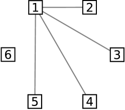
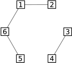
(a)		(b)

Figure 1: Both networks have 4 ties and 4 actors with degree 1. However, in network (b), it is possible to toggle one dyad ($(i,j)=(1,6)$) to create a network with 6 actors with degree 1, something not possible in network (a).

It may be possible to circumvent this problem. If an ERGM is fit to ${\boldsymbol{y}}^{t-1}$’s statistic, as Hanneke et al. (2010) suggest in a slightly different context, it may be possible to approximate the likelihood by integrating over ${\boldsymbol{Y}}^{t-1}$ drawn from the induced ERGM distribution. This may be difficult for reasons similar to those discussed in Section 4.1.

Another disadvantage of CMLE in this context is that it might not make use of all available duration information. The NHSLS survey, for instance, only asked about relationships that ended in the 12 months prior to the survey (and asked for relationship length in months). Even if the problem of conditioning could be circumvented, this means that, at least using the inference of Section 5.1.1, the transition statistic could only be recovered for twelve distinct time points. Any relationships that lasted longer than that — which is most of them — would contribute no additional information. For this reason, we advocate EGMME for these problems.

6 Adjusting the STERGM network evolution process for network size

So far, we have treated the network size and composition as fixed, and focused only on the evolution of network ties. In practice, many dynamic network applications involve actors entering and leaving the network and individual actor attributes changing over time. In this section, we incorporate the adjustments proposed by Krivitsky et al. (2011) into the dynamic models, and explore the properties of the resulting process.

The offset described by Krivitsky et al. (2011) operates as a coefficient on an edge count statistic. As Krivitsky and Handcock (2014) discuss, the edge count statistic in a TERGM transition probability has a dual effect. In particular, an increasingly negative coefficient of the offset term of a growing network would both reduce the incidence and shorten duration. Whether or not this is a desirable property of the model depends on the network process of interest, but in particular, in human sexual relationship networks, there is little reason to believe that duration would change significantly as the population grows or shrinks. Thus, the offset should only affect the incidence of ties. In a separable parametrization, this is easily achieved by only be adding the offset term to the formation phase of the process. In other words,

$$\operatorname{Pr}_{{\boldsymbol{g}}^{+}}({\boldsymbol{Y}}^{+}=y^{+}|{\boldsymbol{Y}}^{t-1}={\boldsymbol{y}}^{t-1};{\boldsymbol{\theta}}^{+})=\\ \frac{\exp\left(\log\left(\frac{1}{n^{(t-1)}}\right)\left\lvert{\boldsymbol{y}}^{+}\right\rvert+{\boldsymbol{\theta}}^{+}\cdot{\boldsymbol{g}}^{+}({\boldsymbol{y}}^{+},{\boldsymbol{y}}^{t-1})\right)1_{{\boldsymbol{y}}^{+}\supseteq{\boldsymbol{y}}^{t-1}}}{c_{{\boldsymbol{g}}^{+}}({\boldsymbol{\theta}}^{+},{\boldsymbol{y}}^{t-1})}$$

for $n^{(t-1)}$ being the number of actors in the network at time $t-1$; and $\operatorname{Pr}_{{\boldsymbol{g}}^{-}}({\boldsymbol{Y}}^{-}=y^{-}|{\boldsymbol{Y}}^{t-1}={\boldsymbol{y}}^{t-1};{\boldsymbol{\theta}}^{-})$ is unchanged.

In particular consider adding a network size offset to the example Section 3.2.3, with edge count formation and edge count dissolution. Adding the offset to formation yields the transition probability:

$$\operatorname{Pr}_{{\boldsymbol{g}}}({\boldsymbol{Y}}^{t}={\boldsymbol{y}}^{t}|{\boldsymbol{Y}}^{t-1}={\boldsymbol{y}}^{t-1};{\boldsymbol{\theta}})=\\ \frac{\exp\left(\left({\boldsymbol{\theta}}^{+}-\log(n)\right)\left\lvert{\boldsymbol{y}}^{t}\cup{\boldsymbol{y}}^{t-1}\right\rvert+{\boldsymbol{\theta}}^{-}\left\lvert{\boldsymbol{y}}^{t}\cap{\boldsymbol{y}}^{t-1}\right\rvert\right)}{c_{{\boldsymbol{g}}}({\boldsymbol{\theta}},{\boldsymbol{y}}^{t-1})},$$

which, substituting into (3), and converting odds to probability gives mean degree, for an undirected network, of

$$(n-1)\operatorname{Pr}_{{\boldsymbol{g}}}({\boldsymbol{Y}}_{i,j}=1;{\boldsymbol{\theta}}) =\frac{(n-1)(1+\exp\left({\boldsymbol{\theta}}^{-}\right))}{1+n\exp\left(-{\boldsymbol{\theta}}^{+}\right)+1+\exp\left({\boldsymbol{\theta}}^{-}\right)},$$

which asymptotically converges to

$$\lim_{n\to\infty}(n-1)\operatorname{Pr}_{{\boldsymbol{g}}}({\boldsymbol{Y}}_{i,j}=1;{\boldsymbol{\theta}}) =\lim_{n\to\infty}\frac{(n-1)(1+\exp\left({\boldsymbol{\theta}}^{-}\right))}{1+n\exp\left(-{\boldsymbol{\theta}}^{+}\right)+1+\exp\left({\boldsymbol{\theta}}^{-}\right)}$$

$$=\exp\left({\boldsymbol{\theta}}^{+}\right)+\exp\left({\boldsymbol{\theta}}^{+}+{\boldsymbol{\theta}}^{-}\right).$$

Thus, the offset term can be used to stabilize and control a dynamic model’s equilibrium mean degree as well.

7 Application to dynamic population simulation based on the National Health and Social Life Survey data

We demonstrate these ideas by taking the National Health and Social Life Survey (NHSLS) data and model fit by Krivitsky et al. (2011), fitting a dynamic version of the model — easily converted from the cross-sectional using implicitly dynamic statistics, and then simulating an evolving and growing population based on the estimated parameters. The EGMME approach is particularly well-suited so problems where the ultimate goal is simulation: in a successful fit, for which $J(\tilde{\boldsymbol{\theta}})=0$ will, by construction, produce a simulation whose expected values of statistics of interest will match those observed exactly.

7.1 Model for network evolution

Our exploratory survival analysis showed that a geometric distribution was an adequate approximation to the duration distribution of a relationship, and that there was little mixing structure in the dissolution hazard. Therefore, we postulate an approximately geometric relationship duration distribution, and set ${\boldsymbol{g}}^{-}({\boldsymbol{y}}^{-},{\boldsymbol{y}}^{t-1})=\left\lvert{\boldsymbol{y}}^{-}\right\rvert.$

This means that we attribute all the structure in the network to differences in incidence of relations. Per Krivitsky and Handcock (2014), this makes some intuitive sense: once a relationship is formed, its persistence is likely affected by fewer factors than its formation. Thus, we “convert” the NHSLS model of Krivitsky et al. (2011) to a dynamic one by only using Inherited statistics and setting the formation statistic ${\boldsymbol{g}}^{+}({\boldsymbol{y}}^{+})$ to the same statistic as that in that article (though evaluated on ${\boldsymbol{y}}^{+}$ rather than on ${\boldsymbol{y}}$). The terms used are listed in Table 1 and described in more detail by Krivitsky et al. (2011). We also add a network size offset of Section 6.

7.2 Inference

We now describe the procedure for fitting this model to the available data.

7.2.1 Target statistic

Because our goal is simulation, and for simplicity, we set

$${\boldsymbol{t}}({\boldsymbol{y}})=\left({\boldsymbol{g}}^{+}({\boldsymbol{y}}),\frac{1}{\left\lvert{\boldsymbol{y}}\right\rvert}\sum_{(i,j)\in{\boldsymbol{y}}}\operatorname{age}({\boldsymbol{y}}_{i,j})\right),$$

the formation generative statistic evaluated on the cross-sectional network (simulated or inferred) and the average age of an extant tie in this network. This also serves to simplify fitting of this model, because one can fairly safely assume that ${\boldsymbol{G}}({\boldsymbol{\theta}})$ has a positive diagonal: $\partial{\boldsymbol{\mu}}({\boldsymbol{\theta}}_{k})/\partial{\boldsymbol{\theta}}_{k}>0$.

For this demonstration, we resample the egos in the network to resample size 1000.

7.2.2 Time step size

How much time is represented by a single discrete time step is a trade-off between granularity and computational cost: shorter time steps have a higher cost to simulate, while longer time steps make the separability assumption that formation and dissolution are conditionally independent within a time step less plausible. (Krivitsky and Handcock, 2014) Driven in part by the format of the data, where all duration measurements are integral counts of months, we set

$$1\text{ time step}=1\text{ month}=\frac{1}{12}\text{ year}.$$

7.2.3 Time-varying exogenous covariates

A network series simulated under ${\boldsymbol{\theta}}$ of interest converges to equilibrium, and statistics of that chain can be used as input to the search for EGMME. However, the model used includes effects of actors’ ages and age differences on relationship incidence, and actors age over time. When fitting model parameters, we ignore this: even as the network evolution process runs forward, all actors’ ages stay the same. Nor are actors added or removed from the network. This is likely to produce biased estimates, such that the simulation stage, which does incorporate these vital dynamics, will not reproduce the statistics of interest exactly, particularly the age-related statistics.

7.3 Simulation

We simulate the evolution of a network of sexual partnerships based on the network process described above, over 500 simulation years (6,000 1-month time steps), incorporating a model with vital dynamics: aging (with actors aging out of the population at 60, maintaining a closed network of 18–59), actors randomly removed from the population, and actors randomly “reproducing”, to test the network size adjustment.

7.3.1 Population process model

We use a starting network constructed out of the resampled “egos”, with simulated annealing used to find a particular configuration of ties that has cross-sectional target statistic similar to that inferred. In the network (tie) evolution model, we assume that tie formation and dissolution do not affect each other within a time step, and our incorporation of vital dynamics is done similarly: within each time step the network evolution process takes place, then population evolution process (not affected by network evolution process) takes place. Thus, within a time step, the vital dynamics changes do not affect the network process, and the network process does not affect the vital dynamics changes.

The following procedure is iterated every time step (month):

1. The network evolution model, adjusted for network size, is run one time step forward, forming and dissolving network ties.

2. For each actor, with probability 0.0023, an identical actor, but aged 18 and with sex selected at random is added to the population.

3. For each actor, with probability 0.00042, the actor is removed from the population.

4. Actors’ ages are incremented by 1 month.

5. For each actor, if the actor’s age equals or exceeds 60, the actor is also removed from the population.

6. All ties incident on removed actors are dissolved.

7. The state of the population is recorded.

The specific values for “birth rate”, “death rate” were selected to give a modest but substantial population growth over the length of the simulation.

7.4 Implementation

Some of the difficulties associated with fitting these models and the algorithm we use are discussed in Appendix A. As a simple shortcut, we use (4) to estimate

$$\tilde{{\boldsymbol{\theta}}}=-\operatorname{logit}\left(\left(\frac{1}{\left\lvert{\boldsymbol{y}}\right\rvert}\sum_{(i,j)\in{\boldsymbol{y}}}\operatorname{age}({\boldsymbol{y}}_{i,j})\right)^{-1}\right).$$

Software package ergm (Hunter et al., 2008b; Handcock et al., 2012) in the statnet (Handcock et al., 2008) suite of libraries for social network analysis in R (R Development Core Team, 2009) was used to fit and simulate from these models, with the package networkDynamic (Leslie-Cook et al., 2012) used to store and inspect the simulation results.

7.5 Results

7.5.1 Model fit

The inferred equilibrium target statistic and EGMME parameters are given in Table 1. To test the fit, we simulated a network series from the model over a static population: same values for ${\boldsymbol{\theta}}^{+}$ and ${\boldsymbol{\theta}}^{-}$ were used and the same initial network, but no actors were added or removed, and actor ages were held fixed. The simulated values (shown in Figure 2) are essentially the same as those observed, suggesting that the correct fit was found. For interpretability, we normalize network statistics we report as follows:

1. if a statistic pertains directly to a particular subset of actors, (e.g. a particular sex or race category), it is normalized by the total number of actors in that subset at the time;

2. otherwise, the statistic is normalized by the overall network size at the time.

Thus, for example, the statistic reported for the actor activity by sex for males is the number of ties incident on male actors (with male-male ties counting twice) divided by the number of male actors: that is, the mean degree of a male in the network. Similarly, the statistic for the monogamy for females (number of female actors with degree 1) is reported as the proportion of the total number of female actors in the network. On the other hand, age effects do not pertain to any particular group, and are thus normalized by the whole network’s size.

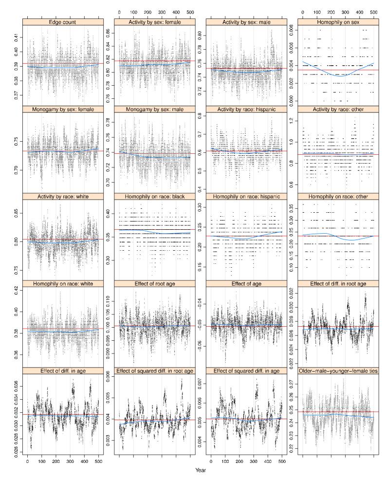
Figure 2: NHSLS dynamic simulation network statistics over time, in a static population. All values are normalized per Section 7.5.1. Red lines are the “target” values for their respective statistics.

Table 1: Parameter estimates and simulation results
All network statistics (${\boldsymbol{t}}$) are per capita in the group they describe (per Section 7.5.1); times are in years.

	Inference		Simulation
	${\boldsymbol{t}}({\boldsymbol{y}})$	$\tilde{\boldsymbol{\theta}}$	${\boldsymbol{t}}({\boldsymbol{Y}}^{100})$	${\boldsymbol{t}}({\boldsymbol{Y}}^{300})$	${\boldsymbol{t}}({\boldsymbol{Y}}^{500})$
Network size	$1000$	$1000$	$1469$	$2111$	$3227$
Formation
Offset		$-6.908$
Actor activity by sex
Female	$0.819$	$-4.563$	$0.713$	$0.740$	$0.715$
Male	$0.756$	$-5.520$	$0.717$	$0.713$	$0.701$
Same-sex partnership	$0.004$	$-4.318$	$0.005$	$0.004$	$0.004$
Monogamy by sex
Female	$0.735$	$2.007$	$0.637$	$0.694$	$0.658$
Male	$0.740$	$2.793$	$0.717$	$0.701$	$0.692$
Actor activity by race
Black	(base)	(base)
Hispanic	$0.614$	$0.770$	$0.504$	$0.478$	$0.414$
Other	$0.900$	$2.605$	$0.820$	$0.898$	$0.905$
White	$0.806$	$1.175$	$0.726$	$0.735$	$0.710$
Race homophily by race
Black	$0.366$	$6.334$	$0.347$	$0.316$	$0.341$
Hispanic	$0.228$	$3.226$	$0.160$	$0.147$	$0.133$
Other	$0.233$	$2.724$	$0.220$	$0.320$	$0.319$
White	$0.384$	$2.017$	$0.344$	$0.349$	$0.337$
Age effects
$\sqrt{\text{age}}$ effect	$0.101$	$3.725$	$0.127$	$0.136$	$0.135$
age effect	$-0.051$	$-2.735$	$0.002$	$0.010$	$0.011$
Age difference effects
Difference in $\sqrt{\text{age}}$	$0.027$	$-5.801$	$0.019$	$0.018$	$0.018$
Difference in age	$0.032$	$-9.012$	$0.025$	$0.024$	$0.023$
Squared difference in $\sqrt{\text{age}}$	$0.004$	$5.234$	$0.002$	$0.002$	$0.002$
Squared difference in age	$0.005$	$2.264$	$0.004$	$0.003$	$0.003$
Older-male-younger-female	$0.249$	$1.116$	$0.176$	$0.178$	$0.158$
Dissolution
Mean duration (years)	$10.307$	$4.810$	$7.160$ raw, $10.181$ adjusted

7.5.2 Evolution of network structure

Over the course of the simulation with evolving size and composition, the population grew from 1,000 actors to 3,227 actors (shown in Figure 3(a)), with a total of 28,652 individuals in the population during the period. Because the population is fairly small and the population growth is exponential, there were substantial changes in population composition (shown in Figure 3(b)).

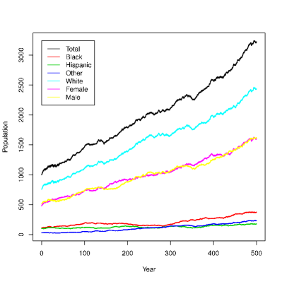
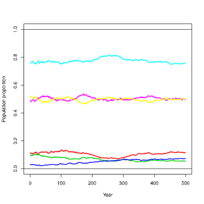
(a) subpopulation sizes	(b) subpopulation proportions

Figure 3: NHSLS dynamic simulation population (network size) and subpopulation sizes and proportions over time.

We give snapshots of cross-sectional network statistics at $t=100$, $t=300$, and $t=500$ years in table Table 1. Plots of trends over time are given in Figure 4.

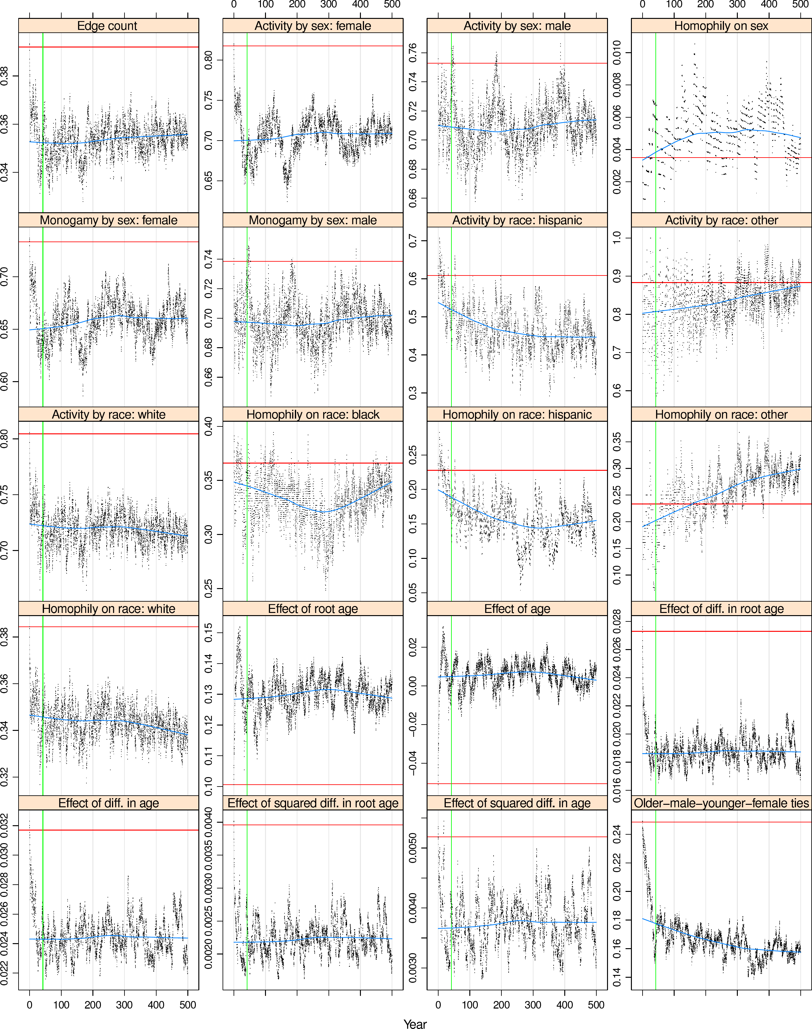
Figure 4: NHSLS dynamic simulation network statistics over time, in a growing population. All values are normalized per Section 7.5.1. Red lines are the “target” values for their respective statistics; green line is the time point at which no actors from the original population remain.

The simulation of the evolving population removes individuals and their ties from the network, and adds only individuals with no ties, something not taken into account by the algorithm used to fit the parameters, so, after a short “burn-in” period, the mean degree of the network is uniformly lower than that targeted. Beyond that, the mean degree (and other such statistics) do not appear to be sensitive to network size, but do appear to be sensitive to the population composition: the trends in racial-category-specific mean degrees (Figure 4, the “homophily on race” and “activity by race” panels) closely follow those in the population (Figure 3(b)). This is what the model of Krivitsky et al. (2011) predicts, assuming the “preferences” as modeled remain unchanged: the more rare a given individual’s preferred partners are in the population, the lower the expected mean degree for that individual.

7.5.3 Duration distribution

The approach of Section 7.4 gives a target mean duration of 10.31 years, but because about 28% of ties in the history of the simulated network had been censored due to the actor being removed from the population of interest and 2% of ties had been censored due to the simulation ending, the average duration of a tie that is simulated is 7.16 years. Using a Kaplan-Meier estimator (Therneau, 2009) to estimate the survival function $1-F(x)$, and estimating the mean of duration by integrating it (Klein and Moeschberger, 2003, 117–118) gives an adjusted mean duration of 10.18 years, slightly smaller than the target, likely due to no simulated tie having duration greater than $60-18=42$ years.

All this suggests that this model is at the very least viable for simulating networks in populations with changing size, based on fairly limited data.

8 Discussion

We began with the model of Krivitsky and Handcock (2014), described its long-run properties, especially in the simpler and more tractable special cases; and discussed approaches — both feasible and not — to fitting these network evolution processes to sociometric data that are not, at first glance, amenable to dynamic network modeling. We have also described how the network size adjustment of Krivitsky et al. (2011) may be incorporated into this model and demonstrated its efficacy with an application to the NHSLS survey.

Many simplifying assumptions were made in the simulation, aspects left unanalyzed, and questions unanswered about the properties of the models discussed. We describe some of them here.

The EGMME approach depends on a very strong assumption, that the social process being modeled does not significantly change over time in ways that the model does not account for, so the network data observed can be plausibly modeled a draw from an equilibrium distribution. It is not clear whether this assumption can be tested, especially if only egocentrically sampled data are available, beyond the generic goodness-of-fit measures like those of Hunter et al. (2008a). Conditional approaches do not suffer from this, but, as we showed in Section 5.1.2, require data not often available, and methods to circumvent this problem also require fairly strong assumptions, though those assumptions are arguably weaker than those needed for full equilibrium inference.

Although we have discussed the effects of dyadic dependence in the dissolution phase of the process, we have not discussed nor demonstrated how its parameters might be fit. In particular, in a sexual partnership network, it is very plausible that monogamous ties are much more stable than those that are concurrent. This effect can be modeled in a STERGM with a generative statistic

$${\boldsymbol{g}}^{-}_{k}({\boldsymbol{y}}^{-},{\boldsymbol{y}}^{t-1})=\sum_{i\in N}1_{\left\lvert{\boldsymbol{y}}^{-}_{i}\right\rvert=1}.$$

But, if there is expected to be monogamy bias in formation as well, if the only target statistic with information about degree is

$${\boldsymbol{t}}_{k}({\boldsymbol{y}})=\sum_{i\in N}1_{\left\lvert{\boldsymbol{y}}_{i}\right\rvert=1},$$

the monogamy biases in formation and dissolution may not be identified. A duration-sensitive target statistic like

$${\boldsymbol{t}}_{k^{\prime}}({\boldsymbol{y}},\dotsc)=\frac{1}{n}\sum_{i\in N}1_{\left\lvert{\boldsymbol{y}}_{i}\right\rvert=1}\sum_{j\in{\boldsymbol{y}}_{i}}\operatorname{age}({\boldsymbol{y}}_{i,j}),$$

the average duration of all monogamous ties, used alongside ${\boldsymbol{t}}_{k}$, may be able to identify the incidence effects from the duration effects, and can be inferred from short-term relationship history: all that is needed is to know whether a relationship was monogamous at the time of the survey and how long the relationship had lasted.

While the simulation incorporated vital dynamics to demonstrate invariance to network size, the procedure used to fit the parameters did not take into account vital dynamics in any way. Taking vital dynamics into account when learning $\tilde{{\boldsymbol{\theta}}}$ is a subject of ongoing research. One way to do so may be to simulate the effects of aging and of actors aging out of population of interest (18–59 in the example above) or otherwise being removed, then “resetting” the age of each removed actor to the age of a neophyte (18 in this case) breaking all of the actor’s ties, and reinserting that actor into the population. Such a process would have a stationary distribution, especially if the removal process were at least somewhat stochastic to render the combined process aperiodic, and it thus could still be used for simulated EGMME, but its estimates for the expected values of the target statistic under a particular parameter configuration would at least partly reflect the vital dynamics.

The GMME approach to network inference can be extended to other “inconvenient” data: while the targeted statistics we have used to date have been network statistics, they do not have to be: for example, infection tree data may contain information about the underlying network process: rather than finding that network process which produces networks having statistics similar to those that have been observed, it may be possible to find that network process which produces networks, infection processes on which produce infection trees with similar features to those observed, as an alternative to the method of Groendyke et al. (2011).

9 Acknowlegements

This work was supported by NIH awards R21 HD063000-01, P30 AI27757, and 1R01 HD068395-01, NSF award MMS-0851555 and HSD07-021607, ONR award N00014-08-1-1015, NICHD Grant 7R29HD034957, NIDA Grant 7R01DA012831, the University of Washington Networks Project, and Portuguese Foundation for Science and Technology Ciência 2009 Program. The author would also like to thank David Hunter and Mark Handcock, as well as the members of the University of Washington Network Modeling Group, especially Martina Morris and Steven Goodreau, for their helpful input and comments on the draft.

Appendix A Finding a Generalized Method of Moments Estimator

Finding a GMME in our setting presents several unusual challenges. The objective function (8) can only be estimated by simulation, necessitating some sort of stochastic approximation. However, many network processes of interest, such as sexual partnership networks, evolve slowly, with relationships lasting months or years, even decades. On the other hand, the plausibility of the separability assumption improves as the length of each discrete time step increases (Krivitsky and Handcock, 2014). Thus, successive networks drawn from the model are likely to be very similar — highly autocorrelated. This, in turn, means that a sufficiently precise estimate of $J({\boldsymbol{\theta}})$ requires simulating a very long series of such networks.

Finding the direction of the stochastic search presents a further challenge. In gradient-based methods,

$$\nabla J({\boldsymbol{\theta}})=\left({\boldsymbol{\mu}}({\boldsymbol{\theta}})-{\boldsymbol{t}}({\boldsymbol{y}}^{1},\dots,{\boldsymbol{y}}^{T})\right)^{\top}{\boldsymbol{V}}({\boldsymbol{\theta}})^{-1}{\boldsymbol{G}}({\boldsymbol{\theta}}).$$

Some specific combinations of ${\boldsymbol{t}}$ and ${\boldsymbol{g}}$ suggest some simple relationship for ${\boldsymbol{G}}$. For example, if ${\boldsymbol{t}}_{k}({\boldsymbol{y}}^{t})\equiv\left\lvert{\boldsymbol{y}}^{t}\right\rvert$ and ${\boldsymbol{g}}_{l}({\boldsymbol{y}}^{t},{\boldsymbol{y}}^{t-1})\equiv\left\lvert{\boldsymbol{y}}^{t}\cup{\boldsymbol{y}}^{t-1}\right\rvert$ (i.e., edge count formation), it is likely that the ${\boldsymbol{G}}_{k,l}({\boldsymbol{\theta}})>0$. However, for less strongly related statistics, the gradient would need to be estimated.

Nor are the signs of elements of the ${\boldsymbol{G}}({\boldsymbol{\theta}})$ guaranteed to remain the same throughout the parameter space. For example, if ${\boldsymbol{t}}_{k}({\boldsymbol{y}}^{t})\equiv\sum_{i=1}^{n}1_{\left\lvert{\boldsymbol{y}}^{t}_{i}=1\right\rvert}$ — the number of actors with degree 1 — and ${\boldsymbol{g}}_{l}$ is as before, then the gradient is likely to be positive when ${\boldsymbol{\theta}}_{l}$ is low, and most actors are isolates, since an increase in ${\boldsymbol{\theta}}_{l}$ increases the number who have one tie; but as ${\boldsymbol{\theta}}_{l}$ increases to the point where some actors begin to acquire their second tie, its effect on the number of actors with one tie reverses, to the point where increasing ${\boldsymbol{\theta}}_{l}$ makes it increasingly less likely that an actor will have fewer than two ties. Thus, the gradient matrix must be estimated and reestimated continually throughout the search.

Selection of starting values for the optimization presents yet another challenge. As with ordinary ERGMs, a poor choice of starting parameter configuration may induce extreme network distributions, in the sense that ${\boldsymbol{\mu}}({\boldsymbol{\theta}}_{0})$ is close to the edge of the convex hull of possible network statistics, which, in the discrete space of networks, makes it almost impossible to estimate ${\boldsymbol{\mu}}_{k}({\boldsymbol{\theta}}_{0})$, because almost all equilibrium draws ${\boldsymbol{t}}_{k}({\boldsymbol{Y}}^{t})$ under ${\boldsymbol{\theta}}_{0}$ equal to $\min_{{\boldsymbol{y}}\in\mathcal{Y}}{\boldsymbol{t}}_{k}({\boldsymbol{y}})$ or $\max_{{\boldsymbol{y}}\in\mathcal{Y}}{\boldsymbol{t}}_{k}({\boldsymbol{y}})$. Unlike ordinary ERGMs, where the Maximum Pseudolikelihood Estimator (MPLE) provides a plausible ${\boldsymbol{\theta}}_{0}$, we are aware of no such methods. Thus, the optimization method must be relatively robust to poor starting values. In particular, if the initial configuration has some expectations be near their minimal or maximal values but not others, the algorithm should not necessarily fail: perhaps finding a parameter configuration where ${\boldsymbol{\mu}}_{k}({\boldsymbol{\theta}})$ is close to ${\boldsymbol{t}}_{k}({\boldsymbol{y}}^{1},\dots,{\boldsymbol{y}}^{T})$ for some $k$ will shift others to a more convenient region. An example of this is ${\boldsymbol{t}}({\boldsymbol{y}}^{t})\equiv(\left\lvert{\boldsymbol{y}}^{t}\right\rvert,\sum_{i=1}^{n}1_{\left\lvert{\boldsymbol{y}}^{t}_{i}=1\right\rvert})^{\top}$: that if that an initial parameter configuration inducing overly dense networks can cause ${\boldsymbol{\mu}}_{2}({\boldsymbol{\theta}}_{0})\approx 0$, but if further optimization using ${\boldsymbol{\mu}}_{1}$ brings the network density down to where more actors have one tie, the estimation could begin to incorporate the second statistic.

We have tried a number of approaches, including Kiefer-Wolfowitz (Kiefer and Wolfowitz, 1952) and Simultaneous Perturbation Stochastic Approximation (SPSA) (Spall, 1998), but we have ultimately found that simple gradient descent updating, with

$${\boldsymbol{\theta}}^{t}={\boldsymbol{\theta}}^{t-1}-\gamma_{t}\left(\hat{{\boldsymbol{\mu}}}({\boldsymbol{\theta}}^{t-1})-{\boldsymbol{t}}({\boldsymbol{y}}^{1},\dots,{\boldsymbol{y}}^{T})\right)^{\top}\hat{{\boldsymbol{V}}}({\boldsymbol{\theta}}^{t-1})^{-1}\hat{{\boldsymbol{G}}}({\boldsymbol{\theta}}^{t-1})$$

works adequately, with $\gamma_{t}$ being a declining sequence, ${\boldsymbol{\mu}}({\boldsymbol{\theta}}^{t})$ estimated by simulation, ${\boldsymbol{G}}({\boldsymbol{\theta}}^{t})$ being estimated by regressing recent values of ${\boldsymbol{t}}({\boldsymbol{Y}}^{t})$ on ${\boldsymbol{\theta}}^{t}$ (and an intercept). The covariance of the residuals from this regression is then used to estimate ${\boldsymbol{V}}({\boldsymbol{\theta}}^{t})$. The resulting process produces a Continuous-Updating Estimator. (Hansen et al., 1996)

References

- Butts (2008) Carter T. Butts. A relational event framework for social action. Sociological Methodology, 38(1):155–200, 2008. doi: 10.1111/j.1467-9531.2008.00203.x.
- Casella and Berger (2002) George Casella and Roger L. Berger. Statistical inference. Duxbury Advanced Series. Duxbury Pacific Grove, CA, 2nd edition, 2002.
- Doreian and Stokman (1997) Patrick Doreian and Franz N. Stokman, editors. Evolution of social networks. Routledge, 1997.
- Frank (1991) Ove Frank. Statistical analysis of change in networks. Statistica Neerlandica, 45(3):283–293, 1991. doi: 10.1111/j.1467-9574.1991.tb01310.x.
- Groendyke et al. (2011) Chris Groendyke, David Welch, and David R Hunter. Bayesian inference for contact networks given epidemic data. Scandinavian Journal of Statistics, 38(3):600–616, 2011. doi: 10.1111/j.1467-9469.2010.00721.x.
- Handcock et al. (2008) Mark S. Handcock, David R. Hunter, Carter T. Butts, Steven M. Goodreau, and Martina Morris. statnet: Software tools for the representation, visualization, analysis and simulation of network data. Journal of Statistical Software, 24(1):1–11, May 2008. doi: 10.18637/jss.v024.i01.
- Handcock et al. (2012) Mark S. Handcock, David R. Hunter, Carter T. Butts, Steven M. Goodreau, Pavel N. Krivitsky, and Martina Morris. ergm: A Package to Fit, Simulate and Diagnose Exponential-Family Models for Networks. The Statnet Project, Seattle, WA, version 3.0-1 edition, March 2012. URL http://CRAN.R-project.org/package=ergm. Version 3.0-1. Project home page at http://www.statnet.org.
- Hanneke et al. (2010) Steve Hanneke, Wenjie Fu, and Eric P. Xing. Discrete temporal models of social networks. Electronic Journal of Statistics, 4:585–605, 2010. doi: 10.1214/09-EJS548.
- Hansen et al. (1996) Lars Peter Hansen, John Heaton, and Amir Yaron. Finite-sample properties of some alternative GMM estimators. Journal of Business & Economic Statistics, 14(3):262–280, July 1996. doi: 10.2307/1392442.
- Harris et al. (2003) Kathleen M. Harris, F. Florey, Joyce Tabor, Peter S. Bearman, J. Jones, and J. Richard Udry. The national longitudinal study of adolescent health: Research design. Technical report, University of North Carolina, 2003. URL http://www.cpc.unc.edu/projects/addhealth/design/.
- Helleringer and Kohler (2007) Stéphanie Helleringer and Hans-Peter Kohler. Sexual network structure and the spread of HIV in Africa: evidence from Likoma Island, Malawi. AIDS, 21(17):2323–2332, 2007. doi: 10.1097/qad.0b013e328285df98.